


1. Introduction
Over the past 20 or 30 years, our understanding of the scaling and structure of wall-bounded turbulent flows has advanced greatly. Direct numerical simulations (DNS) and large-eddy simulation have made extraordinary contributions to our understanding as computational resources have exploded and numerical methods continue to evolve, while experiments have benefited from advances in instrumentation that have provided unprecedented accuracy and detail. We have also seen an intimate convergence of experiment and computation that has accelerated progress even further. In particular, canonical wall-bounded flows such as flat plate, zero pressure gradient boundary layers and fully developed pipe and channel flows are now known to display many similarities in the scaling of their mean velocity and turbulence distributions, and this convergence is especially clear at high Reynolds number. Here, we focus on some of the contributions made by experiment to this progress in understanding.
Measurements in turbulence rely on three basic tools: hot-wire anemometry; laser Doppler velocimetry (LDV); and particle image velocimetry (PIV). Pitot probes are also often used to measure the local dynamic pressure, and when combined with a separate measurement of the static pressure (often achieved using a static pressure tap in the wall) will yield the local mean velocity. Hot-wire anemometry uses a heated wire sensor that is inserted into the flow field, and by monitoring the voltage supplied to the sensor to keep either its resistance or its current constant the instrument provides (using a suitable calibration technique) a continuous time history of the flow velocity at a point. It is possible to measure different components of the velocity fluctuations by using multiple sensors, but in its most common form (the normal wire) it measures only the streamwise component. This method has a long history, and there is a wealth of literature available on its strengths and limitations (see, for example, Comte-Bellot Reference Comte-Bellot1976; Freymuth Reference Freymuth1978; Perry Reference Perry1982; Smoliakov & Tkachenko Reference Smoliakov and Tkachenko1983; Lomas Reference Lomas1986; Fingerson Reference Fingerson1994; Bruun Reference Bruun1995).
In LDV and PIV, the flow is seeded with small particles and their motion is tracked using optical methods. Both LDV and PIV are considered to be non-intrusive methods, in that there is no physical sensor present in the flow. In LDV, the measurement volume is defined by the crossing of a pair of focused laser beams, and a single velocity component is found by recording the Doppler shift in the scattered light as particles pass through the measurement volume (see, for instance, Adrian & Goldstein Reference Adrian and Goldstein1971; George & Lumley Reference George and Lumley1973; Durst, Melling & Whitelaw Reference Durst, Melling and Whitelaw1976; Tropea Reference Tropea1995). It is possible to measure more than one component of velocity by collocating the measurement volumes created by multiple pairs of laser beams. In PIV the seeding particles are illuminated by a light emitting diode or laser sheet, and by using a camera to record two successive images of the particles the velocity at any point in the imaged field can be found by correlation or particle tracking techniques. The method yields two components of the velocity fluctuations at the same time, and by using two cameras it can also give the third component in the plane of the laser sheet (this is called stereo PIV or sPIV). Tomographic and holographic techniques can extend the data to a volume, although PIV is used most commonly in its planar or stereo mode. Its application has blossomed since its introduction in the early 1980s, and it has had a major influence on our ability to measure and visualize turbulence (Adrian Reference Adrian1984; Adrian & Westerweel Reference Adrian and Westerweel2011; Westerweel, Elsinga & Adrian Reference Westerweel, Elsinga and Adrian2013).
A comprehensive review of these techniques is well beyond the scope of the present contribution. Instead, I consider how recent advances have helped to answer some key questions on how turbulent wall-bounded flow develops with Reynolds number. This quest naturally prioritizes studies at high Reynolds number so that scaling trends can be identified, and there is always an underlying need for accuracy since we know from experience that such variations are subtle. My survey is rather selective, in that I am primarily concerned with statistical measures of turbulence, and the particular topics are framed in terms of the expectations derived from theory or scaling arguments. We start with mean flow considerations before tackling the turbulent stress behaviour.
2. Mean flow scaling
One of the landmark results in wall-bounded turbulence is the presence of a logarithmic region in the mean velocity (Prandtl Reference Prandtl1925; von Kármán Reference von Kármán1930). It is often cast as a region of overlap (Millikan Reference Millikan1938), where the inner-scaled wall region overlaps with the outer-scaled outer region. In general we write, for isothermal, incompressible, wall-bounded flow
 \begin{equation} [U_i,\overline{u_i u_j}] = f(y, u_\tau, \nu, \delta),\end{equation}
where  $U_i$ and
  $u_i$ are the mean and fluctuating velocities in the
  $i$th direction, and
  $y$ is the distance from the wall. The overbar denotes time averaging, and
  $\delta$ is, as appropriate, the boundary layer thickness, the pipe radius, or the channel half-height. The friction velocity
  $u_\tau =\sqrt {\tau _w/\rho }$, where
  $\tau _w$ is the wall stress and
  $\rho$ and
  $\nu$ are the fluid density and kinematic viscosity, respectively. Equation (2.1) assumes that there is only a single velocity scale for the entire layer, given by
  $u_\tau$. A separate outer velocity scale,
  $u_0$, was proposed by Zagarola & Smits (Reference Zagarola and Smits1998a), where
  $u_0=U_\infty \delta ^*/\delta$ (
 $U_\infty$ is the free stream or centreline velocity and
  $\delta ^*$ is the displacement thickness). For pipe flows and boundary layers, the collapse of the mean velocity was noticeably improved when using
  $u_0$ instead of
  $u_\tau$ for
  $y/\delta > 0.07$ and for
  $650 < Re_\tau < 18 \times 10^3$ (Zagarola & Smits Reference Zagarola and Smits1998a,Reference Zagarola and Smitsb). At higher Reynolds numbers, however,
  $u_0$ becomes proportional to
  $u_\tau$ so that it appears that
  $u_\tau$ can be used to scale both the inner and outer layers if the Reynolds number is sufficiently high. By dimensional analysis, we can then write the functional dependence given by (2.1) in two ways,
 \begin{align} [U_i^+,\overline{u_i u_j}^+] & = f(y^+, Re_\tau) \end{align}
 \begin{align} \hbox{or} \quad [U_i^+,\overline{u_i u_j}^+] & = f(y/\delta, Re_\tau), \end{align}
where the friction Reynolds number is  $Re_\tau =\delta u_\tau /\nu$ and the superscript ‘
 $+$’ denotes non-dimensionalization by the velocity scale
  $u_\tau$ and the ‘inner’ length scale
  $\nu /u_\tau$ (for example,
  $y^+=y u_\tau /\nu$). Near the wall the inner length scale is of the same order as the Kolmogorov length scale
  $\eta$, and so it is characteristic of the smallest scales in the flow, while the outer length scale
  $\delta$ is a measure of the largest scales. The friction Reynolds number therefore measures the separation between the largest and smallest scales. The form given by (2.2) is called inner scaling, and that given by (2.3) is called outer scaling. For convenience, we will use
  ${U}$ for the mean and
  $u$ for the fluctuating velocity component in the streamwise direction, and so the corresponding non-dimensional stress is given by
  $\overline {u^2}^+ = \overline {u^2}/u_\tau ^2$.
The central role of the Reynolds number is clear from (2.2) and (2.3): as the Reynolds number goes to very large values, these relationships imply that the inner part of the flow becomes a function of  $y^+$ only and the outer flow becomes a function of
  $y/\delta$ only. At sufficiently high Reynolds number, Millikan (Reference Millikan1938) proposed that there may be a region that spans
  $y^+ \gg 1$ and
  $y/\delta \ll 1$ where (2.2) and (2.3) overlap. By assuming that Reynolds number effects are negligible and by matching the mean velocity gradients for the inner and outer regions in this ‘overlap’ region, we obtain
 \begin{equation} \frac{\partial U}{\partial y} = \frac{u_\tau}{\kappa y} = \frac{\sqrt{\tau_w/\rho}}{\kappa y},\end{equation}
where  $\kappa$ is the von Kármán constant. For this overlap region, the length scale is simply the distance from the wall. By integration, we obtain the inner and outer forms of the log law for the mean velocity:
 $$\begin{gather} U^+ = \frac{1}{\kappa} \ln{y^+} +B, \end{gather}$$
 $$\begin{gather}U_\infty^+{-}U^+ = -\frac{1}{\kappa} \ln{y/\delta} +B_1. \end{gather}$$
Note that the additive constant  $B$ depends on the lower limit of integration in
  $y$ and so it may depend on Reynolds number (see, for example, Duncan, Thom & Young Reference Duncan, Thom and Young1970; Schlichting Reference Schlichting1979; Zagarola & Smits Reference Zagarola and Smits1998a). For all reasonable Reynolds numbers, however, it appears that
  $B$ can be assumed to be constant.
The log law for the mean velocity was derived as early as 1925 by Prandtl using his mixing length theory combined with the assumption of constant stress (Prandtl Reference Prandtl1925). A few years later, Nikuradse's measurements in a pipe provided extensive data to support the presence of this log law, with constants  $\kappa =0.4$ and
  $B=5.5$ (Nikuradse Reference Nikuradse1932). Can new experiments add anything to this almost totemic result? As it turns out, they can contribute much.
3. Mean flow measurements
There are three basic requirements for any serious investigation of the log law for the mean velocity. First, the friction velocity must be known accurately because it is a crucial scaling parameter. Second, the Reynolds number must be sufficiently high so that there is adequate separation between the inner and outer scales. Third, precise measurements of the velocity are necessary to deduce the slope of the line, that is, von Kármán's constant  $\kappa$, since the errors that arise from differentiating discrete data are well known. In addition, any error in evaluating
  $\kappa$ will also affect the deduced value of the additive constant
  $B$.
$B$.
To satisfy the first criterion, the preferred flow configuration is either fully developed pipe or channel flow because the friction velocity can be found with high precision by simply measuring the pressure drop (for pipes  $u_\tau ^2 = -(D/4)\, {\rm d} p/{{\rm d}\kern0.06em x}$, where
  ${\rm d} p/{{\rm d}\kern0.06em x}$ is the pressure gradient). Direct and accurate measurements of the friction velocity in boundary layers is much more difficult, although oil drop methods have made considerable progress (Naughton & Sheplak Reference Naughton and Sheplak2002; Segalini, Rüedi & Monkewitz Reference Segalini, Rüedi and Monkewitz2015; Lee et al. Reference Lee, Nonomura, Asai and Naughton2019).
To satisfy the criterion for high Reynolds number, a number of new, purpose-built facilities are now available, as discussed by Smits (Reference Smits2020). The older facilities capable of reaching high Reynolds numbers were largely designed for aeronautical or atmospheric flow investigations, and usually did not have the required flow quality for fundamental turbulent boundary layer studies. The newer facilities include the Princeton SuperPipe (Zagarola & Smits (Reference Zagarola and Smits1998a); figure 1a), the Stanford high-pressure tunnel (De Graaff & Eaton Reference De Graaff and Eaton2000), the Princeton High Reynolds number Testing Facility (HRTF) (Jiménez, Hultmark & Smits Reference Jiménez, Hultmark and Smits2010), the high Reynolds number boundary layer wind tunnels at the University of New Hampshire (Vincenti et al. Reference Vincenti, Klewicki, Morrill-Winter, White and Wosnik2013) and the University of Melbourne (Marusic et al. (Reference Marusic, Chauhan, Kulandaivelu and Hutchins2015); figure 1b), the large-scale pipe flow facility at the Center for International Cooperation in Long Pipe Experiments (CICLoPE) (Örlü et al. Reference Örlü, Fiorini, Segalini, Bellani, Talamelli and Alfredsson2017; Willert et al. Reference Willert, Soria, Stanislas, Klinner, Amili, Eisfelder, Cuvier, Bellani, Fiorini and Talamelli2017) and the pipe flow experiments at the National Metrology Institute of Japan (NMIJ) (Furuichi, Terao & Tsuji Reference Furuichi, Terao and Tsuji2017; Furuichi et al. Reference Furuichi, Terao, Wada and Tsuji2018). The first three use high-pressure air as the working fluid to achieve high Reynolds number, whereas the others use air at atmospheric pressure, except for the NMIJ pipes which use water. The SuperPipe, CICLoPE and NMIJ were built to study pipe flows, while the others were focused on boundary layers. There are no channel flow facilities with sufficiently high Reynolds number to provide definitive evidence for Reynolds number trends. There are good reasons for this, as discussed in part by Vinuesa et al. (Reference Vinuesa, Noorani, Lozano-Durán, El Khoury, Schlatter, Fischer and Nagib2014), but it is nevertheless somewhat unfortunate given that DNS has mostly focused on two-dimensional channel flows.

Figure 1. High Reynolds number test facilities. (a) Princeton SuperPipe covering the range  $1000 \le Re_\tau =500\,000$ (Zagarola & Smits Reference Zagarola and Smits1998a). (b) Melbourne University High Reynolds Number Boundary Layer Wind Tunnel covering the range
  $2000 \le Re_\tau \le 30\,000$ (Marusic et al. Reference Marusic, Chauhan, Kulandaivelu and Hutchins2015).
To help satisfy the third criterion for precise measurements of velocity, Bailey et al. (Reference Bailey2013) examined ways for making Pitot tubes more accurate, while also evaluating the performance of hot-wire probes for mean velocity measurements. They found that with careful attention to all the sources of error the two techniques could give mean velocity data to within 1 % of each other over most of the velocity profile. The Pitot probe is often preferred over the hot wire because of its inherent simplicity and straightforward implementation. However, it is necessary to make a number of corrections to the raw data to allow for: (i) effects that appear when the Reynolds number based on tube diameter is below 100 (MacMillan Reference MacMillan1954; Zagarola & Smits Reference Zagarola and Smits1998a); (ii) shear or velocity gradient effects that account for streamline deflection due to the presence of the probe (MacMillan Reference MacMillan1957; McKeon et al. Reference McKeon, Li, Jiang, Morrison and Smits2003); (iii) near-wall effects (MacMillan Reference MacMillan1957; McKeon et al. Reference McKeon, Li, Jiang, Morrison and Smits2003); and (iv) turbulence effects which tend to augment the inferred dynamic pressure (Bailey et al. Reference Bailey2013). Such corrections are relatively straightforward, except possibly the turbulence correction where some prior estimate of the turbulence needs to be on hand. For canonical wall-bounded flows this is not a problem. Finally, the static pressure measured by a static tap is subject to viscous effects and will also require a Reynolds-number-dependent correction (Franklin & Wallace Reference Franklin and Wallace1970; McKeon & Smits Reference McKeon and Smits2002).
The Pitot tube velocity profiles taken in the Princeton SuperPipe are shown in figure 2 for  $Re_\tau =10^3$ to
  $5 \times 10^5$. At first sight, we see an extended logarithmic region, although it is not fitted well by using
  $\kappa =0.41$ and
  $B=5.2$ (the values suggested by De Brederode & Bradshaw (Reference De Brederode and Bradshaw1974) as the best fit to the extant published data). A closer observation shows that for the region encompassing approximately
  $50 < y^+ < 300$ the velocity variation is better represented by a power law than a log law (figure 2b).

Figure 2. Semilogarithmic plots of the velocity profile data from the Princeton SuperPipe for Reynolds numbers from  $Re_\tau =1700$ to
  $503\,000$: (a) complete profiles; (b) profiles within
  $0.07Re_\tau$ of the wall. Adapted from Zagarola & Smits (Reference Zagarola and Smits1998a) and McKeon et al. (Reference McKeon, Li, Jiang, Morrison and Smits2004).
In this respect, Zagarola & Smits (Reference Zagarola and Smits1998a,Reference Zagarola and Smitsb) noted that the overlap argument that led to the log law description can be constrained further by requiring the velocity magnitude to match in addition to the velocity gradient. Then the result is not a log law but a power law given by
 \begin{equation} U^+ = C_1(y^+)^\gamma,\end{equation}
(see also George & Castillo Reference George and Castillo1997). For pipe flow, Zagarola & Smits (Reference Zagarola and Smits1998a) found that this power law applied over the region  $50< y^+<300$ with
  $C_1=8.70$ and
  $\gamma =0.137$ (independent of Reynolds number), as shown in figure 2(b). The later investigation by McKeon et al. (Reference McKeon, Li, Jiang, Morrison and Smits2004) yielded
  $C_1=8.47$ and
  $\gamma =0.142$. Both studies found that the log law was present at higher Reynolds numbers, but only for
  $y^+ \gtrapprox 600$. These observations were in direct contrast to the conventional wisdom at the time, which held that the log law for all wall-bounded flows started at approximately
  $y^+=30$ (Pope Reference Pope2000), or possibly 70 (Schlichting Reference Schlichting1979). The SuperPipe data demonstrated that the log law in the mean velocity only emerges at very high Reynolds numbers. For example, given that the log law for pipe flow begins at approximately
  $y^+=600$ and ends at
  $y/\delta =0.12$ (McKeon et al. Reference McKeon, Li, Jiang, Morrison and Smits2004), a log law would occur over a decade in
  $y^+$ only when
  $Re_\tau > 50\,000$. For an octave of log law, we would need
  $Re_\tau > 10\,000$.
The corresponding uncertainty in evaluating von Kármán's constant from experimental data was examined by Bailey et al. (Reference Bailey, Vallikivi, Hultmark and Smits2014). By comparing multiple measurements of the mean velocity profile in the Princeton SuperPipe using both Pitot tubes and hot wires it was concluded that  $\kappa = 0.40 \pm 0.02$, a much higher level of uncertainty than initially reported by McKeon et al. (Reference McKeon, Li, Jiang, Morrison and Smits2004). This uncertainty exists even though in pipe flow
  $u_\tau$ can be determined to within 1 % (Zagarola & Smits Reference Zagarola and Smits1998a). Similar observations most likely apply to the experimental value of
  $\kappa$ reported for boundary layers and channels, despite some reports to the contrary (Zanoun, Durst & Nagib Reference Zanoun, Durst and Nagib2003; Nagib & Chauhan Reference Nagib and Chauhan2008). Bailey et al. (Reference Bailey2013) also found that
  $\kappa$ was not very sensitive to using different end points for the log law (in the range
  $y/R= 0.1$–0.15), and that the start of the log law did not appear to be Reynolds number dependent.
What about computation? In DNS, as elsewhere, the region of logarithmic variation and the value of  $\kappa$ are often found by examining the so-called indicator function,
  $y^+(\partial U^+/\partial y^+)$, which is equal to
  $1/\kappa$ in the region where a log law is present. Channel flow DNS consistently gives
  $\kappa$ values between 0.38 and 0.39 (see, for example, Lee & Moser Reference Lee and Moser2015; Yamamoto & Tsuji Reference Yamamoto and Tsuji2018; Hoyas et al. Reference Hoyas, Oberlack, Alcántara-Ávila, Kraheberger and Laux2022), but it is also clear that the region where the velocity profiles follow the log law is of very limited extent, and the behaviour at higher Reynolds number is not obvious. This is illustrated in figure 3 for the channel flow DNS by Lee & Moser (Reference Lee and Moser2015). The indicator function behaviour demonstrates that even at
  $Re^+ = 5200$, the logarithmic region, if it exists at all, occupies a very small extent in
  $y^+$. In fact, we see from figure 3(b) that the power law given by (3.1) fits the channel flow data well for all Reynolds numbers up to
  $Re_\tau =5200$, suggesting that the logarithmic law has not yet appeared.

Figure 3. Mean velocity results from DNS of channel flow at  $550 \le Re_\tau \le 5200$ (Lee & Moser Reference Lee and Moser2015). (a) Log law indicator function at
  $Re_\tau = 5200$. The horizontal line corresponds to
  $\kappa =0.384$. Figure adapted from Lee & Moser (Reference Lee and Moser2015) with permission. (b) Semilogarithmic plots showing fit to (3.1) for
  $Re_\tau = 550$, 1000, 2000, 5200.
4. Turbulent stress scaling
Like the mean velocity, the scaling of the turbulent stresses is also considered separately for the inner and outer regions, as given by (2.2) and (2.3). We first address the behaviour in the overlap region and then focus more particularly on the scaling of the inner region where the streamwise stress displays a strong maximum.
In the overlap region, if we make the same argument as that given for the mean flow, we obtain for the streamwise component of the turbulent stress
 \begin{equation} \frac{\partial \overline{u^2}}{\partial y} ={-} \frac{u_\tau^2}{A_1 y},\end{equation}
where  $A_1$ is the Townsend–Perry constant (the negative sign is introduced for later convenience). This result is obtained by matching the gradients of
  $\overline {u^2}$ as obtained from the inner and outer representations and assuming that Reynolds number effects are negligible. Equation (4.1) can be integrated to give a log law for the turbulence intensity distribution in either inner- or outer-layer coordinates. However, some major caveats need to be taken into account. The same overlap argument would yield a logarithmic dependence for all higher-order moments, and for all three components of the Reynolds stress as well as the turbulent shear stress
  $-\overline {uv}$. Such inferences always need to be tested by experiment, but we already know that the result for the shear stress is incorrect; an order-of-magnitude analysis applied to the Reynolds-averaged momentum equation for boundary layers in a zero pressure gradient indicates that there exists a region of constant stress (
 $\tau _w= -\rho \overline {uv}$) near the wall, which includes the region of overlap. If the pressure gradient is not zero, as is the case for channel and pipe flow, then the extent of this constant stress region may be reduced, or the total stress may vary somewhat across this region. Either effect is usually ignored, and the overlap region is therefore often assumed to be a region where
  $-\overline {uv}$ is constant and equal to
  $u_\tau ^2$ (see also Johnstone, Coleman & Spalart Reference Johnstone, Coleman and Spalart2010). That is, the shear stress does not follow a log law in the overlap region, despite the leeway for an overlap argument.
It is also possible to use different matching conditions in the overlap region. As in the case of the velocity profile, if we match both gradients and magnitudes we obtain a power law for the turbulence, and if we match only the magnitudes we would find a region where the stresses are constant. There is no experimental support for the power law behaviour in the stresses, but we have already noted that the shear stress is constant in this region, at least at higher Reynolds numbers, and  $\overline {v^2}$ follows a similar behaviour. Tantalizingly,
  $\overline {u^2}$ at high Reynolds number seems to flirt with a region of constancy in the neighbourhood of
  $y^+ \approx 100$, although this may simply be a result of a transition from viscous to inviscid dependence.
In this respect, Townsend's attached eddy hypothesis gives much-needed physical insight. He wrote: ‘It is difficult to imagine how the presence of the wall could impose a dissipation length scale proportional to distance from it unless the main eddies of the flow have diameters proportional to distance of their “centres” from the wall, because their motion is directly influenced by its presence. In other words, the velocity fields of the main eddies, regarded as persistent, organized flow patterns, extend to the wall and, in a sense, they are attached to the wall’ (Townsend Reference Townsend1976). He then supposed that the main energy-containing motions are made up of contributions from such attached eddies with similar velocity distributions, with their arrangement chosen so that  $-\overline {uv}=u_\tau ^2$. This inviscid model, valid in the constant stress region of the boundary layer, yields
 $$\begin{gather} \overline{u^2}^+ = B_1 - A_1 \ln{(y/\delta)} -V(y^+), \end{gather}$$
 $$\begin{gather}\overline{w^2}^+ = B_2 - A_2 \ln{(y/\delta)} -V(y^+), \end{gather}$$
 $$\begin{gather}\overline{v^2}^+ = A_3 -V(y^+), \end{gather}$$
where the function  $V(y^+)$ was introduced by Perry, Henbest & Chong (Reference Perry, Henbest and Chong1986) and Perry & Li (Reference Perry and Li1990) to account for viscous effects at lower Reynolds numbers. According to this model, the streamwise and spanwise stresses follow a log law at sufficiently high Reynolds number, but the wall-normal fluctuations do not. They also noted that the model is envisaged to apply for
  $y^+ \ge 100$;
  $y/\delta < 0.15$, and that
  $B_i$ and
  $A_i$ are expected to be universal constants for a given flow. As Perry & Li (Reference Perry and Li1990) point out, one of the consequences of (4.2)–(4.4) is that there is no ‘law of the wall’ for
  $\overline {u^2}^+$ or
  $\overline {w^2}^+$ but there should be one for
  $\overline {v^2}^+$. That is, there is no ‘inner’ equivalent of (4.2) and (4.3), even though (4.1) is open to that possibility.
For the logarithmic terms to emerge clearly we need  $V(y^+)$ to become negligible, which will only happen at high Reynolds number. In addition, the log law for turbulence (4.2) may reasonably be expected to coexist with the log law in the mean velocity (as argued by Perry et al. (Reference Perry, Henbest and Chong1986)), which also requires high Reynolds numbers. In this respect, Marusic, Uddin & Perry (Reference Marusic, Uddin and Perry1997) did not find any significant region of log law in measurements of
  $\overline {{u^2}^+}$ conducted at
  $Re^+=4704$, at least to the extent necessary to determine the constants to a reasonable accuracy. A similar conclusion was made by Lee & Moser (Reference Lee and Moser2015) in DNS of channel flow at
  $Re^+=5200$, although they found support for a log law distribution of the spanwise component (4.3). Such investigations have since been aided by the development of special-purpose, high-quality, high Reynolds number laboratory facilities, and by major improvements in turbulence instrumentation. We now consider these instrumentation developments, with a particular focus on hot-wire anemometry.
5. Turbulent stress measurements
As noted earlier, measurements of the velocity fluctuations are most commonly made using hot-wire anemometry, LDV or PIV. All three methods are subject to limitations on spatial and temporal resolution which filter the signal and cause the measurements to underestimate their true value, especially near the wall where the spatial scales are small and the time scales are short. Therefore, the principal challenges with measuring turbulent stresses are to obtain adequate frequency response and to achieve sufficient spatial resolution.
5.1. Frequency response
The concept of hot-wire anemometry dates back at least to the late 1800s (Comte-Bellot Reference Comte-Bellot1976), but it was the work by King (Reference King1914) on the heat transfer from cylinders in cross-flow that put it on a firm theoretical and practical basis. In thermal anemometry the wire is heated by an electric current and cooled by the passing flow, and King's law relates the Nusselt number to the Reynolds number. The variations in the wire temperature cause its resistance to vary, and the voltage output is therefore a function of the velocity. One of the great advantages of hot-wire anemometry is that the output signal gives a continuous record of the velocity fluctuations so that the spectral content of the turbulence can be examined (up to the frequency response of the system).
The early devices were of all of the open-loop, constant-current type, and the frequency response was limited by the thermal inertia of the wire. That is, the system response was defined by the natural frequency of the wire, which is given by
 \begin{equation} f_R=\frac{4 k_f}{\rho_w C_w} \frac{Nu}{d^2},\end{equation}
where  $\rho _w$ and
  $C_w$ are the wire material density and specific heat, respectively,
  $Nu$ is the Nusselt number and
  $k_f$ is heat conductivity of the fluid. A typical wire is made of platinum, with a length
  $\ell = 1$ mm and a diameter
  $d = 5\ \mathrm {\mu }$m, and so
  $f_R$ is less than 100 Hz. The wire response approximates a simple pole so that
  $f_R$ is the
  $-3$ dB point, where the amplitude of the signal has dropped by approximately 50 %. To have less than 5 % signal loss, therefore, the frequency content of the signal needs to be less than approximately
  $f_R/3$. This limit may be adequate for some applications, as in an atmospheric boundary layer experiment where the highest frequencies of interest may be
  $<30$ Hz, but it is highly restrictive for most laboratory flows. There are obvious benefits to making the wire smaller, but for conventional wires the smallest diameter is set by limits based on strength.
A compensating network was therefore introduced by Dryden & Kuethe (Reference Dryden and Kuethe1929) where the network generates a zero in the frequency response which is then tuned to match the pole response of the wire. Subsequent refinements of this concept have extended the frequency response by more than two orders of magnitude, and such constant current systems are still used in some supersonic flow applications and for the measurement of temperature fluctuations (see, for example, Smits, Perry & Hoffmann Reference Smits, Perry and Hoffmann1978; Bestion, Gaviglio & Bonnet Reference Bestion, Gaviglio and Bonnet1983; Barre et al. Reference Barre, Dupont, Arzoumanian, Dussauge and Debieve1993; Williams, Van Buren & Smits Reference Williams, Van Buren and Smits2015). In current practice, digital compensation has become a natural alternative to analogue networks (Briassulis et al. Reference Briassulis, Honkan, Andreopoulos and Watkins1995).
The most common type of anemometer in contemporary use is the constant temperature system, where a high-gain feedback circuit is used to keep the wire resistance (that is, its temperature) constant even as the velocity fluctuates. In this way, the frequency response of the system can be increased by several orders of magnitude without manual intervention. The actual frequency response is difficult to measure directly and therefore it is often estimated using a square-wave response test (Perry Reference Perry1982). This can be misleading. For example, Hutchins et al. (Reference Hutchins, Monty, Hultmark and Smits2015) used the Princeton SuperPipe to explore a number of flows at matched Reynolds numbers but with turbulent energy in different frequency ranges. The differences between the energy spectra for these flows then indicated the measurement errors as a function of frequency. They found that the frequency response of under- or over-damped systems in their tests was only approximately flat up to 5–7 kHz, despite more optimistic square-wave tests, and they suggested ways to improve the system response. This is discussed further below.
5.2. Spatial resolution
In hot-wire anemometry the spatial resolution is usually expressed in terms of the non-dimensional wire length  $\ell ^+=\ell u_\tau /\nu$. However, simply reducing
  $\ell ^+$ by making the wire length smaller while keeping its diameter constant is limited by the need to avoid end conduction effects that come into play when
  $\ell /d<200$ (Ligrani & Bradshaw Reference Ligrani and Bradshaw1987; Hultmark, Ashok & Smits Reference Hultmark, Ashok and Smits2011). Because the minimum diameter is often set by strength requirements, there are natural limits on both
  $\ell$ and
  $d$.
$d$.
Figure 4 illustrates well the effects of spatial filtering. These pioneering data, taken in the German–Dutch wind tunnel (DNW), were some of the first to document the turbulence behaviour in boundary layers at high Reynolds numbers, in this case up to  $Re_\tau \approx 17\,800$ (Fernholz & Finley Reference Fernholz and Finley1996). The data display some characteristic features, starting with a pronounced peak in the turbulence intensity near
  $y^+ \approx 15$, the so-called ‘inner’ peak. Its magnitude,
  $\overline {{u^2}_p}^+$, is seen to first rise and then fall with increasing Reynolds number. A second or ‘outer’ peak appears for
  $y^+>100$ and
  $Re_\tau > 5000$ (
 $Re_\theta >16\,000$). The appearance of the outer peak and the fall in
  $\overline {{u^2}_p}^+$ correlate with the increase in
  $\ell ^+$, and so spatial filtering may be playing a role. Similar results were obtained by Morrison et al. (Reference Morrison, McKeon, Jiang and Smits2004) in the SuperPipe for
  $1500 \le Re_\tau \le 10^5$, with
  $11.6 \le \ell ^ + \le 385$, as shown in figure 5.

Figure 4. Streamwise turbulence intensity  ${\overline {u^2}}^+$ in boundary layers for
  $Re_\theta =2573$–57 720;
  $Re_\tau =1105$–16 800: (a) inner scaling – for the three highest Reynolds numbers, the outer peak is located at approximately 7
 $\ell ^+$; (b) outer scaling, where
  $\varDelta$ is the Clauser thickness. Data from Bruns, Dengel & Fernholz (Reference Bruns, Dengel and Fernholz1992) (HFI) and Fernholz et al. (Reference Fernholz, Krause, Nockemann and Schober1995) (DNW). Adapted from Fernholz & Finley (Reference Fernholz and Finley1996) with permission.

Figure 5. Streamwise turbulence intensity  ${\overline {u^2}}^+$ in pipe flow for
  $Re_D =5.5 \times 10^4$–
 $5.7 \times 10^6$;
  $Re_\tau =1500$–
 $101\,000$, as measured in the Princeton SuperPipe. The corresponding values of
  $\ell ^+$ are 11.6 to 385. For the three highest Reynolds numbers, the outer peak is located at approximately 5
 $\ell ^+$. Figure adapted from Morrison et al. (Reference Morrison, McKeon, Jiang and Smits2004) with permission.
These experiments sparked a vigorous debate over the effects of spatial resolution. The data collected by Fernholz & Finley (Reference Fernholz and Finley1996) had suggested that  $\ell ^+<10$ was needed to measure
  $\overline {u^2_p}^+$ accurately, while Hutchins et al. (Reference Hutchins, Nickels, Marusic and Chong2009) proposed the more restrictive criterion
  $\ell ^+<4$. Since the non-dimensional Kolmogorov length scale
  $\eta ^+ \approx 2$ near the wall (Yakhot, Bailey & Smits Reference Yakhot, Bailey and Smits2010), it appears that spatial filtering becomes important for
  $\ell >2\eta$. What is more, spatial filtering effects continue to be important away from the wall. It seems intuitive, for example, that when
  $\ell ^+$ is comparable to
  $y^+$, that is, when
  $y/\ell =O(1)$, spatial filtering is likely to be important. Thus the appearance of the outer peak may well be caused by the filtering of the signal at wall distances smaller than the outer peak location. For example, in figure 4 at
  $Re_\tau =17\,800$ (
 $Re_\theta =57\,720$) the outer peak is located at
  $y_o^+ \approx 500$ and
  $y/\ell \approx 7$, a point where spatial filtering might still be important. For the highest Reynolds number studied by Morrison et al. (Reference Morrison, McKeon, Jiang and Smits2004) (
 $Re_\tau =10^5$), the corresponding numbers are
  $y_o^+ \approx 1000$ and
  $y/\ell \approx 3$. Hence the effects of spatial filtering can be pernicious, affecting our conclusions about the inner and outer peak, as well as the possible presence of a log law. These effects will be considered further below.
To help alleviate the errors associated with spatial filtering, a number of correction schemes have been put forward. A widely used method was proposed by Wyngaard (Reference Wyngaard1968), and it is based, as many other methods are, on knowing the spectrum of the fluctuations and by assuming small-scale isotropy. In the near-wall region, however, the flow is strongly anisotropic, and the analysis by Cameron et al. (Reference Cameron, Morris, Bailey and Smits2010), based on a two-dimensional spectral representation, demonstrated the significant role of anisotropy in the spatial filtering behaviour of a hot wire. They also showed how the filtering can significantly affect the energy spectrum at wavenumbers much smaller than that corresponding to the wire length.
In a different approach, Smits et al. (Reference Smits, Monty, Hultmark, Bailey, Hutchins and Marusic2011) proposed a correction method based on eddy scaling. The method corrects for the effects of spatial resolution across the entire shear layer, and it appears to give accurate results over a wide range of wire lengths and flow Reynolds numbers. It was suggested that both  $\ell ^+$ and
  $y^+$ are important so that, in functional form,
 \begin{equation} \overline{u^2}^+_T=g(\ell^+, y^+) \overline{u^2}^+_m, \end{equation}
where  $\overline {u^{2}}_T$ and
  $\overline {u^{2}}_m$ are the true and measured streamwise Reynolds stress, respectively. For a measurement at a single Reynolds number and a fixed wire length,
  $\ell ^+$ will be constant, and so a more particular functional form was proposed:
 \begin{equation} \overline{u^{2}}_T^+ = [1+ M(\ell^+)f(y^+) ]\overline{u^{2}}_m^+ .\end{equation}
That is, the function  $g$ can be separated into one part that depends on the wire length and another that depends on the wall distance. Because
  $M(\ell ^+)$ is a constant for all values of
  $y^+$, it only needs to be found at one location. If a measurement at
  $y^+=15$ is not available, a reasonable approximation is given by an empirical fit to selected numerical and experimental data so that
 \begin{equation} M(\ell^+)=0.0091 \ell^+{-} 0.069,\end{equation}
although this implies that a sensor length of  $\ell ^+ \le 8$ will fully resolve the flow whereas in practice it seems that we need
  $\ell ^+ \le 4$.
The form of  $f(y^+)$ was chosen according to three defining characteristics. First, in the viscous region, the Kolmogorov scale is the relevant scale, and since
  $\eta ^+$ is nearly constant for
  $y^+ < 15$ we also expect the attenuation to be constant in this region. Second,
  $f$ must be unity at
  $y^+ = 15$ because of the way the function
  $M(\ell ^+)$ is estimated. Third, an
  $\ell /y$ dependence is likely, and so
  $f$ is expected to vary as
  $1/y$ for
  $y^+ > 15$ in accordance with the attached eddy hypothesis. These features were incorporated into a suitable analytical function that obeyed these constraints while avoiding discontinuities; that is
 \begin{equation} f(y^+)=\frac{15+\ln(2)}{y^+{+}\ln[\exp^{(15-y^+)}+1]}.\end{equation}
 Equation (5.3) can then be used to correct the streamwise Reynolds stress measured using a finite length sensor to the value it would have if it had been acquired with an infinitesimally small one. This method works well for the data shown in figure 6, even for  $\ell ^+=153$. Its success appears to be due mostly to the fact that, outside the near-wall viscous region it uses the correct length scale, which is the distance from the wall rather than the viscous length scale. The figure also helps to illustrate the effects of spatial filtering on the apparent inner and outer peak behaviour: at this Reynolds number the outer peak is prominent in the uncorrected profiles but only nascent in the corrected profiles.

Figure 6. Streamwise Reynolds stress profiles measured in a turbulent boundary layer with various wire lengths at  $Re_{\tau } = 13\ 600$,
  $\circ l^+=22$,
  $\square \ l^+=79$ and
  $\triangle \ l^+=153$: (a) uncorrected data; (b) streamwise Reynolds stress profiles corrected using the correction proposed by Smits et al. (Reference Smits, Monty, Hultmark, Bailey, Hutchins and Marusic2011) using the measured value of
  $\overline {{u^2}_p^+}$ (the correction can provide this estimate and the results are similar). Data from Hutchins et al. (Reference Hutchins, Nickels, Marusic and Chong2009). Figure from Smits et al. (Reference Smits, Monty, Hultmark, Bailey, Hutchins and Marusic2011).
Equation (5.3) can also be used to evaluate the error in measuring  $\overline {u^2}$. As shown in figure 7, the error decreases with the wall distance and increases with wire length. We see that for
  $\ell ^+ \le 100$, the error is always less than 3 % for
  $y^+>5\ell ^+$ and always less than 1.3 % for
  $y^+>10\ell ^+$.

Figure 7. Estimate of the error due to spatial filtering as given by (5.3) as a function of  $\ell ^+$ and
  $y^+$. For
  $\ell ^+ \le 100$, the error in measuring
  $\overline {u^{2}}$ is always less than 3 % for
  $y^+>5\ell ^+$ (green dashed line), and always less than 1.3 % for
  $y^+>10\ell ^+$ (red dashed line).
What about LDV? In LDV the probe volume is approximately ellipsoidal with its long dimension oriented normal to the plane of measurement. The intersection of the two laser beams sets its length, and in the plane of measurement the volume has a circular cross-section of diameter  $d$. Because each individual velocity realization in LDV corresponds to a single particle passing through the probe volume, in a statistically two-dimensional flow the probe volume length will have no significant effect on the turbulence statistics (Luchik & Tiederman Reference Luchik and Tiederman1985; Schultz & Flack Reference Schultz and Flack2013). The critical parameter to characterize the spatial resolution is therefore the non-dimensional measurement volume diameter,
  $d^+$, and a widely used correction scheme was proposed by Durst et al. (Reference Durst, Fischer, Jovanović and Kikura1998). However, their corrections for the second-order moments only accounted for variations in the mean velocity across the volume. But in the vicinity of the near-wall peak the turbulent stress gradients are severe, so they need to be taken into account. For example, if
  $d^+ = 10$, then at
  $y^+=15$ the measurement volume would span the peak in such a way as to reduce, by inspection from figure 6, the inferred turbulence level by approximately 3 %. For
  $d^+ = 20$, this would be approximately 8 %.
In this respect, De Graaff & Eaton (Reference De Graaff and Eaton2000) used LDV with  $d= 35\ \mathrm {\mu }$m to study boundary layers at
  $539 \le Re_\tau \le 10\,070$. The data were taken in the Stanford high-pressure tunnel, and the results are shown in figure 8. The non-dimensional measurement volume diameter varied from
  $0.6 \le d^+ \le 10$, so that some level of spatial filtering might be expected in the near-wall region for the two highest Reynolds numbers. Also, given the scale of the experiment and the limitations of optical access, it was not possible to take data for
  $y^+<20$ at the highest Reynolds number. Nevertheless, this was a particularly important experiment, and we see a monotonic increase in
  $\overline {u^2_p}^+$ with Reynolds number, one of the first experiments to demonstrate this result. The outer peak is not evident, however, no doubt because the maximum Reynolds number was not high enough.

Figure 8. Streamwise turbulence intensity in boundary layers for  $Re_\theta =1430$–
 $31\,000$;
  $Re_\tau =539, 993, 1708, 4238, 10\,070$. Data obtained using LDV with a measurement volume 35
  $\mathrm {\mu }$m in diameter (
 $d^+ = 0.6$ to 10). Adapted from De Graaff & Eaton (Reference De Graaff and Eaton2000) with permission.
5.3. Nanoscale thermal anemometry probe
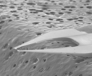
In an effort to improve the spatial resolution and frequency response of hot-wire anemometry, nanoscale thermal anemometry probes (NSTAP) were developed at Princeton (Kunkel, Arnold & Smits Reference Kunkel, Arnold and Smits2006; Bailey et al. Reference Bailey, Kunkel, Hultmark, Vallikivi, Hill, Meyer, Tsay, Arnold and Smits2010; Vallikivi et al. Reference Vallikivi, Hultmark, Bailey and Smits2011; Vallikivi & Smits Reference Vallikivi and Smits2014). These probes were made using microelectromechanical systems techniques and yielded ribbon-shaped sensors with a typical width  $w=2\ \mathrm {\mu }$m, thickness
  $t=0.1\ \mathrm {\mu }$m and length
  $\ell$ of either 60 or
  $30\ \mathrm {\mu }$m (see figure 9a). The sensors, therefore, have characteristic lengths approximately 10 times smaller than conventional hot wires, and as evident from figure 9(b) they also have a typical frequency response approximately 10 times higher. The square-wave results shown in this figure were supported by Hutchins et al. (Reference Hutchins, Monty, Hultmark and Smits2015) in their experiments in the Princeton SuperPipe, where the response of a standard hot-wire probe (
 $\ell =500\ \mathrm {\mu }$m,
  $d=2.5\ \mathrm {\mu }$m) was compared with that of an NSTAP probe (
 $\ell =60\ \mathrm {\mu }$m,
  $w=1\ \mathrm {\mu }$m,
  $t=0.1\ \mathrm {\mu }$m). The results given in figure 10 confirm the superior response of the NSTAP at higher frequencies.

Figure 9. Configuration and performance of NSTAP ( $\ell =60\ \mathrm {\mu }$m,
  $w=1\ \mathrm {\mu }$m,
  $t=0.1\ \mathrm {\mu }$m). (a) Scanning electron microscope images. The probe is mounted on a wax substrate (seen in the background) for imaging. From Vallikivi et al. (Reference Vallikivi, Hultmark, Bailey and Smits2011). (b) Temporal response of the NSTAP at different ambient air pressures. Top panel: square-wave response. Bottom panel: attenuation in signal with frequency (Bode diagram), where 0 dB indicates unity gain (estimated using square-wave response). From Vallikivi & Smits (Reference Vallikivi and Smits2014) with permission.

Figure 10. Comparison of the transfer function  $\chi _e$ for the same anemometer, but different probes: (grey) standard probe CTA2 at
  $y^+ \approx 80$; (black) NSTAP at
  $y^+ \approx 29$ (
 $\tau _c = 3.7\ \mathrm {\mu }$s). Standard probe dimensions
  $\ell =0.5$ mm,
  $d=2.5\ \mathrm {\mu }$m; NSTAP dimensions
  $\ell =60\ \mathrm {\mu }$m,
  $w=1\ \mathrm {\mu }$m,
  $t=0.1\ \mathrm {\mu }$m. Here,
  $\chi _e$ is a difference function, defined as the fractional variation of the premultiplied spectra for a given experiment. From Hutchins et al. (Reference Hutchins, Monty, Hultmark and Smits2015) with permission.
5.4. Log law for turbulence
NSTAP probes were used by Hultmark et al. (Reference Hultmark, Vallikivi, Bailey and Smits2012) in the SuperPipe at Reynolds numbers ranging from  $Re_\tau =1985$ to
  $98\,000$, with the corresponding value of
  $\ell ^+$ varying from 1.8 to 45.5. The results corrected according to (5.3) are shown in figure 11(a) in outer scaling and in figure 11(b) in inner scaling. Figure 11(a) plainly demonstrates the presence of a log law for turbulence over an extent that increases with Reynolds number. The solid line is given by
 \begin{equation} \overline{u^2}^+ = B_1 - A_1 \ln{(y/R)},\end{equation}
with  $A_1=1.25$ and
  $B_1=1.61$ ((4.2) with
  $V(y^+)=0$). At the highest Reynolds number, the log law starts at approximately
  $0.01R$, where the errors due to spatial filtering are negligibly small (
 $<0.5\,\%$). These measurements were the first to show unambiguously the presence of the log law in turbulence, which only became evident once
  $Re_\tau \ge 20 \times 10^3$. The extent of the log law increases with Reynolds number, and at the highest Reynolds number it spans more than 10 % of the pipe radius. This experiment also found that the region over which the log law in turbulence applies coincides with the region of the log law in the mean velocity, a very satisfying observation from the point of view of our scaling arguments and the attached eddy hypothesis. Hultmark et al. (Reference Hultmark, Vallikivi, Bailey and Smits2012) suggested that the appearance of this extended logarithmic variation marks the onset of the extreme Reynolds number range for pipe flow. Hultmark et al. (Reference Hultmark, Vallikivi, Bailey and Smits2013) then showed that this same result applies to rough wall pipe flows, and Marusic et al. (Reference Marusic, Monty, Hultmark and Smits2013) and Vallikivi, Hultmark & Smits (Reference Vallikivi, Hultmark and Smits2015b) found that it additionally describes high Reynolds number boundary layers, where Marusic et al. suggested a slightly modified slope (
 $A_1=1.26$) and found that the additive constant depends on the flow: for pipes
  $B_1=1.56$, and for boundary layers
  $B_1=2.30$. They were the first to propose that
  $A_1$ be named the Townsend–Perry constant to mark their contributions to the underlying theory.

Figure 11. Streamwise turbulence intensity distributions for pipe flow. SuperPipe data for  $Re_\tau =1985$ to 98 200. Corrected according to (5.3) (Smits et al. Reference Smits, Monty, Hultmark, Bailey, Hutchins and Marusic2011). The corresponding values of
  $\ell ^+$ varied from 1.8 to 45.5. (a) Profiles in outer layer scaling for
  $y^+>100$. The solid line is (5.6) with
  $A_1=1.25$ and
  $B_1=1.61$. (b) Profiles in inner layer scaling. For the four highest Reynolds numbers, the outer peak is located at a position
  $y^+ \ge 8\ell ^+$. Adapted from Hultmark et al. (Reference Hultmark, Vallikivi, Bailey and Smits2012) with permission.
It should be noted that the argument for the log law in turbulence put forward by Perry & Abell (Reference Perry and Abell1977) and Perry et al. (Reference Perry, Henbest and Chong1986) was based on a dimensional analysis of the energy spectra. For  $\overline {u^2}$ and
  $\overline {w^2}$ they postulated two overlap regions in wavenumber space: one between the outer scaled eddies and the wall-attached eddies; and one between the wall-attached eddies and the dissipative eddies. The first overlap region yields a
  $k^{-1}$ variation, and the second a
  $k^{-5/3}$ variation, where
  $k$ is the streamwise wavenumber. These results are in line with ‘classical’ expectations, but high Reynolds number experiments at Princeton failed to confirm such trends (Morrison et al. Reference Morrison, Jiang, McKeon and Smits2002, Reference Morrison, McKeon, Jiang and Smits2004; Rosenberg et al. Reference Rosenberg, Hultmark, Vallikivi, Bailey and Smits2013; Vallikivi, Ganapathisubramani & Smits Reference Vallikivi, Ganapathisubramani and Smits2015a), as did the most recent measurements in the Melbourne tunnel (Hwang, Hutchins & Marusic Reference Hwang, Hutchins and Marusic2021). It appears that the existence of a well-developed
  $k^{-1}$ spectrum is not a necessary condition for the presence of a logarithmic wall-normal dependence of the turbulence intensity. Hwang et al. (Reference Hwang, Hutchins and Marusic2021) also suggested, based on their analysis of the data, that the Townsend–Perry constant is weakly dependent on Reynolds number.
5.5. Inner and outer peaks
Consider now the SuperPipe results in inner scaling shown in figure 11(b). The first significant observation is with regard to the presence of the outer peak, which is clearly evident for  $Re_\tau \ge 20\,000$. At the location of the outer peak (
 $y=y_o$) the correction for spatial filtering at the highest Reynolds number was approximately
  $2.4\,\%$, and at
  $y^+=0.5y_o$ the correction was approximately
  $3.1\,\%$, so that these observations on the appearance of an outer peak were the first that were not compromised by spatial filtering.
The second significant observation from figure 11(b) is with respect to the inner peak. As might be expected, despite using NSTAP probes, the inner peak could not be accurately resolved at the higher Reynolds numbers even when corrected according to (5.3). This is illustrated in figure 12, where the magnitude of the inner peak is compared with other data. The DNS data by Lee & Moser (Reference Lee and Moser2015) follow a logarithmic rise in the peak value, in agreement with previous work (Metzger et al. Reference Metzger, Klewicki, Bradshaw and Sadr2001; Marusic & Kunkel Reference Marusic and Kunkel2003), and they proposed that
 \begin{equation} \overline{{u^2}_p}^+ = a_1 + b_1 \ln(Re_\tau),\end{equation}
with  $a_1=3.66$ and
  $b_1 = 0.642$. The hot-wire data taken in the Melbourne tunnel by Marusic et al. (Reference Marusic, Chauhan, Kulandaivelu and Hutchins2015) with
  $\ell ^+ \approx 24$ is also shown, together with the same results corrected according to (5.3). The agreement of the corrected data with (5.7) is impressive, which might be taken as indirect support for the correction used here. For the lower Reynolds numbers the corrected SuperPipe data from Hultmark et al. (Reference Hultmark, Vallikivi, Bailey and Smits2012) agrees well with (5.3) but then diverges noticeably for
  $Re_\tau >10\,000$. This is also true for the corrected HRTF boundary layer data by Vallikivi et al. (Reference Vallikivi, Hultmark and Smits2015b), where the divergence occurs for
  $Re_\tau >5000$. These trends are unlikely to be due to any uncertainty in the correction method, since for the NSTAP probes the correction for
  $Re_\tau < 40\,000$ was smaller than that applied to all of the Marusic et al. data. Monkewitz (Reference Monkewitz2021) recently suggested that there could be some blockage effects caused by the NSTAP support system, and this may indeed be the case because for
  $Re_\tau \ge 10\,000$ the inner peak is very close to the wall (for the HRTF data
  $y_p<0.1$ mm and
  $y_p/\ell < 1.66$). Finally, we see that the PIV data from the CICLoPE pipe flow facility (Willert et al. Reference Willert, Soria, Stanislas, Klinner, Amili, Eisfelder, Cuvier, Bellani, Fiorini and Talamelli2017) also shows some divergence at the higher Reynolds numbers, but this trend is likely due to spatial filtering, which was reported to be
  $-7.5\,\%$ at the highest Reynolds number.

Figure 12. Reynolds number variation of inner peak magnitude. Data from Marusic et al. (Reference Marusic, Chauhan, Kulandaivelu and Hutchins2015) for matched  $\ell ^+ \approx 24$ (+, red); data from Marusic et al. (Reference Marusic, Chauhan, Kulandaivelu and Hutchins2015) corrected according to (5.3) (+); SuperPipe NSTAP data from Hultmark et al. (Reference Hultmark, Vallikivi, Bailey and Smits2012) (
 $\bullet$, royal blue); HRTF NSTAP data from Vallikivi et al. (Reference Vallikivi, Hultmark and Smits2015b) (
 $\blacksquare$, grey); CICLoPE PIV data from Willert et al. (Reference Willert, Soria, Stanislas, Klinner, Amili, Eisfelder, Cuvier, Bellani, Fiorini and Talamelli2017);
  $\diamond$, channel flow DNS from Hoyas et al. (Reference Hoyas, Oberlack, Alcántara-Ávila, Kraheberger and Laux2022);
  $\vartriangle$, channel flow DNS from Lee & Moser (Reference Lee and Moser2015); ———
 $, u2p+= 3.66 + 0.642$ ln(Re
 $\tau$) (proposed by Lee & Moser).
In an effort to resolve these issues, NSTAPs were brought to the Melbourne wind tunnel, where the boundary layer is approximately 350 mm thick. The experiment therefore enabled unprecedented spatial resolution, so that even at the highest Reynolds number ( $Re_\tau = 20\,000$) measurements could be made in the near-wall region while maintaining
  $\ell ^+<3.5$. The profiles of
  $\overline {u^2}^+$ are shown in figure 13(a), and the inner peak magnitude indeed displayed the expected logarithmic variation with Reynolds number, as shown in figure 13(b). For the experimental and DNS data given in this figure, the variation is well represented by (5.7) with
  $a_1=3.54$ and
  $b_1 = 0.646$, very close to the values proposed by Lee & Moser (Reference Lee and Moser2015). This logarithmic growth in the inner peak magnitude remains to be verified at even higher Reynolds numbers, and recently Chen & Sreenivasan (Reference Chen and Sreenivasan2021) have argued that there must be a finite limit to its growth. This remains a topic for future investigation. Also, Smits et al. (Reference Smits, Hultmark, Lee, Pirozzoli and Wu2021) have proposed that the growth of the inner peak can be related to the wall stress fluctuations, which are influenced by the very large-scale motions in the outer flow (Marusic, Mathis & Hutchins Reference Marusic, Mathis and Hutchins2010; Mathis et al. Reference Mathis, Marusic, Chernyshenko and Hutchins2013; Agostini & Leschziner Reference Agostini and Leschziner2018; Marusic et al. Reference Marusic, Chandran, Rouhi, Fu, Wine, Holloway, Chung and Smits2021). On the basis of DNS data, Smits et al. concluded that only the contribution due to large-scale motions was Reynolds number dependent, and so the scaling in the near-wall region can be split into one function of
  $y^+$ and another for
  $Re_\tau$; that is, for
  $y^+ \le 20$,
 \begin{equation} \overline{u^2}^+ = f _1(Re_\tau ) f_2( y^+).\end{equation}
The outer limit for this scaling grows with Reynolds number, and the data by Samie et al. (Reference Samie, Marusic, Hutchins, Fu, Fan, Hultmark and Smits2018) suggest that it reaches out to at least  $y^+ \approx 50$ at
  $Re_\tau = 20\,000$.

Figure 13. (a) Streamwise turbulence intensity in boundary layers for  $Re_\tau =6123, 10\,100, 14\,680, 19\,680$. Data obtained using NSTAP in the Melbourne wind tunnel with
  $\ell ^+ = 2.5$ to 3.5. (b) Dependence of inner peak magnitude on Reynolds number. Here: NSTAP (
 $\bullet$); DNS of turbulent boundary layer from Sillero, Jiménez & Moser (Reference Sillero, Jiménez and Moser2013) (
 $\circ$); DNS of channel flow from Lozano-Durán & Jiménez (Reference Lozano-Durán and Jiménez2014) (
 $\Box$); , DNS of channel flow from Lee & Moser (Reference Lee and Moser2015) (
 $\triangledown$);
  $\overline {u^2}_p^+ = 3.54 + 0.646 \ln (Re_\tau )$ (——–);
  $\overline {u^2}_p^+ = 3.66 + 0.642 \ln (Re_\tau )$ (– – – –). From Samie et al. (Reference Samie, Marusic, Hutchins, Fu, Fan, Hultmark and Smits2018) with permission.
5.6. Mesolayer
We have considered the attributes of the inner and outer peaks, but there is a region that lies between, often called the mesolayer, covering approximately the same region where the mean velocity profile is best described by a power law (3.1), that is, the region defined by  $50 < y^+ < 300$. As noted by Vallikivi et al. (Reference Vallikivi, Ganapathisubramani and Smits2015a), the concept of a mesolayer was initially introduced by Long & Chen (Reference Long and Chen1981), and developed more fully by Afzal (Reference Afzal1982), Afzal (Reference Afzal1984), Sreenivasan & Sahay (Reference Sreenivasan and Sahay1997), George & Castillo (Reference George and Castillo1997), Wosnik, Castillo & George (Reference Wosnik, Castillo and George2000) and Wei et al. (Reference Wei, Fife, Klewicki and McMurtry2005). Wei et al. (Reference Wei, Fife, Klewicki and McMurtry2005) described the mesolayer (layer III in their nomenclature) as a region where there is a balance between turbulent inertia (stress gradients), the viscous force and either the force due to the pressure gradient in pipes or the mean advection in boundary layers. With the exceptions of George & Castillo (Reference George and Castillo1997) and Wosnik et al. (Reference Wosnik, Castillo and George2000), these studies identify the mesolayer as a region where an intermediate wall-normal length scale emerges that increases as
  $\sqrt {Re_\tau }$, where this length scale is mostly identified with the location of the maximum in the shear stress (see, for example, Sreenivasan & Sahay Reference Sreenivasan and Sahay1997).
Vallikivi et al. (Reference Vallikivi, Ganapathisubramani and Smits2015a) proposed bounds on the mesolayer that were different from those determined in previous studies. The lower bound was marked by the location where two peaks emerge in the premultiplied spectra, the ‘inner’ one corresponding to the large-scale motions and the ‘outer’ one corresponding to the very large-scale motions or superstructures ( $y^+>50$ for the boundary layer and
  $y^+>67$ for the pipe). The energy associated with the outer spectral peak increases with distance from the wall, and its location acts as the outer bound for this region, which closely matches the start of the logarithmic regions in the mean flow and the variance. For the lower Reynolds numbers the location of the outer spectral peak appeared to follow the
  $\sqrt {Re_\tau }$ scaling proposed for pipes and boundary layers in previous studies, and where it closely tallies with the position of the maximum in the shear stress, but for
  $Re_\tau > 20\,000$ it went asymptotically to a more or less constant position (in viscous scaling).
Finally, it is interesting to note that the streamwise length scale associated with the outer spectral peak, inferred using Taylor's hypothesis, appears as an intermediate length scale that seems to scale with  $\sqrt {Re_\tau }$ in both pipes and boundary layers. Vallikivi et al. (Reference Vallikivi, Ganapathisubramani and Smits2015a) therefore suggested that the mesolayer may be identified with the emergence of a new streamwise length scale rather than a new wall-normal length scale, as suggested previously.
5.7. Revisiting earlier data
With respect to the measurements by Fernholz & Finley (Reference Fernholz and Finley1996), given earlier in figure 4, we can now assess the effects of spatial filtering by correcting the data using (5.3). The comparison is shown in figure 14. The effects of spatial filtering are rather minor for  $y^+>100$, and the outer peak remains clearly visible after the corrections are applied. Also, in the region where we would expect to see a logarithmic variation in
  $\overline {u^2}^+$ the effects of spatial filtering are almost negligible, and the agreement with (5.6) is very good for the highest Reynolds numbers. It is apparent that this landmark experiment already contained the information necessary to establish the log law for turbulence and the development of the outer peak, but at the time it was unfortunately constrained by the absence of a suitable correction method for the effects of spatial filtering.

Figure 14. Boundary layer data from Fernholz & Finley (Reference Fernholz and Finley1996): (a,c) uncorrected; (b,d) corrected; (a,b) inner scaling; (c,d) outer scaling (for  $y^+>100$ only). Symbols as in figure 4. The solid line is (5.6) with
  $A_1=1.26$ and
  $B_1=2.3$.
6. Future directions
6.1. Subminiature probe development
The development of NSTAP probes has obviously had a positive impact on our ability to measure turbulence at high Reynolds number. Le-The et al. (Reference Le-The, Küchler, van den Berg, Bodenschatz, Lohse and Krug2021) have recently constructed a similar set of free-standing probes with  $\ell =70\ \mathrm {\mu }$m,
  $w\approx 300$ nm and
  $t \approx 100$ nm, and Baradel et al. (Reference Baradel, Leon, Giani, Combette and Mery2021) have fabricated comparable probes with
  $\ell =60\ \mathrm {\mu }$m,
  $w\approx 200$ nm and
  $t \approx 1.5\ \mathrm {\mu }$m. We can therefore expect to see a growing use of such small probes in the coming years as they become more readily available. Here, we have reported their effectiveness in the context of measuring velocity fluctuations in wall-bounded flows, but they have also been successfully used in experiments on homogeneous isotropic turbulence in the Göttingen Variable Density Turbulence Tunnel, as shown in figure 15. With NSTAP, Taylor microscale Reynolds numbers up to 1600 were investigated. At the highest Reynolds number, the Kolmogorov scale
  $\eta$ was 19
  $\mathrm {\mu }$m (Bodenschatz et al. Reference Bodenschatz, Bewley, Nobach, Sinhuber and Xu2014), so that the 30
  $\mathrm {\mu }$m NSTAP had
  $\ell /\eta < 1.6$, thereby avoiding any issues due to spatial filtering. The NSTAP probes have also been employed to investigate the atmospheric surface layer using constant current operation, and because of the high-frequency response of the probes no compensation was necessary (Huang et al. Reference Huang, Brunner, Fu, Kokmanian, Morrison, Perelet, Calaf, Pardyjak and Hultmark2021). They have been used to quantify the errors due to finite probe size in grid turbulence (Ashok et al. Reference Ashok, Bailey, Hultmark and Smits2012) and turbulent jets (Sadeghi, Lavoie & Pollard Reference Sadeghi, Lavoie and Pollard2018), and to characterize the wake behind a horizontal-axis wind turbine at very high Reynolds numbers (Piqué, Miller & Hultmark Reference Piqué, Miller and Hultmark2020).

Figure 15. Measurements using NSTAP in the Göttingen Variable Density Turbulence Tunnel. (a) Third-order structure functions. Here,  $u'$ is the fluctuating velocity and
  $L$ the integral length scale. The straight black line is equal to
  $r=L$, the scaling predicted by K41 4/5th law. (b) Logarithmic derivative of the fourth-order structure function with respect to the separation. Even at the highest Reynolds numbers measured, there seems to be only a slow approach to a horizontal line that would correspond to power-law scaling. The solid horizontal line is the prediction by K41 4/5th law, and the dashed line the prediction of the model by She & Leveque (Reference She and Leveque1994). The inset shows an enlargement of the intersection region. From Sinhuber, Bewley & Bodenschatz (Reference Sinhuber, Bewley and Bodenschatz2017) with permission.
In addition, the NSTAP design has been extended to encompass a number of other applications (Fan et al. Reference Fan, Arwatz, Van Buren, Hoffman and Hultmark2015). Two-component velocity measurements were made possible with the development of the X-NSTAP (Fu, Fan & Hultmark Reference Fu, Fan and Hultmark2019; Byers et al. Reference Byers, Hultmark, Marusic and Fu2021), as illustrated in figure 16. Each of the crossed wires were of length  $\ell =60\ \mathrm {\mu }$m, and they were contained within a measurement volume measuring
  $42\ \mathrm {\mu }{\rm m} \times 42\ \mathrm {\mu }{\rm m} \times 50\ \mathrm {\mu }{\rm m}$, which is comparable to the smallest NSTAP where
  $\ell =30\ \mathrm {\mu }$m. Byers et al. (Reference Byers, Hultmark, Marusic and Fu2021) used this probe to make two-component velocity measurements near the centreline of the SuperPipe for Reynolds numbers in the range
  $102 \le Re_\lambda \le 411$ (
 $1800 \le Re_\tau \le 24\,700$) to examine the inertial subrange scaling of the longitudinal and transverse velocity components. Even at the highest Reynolds number
  $\ell /\eta < 2.1$, so that spatial resolution issues were entirely avoided.

Figure 16. Configuration and performance of X-NSTAP. Measurement volume  $42\ \mathrm {\mu }{\rm m} \times 42\ \mathrm {\mu }{\rm m} \times 50\ \mathrm {\mu }{\rm m}$ (
 $\ell /\eta < 2.1$). (a) Scanning electron microscopy image of the X-NSTAP probe sensing elements. The two platinum sensing elements are shown perpendicular to each other to form an ‘X’. Each ribbon has
  $\ell =60\ \mathrm {\mu }$m,
  $w=1\ \mathrm {\mu }$m,
  $t=0.1\ \mathrm {\mu }$m. The wires are separated by a 50
  $\mathrm {\mu }$m thick spacer. From Byers et al. (Reference Byers, Hultmark, Marusic and Fu2021) with permission. (b) Non-dimensional dissipation rate on centreline of pipe flow. The symbols represent: the integration of longitudinal spectra (
 $\varepsilon _u$) (
 $\triangle$); the integration of transverse spectra (
 $\varepsilon _v$) (
 $\triangledown$); K41 4/5 law (
 $\Box$). Filled symbols are results from the X-NSTAP measurements and hollow/white symbols represent the corresponding parameter from Morrison, Vallikivi & Smits (Reference Morrison, Vallikivi and Smits2016). From Byers et al. (Reference Byers, Hultmark, Marusic and Fu2021) with permission.
6.2. Measuring temperature fluctuations
Another area of application for subminiature sensors is temperature measurement. A hot wire can be used to measure temperature fluctuations by operating it as a resistance thermometer, that is, by using a very small heating current, usually of order 1 mA. This ‘cold’ wire mode is not well-suited for constant temperature operation, and so the constant current mode is preferred. The primary issue is usually the frequency response. The NSTAP probes have a natural advantage in this respect because of their small thermal inertia, which typically improves the frequency response by an order of magnitude compared with conventional hot wires.
In a first step towards designing a cold-wire version of the NSTAP, Arwatz et al. (Reference Arwatz, Bahri, Smits and Hultmark2013) devised a lumped-capacitance-based model to characterize the sensor dynamic response. The model consists of three parts corresponding to the wire filament, stubs and prongs, and it accounts for the interaction and heat transfer among these elements. The model can predict the response of the probe based on its physical properties and dimensions, and it demonstrated that end-conduction effects are often more severe than previously thought and that they can lead to significant errors in measuring temperature.
These lessons were applied by Arwatz et al. (Reference Arwatz, Fan, Bahri and Hultmark2015) to develop an NSTAP probe specifically for temperature measurements, called T-NSTAP. The model had indicated that the probe performance could be improved in two specific ways. First, the thermal conductivity of the support structure was increased; instead of depositing a single platinum layer for the prongs, a 200 nm layer of gold was used because its thermal conductivity is more than four times higher. Second, the low-frequency response associated with end-conduction effects was improved by shortening the sensor support by 1 mm to reduce its thermal mass, and by increasing the length of the sensor to 200  $\mathrm {\mu }$m, approximately three times that of a regular NSTAP but still much shorter than conventional cold wires. Temperature measurements were then conducted in a heated grid-turbulence experiment with a cross-stream temperature gradient. The results given in figure 17(a) show that the T-NSTAP is substantially more accurate in measuring the variances than a conventional cold wire, which can underestimate the temperature variance by up to 25 % and the rate of scalar dissipation by up to 35 %. By comparing the spectra, as in figure 17(b), we see that the improvement spans the entire frequency range. Furthermore, when the model was used to correct the cold-wire data, a convincing degree of agreement was achieved between the two sets of data. The T-NSTAP has also proved to be remarkably robust. In preliminary measurements of temperature fluctuations in the atmospheric surface layer, Arwatz mounted six T-NSTAPs on booms fixed to the airframe of an ultralight airplane. The ultralight took off, flew over Lake Geneva at a variety of altitudes and then landed, without breaking a single probe (Smits & Hultmark Reference Smits and Hultmark2014).

Figure 17. (a) Temperature variance for a cold wire and a T-NSTAP at 6 m s $^{-1}$ (lower curves, circle symbol) and 9 m s
 $^{-1}$ (higher curves, square symbol). Here
  $x / M$ represents different cross-stream locations in a heated grid-turbulence set-up with a constant mean temperature gradient. From Arwatz et al. (Reference Arwatz, Fan, Bahri and Hultmark2015) with permission. (b) One-dimensional temperature dissipation spectra measured using a cold wire and T-NSTAP. From Arwatz et al. (Reference Arwatz, Fan, Bahri and Hultmark2015) with permission.
In a further demonstration of the capabilities of T-NSTAP, Williams et al. (Reference Williams, Van Buren and Smits2015) made measurements of temperature in a rough-wall turbulent boundary layer subject to weakly stable stratification at the same time as measuring two components of velocity using PIV to determine heat fluxes. The T-NSTAP flat frequency response exceeded 300 Hz, so that no compensation of any kind was necessary, permitting accurate measurements of the temperature fluctuations, heat fluxes and temperature dissipation spectra.
Finally, NSTAP probes are being developed for supersonic flow (S-NSTAP), and promising results have been obtained using (compensated) constant current operation at Mach numbers up to 2, both at the Bundeswehr University in Munich (Kokmanian et al. Reference Kokmanian, Scharnowski, Bross, Duvvuri, Fu, Kähler and Hultmark2019) and Aix Marseille Université (CNRS, IUSTI) in Marseille (Kokmanian et al. Reference Kokmanian, Barros, Hultmark and Dupont2021).
6.3. PIV and spatial resolution
In the context of high-resolution, high-accuracy measurement of turbulence, we have largely neglected any discussion of the role of PIV. Probably the most significant challenge to its success in this area is finding a way to use PIV so that the large- and the small-scale motions can be resolved at the same time. This conundrum was succinctly stated by Lavoie et al. (Reference Lavoie, Avallone, De Gregorio, Romano and Antonia2007). ‘The relatively coarse resolution of the PIV is somewhat typical of this measurement technique, where the scale resolution is a trade-off between zooming the image onto a small area to resolve small-scale motion, which can lead to a loss of global information and increases noise  $\ldots$, and capturing the region of the flow field that includes all relevant scales
  $\ldots$’. In this respect, Adrian (Reference Adrian1997) defined the dynamic spatial range of PIV as the field-of-view in the object space divided by the smallest resolvable spatial variation, so that a system with a large dynamic spatial resolution allows measurements of small-scale velocity variations embedded in larger-scale motions. It is clear that the limit on resolving the largest motions is set by the size of the field-of-view, and this limit is well understood. As to the limit on resolving the smallest scales in PIV, it is set by a combination of the thickness of the illuminating sheet and the size of the interrogation window, where the latter is generally a compromise between spatial resolution and data quality requirements in that smaller windows increase the number of spurious velocity vectors due to a reduction in the number of particles for each window (Lavoie et al. Reference Lavoie, Avallone, De Gregorio, Romano and Antonia2007).
To quantify and correct for the finite spatial resolution of PIV measurements, Lavoie et al. (Reference Lavoie, Avallone, De Gregorio, Romano and Antonia2007) developed an analytical method similar to the approach used by Wyngaard (Reference Wyngaard1968) for hot-wire anemometry. Their analysis was restricted to measurements in homogeneous isotropic turbulence, so the effects of spatial gradients were not considered. The main drawback of their approach, shared by Wyngaard's method, is that to correct any one component the spectrum for that component needs to be known. Since this almost always requires a matching hot-wire measurement, the method is restricted in its utility. Nevertheless, they noted that, for their case, the filtering effect of PIV on the spectrum for  $k_1 \eta >0.5$ was similar to a hot wire with
  $\ell = 2W$, where
  $W$ was the final (square) interrogation window size, so that the effects of spatial filtering in PIV in homogeneous isotropic turbulence is apparently more severe than that for hot wires. Unfortunately, this conclusion is difficult to translate to applications in wall-bounded flows. For example, in the usual set-up for measuring
  $\overline {u^2}$ the PIV window is oriented in the streamwise plane, whereas the hot wire would be oriented in the spanwise direction.
A good example of how the spatial resolution of PIV in wall-bounded flows might be estimated is given by the experiment by Willert et al. (Reference Willert, Soria, Stanislas, Klinner, Amili, Eisfelder, Cuvier, Bellani, Fiorini and Talamelli2017) in the CICLoPE pipe flow. Here, the missing energy due to PIV filtering was estimated using the one-dimensional transfer function of PIV for the streamwise spectrum proposed by Foucaut, Carlier & Stanislas (Reference Foucaut, Carlier and Stanislas2004), and applying this estimate to the hot-wire spectrum of a boundary layer obtained by Carlier & Stanislas (Reference Carlier and Stanislas2005). The difference between the integral of the filtered spectrum and that of the original spectrum was proposed as the best estimate of the missing energy. In fact, this approach is not so different from that used by Lavoie et al. (Reference Lavoie, Avallone, De Gregorio, Romano and Antonia2007), in that it also requires independent information on the spectral content of the signal.
These considerations address the estimates of the streamwise component, but one of the persistent problems with PIV is that the wall-normal and shear Reynolds stresses are often underestimated, even when the streamwise component is well resolved. This is most evident in high-speed, compressible flows (Williams Reference Williams2014; Williams et al. Reference Williams, Sahoo, Baumgartner and Smits2018), but it has been observed at all Mach numbers (see, for example, Bross, Scharnowski & Kähler Reference Bross, Scharnowski and Kähler2021). Recently, Aultman, Disotell & Duan (Reference Aultman, Disotell and Duan2022) used DNS to investigate the spatial resolution of PIV for the wall-normal components and clearly demonstrated the important role played by window size, and how spurious cross-correlations caused by the size of the illumination diameter and the local particle density set limits on the smallest acceptable window size.
7. Summary and concluding remarks
I hope to have shown that our current understanding of turbulent wall-bounded flows has been enabled by major advances in measurement techniques. Hot-wire anemometry, LDV and PIV have all contributed, often in a complementary manner. One of the major obstacles to progress in the past had been the filtering due to limited spatial resolution, which gave rise to well-founded doubts on some newly discovered features of high Reynolds number turbulence. Determining the inner and outer peak behaviour, and establishing the presence of the log law in turbulence, all depend crucially on either eliminating all spatial filtering, or keeping the filtering effects sufficiently small so that they can be convincingly corrected.
In hot-wire anemometry, the development of NSTAP, combined with the advent of purpose-built high Reynolds number facilities and a deeper understanding of spatial filtering, has now firmly established the log law in  $\overline {u^2}^+$ over approximately the same physical extent occupied by the log law in the mean velocity. We have also seen evidence for the log law in
  $\overline {w^2}^+$. This was first noted in the channel flow DNS data of Lee & Moser (Reference Lee and Moser2015), and then experimentally verified at higher Reynolds numbers by Zimmerman et al. (Reference Zimmerman2019) and Baidya et al. (Reference Baidya, Philip, Hutchins, Monty and Marusic2021). The latter data were obtained in the Melbourne tunnel for
  $Re_\tau$ up to
  $18\,400$, and with respect to (4.3) they found
  $A_2 \approx 0.27$ with
  $B_2$ displaying a slow logarithmic increase with Reynolds number.
In addition to the log law in turbulence, experiments have now verified the presence of an outer peak in  $\overline {u^2}^+$ at high Reynolds numbers in pipe and boundary layer flows, and unambiguously demonstrated the logarithmic growth in the inner peak with Reynolds number, at least for
  $Re_\tau$ up to approximately
  $20\,000$.
When the effects of spatial filtering cannot be avoided entirely, it seems that the method proposed by Smits et al. (Reference Smits, Monty, Hultmark, Bailey, Hutchins and Marusic2011) gives reasonable results for  $\ell ^+ \le 70$ and
  $y^+/\ell ^+ \ge 3$. Given this tool, it was possible to revisit the hot-wire data obtained in the DNW by Fernholz & Finley (Reference Fernholz and Finley1996). For
  $y^+>100$ the corrected data agreed in almost every respect with the NSTAP data obtained in the SuperPipe by Hultmark, Bailey & Smits (Reference Hultmark, Bailey and Smits2010) and Hultmark et al. (Reference Hultmark, Vallikivi, Bailey and Smits2012), and in the boundary layer tunnel at Melbourne University by Samie et al. (Reference Samie, Marusic, Hutchins, Fu, Fan, Hultmark and Smits2018). Therefore, the DNW experiments appear to be the first to establish the presence of the outer peak and the log law in turbulence. Unfortunately, they were not recognized as such at the time, primarily because of doubts regarding the effects of spatial filtering.
One of the more surprising conclusions from our survey of turbulence measurements is that experiments on the mean flow are simply not accurate enough to evaluate von Kármán's constant to better than  $0.40 \pm 0.02$. In addition, the inner peak in the streamwise turbulence increases logarithmically with
  $Re_\tau$, but at a rate that is considerably slower than expected from the attached-eddy model, and the origin of the outer peak remains to be explained (Smits Reference Smits2020). Also, spectral data on the streamwise velocity fluctuation point to the elusiveness of the asymptotic behaviour with increasing Reynolds number. For example, the slope of the inertial region asymptotes very slowly to
  $k^{-5/3}$, and no
  $k^{-1}$ region was found at the Reynolds numbers reported here. Furthermore, there is a pressing need for additional high Reynolds number experiments to examine more fully the behaviour of the other turbulence components that include measurements of spectra and higher-order moments, to build on the work by, for example, Meneveau & Marusic (Reference Meneveau and Marusic2013) and Baidya et al. (Reference Baidya, Philip, Hutchins, Monty and Marusic2021). Beyond isothermal flows, there is wide scope for new work to investigate flows with heat transfer where we know that the analogies between momentum and scalar transport are notably fragile.
New high Reynolds number experiments and computations are undoubtedly necessary to resolve these questions, as well as many others. It will be especially interesting to examine flow-specific trends by comparing pipe, channel and boundary layer behaviour. We have seen that high Reynolds number experiments in pipe and boundary layer flows are now routine, supported to a great extent by advanced measurement techniques. For many practical reasons, however, it seems unlikely that we will see comparable experiments on high Reynolds number channel flows. As to DNS, high Reynolds number boundary layer computations will be very expensive, but for channel and pipe flows the limits on Reynolds number are being pushed aggressively. For example, recent DNS of channel flow at  $Re^+=8000$ and
  $10\,000$ found a small region of log law in both the mean velocity and
  $\overline {{u^2}^+}$ (Yamamoto & Tsuji Reference Yamamoto and Tsuji2018; Hoyas et al. Reference Hoyas, Oberlack, Alcántara-Ávila, Kraheberger and Laux2022), and higher Reynolds numbers will soon be available. Figure 18 shows that for channel flow DNS the increase in Reynolds number is almost exactly logarithmic in time. In addition, recent DNS of pipe flow has reached Reynolds numbers of 5200 (Yao et al. Reference Yao, Schlatter, Rezaeiravesh and Hussain2021) and 6000 (Pirozzoli et al. Reference Pirozzoli, Romero, Fatica, Verzicco and Orlandi2021). Given this broadening scope of experiments and computations, the future looks exciting indeed.

Figure 18. A log–linear plot of Reynolds number achieved in DNS of channel flow (Kim, Moin & Moser Reference Kim, Moin and Moser1987; Moser, Kim & Mansour Reference Moser, Kim and Mansour1999; del Álamo et al. Reference del Álamo, Jiménez, Zandonade and Moser2004; Hoyas & Jiménez Reference Hoyas and Jiménez2006; Bernardini, Pirozzoli & Orlandi Reference Bernardini, Pirozzoli and Orlandi2014; Lozano-Durán & Jiménez Reference Lozano-Durán and Jiménez2014; Lee & Moser Reference Lee and Moser2015; Yamamoto & Tsuji Reference Yamamoto and Tsuji2018; Oberlack et al. Reference Oberlack, Hoyas, Kraheberger and Alcántara-Ávila2022).
Acknowledgements
Professors I. Marusic, M. Hultmark, J. Morrison and Dr L. Ding kindly provided comments on an earlier draft.
Funding
This work was supported by ONR under grants N00014-17-1-2309 and N00014-19-1-2301 (Program Manager P. Chang), and N00014-1-1-0533 (Program Manager R. Brizzolera).
Declaration of interests
The author reports no conflict of interest.


 Open access