A Decentralized Solution for Transmission Expansion Planning: Getting Inspiration from Nature


1
Escuela Técnica Superior de Ingeniería (ICAI), Instituto de Investigación Tecnológica, Universidad Pontificia Comillas, 28015 Madrid, Spain
2
University of Turin, 10124 Turin, Italy
3
Administración de Empresas y Estadística, Departamento Ingeniería de Organización, Escuela Superior de Ingenieros Industriales, Escuela Politécnica de Madrid, 28015 Madrid, Spain
4
Unidad Mixta Interdisciplinar de Comportamiento y Complejidad Social (UMICCS), 28015 Madrid, Spain
*
Author to whom correspondence should be addressed.
Energies 2019, 12(23), 4427; https://doi.org/10.3390/en12234427
Submission received: 18 September 2019
/
Revised: 14 November 2019
/
Accepted: 19 November 2019
/
Published: 21 November 2019
Abstract
:Transmission expansion planning is a problem of considerable complexity where classical optimization techniques are unable to handle large case studies. Decomposition and divide-and-conquer strategies have been applied to this problem. We propose an alternative approach based on agent-based modeling (ABM) and inspired by the behavior of the Plasmodium mold, which builds efficient transportation networks as result of its search for food sources. Algorithms inspired by this mold have already been applied to road-network design. We modify an existing ABM for road-network design to include the idiosyncratic features of power systems and their related physics, and test it over an array of case studies. Our results show that the ABM can provide near-optimal designs in all the instances studied, possibly with some further interesting properties with respect to the robustness of the developed design. In addition, the model works in a decentralized manner, using mostly local information. This means that computational time will scale with size in a more benign way than global optimization approaches. Our work shows promise in applying ABMs to solve similarly complex global optimization problems in the energy landscape.
1. Introduction
Transmission expansion planning (TEP) decides the optimal reinforcements for the transmission grid. Solving this problem presents considerable computational complexity, given the very high number of discrete variables that result from taking into account all the possible reinforcements. This issue has been exacerbated by the increase in renewable penetration. The variability of renewables could be balanced by using long-range transmission across geographical regions. This means that larger areas need to be planned in a coordinated manner. This is highly problematic, as computing time scales badly with size for these optimization problems. Decomposition, simplifications and other divide-and-conquer strategies have been proposed to tackle this issue, as explained below. A good overview of these issues is given in reference [1]. In this paper, we propose an alternative approach: agent-based modeling (ABM).
ABM is a consolidated methodology for creating computational models from a bottom-up perspective that is routinely applied in many disciplines, including ecology, the social sciences, economics, and biology [2]. The entities that comprise the system are explicitly represented in the model as agents that interact with each other and with the environment. These interactions are local, because they refer to agents and those they encounter in their proximity [3]. However, their interactions might lead to globally optimal design, such as in the cases of ant-colony behavior and slime mold growth, which have been shown to develop optimal networks [2]. In these biological systems, network development involves two phases: exploration and consolidation. The exploratory phase is characterized by the over-production of links between the core organism and the possible food sources. The consolidation phase, in turn, leads to the selection and positive reinforcement of the links that are used the most, while destroying or recycling the rest. The final network structure is likely to represent a context-specific balance between the need for efficient transport, low cost, and robustness.
The inspiration for our algorithm comes from reference [2]. In their article, which is based on biological experiments, the authors argue that the slime mold Physarum polycephalum creates a network that is efficient enough to compete with the real design of the railway system around Tokyo. The molds Plasmodium and Physarum have been shown to be able to solve many computational problems, such as finding the shortest path between two points [4], constructing hierarchies of planar proximity graphs [5], or executing basic logical computing schemes [5,6]. The molds are also capable of sketching a mathematical model of an adaptive network that solves a convoluted maze [2]. The key underlying mechanism supporting its success, in all these instances, is always this cycle of over-production of links and consolidation. This is precisely what we will imitate in our algorithm: the transmission lines that are used the most will be reinforced, while those that are not used will be discarded. Some studies tried to replicate the behavior of this specific slime mold by extrapolating its behavioral rules and simulating them in computer-based ABMs [7].
A succinct description of the basic ABM from reference [2] would be:
- Initialize a lattice of food pipes over the area under optimization.
- Calculate food flows.
- Update pipe capacities, increasing the capacities of the pipes that are used in full and decreasing the capacity of the pipes that are not used in full.
It should be noted that this algorithm is not directly applicable to TEP, given that:
- -
- A lattice cannot capture the discreteness of transmission lines (a transmission line should be considered as one investment, with a single capacity, from the start to the end node).
- -
- The physics of power flows is not considered.
These issues will be discussed in more detail below. In this paper, we present an ABM inspired by the behavior of the slime mold to solve TEP. Because ABMs rely on local information, they present a promising avenue to tackle TEP in large-scale systems.
The contributions of this paper are the following:
- We design an ABM to solve TEP. This ABM is inspired by the behavior of the slime mold and incorporating the physics of power flows and the idiosyncracies of the power system.
- We demonstrate its performance in a case study that shows that the resulting networks are consistently good across all case studies and might present some interesting properties with respect to robustness.
The rest of this paper is organized as follows. First, the remainder of this section describes TEP in more detail, as well as the existing works that have applied ABM to other problems in the energy landscape (to the extent of our knowledge, ours is the first application to TEP). Section 2 describes the mold-inspired ABM. Then, Section 3 details the case study that was developed to test the model. Section 4 presents the results and discusses them. Finally, Section 5 extracts conclusions.
1.1. Power Transmission Planning
TEP is one of the key decisions in power-systems design, with deep and long-lasting consequences on system performance. Transmission network planners must consider potential feedback from strategic market players [8] and decide whether to adopt a proactive or a reactive planning approach, which could lead to complicated hierarchical optimization and equilibrium problems (for an overview of TEP models under a liberalized market environment please refer to [9]). In general, transmission network planners must select which new lines to add to the network. The lines should be selected based on a cost criterion: the plan should minimize the sum of investment costs and operation costs. Investment costs refer to the cost of building the lines. Operation cost, in this context, refers to the costs of supplying demand with power. The network imposes constraints to the operation of the system, so that in general it is not possible to meet demand using the generator with the lowest cost. This is the case because all power flows are not possible—the maximum capacity of lines must be respected, and the laws of physics—which impose additional constraints known as Kirchhoff’s laws- should be abided too. New lines can enable the use of more efficient generators and make operation costs lower.
We use a mixed-integer programming formulation based on [10] that describes the impact of the network on physical power flows and system operation. We incorporate the possibility of taking into account different situations (regarding for instance fuel prices, hydro inflows or renewable generation) by means of the index ω. We reproduce a simplified version of the formulation below.
The objective function minimizes total annual cost, composed of investment and operation costs:
where is the investment cost, is the probability of the scenarios ω [pu], is the duration of the scenarios [h] and is the operation cost associated to the scenarios [€/h].
Investment [€] cost is calculated as the weighted sum of the cost of the planned investments. These are defined by decision variables , which describe the capacity of the transmission lines installed between nodes i and j using cable type c [MW]. The associated annualized investment cost of each unit of capacity between nodes i and j using cable type c is [€/MW], so investment cost takes the form:
It should be noted that this formulation allows installing fractions of a line at a proportion of their cost.
Operation cost is the sum of generation cost and not served power penalties:
where is the operation cost of an scenario, is the power generated at a node and scenario [MW], is the generation cost at a node and scenario [M€/MWh], is PNS (power not served at a node, which represents demand that could not be met) [MW] and is the penalty parameter associated to this unmet demand [M€/MWh].
A direct current (DC) power flow (DCPF) is a model that describes the physical power flows through the network by modeling a linear version of Kirchhoff’s laws. The first Kirchhoff’s law establishes that power must be balanced at every node (inputs equal outputs).
where is the flow between two nodes i and j through a cable c in a given scenario [MW] and is the demand at a node [MW].
is a particularly interesting dual variable: it corresponds to nodal price, the cost of providing one extra MW of energy at a given location i. Given network constraints, nodal prices are different at different nodes in the network.
The second Kirchhoff’s law or voltage law imposes that voltage differences added along a closed loop must be equal to zero. The DCPF formulation approximates this condition by applying it to a variable known as voltage angles only, and imposing that power flows must be proportional to the angle differences of the extremes of a line:
where are the voltage angles at nodes [rad] and represents the reactance of a circuit [pu], a parameter that describes the relative difficulty of sending power through a given cable. In general, reactance increases with distance (it is more difficult to send power) and decreases with capacity (it is easier to send power through lines with a higher capacity).
Generators must respect their constraints:
where and represent the minimum and maximum generation levels for a given generator.
Last, transmission lines must also respect their capacity limit:
where represents the maximum capacity that can be transferred between each pair of nodes [MW], and is calculated as the sum of the capacity installed taking into consideration the capacity of each cable type c, .
This simplified formulation presents the main features of the problem in order to give the reader an easily understandable overview of transmission expansion. We refer the reader to other publications (such as [11]) for a more detailed account.
TEP is a highly complex problem for numerous reasons: due to the high number of nodes in a network; and, due to the high amounts and different types of uncertainty decision makers have to face, which could be due to renewables [12], different investment options [13] or others. Taking into account other considerations such as integrating storage technologies [14] or Flexible Alternating Current Transmission Systems (FACTS) [15] into the TEP realm, further complicates the problem. Once we take into account the high number of nodes that appear in realistic power networks—of the order of hundreds or thousands. The number of connections between nodes that can be considered is therefore very large (several millions, considering that several cable types can be used). This leads to computational issues when applying classical optimization even in relatively small problem instances. This has historically led planners to resort to manual processes to plan their networks, which means the adoption of suboptimal solutions. The reference [11,16] presents strategies to cope with large problem sizes using optimization. The main idea in that work is to solve simpler versions of the problem instead of the full size. However, this paper takes a different approach: instead of simplifying the problem, we propose to keep the full complexity but modify the solution method. Instead of resorting to classical optimization, we use a biologically inspired algorithm to propose near-optimal designs: an algorithm based on a creature that is known to build near-optimal transportation networks.
The main advantage of our method is scalability: the algorithm uses local information only, as the slime mold can only sense its immediate surroundings regardless of the total size of the system. It should be noted, however, that power flows mostly should be calculated globally in order to abide the laws of physics, which apply to the system as a whole. We solve this issue by solving a suboptimization problem at each iteration step. This suboptimization problem is computationally light (all variables are linear) and can easily be integrated into the slime-mold algorithm. This is detailed in Section 2.
1.2. Agent-Based Modeling in Power Systems and Power Network Design
ABMs have already been adapted for use by the power systems research community. In particular, the IEEE Power Engineering Society (PES) formed a working group to investigate the drivers and benefits of ABMs in 2007 [17]. The conclusions of the working group were that ABMs could, if used appropriately, be used as a modeling approach and for building flexible software systems in the power systems domain. The working group highlighted that ABM is a very natural way of modeling actors in some systems such as power markets. In a market, actors have attributes (such as prices) and possible actions (such as bidding or production in a generation market) which they take independently considering the characteristics of the environment. ABMs can help understand the mechanics of such markets and the impact of changes in the actor attributes or behavior in the final outcome. The literature includes some examples of this type of study [18,19]. Among these recent applications, some of them study specific aspects such as the dispatching of wind energy [20], the modeling of demand elasticity through individual consumers [21,22], distributed generation [23], smart grids [24,25,26,27] or micro grids [28,29,30].
In addition to market studies, ABMs have been applied to monitoring and diagnostics, given that power systems have a complex structure that needs to be managed using a very large set of distributed data [31,32]. For these reasons, ABMs have been used in the context of reliability analyses, post-fault diagnosis (investigating the causes of a failure), or power system restoration [31,33,34]. Other applications deal with control and automation [23,25,26,28,30,35,36,37]. In addition, ABMs have been used as an optimization tool to calculate power flows [27] or the economic dispatch of generation units [38].
The application of ABMs to the distribution network has already produced some interesting applications that focus on a much smaller scale than the transmission network and consider urban networks [39,40,41]. In some cases, complex network considerations are introduced [41]. This emerging research has also introduced considerations on autonomous energy production systems [40] or microgrids [42]. However, the focus of this paper is the expansion of the transmission network at a country or regional level and not the distribution grid.
Although there has been a range of applications of ABMs to power systems, these have been focused on market simulation, control and automation. Applying ABMs to power systems planning has been far more limited, and exclusively focused on generation expansion, the generation companies’ decision to install new power plants. The use of ABMs for generation expansion is a result of the deregulation of the market, meaning that power expansion decisions are not made by a centralized system planner, but are decided by each company independently. In this context, it is intuitive to define generation companies as agents and use ABMs to study the impact of different expansion strategies. This has been done in works such as reference [43].
However, the authors could not find any literature that deals with the planning of the transmission network using ABMs. This is probably explained by the fact that, although the generation market was liberalized, the transmission grid is still planned in a central way in most countries given the related economies of scale [44]. We develop our model in the context of a liberalized generation market but with centralized transmission planning [45]. Therefore, the agent planning the grid is usually unique (the TSO or transmission system operator) and decides which new transmission assets to install based on considerations about the net social benefit derived for the system as a whole.
There are two references that deal with TEP and ABMs [46] and [47]. Reference [46] performs transmission expansion planning using an ABM to consider the generation companies’ behavior, but does not use ABM to plan the transmission expansion itself. Reference [47] uses an ABM to identify coalitions in the system—that is, groups of two or more agents that would benefit from acting together. In this paper, coalitions are more likely to build transmission lines if all coalition members receive increased benefits, which are assessed by means of the bilateral Shapley value.
Our work differs from these previous articles in two main ways. First, they consider a context where transmission is deregulated, while we assume that transmission planning is performed in a centralized way in accordance with the structure of the system in most countries. Second, they define agents that coincide with real agents in the system—generator companies, retailers or merchant line operators—that maximize their individual profits. Our agents do not coincide with real companies and do not maximize their individual profits. Our agents are an interpretation of the cells of P. plasmodium, which build a network to benefit the entire organism, which we assimilate to the whole power system. It is important to note that our aim is not to simulate the behavior of the entities that use the power transmission network but to create efficient power grid designs drawing inspiration from slime mold growth strategies. To do this, we use agents that, like the cells in the Plasmodium, use local information to build the links in the network to build designs in a decentralized manner. This aspect is key, as building designs based on local information leads to much smaller computational and memory resource needs. This local information is complemented with data about the global dynamics of the system that is introduced at each simulation step. Therefore, we conceive this algorithm as a support tool for a central planner: the final network result should be treated in the same way as the result from a classical optimization algorithm.
2. Materials and Methods
This section describes the mold-inspired ABM power-network model, which is one of the main contributions of this paper. The first part of this section explains the fundamental differences between the power network and other typical network problems, and the modeling challenges this entails. Then, we present our novel modeling framework, which, by combining ABM and classical optimization, allows us to tackle the TEP problem successfully.
2.1. How Power Networks Differ from Other Network Problems
The power grid presents additional features that make it fundamentally different, and more complicated than a plain transportation network design problem, which can be addressed by slime mold ABM in a straightforward way. These two features are as follows:
First, in a power network, load centers are usually geographically separated from power-generation locations due to geological and meteorological constraints. Therefore, we need to consider two different types of nodes: nodes where we have power generation, and nodes where we have power consumption (load centers). Hence, the first challenge for ABM to address transmission expansion planning is to be able to differentiate among these two types of nodes. Moreover, not all generation nodes are equivalent: cheap generation must be used preferentially. The algorithm should be able to integrate also price information into its mechanics.
Second, within a power network, energy flows are governed by physical laws: Kirchhoff’s laws. This makes power transmission fundamentally different from plain transportation problems. Replicating Kirchhoff’s laws and incorporating them into an ABM decision-making process is one of the main challenges addressed in this article. Each node has a state defined by a voltage (a voltage angle in the case of a linear power-flow model), and each line has a power flow that traverses it. Kirchhoff’s laws, as expressed in Section 3, link these voltages and currents. These laws mean that it is not possible to serve demand by sending power through the network in a cost-optimal way (that is, always from the cheapest source of energy). The OPF (optimal power flow) problem is the problem of finding the most efficient way of satisfying demand using existing generators considering their production costs and generation capacities, as well as the capacities of the existing transmission lines and the physical laws that govern the power flows. The formulation described in the section above corresponds to an OPF.
We tackle these challenges by combining standard optimization methods and ABM. The next section details our approach.
2.2. Transmission Expansion Planning Translated into Framework of Slime Mold-Inspired Agent-Based Model (ABM)
In this section, first, we point out how we addressed the difficulties of power grid expansion planning within an ABM framework. Then, we explain the applied methodology in detail. The two features, mentioned in Section 1.1, have been tackled as follows.
The two different types of nodes (generation and consumption) have been translated into the ABM as sources (generators) and sinks (loads), each with their different attributes corresponding to different variable generation costs and capacities. A standard slime-mold ABM is not capable of replicating the physical laws that govern power flows. While the most efficient way of taking food to the core of the slime mold is to follow minimum-distance paths, the most efficient use of power transmission lines is more difficult to assess and represent. This is due to the fact that the classic approach of ABM in the transport network takes only into account Kirchhoff’s First Law (inputs equal outputs at each node), but not the Second Law (voltage differences). One of our contributions is to incorporate power-flow considerations into the ABM framework. The OPF problem can be solved efficiently (after having approximated it by a standard linear optimization problem referred to as DC-OPF) as a standard optimization problem. We have modeled and solved the OPF using linear programming (LP) implemented in the General Algebraic Modeling System (GAMS) as optimization software. Detailed descriptions of the properties of the DC-OPF problem can be found for instance in [48]. The main results of this optimization are nodal prices ( in our formulation, corresponding to dual variables which can be defined as the cost of serving one additional megawatt (MW) of load at a given location), voltages and power flows. We follow the ODD documentation protocol [49] to develop the ABM. The model creates an efficient power network and is able to account operation and investment costs. It is coded in Netlogo 5.2 and we uploaded it to the website www.openabm.org. At each iteration, the ABM solves an OPF using linear programming using GAMS in order to make sure that the power flows respect Kirchhoff’s Laws and to get information such as line flows and nodal prices.
The model contemplates three kinds of agents: sinks (demand), sources (generators), and links (transmission lines). Sources generate a certain amount of electrical power (variable gen), according to a maximum generation capacity. Sources have an attribute type. This type affects their maximum capacity and production cost. It models different production technologies such as gas-fired, coal, nuclear or renewable generation. Sinks represent nodes where demand is located (urban or industrial centers). Trans-shipment nodes that neither have generation nor load could be represented as a source with zero generation capacity; or a sink with zero demand. However, without loss of generality but for the sake of simplicity, in the remainder of this paper we assume that there are no such trans-shipment nodes. Links represent transmission lines.
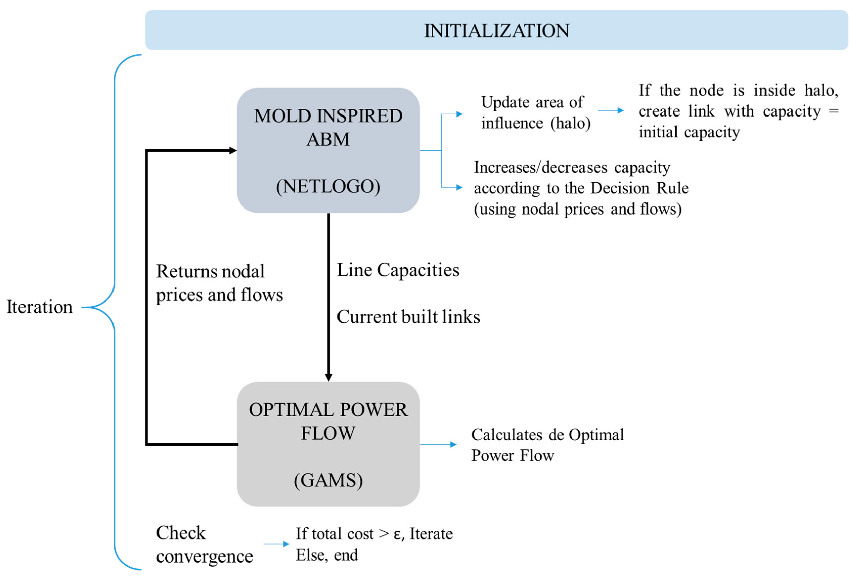
The ABM carries out an iterative process depicted in Figure 1 and described below. The process is based on demand centers having a growing area of influence where they can source for energy. New links are created within these areas of influence and are later reinforced or eliminated based on their efficiency. After an initialization, in which the number, location and type of the sinks and sources is determined, for each time step, the following processes are executed:
1. Update
Update the influence area of sources and sinks (we refer to this as halo), which defines the maximum area in which agents will contemplate the creation of links.
2. Create
Create new links.
3. Calculate power flows
This step is carried out by means of solving a DC-OPF problem, which incorporates Kirchhoff’s Laws. The optimal power flows respecting these laws, as well as nodal prices are calculated by GAMS and fed back into Netlogo.
4. Calibrate cables
Update cable capacity taking into account how efficient each transmission line currently is for the system. For this, we calculate the benefit brought by the transmission line and compare it to its investment cost. The potential benefit brought by the transmission line is approximated as its flow relative to its capacity times the difference in the nodal prices at its extremes. We can imagine this benefit as the profit that an investor would derive from using the line: if prices are different at the extremes, she could buy at the cheaper side and sell at the more expensive one. Hence, the potential benefit would be equivalent to the flow through the line times the difference in prices. This means that if power is sent from a cheaper to a more expensive area, the potential benefit is larger. Therefore, a network that is not well-connected (due to the lack of transmission lines) is more congested, which in turn leads to a higher nodal price difference. Hence, in highly congested networks it is indeed very beneficial to build new transmission lines. The ABM will build lines accumulating this benefit, and stop adding new lines if they are no longer beneficial to the network. The benefit is also larger if the capacity of the cable is used in full (that is, if the DC-OPF problem determines that the flow through the line equals its capacity). It should be noted that, in general, Kirchhoff’s Laws mean that the cable capacity is not used in full.
It should be noted that this potential benefit will be affected by the synergy among transmission lines installed and further eroded by the effect of transmission losses, so in general it is not a final benefit obtained from the line.
The single investment cost is defined as the link length [m] times the capacity of the line [MW] and times the cost of building a cable [K€/Km]:
If the difference between nodal prices (potential benefit) [€/MW] times the flow passing through the link [MW] is above the single investment cost of the cable, capacity is increased, reinforcing the transmission line. If not, then capacity is decreased. The nodal price is calculated in the optimization phase and is provided to the multi-agent programmable modeling environment Net Logo by GAMS.
In general, links that are used are reinforced (their capacity is increased); links that are not used weaken (their capacity is decreased). The speed for increasing or decreasing cables is determined via a parameter. If a cable weakens below a minimum capacity, it is deemed no longer economically viable and are eliminated.
5. Check convergence
The simulation ends if a stationary state is reached (transmission lines are not modified by two consecutive iterations).
3. Case-Study Description
In order to test the behavior of the slime-mold inspired model, we performed several experiments to analyze the results and the test the optimality of the solution. The ABM is applied to a set of random problem instances following the statistical characteristics of the European power system [50]. The model assumes standard costs and cable characteristics [44]. In each of the experiments, we consider 20 nodes in total (10 sink and 10 source buses) which are located randomly across a square with a side equivalent to 3000 km. This means that we have 10 buses, i.e., 10 sinks, at which we have demand that is exponentially distributed with an average value of 66 MW for each node. There are 10 generation buses, i.e., sources. The model considers different types of generation: wind, solar, hydro, nuclear, coal, gas (in particular, combined cycle gas turbine (CCGT), and open cycle gas turbine (OCGT)) and fuel-oil. The available maximum generation capacity at each generation bus, as well as its technology, is also sampled but according to the 2015 Spanish Energy Mix [51], which can be seen in Table 1 and are set.
The penalty for non-supplied energy (PNS, which represents unmet demand) is 1000 €/MWh. The agents can install transmission lines in full (at 100% of capacity), at a fraction of their capacity (less than 100%) or assuming several transmission lines can be installed in parallel (more than 100%).
The mold-inspired ABM, considers all potential combinations of new lines. This number of combinations corresponds to the binomial coefficient ( over 2), where corresponds to the total number of buses in the network. For our experiments with 20 nodes, this amounts to 190 different possible lines among nodes. For an increasing size of the network, this number of combinations becomes exceedingly large. However, during the iterative process, the mold-inspired ABM tries out many of these options but then eliminates them because they are not considered satisfactory alternatives. Only very few of these lines are consolidated. In particular, in the cases that we have run, around 11 or 12 different lines (out of the 190 possible ones) are actually built. The size of these lines (in terms of MW) and the length (in term of km) vary due to the location of the buses in each case. The cable characteristics considered can be seen in Table 2 below:
4. Results and Discussion
In this section we present the results of our method and analyze them in detail. We start out by comparing the newly developed mold-inspired ABM to classical optimization methods applied to the transmission expansion planning problem. Finally, we carry out a sensitivity analysis that explores the most relevant features of the model and how they are linked to the realistic conditions of the problem.
4.1. Comparing the Performance of Mold-Inspired ABM to Classical Optimization Methods
In this section we analyze the results of four separate simulations of Net Logo, which correspond to four samples of the random input data (node location and demand or capacity). The four simulations were obtained using our base case of the Spanish energy mix and the data described in the previous section.
We assess the quality of the results obtained with the mold-inspired ABM by comparing it to an objective benchmark calculated by standard optimization techniques. It should be noted that standard optimization can only be applied in relatively small case studies. As explained above, the main advantage of our ABM is that calculations are lighter and can be applied to problems of much larger sizes.
Table 3 contains the main cost results expressed in € of the four simulations, and compares those obtained: operating costs, investment costs, and total costs. When calculating total costs, we take into account the depreciation of the power system’s infrastructure and an annual discount rate. We use a 10% discount rate (i) for a 40-year depreciation (n), which translates into a factor of 0.10226 that is multiplied to the investment cost. This factor results from the application of a French (constant) amortization schedule:
First of all, we observe that operating costs are orders of magnitude lower than investment costs, which is a fact generally known in power systems. Second, we focus on the comparison of our ABM coded in Net Logo, and the TEP optimization model coded in GAMS. Since an optimization model assumes perfect information of all data, the obtained results correspond to the cost-minimal transmission expansion plan for a power grid. Table 3 shows that the total costs obtained by optimization are always below the total costs obtained by the ABM: the solution found by the ABM is suboptimal, as expected, the network it builds is not the perfect one. However, the ABM keeps a relatively close distance with respect to the optimal network: consistently between 16% and 19%.
Our ABM does not provide the globally optimal expansion solution; however, the behavior of the simulated mold approximates the optimal solution of a power grid reasonably well. The difference in costs is due to the fact that the mold’s behavior is based on increasing areas of interconnection between sources and sinks, while the GAMS solution treats the overall environment at once assuming perfect information. In particular, solving a TEP problem using optimization corresponds to a global planner with perfect information (about the location of demands and generators, as well as their technology, and distances between nodes), whereas our mold-inspired ABM mimics the behavior of a natural organism that only receives local information.
We could argue that, even though our results differ from the globally optimal results between 16% and 19%, the mold-inspired network might be more robust to possible changes in the system. For example, starting from both network solutions (the ABM solution and the globally optimal plan) and randomly adding a new node, it is very likely that the mold-inspired network is more robust to integrate this additional node in a cost-optimal way. This hypothesis seems reasonable given that this has been shown to be the case in other biological networks. However, it should be analyzed carefully to prove its validity in the context of power networks.
The ABM yields a network with more lines than the optimization model, which is the main factor that makes total cost rise. However, operating cost is cheaper in the ABM constructed network than in the cost-optimal network. The over-construction of power lines seems to have the advantage of leading to cheaper operating costs as well as increasing the robustness of the solution.
Our results show how the mold-inspired ABM is capable of creating, if not the globally optimal network, a reasonably good one, and one that might potentially be even more robust to possible changes and lead to lower operating costs. The fact that the mold-inspired ABM can achieve quasi-optimal designs using local information only is especially relevant for the TEP problem given that solving TEP using optimization is known to be a computationally heavy problem where solving large case studies is often unmanageable. In particular, in reference [11], Lumbreras et al. have developed an efficient large-scale optimization model for TEP. With this optimization approach, the authors have established a limit of several thousands of nodes as the maximum size that optimization can currently undertake with a satisfactory level of detail. One of the difficulties of TEP is the potentially very high amount of combinations of candidate lines. Such combinations in MIP lead to time and memory-intensive algorithms. The mold-inspired ABM approach presented in this paper could exceed the performance of such optimization models for large problems. In classical optimization, resources scale exponentially (or, rather, approximately exponentially) with the number of nodes, while in the case of ABM, resources increase approximately proportionately to the number of nodes. This advantage would arise from working with the local characteristics of the system for the investment decisions (and updating them with the global information coming from power flows at each iteration). This means that this algorithm could make it possible to solve potentially much larger instances than currently possible.
4.2. Sensitivity Analysis
A sensitivity analysis was performed to understand how changes in the environment affect the total cost of networks designed by the mold. We run each simulation 20 times for each parameter combination in order to obtain statistically sound results. The parameter space of the model is potentially very wide, hence, we decided to restrict our sensitivity simulations to a narrow parameter subset. The number of sinks and sources was fixed at 10, and we established an initial value for the transmission capacity of 10% of the total capacity of the transmission line. Each simulation run returns the investment cost, operating cost, and total cost of building and operating the network. The simulation also returns cable capacities and the sum of PNS during each simulation.
In this sensitivity analysis we explored the following parameter spaces: the relative penetration of cheap versus expensive generation technologies (that is, modifying the dominating generation technology), cable investment cost and the value of non-served power penalty.
4.3. Impact of the Technology Mix
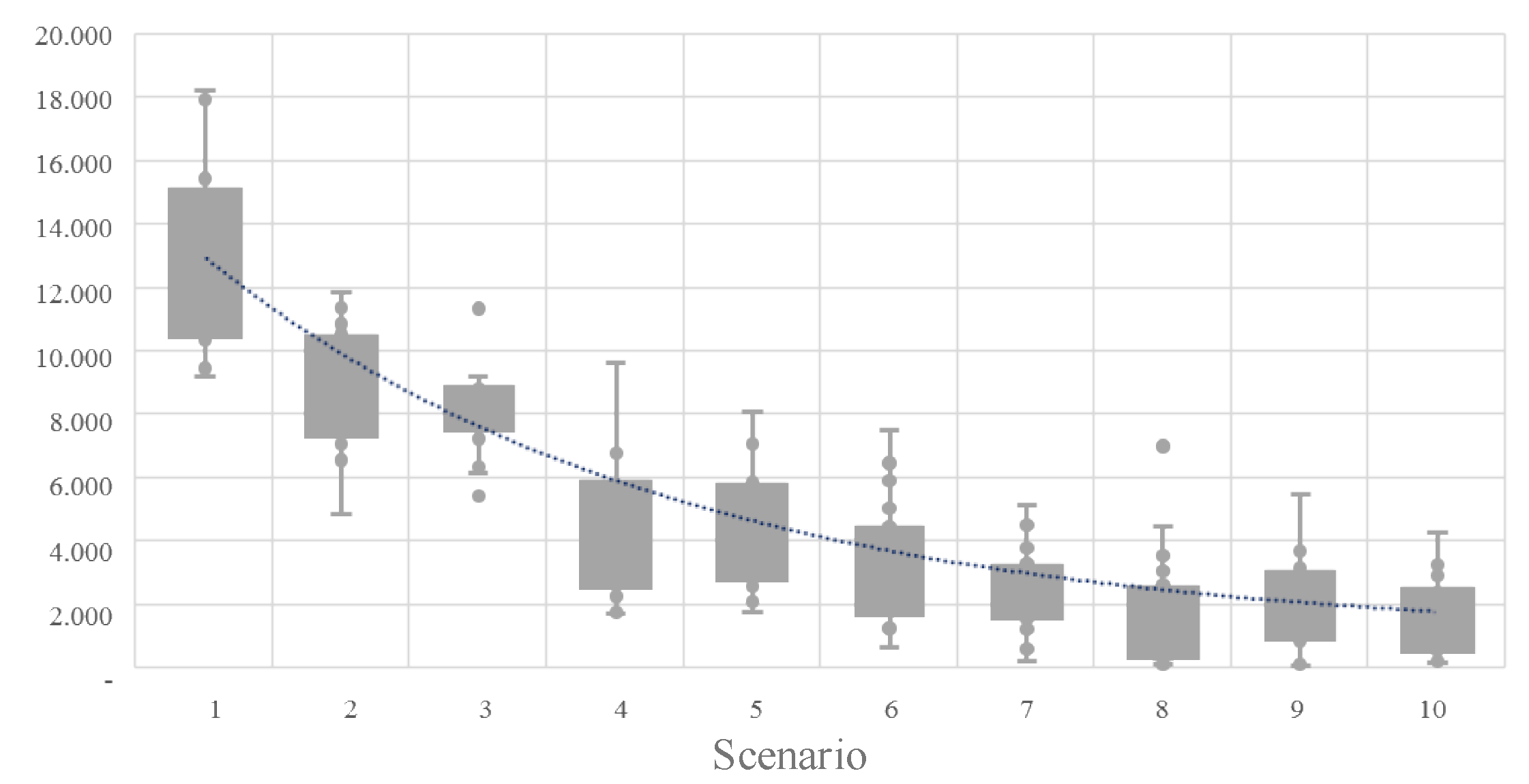
In this sensitivity analysis we assess how the technology mix of a power system impacts the obtained transmission expansion plan as well as investment and operating costs. To that end, we consider 10 scenarios of different technology mixes. The relative capacity penetration per scenario and for each technology is given by Table 4. Variable production costs of the technologies are as follows: 18 €/MWh for nuclear energy, 58.6 €/MWh for coal energy, 56.91 €/MWh for closed-cycle gas turbine, 100 €/MWh for open-cycle gas turbine, 1 €/MWh for wind energy, 3 €/MWh for solar energy and 3 €/MWh for hydroelectric energy.
It should be noted that we start with a system in which we predominantly have thermal peaking generation (scenarios 1–4). Then, thermal base-load technologies such as nuclear and coal are introduced in the technology mix up until a 50% penetration (scenarios 2–6). Afterwards, we introduce renewable energy sources such as hydro, solar and wind into the system up to 100% renewable penetration (scenarios 7–10). These scenarios can also be interpreted as going from expensive to cheaper operating costs.
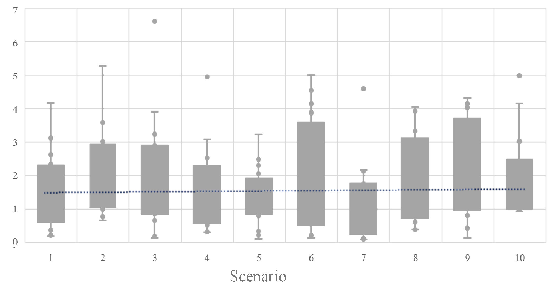
Figure 2 shows the distribution of the operating costs obtained for the 10 different power systems established in Table 4. As production costs decrease—going towards a cheaper renewable-only system—operating cost follows in an almost exponential decrease. However, investment costs decrease more slowly, as depicted in Figure 3. This is due to the fact that, even though the type of generation technology changes, the total amount of required MW demand does not; the same amount of power needs to be distributed within the network. The same applies to PNS, which remains stable through the different scenarios as observed in Figure 4.
Impact of Cable Investment Cost and Power Not Served (PNS) Penalty
Following our base case with the Spanish energy mix of 2015 and a PNS penalty of 1000 €/MW, we explore the impact of varying the cable investment costs from 50,000 €/km to 950,000 €/km in steps of 100,000 €/km (10 scenarios in total). In our results we observe that increasing cable investment costs naturally leads to an increase (among the 10 different scenarios) of investment costs obtained by the ABM. However, it is interesting to observe that the linear increase in cost parameters leads to an exponential increase in system operating costs, as depicted by Figure 5. This is due to the fact that, with higher cable investment costs, the total number of cables installed decreases, which leads to a higher amount of PNS within the system, which in turn leads to higher operating costs.
We carry out a similar simulation varying the PNS penalty. Starting from the base case of the 2015 Spanish energy mix, maintaining the cable cost constant at 50,000 €/km, we vary the penalty from 1000 €/MW to 10,000 €/MW in steps of 1000 €/MW. Our simulations indicate that as PNS increases, more transmission lines are built by the ABM. This is due to the fact that, since having PNS is growing increasingly expensive and less desirable within the system, more cables are built to avoid this penalty. A higher PNS penalty leads to more robust transmission grids. As a result, investment costs increase as well, since they are directly related to the cost of building each cable.
5. Conclusions
TEP presents considerable computational complexity, given the very high number of discrete variables that result from taking into account all the possible reinforcements. This issue has been exacerbated by the increase in renewable penetration and market integration, which call for planning large-scale regions in a coordinated manner. This is highly problematic, as computing time scales badly with size for these optimization problems. Decomposition, simplifications and other divide-and-conquer strategies have been proposed to tackle this issue. We propose an alternative approach by applying ABMs.
ABMs offer a very interesting property: they are based on local information, so their computation time scales relatively well with problem size although they approximate centralized solutions acceptably well. This advantage leads us to resort to ABMs as an optimization tool to tackle power network planning. For this, we adapt an existing ABM inspired on the behavior of slime mold, known to generate efficient transportation networks, to incorporate the specificities of the power system. This means introducing an optimization problem at each simulation step, although this optimization—which calculates the power flows through the network—is a benign problem compared to the transmission planning one.
The results using our mold-inspired model are all reasonable networks—albeit more expensive than those found by classical, MIP optimization. This difference in cost is not negligible but it is not unreasonable either, always below 20% in all cases analyzed. Biologically-inspired computation produced via ABM is capable of creating a reasonably good transmission network, and one that might potentially be even more robust to possible changes and lead to lower operating costs. The fact that the mold-inspired ABM can achieve quasi-optimal designs using local information only is especially relevant for the TEP problem given its complexity. This could be relevant for other problems where centralized planning is not possible, feasible or manageable. In this context, modified ABMs might provide an interesting alternative with a benign behavior for large problem sizes.
Author Contributions
Conceptualization: S.L., M.P. and I.B.; model: I.B., S.L., M.P., G.N., S.W.; methodology: S.L. and S.W.; validation and analyses: G.N., M.P., S.L.; writing: S.L., S.W., G.N.; resources and funding acquisition, S.W.
Funding
This research was partially funded by the Spanish Ministerio de Economía y Competitividad, grant number ENE2016-79517-R.
Conflicts of Interest
The authors declare no conflict of interest.
References
- Lumbreras, S.; Ramos, A. The new challenges to transmission expansion planning. Survey of recent practice and literature review. Electr. Power Syst. Res. 2016, 134, 19–29. [Google Scholar] [CrossRef]
- Tero, A.; Takagi, S.; Saigusa, T.; Ito, K.; Bebber, D.P.; Fricker, M.D.; Yumiki, K.; Kobayashi, R.; Nakagaki, T. Rules for biologically inspired adaptive network design. Science 2010, 327, 439–442. [Google Scholar] [CrossRef] [PubMed]
- Galán, J.M.; Izquierdo, L.R.; Izquierdo, S.S.; Santos, J.I.; del Olmo, R.; López-Paredes, A.; Edmonds, B. Errors and artefacts in agent-based modelling. J. Artif. Soc. Soc. Simul. 2009, 12, 1. [Google Scholar]
- Nakagaki, T. Smart behavior of true slime mold in a labyrinth. Res. Microbiol. 2001, 152, 767–770. [Google Scholar] [CrossRef]
- Adamatzky, A. Developing proximity graphs by Physarum polycephalum: Does the plasmodium follow the Toussaint hierarchy? LETT. Parallel Process. 2009, 19, 105–127. [Google Scholar] [CrossRef]
- Tsuda, S.; Aono, M.; Gunji, Y. Robust and emergent Physarum logical-computing. BioSystems 2004, 73, 45–55. [Google Scholar] [CrossRef]
- Takamatsu, A.; Takaba, E.G. Takizawa, Environment-dependent morphology in plasmodium of true slime mold Physarum polycephalum and a network growth model. J. Biol. 2009, 256, 29–44. [Google Scholar]
- Gonzalez-Romero, I.; Wogrin, S.; Gomez, T. Proactive transmission expansion planning with storage considerations. Energy Strategy Rev. 2019, 24, 154–165. [Google Scholar] [CrossRef]
- Gonzalez-Romero, I.C.; Wogrin, S.; Gomez, T. A Review on Generation and Transmission Expansion Co-Planning Models under a Market Environment. IET Gener. Transm. Distrib. 2019. Under Review. [Google Scholar]
- Binato, S.; Pereira, M.V.F.; Granville, S. A New Benders Decomposition Approach to Solve Power Transmission Network Design Problems. IEEE Trans. Power Syst. 2001, 16, 235. [Google Scholar] [CrossRef]
- Lumbreras, S.; Ramos, A. How to solve the transmission expansion planning problem faster: Acceleration techniques applied to Benders’ decomposition. IET Gener. Transm. Distrib. 2016, 10, 2351–2359. [Google Scholar] [CrossRef]
- Zhuo, Z.; Du, E.; Zhang, N.; Kang, C.; Xia, Q.; Wang, Z. Incorporating Massive Scenarios in Transmission Expansion Planning with High Renewable Energy Penetration. IEEE Trans. Power Syst. 2019. [Google Scholar] [CrossRef]
- Kim, W.W.; Park, J.K.; Yoon, Y.T.; Kim, M.K. Transmission Expansion Planning under Uncertainty for Investment Options with Various Lead-Times. Energies 2018, 11, 2429. [Google Scholar] [CrossRef]
- Wang, S.; Geng, G.; Jiang, Q. Robust Co-Planning of Energy Storage and Transmission Line with Mixed Integer Recourse. IEEE Trans. Power Syst. 2019, 34, 4728–4738. [Google Scholar] [CrossRef]
- Zhang, X.; Tomsovic, K.; Dimitrovski, A. Security constrained multi-stage transmission expansion planning considering a continuously variable series reactor. IEEE Trans. Power Syst. 2017, 32, 4442–4450. [Google Scholar] [CrossRef]
- Lumbreras, S.; Ramos, A.; Banez-Chicharro, F.; Olmos, L.; Panciatici, P.; Pache, C.; Maeght, J. Large-scale transmission expansion planning: From zonal results to a nodal expansion plan. IET Gener. Transm. Distrib. 2017, 11, 2778–2786. [Google Scholar] [CrossRef]
- McArthur, S.D.J.; Davidson, E.M.; Catterson, V.M.; Dimeas, A.L.; Hatziargyrio, N.D.; Ponci, F.; Funabashi, T. Multi-Agent Systems for Power Engineering Applications—Part I: Concepts, Approaches, and Technical Challenges. IEEE Trans. Power Syst. 2007, 22, 1743–1752. [Google Scholar] [CrossRef]
- Kiose, D.; Voudouris, V. The ACEWEM framework: An integrated agent-based and statistical modelling laboratory for repeated power auctions. Expert Syst. Appl. 2015, 42, 2731–2748. [Google Scholar] [CrossRef]
- Shafie-Khah, M.; Catalao, J.P.S. A Stochastic Multi-Layer Agent-Based Model to Study Electricity Market Participants Behavior. IEEE Trans. Power Syst. 2015, 30, 867–881. [Google Scholar] [CrossRef]
- Li, G.; Shi, J. Agent-based modeling for trading wind power with uncertainty in the day-ahead wholesale electricity markets of single-sided auctions. Appl. Energy 2012, 99, 13–22. [Google Scholar] [CrossRef]
- Thimmapuram, P.R.; Kim, J. Consumers’ Price Elasticity of Demand Modeling With Economic Effects on Electricity Markets Using an Agent-Based Model. IEEE Trans. Smart Grid 2013, 4, 390–397. [Google Scholar] [CrossRef]
- Karfopoulos, E.; Tena, L.; Torres, A.; Salas, P.; Jorda, J.G.; Dimeas, A.L.; Hatziargyriou, N.D. A multi-agent system providing demand response services from residential consumers. Electr. Power Syst. Res. 2015, 120, 163–176. [Google Scholar] [CrossRef]
- Divenyi, D.; Dan, A.M. Agent-Based Modeling of Distributed Generation in Power System Control. IEEE Trans. Sustain. Energy 2013, 4, 886–893. [Google Scholar] [CrossRef]
- Niese, A.; Lehnhoff, S.; Tröschel, M.; Uslar, M.; Wissing, C.; Appelrath, H.-J.; Sonnenschein, M. Market-based self-organized provision of active power and ancillary services: An agent-based approach for smart distribution grids. Complex. Eng. (CompEng) 2012, 2012. [Google Scholar] [CrossRef]
- Prostejovsky, A.; Merdan, M.; Schitter, G.; Dimeas, A. Demonstration of a multi-agent-based control system for active electric power distribution grids. In Proceedings of the Intelligent Energy Systems (IWIES), 2013 IEEE International Workshop, Vienna, Austria, 14 November 2013; pp. 76–81. [Google Scholar]
- Ross, K.J.; Hopkinson, K.M.; Pachter, M. Using a Distributed Agent-Based Communication Enabled Special Protection System to Enhance Smart Grid Security. IEEE Trans Smart Grid 2013, 4, 1216–1224. [Google Scholar] [CrossRef]
- Nguyen, C.P.; Flueck, A.J. A Novel Agent-Based Distributed Power Flow Solver for Smart Grids. IEEE Trans. Smart Grid 2015, 6, 1261–1270. [Google Scholar] [CrossRef]
- Dimeas, A.L.; Hatziargyriou, N.D. Operation of a multiagent system for microgrid control. IEEE Trans. Power Syst. 2005, 20, 1447–1455. [Google Scholar] [CrossRef]
- Colson, C.M.; Nehrir, M.H. Agent-based power management of microgrids including renewable energy power generation. In Proceedings of the Power and Energy Society General Meeting, Detroit, MI, USA, 24–28 July 2011; IEEE: Piscataway, NJ, USA, 2011; pp. 1–3. [Google Scholar]
- Dou, C.; Liu, B. Multi-Agent Based Hierarchical Hybrid Control for Smart Microgrid. IEEE Trans. Smart Grid 2013, 4, 771–778. [Google Scholar] [CrossRef]
- Davidson, E.M.; McArthur, S.D.J.; McDonald, J.R.; Cumming, T.; Watt, I. Applying multi-agent system technology in practice: Automated management and analysis of SCADA and digital fault recorder data. IEEE Trans. Power Syst. 2006, 21, 559–567. [Google Scholar] [CrossRef]
- Sharma, A.; Srivastava, S.C.; Chakrabarti, S. A multi-agent-based power system hybrid dynamic state estimator. IEEE Intell. Syst. 2015, 30, 52–59. [Google Scholar] [CrossRef]
- Koesrindartoto, D.; Sun, J.; Tesfatsion, L. An agent-based computational laboratory for testing the economic reliability of wholesale power market designs. In Proceedings of the Power Engineering Society General Meeting, San Francisco, CA, USA, 16 June 2005; IEEE: Piscataway, NJ, USA, 2005; pp. 2818–2823. [Google Scholar]
- Yan, X.; Shi, L.; Yao, L.; Ni, Y.; Bazargan, M. A multi-agent based autonomous decentralized framework for power system restoration. In Proceedings of the Power System Technology (POWERCON) International Conference, Chengdu, China, 20–22 October 2014; pp. 871–876. [Google Scholar]
- Xu, Y.; Liu, W.; Gong, J. Stable Multi-Agent-Based Load Shedding Algorithm for Power Systems. IEEE Trans. Power Syst. 2011, 26, 2006–2014. [Google Scholar]
- Nasri, M.; Farhangi, H.; Palizban, A.; Moallem, M. Multi-agent control system for real-time adaptive VVO/CVR in smart substation. In Proceedings of the Electrical Power and Energy Conference (EPEC), London, ON, Canada, 10–12 October 2012; IEEE: Piscataway, NJ, USA, 2012; pp. 1–7. [Google Scholar]
- Buse, D.; Sun, P.; Wu, Q.H.; Fitch, J. Agent-based substation automation. IEEE Power Energy Mag. 2003, 1, 50–55. [Google Scholar] [CrossRef]
- Kumar, R.; Sharma, D.; Sadu, A. A hybrid multi-agent based particle swarm optimization algorithm for economic power dispatch. Int. J. Electr. Power Energy Syst. 2011, 33, 115–123. [Google Scholar] [CrossRef]
- Fichera, A.; Pluchino, A.; Volpe, R. A multi-layer agent-based model for the analysis of energy distribution networks in urban areas. Phys. A Stat. Mech. Appl. 2018, 508, 710–725. [Google Scholar] [CrossRef]
- Volpe, R.; Frasca, M.; Fichera, A.; Fortuna, L. The role of autonomous energy production systems in urban energy networks. J. Complex Netw. 2016, 5, 461–472. [Google Scholar] [CrossRef]
- Fichera, A.; Volpe, R.; Frasca, M. Assessment of the energy distribution in urban areas by using the framework of complex network theory. Int. J. Heat Technol. 2016, 34, 430–434. [Google Scholar] [CrossRef]
- Kremers, E.; de Durana, J.G.; Barambones, O. Multi-agent modeling for the simulation of a simple smart microgrid. Energy Convers. Manag. 2013, 75, 643–650. [Google Scholar] [CrossRef]
- Gnansounou, E.; Dong, J.; Pierre, S.; Quintero, A. Market oriented planning of power generation expansion using agent-based model. In Proceedings of the Power Systems Conference and Exposition, New York, NY, USA, 10–13 October 2004; IEEE PES: Piscataway, NJ, USA, 2004; Volume 3, pp. 1306–1311. [Google Scholar]
- Lumbreras, S. Decision Support Methods for Large-Scale Flexible Transmission Expansion Planning. Ph.D. Thesis, Universidad Pontificia Comillas, Madrid, Spain, 2014. [Google Scholar]
- Hemmati, R.; Hooshmand, R.; Khodabakhshian, A. Comprehensive review of generation and transmission expansion planning. IET Gener. Transm. Distrib. 2013, 7, 955–964. [Google Scholar] [CrossRef]
- Motamedi, A.; Zareipour, H.; Buygi, M.O.; Rosehart, W.D. A Transmission Planning Framework Considering Future Generation Expansions in Electricity Markets. IEEE Trans. Power Syst. 2010, 25, 1987–1995. [Google Scholar] [CrossRef]
- Yen, J.; Contreras, J.; Klusch, M. Multi-agent approach to the planning of power transmission expansion. Decis. Support Syst. 2000, 28, 279–290. [Google Scholar] [CrossRef]
- Palma-Benhke, R.; Philpott, A.; Jofré, A.; Cortés-Carmona, M. Modelling network constrained economic dispatch problems. Optim. Eng. 2013, 14, 417–430. [Google Scholar] [CrossRef] [Green Version]
- Grimm, V.; Berger, U.; Bastiansen, F.; Eliassen, S.; Ginot, V.; Giske, J.; Goss-Custard, J.; Grand, T.; Heinz, S.K.; Huse, G.; et al. A standard protocol for describing individual-based and agent-based models. Ecol. Model. 2006, 198, 115–126. [Google Scholar] [CrossRef]
- EWEA. Wind in Power: 2014 European Statistics; EWEA: Brussels, Belgium, 2015. [Google Scholar]
- Lorscheid, I.; Heine, B.; Meyer, M. Opening the ‘black box’ of simulations: Increased transparency and effective communication through the systematic design of experiments. Comput. Math. Organ. Theory 2012, 18, 22–62. [Google Scholar] [CrossRef]
Figure 1.
Flowchart of the iterative process.

Figure 2.
Operating costs (€) for each scenario.

Figure 3.
Investment costs (€) for each scenario.

Figure 4.
Non-served power (MW) for each scenario.

Figure 5.
Operating costs (€) for each scenario when varying cable investment costs.


Table 1.
Characteristics of generators.
| Technology | Relative Penetration (%) | Capacity Lower Bound (MW) | Capacity Upper Bound (MW) | Marginal Cost (€/MWh) |
|---|---|---|---|---|
| Wind | 19.1% | 10 | 500 | 1.0 |
| Solar | 5.2% | 10 | 500 | 3.0 |
| Hydro | 11.1% | 10 | 500 | 3.0 |
| Nuclear | 21.7% | 1000 | 1500 | 18.0 |
| Coal | 20.3% | 500 | 100 | 58.6 |
| CCGT | 10.6% | 100 | 500 | 56.9 |
| OCGT | 12.0% | 100 | 500 | 100.0 |
Table 2.
Characteristics of transmission lines/cables.
| Basic Cable Characteristics | |
|---|---|
| Cable investment cost (€/km) | 50,000 |
| Initial cable capacity (MW) | 1000 |
| Reactance (ohm pu/km) | 0.008 |
Table 3.
Comparison of operating (Op) costs, investment (Inv) costs, and total costs between ABM approach in Net Logo, and transmission expansion planning (TEP) optimization approach in GAMS.
Table 3.
Comparison of operating (Op) costs, investment (Inv) costs, and total costs between ABM approach in Net Logo, and transmission expansion planning (TEP) optimization approach in GAMS.
| ABM | MIP | Δ (%) | |||||
|---|---|---|---|---|---|---|---|
| Op Cost (€) | Inv Cost (€) | Total Cost (€) | Op Cost (€) | Inv Cost (€) | Total Cost (€) | Total Cost | |
| 1 | 5912 | 2,851,647 | 297,522 | 2757 | 2,149,000 | 247,323 | 16.9% |
| 2 | 3556 | 5,156,841 | 530,894 | 3298 | 4,385,500 | 435,025 | 18.1% |
| 3 | 2027 | 5,609,869 | 575,693 | 1157 | 4,574,100 | 477,062 | 17.1% |
| 4 | 2755 | 3,602,599 | 311,157 | 3492 | 2,443,300 | 251,760 | 19.0% |
Table 4.
Percentage of capacity penetration of each technology for each of the scenarios.
| Scenario | % Wind | % Solar | % Hydro | % Nuclear | % Coal | % OCGT | % CCGT |
|---|---|---|---|---|---|---|---|
| 1 | - | - | - | - | - | - | 100 |
| 2 | - | - | - | - | 10 | 10 | 80 |
| 3 | - | - | - | - | 20 | 20 | 60 |
| 4 | - | - | - | 10 | 30 | 30 | 30 |
| 5 | - | - | - | 25 | 25 | 25 | 25 |
| 6 | 5 | 5 | 5 | 25 | 20 | 20 | 20 |
| 7 | 10 | 10 | 10 | 40 | 10 | 10 | 10 |
| 8 | 25 | 25 | 25 | 25 | - | - | - |
| 9 | 30 | 30 | 30 | 10 | - | - | - |
| 10 | 33.4 | 33.3 | 33.3 | - | - | - | - |
© 2019 by the authors. Licensee MDPI, Basel, Switzerland. This article is an open access article distributed under the terms and conditions of the Creative Commons Attribution (CC BY) license (http://creativecommons.org/licenses/by/4.0/).
Share and Cite
MDPI and ACS Style
Lumbreras, S.; Wogrin, S.; Navarro, G.; Bertazzi, I.; Pereda, M. A Decentralized Solution for Transmission Expansion Planning: Getting Inspiration from Nature. Energies 2019, 12, 4427. https://doi.org/10.3390/en12234427
AMA Style
Lumbreras S, Wogrin S, Navarro G, Bertazzi I, Pereda M. A Decentralized Solution for Transmission Expansion Planning: Getting Inspiration from Nature. Energies. 2019; 12(23):4427. https://doi.org/10.3390/en12234427
Chicago/Turabian StyleLumbreras, Sara, Sonja Wogrin, Guillermo Navarro, Ilaria Bertazzi, and Maria Pereda. 2019. "A Decentralized Solution for Transmission Expansion Planning: Getting Inspiration from Nature" Energies 12, no. 23: 4427. https://doi.org/10.3390/en12234427
Note that from the first issue of 2016, this journal uses article numbers instead of page numbers. See further details here.