
Comparing UAS LiDAR and Structure-from-Motion Photogrammetry for Peatland Mapping and Virtual Reality (VR) Visualization


1
Applied Remote Sensing Lab, Department of Geography, McGill University, Montreal, QC H3A 0G4, Canada
2
Flight Research Laboratory, National Research Council of Canada, 1920 Research Private, Ottawa, ON K1A 0R6, Canada
*
Author to whom correspondence should be addressed.
Drones 2021, 5(2), 36; https://doi.org/10.3390/drones5020036
Submission received: 15 April 2021
/
Revised: 5 May 2021
/
Accepted: 6 May 2021
/
Published: 9 May 2021
(This article belongs to the Special Issue Feature Papers of Drones)
Abstract
:The mapping of peatland microtopography (e.g., hummocks and hollows) is key for understanding and modeling complex hydrological and biochemical processes. Here we compare unmanned aerial system (UAS) derived structure-from-motion (SfM) photogrammetry and LiDAR point clouds and digital surface models of an ombrotrophic bog, and we assess the utility of these technologies in terms of payload, efficiency, and end product quality (e.g., point density, microform representation, etc.). In addition, given their generally poor accessibility and fragility, peatlands provide an ideal model to test the usability of virtual reality (VR) and augmented reality (AR) visualizations. As an integrated system, the LiDAR implementation was found to be more straightforward, with fewer points of potential failure (e.g., hardware interactions). It was also more efficient for data collection (10 vs. 18 min for 1.17 ha) and produced considerably smaller file sizes (e.g., 51 MB vs. 1 GB). However, SfM provided higher spatial detail of the microforms due to its greater point density (570.4 vs. 19.4 pts/m2). Our VR/AR assessment revealed that the most immersive user experience was achieved from the Oculus Quest 2 compared to Google Cardboard VR viewers or mobile AR, showcasing the potential of VR for natural sciences in different environments. We expect VR implementations in environmental sciences to become more popular, as evaluations such as the one shown in our study are carried out for different ecosystems.
1. Introduction
Peatlands cover a significant area globally (≈3%), and in particular of northern regions (e.g., ≈12% of Canada), and they have an increasingly important role in carbon sequestration and climate change mitigation [1,2,3,4]. Ongoing monitoring of peatlands over large spatial extents through the use of satellite-based Earth observation products is needed to understand their response to climate change (e.g., [5,6,7]). However, given their generally poor accessibility and the fine-scale topographic variation of vegetation microforms (often <1 m in height), satellite-based mapping requires validation from ground data (e.g., water table depth, species composition, biochemistry) [8,9]. Unmanned aerial systems (UAS) have shown potential for characterizing these ecosystems at fine scales [9,10,11]. In general terms, microtopographic features such as hollows and hummocks are key elements that are closely related to complex and associated hydrological, ecophysiological, and biogeochemical processes in peatlands [12]. Hummocks are elevated features composed of vascular plants overlaying mosses that consistently remain above the water table, while hollows are lower lying areas with primarily exposed mosses [13]. The multitemporal characterization of hollows and hummocks at submeter scales is key to validating satellite-derived products such as phenology tracking, net ecosystem exchange estimation, etc. [9].
To date, mapping microtopography with UAS has relied on two main technologies: light detection and ranging (LiDAR) and structure-from-motion (SfM) multiview stereo (MVS) photogrammetry (hereinafter referred to as SfM) with variable results for each technology (e.g., [14,15,16]). LiDAR is an active remote sensing technology that uses a pulsed laser generally between 800 and 1500 nm for terrestrial applications, to measure ranges, i.e., the variable distances from the instrument to objects on the surface of the Earth. It does so by measuring the exact time it takes for the pulses to return after they are reflected off objects or the ground [17]. In contrast, SfM is a passive remote sensing technique that uses overlapping offset photographs from which to reconstruct the landscape [18,19]. In forested areas, LiDAR pulses can penetrate the canopy and allow for the development of both canopy and surface terrain models [17], while SfM only provides a surface model of the highest layer, often the canopy, as seen from the photographs [20]. Comparatively, across ecosystems, SfM is shown to produce higher density point clouds than those from LiDAR. Previously in peatlands, mapping microtopography has been compared between UAS SfM and airborne LiDAR (e.g., [16]). Many studies have also employed airborne LiDAR for large-scale peatland assessments (e.g., [21,22,23,24,25,26]). Terrestrial laser scanning (TLS) has also been shown to successfully map microforms at very high spatial detail (e.g., [27]). However, no formal study has rigorously compared UAS LiDAR and SfM for mapping peatland microtopography.
Because peatlands are both fragile ecosystems and in general have poor accessibility, tools to remotely study, access, and visualize peatland structure in 3D are needed for advancing our understanding of their response to climate change. Although not a new technology [28], the recent advances in virtual reality (VR) [29], with its applications in medicine [30], conservation [31], geosciences [32,33], e-tourism [34,35], and education [36], among others, provide novel opportunities to study peatlands and other ecosystems remotely without disturbance [37]. VR is technology (hardware and software) that generates a simulated environment which stimulates a “sense of being present” in the virtual representation [38]. In contrast, augmented reality (AR) superimposes the virtual representation on the real world through glasses or other mobile digital displays, in turn supplementing reality rather than replacing it [39]. Thus, through VR, users experience an immersive experience of the field conditions in a cost-effective and repeatable manner. For instance, [29] showcases the advantages of VR, such as the quantification and analysis of field observations, which can be performed at multiple scales. While early implementations required extensive and expensive hardware, such as CAVE (CAVE Automatic Virtual Environments) [38], recent commercial grade VR systems that utilize improved head mounted displays (HMD), such as Oculus Rift, Sony PlayStation VR, HTC Vive Cosmos, etc., allow for outstanding visualization capabilities and sharing of scientific output through web-based platforms.
Our study aims to bridge the implementation of 3D models derived from UAS (LiDAR and SfM) and VR/AR visualization. Thus, our objectives are to (1) compare SfM and LiDAR point cloud characteristics from a peatland; (2) compare the representation of peatland microtopography from the SfM and LiDAR data; and (3) provide a qualitative evaluation of VR and AR usability and quality of visualization of the two point clouds. We further discuss the potential of VR in peatland research and provide web-based examples of the study area. While we primarily focus on VR due to the maturity of the technology and its suitability for scientific data visualization, we also briefly compare the point clouds in AR. To our knowledge, ours is the first study to compare microtopography between LiDAR and SfM for a peatland, in addition to investigating peatland VR/AR models derived from UAS data.
2. Materials and Methods
2.1. Study Area
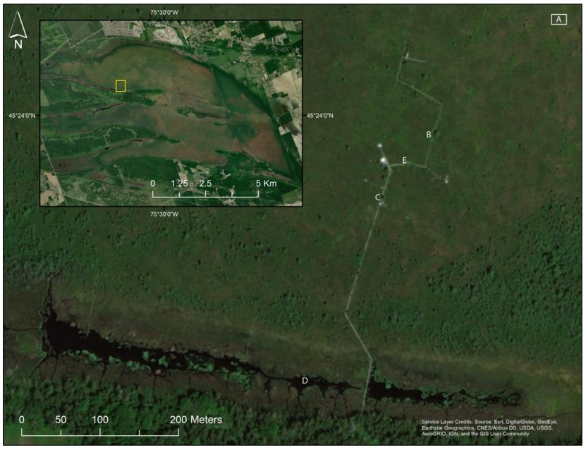
This study was carried out at Mer Bleue, an ≈8500 year-old ombrotrophic bog near Ottawa in Ontario, Canada (Figure 1). A bog is a type of peatland commonly found in northern regions. Bogs are acidic, nutrient-poor ecosystems, receiving incoming water and nutrients only from precipitation and deposition. Mer Bleue is slightly domed, with peat depth decreasing from >5 m across most its area to ≈30 cm along the edges. It has a hummock–hollow–lawn microtopography with a mean relief between hummocks and hollows of <30 cm [40,41]. While the water table depth is variable throughout the growing season, it generally remains below the surface of the hollows [42]. Malhotra et al. (2016) [43] found a strong association between spatial variations in vegetation composition, water table depth, and microtopography. However, the strength of the association varied spatially within the bog. Mosses, predominantly Sphagnum capillifolium, S. divinum, and S. medium (the latter two species were formerly referred to as S. magellanicum) [44] form the ground layer of the bog and can be seen exposed in low lying hollows. Vascular plants comprise the visible upper plant canopy of the hummocks (Figure 1). The most common vascular plant species are dwarf evergreen and deciduous shrubs (Chamaedaphne calyculata, Rhododendron groenlandicum, Kalmia angustifolia, Vaccinium myrtilloides), sedges (Eriophorum vaginatum), and trees (Picea mariana, Betula populifolia, and Larix laricina) [45]. Hummocks have been estimated to account for 51.2% and hollows for 12.7% of the total area [46]. Trees and water bodies (open and vegetated) around the margins of the peatland, which are heavily impacted by beavers, comprise the remaining classes.
2.2. Airframe
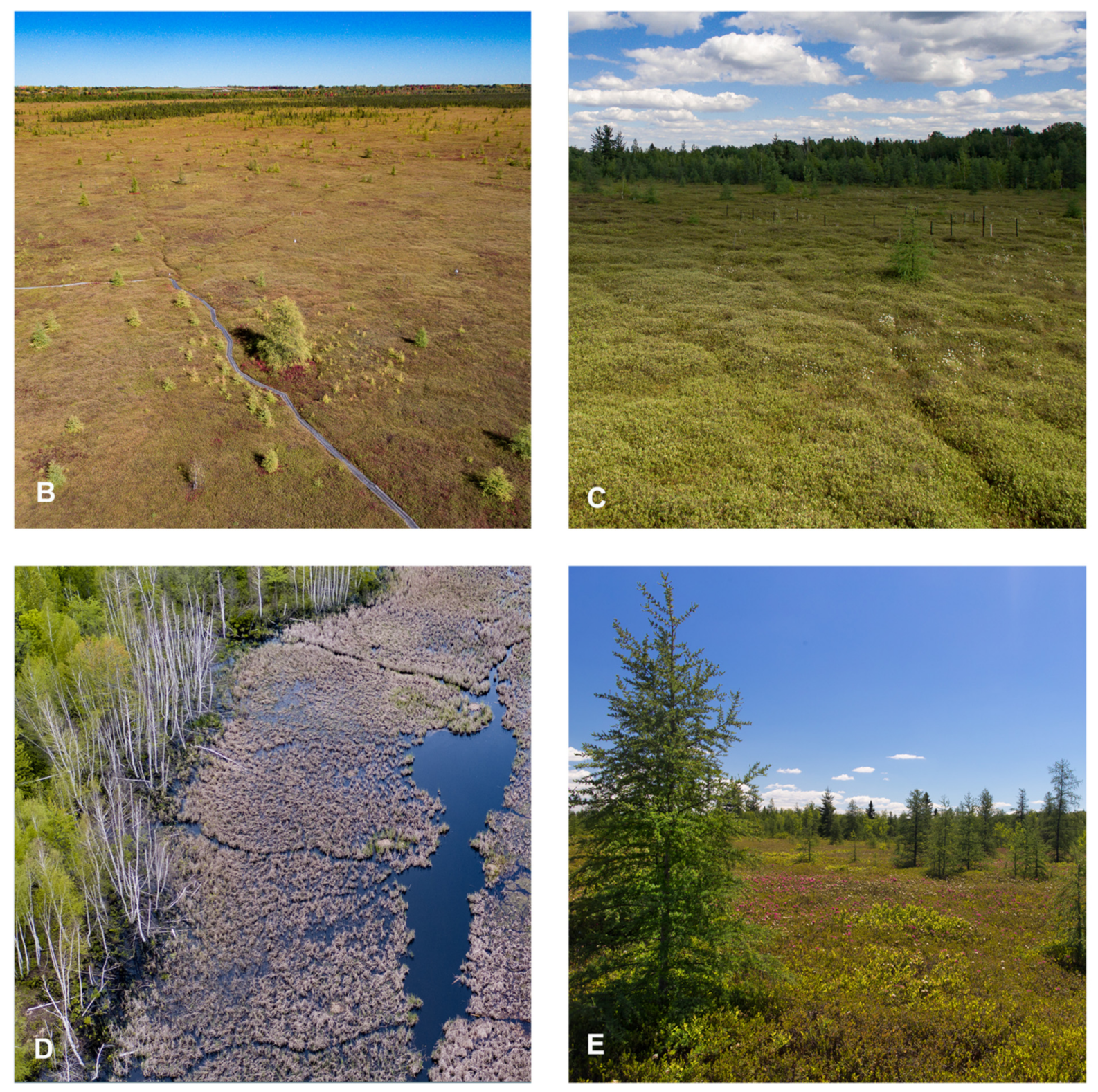
We used a Matrice 600 Pro (M600P) (DJI, Shenzhen, China) for both the RGB photograph and LiDAR acquisitions (Figure 2, Table A1). The M600P is a six-rotor unmanned aerial vehicle (UAV) with a maximum takeoff weight of 21 kg (10.2 kg payload) (DJI Technical Support, 2017) that uses an A3 Pro flight controller with triple redundant GPS, compass, and IMU units. We integrated a differential real-time kinetic (D-RTK) GPS (dual-band, four-frequency receiver) module with the A3 Pro [47] for improved precision of navigation [10]. For both datasets, DJI Ground Station Pro was used for flight planning and for the automated flight control of the M600P.
2.3. Structure from Motion Photogrammetry
A Canon 5D Mark III digital single-lens reflex (DSLR) camera with a Canon EF 24–70 mm f/2.8L II USM Lens set to 24 mm was used for the RGB photograph acquisition in June (Table A1). This is a full frame (36 × 24 mm CMOS) 22.1 MP camera with an image size of 5760 × 3840 pixels (6.25 μm pixel pitch). At 24 mm, the field of view of the lens is 84°. With the camera body and lens combined, the total weight was 1.9 kg. The camera was mounted on a DJI Ronin MX gimbal (2.3 kg) for stabilization and orientation control (Figure 2a). The camera’s ISO was set to 800 to achieve fast shutter speeds of 1/640 to 1/1000 s at f/14 to f/16. The photographs were acquired from nadir in Canon RAW, (.cr2) format and were subsequently converted to large JPG (.jpg) files in Adobe Lightroom® with minimal compression. Because the M600P does not automatically geotag the photographs acquired by third party cameras, geotags were acquired separately.
Geotagging was achieved through a postprocessing kinematic (PPK) workflow with an M+ GNSS module and Tallysman TW4721 antenna (Emlid, St. Petersburg, Russia) to record the position and altitude each time the camera was triggered (5 Hz update rate for GPS and GLONASS constellations) (Table A1). A 12 × 12 cm aluminum ground plane was used for the antenna to reduce multipath and electromagnetic interference and to improve signal reception. The camera was triggered at two second intervals with a PocketWizard MultiMax II intervalometer (LPA Design, South Burlington, VT, USA). A hot shoe adaptor between the camera and the M+ recorded the time each photograph was taken with a resolution of <1 µs (i.e., flash sync pulse generated by the camera). The setup and configuration steps are described in [48]. The weight of the M+ GNSS module, the Tallysman antenna, the intervalometer and cables were 300 g combined. Photographs were acquired from an altitude of 50 m AGL with 90% front overlap and 85% side overlap. With the aforementioned camera characteristics, i.e., altitude and overlap, the flight speed was set to 2.5 m/s by the flight controller. The total flight time required was ≈18 min.
Base station data from Natural Resources Canada’s Canadian Active Control System station 943020 [49] (9.8 km baseline) was downloaded with precise clock and ephemeris data for PPK processing of the M+ geotags. The open-source RTKLib software v2.4.3B33 [50] was used to generate a PPK corrected geotag for each photograph. A lever arm correction was also applied to account for the separation of the camera sensor from the position of the TW4721 antenna.
We used Pix4D Enterprise v4.6.4 (Pix4D S.A, Prilly, Switzerland) to carry out an SfM-MVS workflow to generate the dense 3D point cloud (Table A1). Unlike UAV integrated cameras with camera orientation written to the EXIF data, the DSLR photographs lack this information. However, these initial estimates are not necessary because during processing, Pix4D calculates and optimizes both the internal (e.g., focal length) and external camera parameters (e.g., orientation). In addition to the camera calibration and optimization in the initial processing step, an automatic aerial triangulation and a bundle block adjustment are also carried out [51]. Pix4D generates a sparse 3D point cloud through a modified scale-invariant feature transform (SIFT) algorithm [52,53]. Next, the point cloud is densified with an MVS photogrammetry algorithm [54]. For this comparison, we did not generate the raster digital surface model (DSM) through Pix4D (see Section 2.5).
SfM Point Cloud Accuracy
Two separate flights (≈12 min total flight time) with the same equipment described above were carried out ≈30 min earlier in a vegetated field, 300 m south of the primary bog study area. This field was located on mineral soil and therefore is less impacted by foot traffic than the fragile bog ecosystem. In an area of 0.2 ha, twenty targets to be used as check points were placed flat on the ground. Their positions were recorded with an Emlid Reach RS+ single-band GNSS receiver (Emlid, St Petersburg, Russia) (Table A1). The RS+ received incoming NTRIP corrections from the Smartnet North America (Hexagon Geosystems, Atlanta, GA, USA) NTRIP casting service on an RTCM3-iMAX (individualized master–auxiliary) mount point utilizing both GPS and GLONASS constellations. The accuracy of the RS+ with the incoming NTRIP correction was previously determined in comparison to a Natural Resources Canada High Precision 3D Geodetic Passive Control Network station, and it was found to be <3 cm X, Y, and 5.1 cm Z [55]. The photographs from the camera and geotags were processed the same way as described above with RTKlib and Pix4D up to the generation of the sparse point cloud (i.e., prior to the implementation of the MVS algorithm). Horizontal and vertical positional accuracies of the sparse 3D point cloud were determined from the coordinates of the checkpoints within Pix4D. The results of this accuracy assessment are used as an estimate of the positional accuracy of the SfM model of the study area within the bog where no checkpoints were available.
2.4. LiDAR
We used a LiAIR S220 integrated UAS LiDAR system (4.8 kg) (GreenValley International, Berkeley, CA, USA) hard mounted to the M600P in August (Figure 2b) (Table A1). The system uses a Hesai Pandar40P 905 nm laser with a ±2 cm range accuracy, a range of 200 m at 10% reflectivity, and a vertical FOV of –25° to +15° [56,57]. The Pandar40P is a 40-channel mechanical LiDAR that creates the 3D scene through a 360° rotation of 40 laser diodes. The majority of the lasers (channels 6–30) are within a +2° to –6° range of the FOV [58]. The integrated S220 system utilizes an RTK enabled INS (0.1° attitude and azimuth resolution) with an external base station and a manufacturer stated relative final product accuracy of ±5 cm. The system includes an integrated Sony a6000 mirrorless camera that is triggered automatically during flight. These JPG photographs are used to apply realistic RGB colors to the point cloud in postprocessing.
Two flights at 50 m AGL and 5 m/s consisting of 6 parallel flight lines (40 m apart) were carried out. Importantly, prior to the flight lines, two figure 8s were flown to calibrate the IMU. The same figure 8s were repeated after the flight lines prior to landing. Total flight time was ≈10 min. The LiAcquire software (GreenValley International, Berkeley, CA, USA) provided a real-time view of the point cloud generation.
LiAcquire and LiNAV were used for the postprocessing of trajectory data and the geotagging of the RGB photographs. The LiDAR360 software (GreenValley International, Berkeley, CA, USA) was then used to correct the boresight error, carry out a strip alignment, merge individual strips, and calculate quality metrics consisting of analyses of the overlap, elevation difference between flight lines, and trajectory quality.
2.5. Analysis
The open source CloudCompare Stereo v2.11.3 (https://www.danielgm.net/cc/) (accessed on 14 April 2021) software was used to analyze the point clouds (Table A1). After the initial positional difference between the point clouds was computed, the LiDAR point cloud was coarsely aligned to the SfM point cloud followed by a refinement with an iterative closest point (ICP) alignment. Each point cloud was detrended to remove the slope of the bog surface. The point clouds were then clipped to the same area and compared. Characteristics including the number of neighbor points, point density, height distribution, surface roughness (distance between a point and the best fitting plane of its nearest neighbors), and the absolute difference between point clouds were calculated. DSMs at 10 and 50 cm pixel sizes were also created from each dataset. CloudCompare was used to generate the DSMs rather than Pix4D and LiDAR360 respectively to ensure differences in the surfaces are not due to varying interpolation methodology between the different software. The average method with the nearest neighbor interpolation (in case of empty cells) was chosen for the rasterization of the point clouds.
To classify the hummocks and hollows, the DSMs were first normalized in MATLAB v2020b (MathWorks, Natick, MA, USA) by subtracting the median elevation in a sliding window of 10 × 10 m [59]. Hummocks were defined as having a height range 5–31 cm above the median and hollows as >5 cm below the median. These thresholds were defined on the basis of expert knowledge of the site. In the SfM data, this corresponded to the 55th–90th percentile of the height for hummocks and the bottom 38th percentile for hollows. In the LiDAR data, it corresponded to the 48th–71st percentile of the height for hummocks, and the bottom 40th percentile for hollows. A decision tree was used to assign the DSM pixels to hummock, hollow, and other classes based on their normalized height value.
To quantify the shape and compare the apparent complexity of the microforms from the SfM and LiDAR, we calculated the 3D Minkowski–Bouligand fractal dimension (D) of the surface of the bog [60]. The 3D fractal dimension combines information about an object/surface across different spatial scales to provide a holistic quantification of the shape [61]. The point clouds were converted to triangular meshes at rasterization scales of 10 and 50 cm in CloudCompare. The fractal dimension, D, was then calculated following the methodology described in [61]. The fractal dimension is a scale-independent measure of complexity. As defined by [62], fractals are “used to describe objects that possess self-similarity and scale-independent properties; small parts of the object resemble the whole object”. Here, D is a measure of the complexity of the bog surface as modeled by the triangular mesh objects from the SfM and LiDAR data sources. The value of D ranges from 0 to 3, with higher values indicating more complexity in the shapes. In this case, the complexity quantified by D is related to the irregularity pattern [61], with more regular shapes having lower values.
Lastly, empirical semivariograms were used to compare the scale dependence of the hummock–hollow microtopography to determine whether the scale of the vegetation pattern captured by the SfM and LiDAR datasets is similar. The spatial dependence of the height of the vegetation can be inferred from the semivariogram which plots a dissimilarity measure (γ) against distance (h). The range, sill, and nugget describe the properties of the semivariogram. The range indicates the spatial distance below which the height values are autocorrelated. The sill indicates the amount of variability and the nugget is a measure of sampling error and fine-scale variability. Previous application of empirical semivariograms to terrestrial LiDAR data from a peatland indicated the hummock–hollow microtopography had an isotropic pattern with a range of up to 1 m, and in sites with increased shrub cover, the range increased to 3–4 m [27]. The empirical semivariograms were calculated in MATLAB v2020b for a subset of the open bog that did not include boardwalks.
In order to generate the PLY files (i.e., Polygon file format, .ply) needed for VR and AR visualization, the horizontal coordinates (UTM) were reduced in size (i.e., number of digits before the decimal) using a global shift. In this case, 459,400 was subtracted from the easting and 5,028,400 from the northing. Binary PLY files were then generated with CloudCompare.
Both VR (Section 2.6) and AR (Section 2.7) visualizations were compared to a standard web-based 3D point cloud viewer as a baseline. We used a Windows server implementation of Potree v1.8 [63], a free open-source WebGL based point cloud renderer to host the point clouds (https://potree.github.io/) (accessed on 14 April 2021).The Potree Converter application was used to convert the LAS files (.las) into the Potree file and folder structure used by the web-based viewer for efficient tile-based rendering. In addition to navigation within the point cloud, user interactions include measurements of distance and volume and the generation of cross sections.
2.6. Virtual Reality Visualization
We tested the VR visualization of the point clouds with an Oculus Quest 2 headset (Facebook Technologies LLC, Menlo Park, CA. USA) (Table A1). The Oculus Quest 2 released in 2020, is a relatively low cost, consumer-grade standalone VR HMD. It has 6 GB RAM and uses the Qualcomm Snapdragon XR2 chip running an Android-based operating system. The model we tested had 64 GB of internal storage. The fast-switching LCD display has 1832 × 1920 pixels per eye at a refresh rate of 72–90 Hz (depending on the application, with 120 Hz potentially available in a future update).
In order to access point cloud visualization software, the Oculus Quest 2 was connected to a Windows 10 PC through high-speed USB 3. In this tethered mode, the Oculus Link software uses the PC’s processing to simulate an Oculus Rift VR headset and to access software and data directly from the PC. The PC used had an Intel Core i7 4 GHz CPU, 64 GB RAM, and an NVIDIA GeForce GTX 1080 GPU. The PLY files were loaded in VRifier (Teatime Research Ltd., Helsinki, Finland), a 3D data viewer package that runs on Steam VR, a set of PC software and tools that allow for content to be viewed and interacted with on VR HMDs. The two touch controllers were used to navigate through the point clouds as well as to capture 2D and 360-degree “photographs” from within the VR environment.
As a simple and low-cost alternative VR visualization option, we also tested two Google Cardboard compatible viewers, a DSCVR viewer from I Am Cardboard (Sun Scale Technologies, Monrovia, CA, USA), and a second generation Google Official 87002823-01 Cardboard viewer (Google, Mountain View, CA, USA) (Table A1). These low-tech viewers can be used with both iOS and Android smartphones by placing the phone in the headset and viewing VR content through the built-in lenses. The LiDAR and SfM point clouds were uploaded to Sketchfab (https://sketchfab.com) (accessed on 14 April 2021) (in PLY format), an online platform for hosting and viewing interactive and immersive 3D content. The models were accessed through the smartphone’s web browser. The entire LiDAR point cloud was viewable with the smartphone’s web browser, but the SfM model was subset to an area of 0.3 ha of the open bog and an 0.4 ha area of the treed bog due to the maximum 200 MB file size upload limitations of our Sketchfab subscription. The PLY models were scaled in Sketchfab relative to a 1.8 m tall observer.
2.7. Augmented Reality Visualization
In comparison to consumer VR systems, AR head-up-displays and smart glasses capable of visualizing scientific data are predominantly expensive enterprise grade (e.g., Magic Leap 1, Epson Moverio series, Microsoft Hololens, Vuzix Blade, etc.) systems. Therefore, we tested mobile AR using webhosted data viewed through an iOS/Android smartphone application. The point clouds in PLY format were uploaded to Sketchfab, and the models were accessed in AR mode via the Sketchfab iOS/Android smartphone application. The entire LiDAR point cloud was viewable with the smartphone application, but the SfM model was subset to an area of 788 m2 due to RAM limitations of the phones tested (i.e., iPhone XR, 11 Pro, 12 Pro and Samsung Galaxy 20 FE).
3. Results
3.1. SfM-MVS Point Cloud
Each of the 333 bog photographs was geotagged with a fixed PPK solution (AR ratio µ = 877.3 ± 302, range of 3–999.99). The precision of the calculated positions was µ = 1.2 ± 0.6 cm (easting), µ = 1.6 ± 0.7 cm (northing), and µ = 3.2 ± 1.3 cm (vertical). The final ground sampling distance (GSD) of the bog point cloud was 1.2 cm. Pix4D found a median of 58,982 keypoints per photograph and a median of 26,459.9 matches between photographs. Total processing time in Pix4D was ≈ 2.5 h (Intel® Xeon® Platinum 8124M CPU @ 3.00GHz, 69 GB RAM). The average density of the final point cloud was 2677.96 point per m3 (40,605,564 total points).
In the field south of the bog, the point cloud was generated with a GSD of 1.8 cm, and similar to the bog dataset, all photographs were geotagged with a fixed PPK solution. Pix4D found a median of 75,786 keypoints per photograph and a median of 23,202.9 matches between photographs. The positional accuracy of this point cloud in relation to the checkpoints was RMSEx = 5 cm, RMSEy = 6 cm, and RMSEz = 5 cm. These values serve as an estimate of the positional accuracy of the bog point cloud.
3.2. LiDAR Point Cloud
The individual LiDAR strip quality metrics calculated by LiDAR360 are shown in Table 1. These metrics are calculated for each entire strip, including edges and turns that were not used in the final dataset. At an acquisition height of 50 m AGL, the width of the individual LiDAR strips was ≈80 m with neighboring strips overlapping by 50–52%. As expected, the treed portion of the bog had the greatest elevation difference between neighboring strips (13.1–17.3 cm) compared to the open bog predominantly comprised of hummocks and hollows (5.8–7.1 cm).
3.3. Point Cloud Comparisons
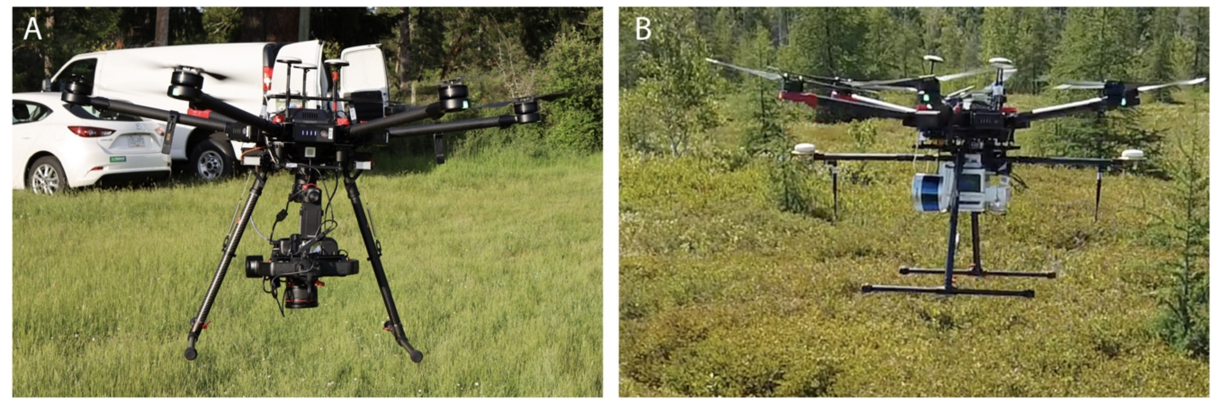
The final SfM and LiDAR point clouds covering 1.71 ha are shown in Figure 3. The SfM dataset has 30,413,182 points while the LiDAR dataset has 1,010,278 points (Table 2). As a result, the SfM point cloud is 19.6 times larger (LAS format) than the LiDAR dataset. The data acquisition time was nearly double for the SfM (18 vs. 10 min), and the computation time to generate the 3D point cloud was at least 10 times greater than for the LiDAR dataset. Considering the time needed to process the geotags and prepare the photographs (i.e., convert from CR2 to JPEG and color correct if necessary), the SfM point cloud takes even longer to generate.
The increased detail obtained from the ≈30x more points in the SfM dataset is apparent in Figure 3, resulting in a more realistic reconstruction of the bog. The several “no data” areas in the LiDAR dataset (shown in black) and the linear pattern of point distribution are artefacts from the mechanical laser diodes spinning during acquisition in a system hard mounted on a moving platform (Figure 2b).
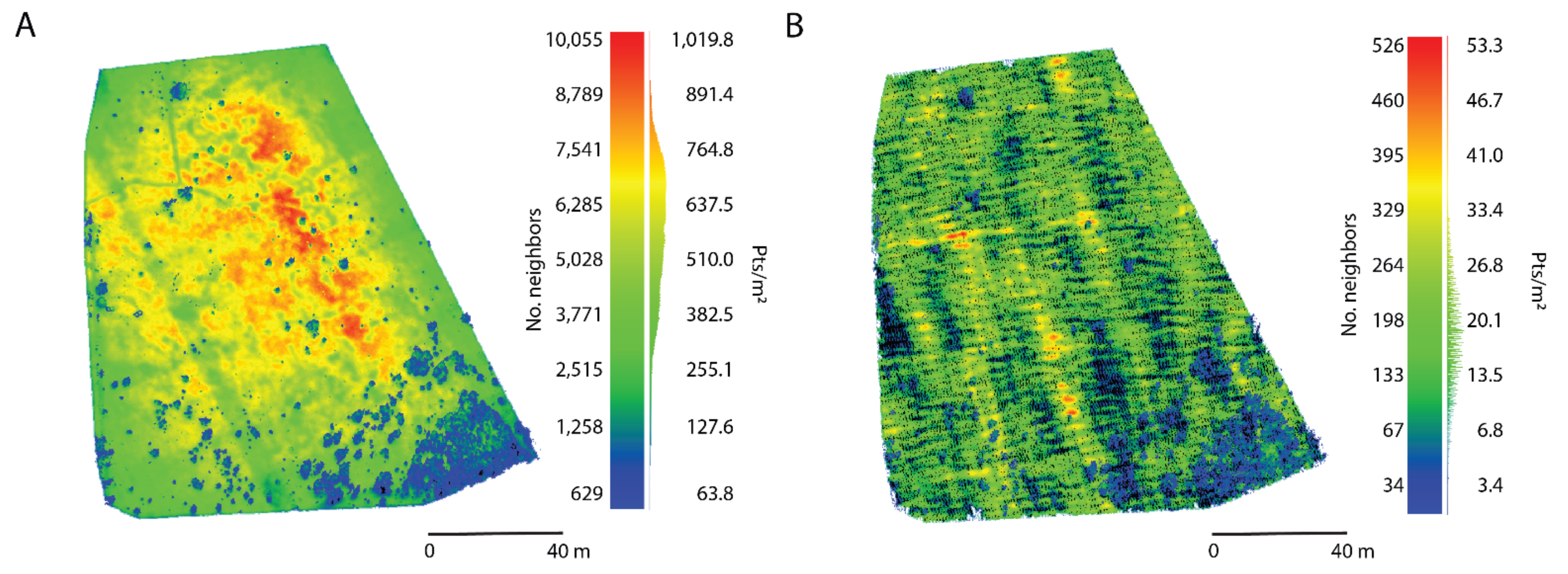
Figure 4 illustrates the point density of the two datasets. The SfM dataset has an average density of 570.4 ± 172.8 pts/m2 while the LiDAR dataset has an average density of 19.4 ± 7.5 pts/m2. In both data sets, the lowest density is in the treed bog.
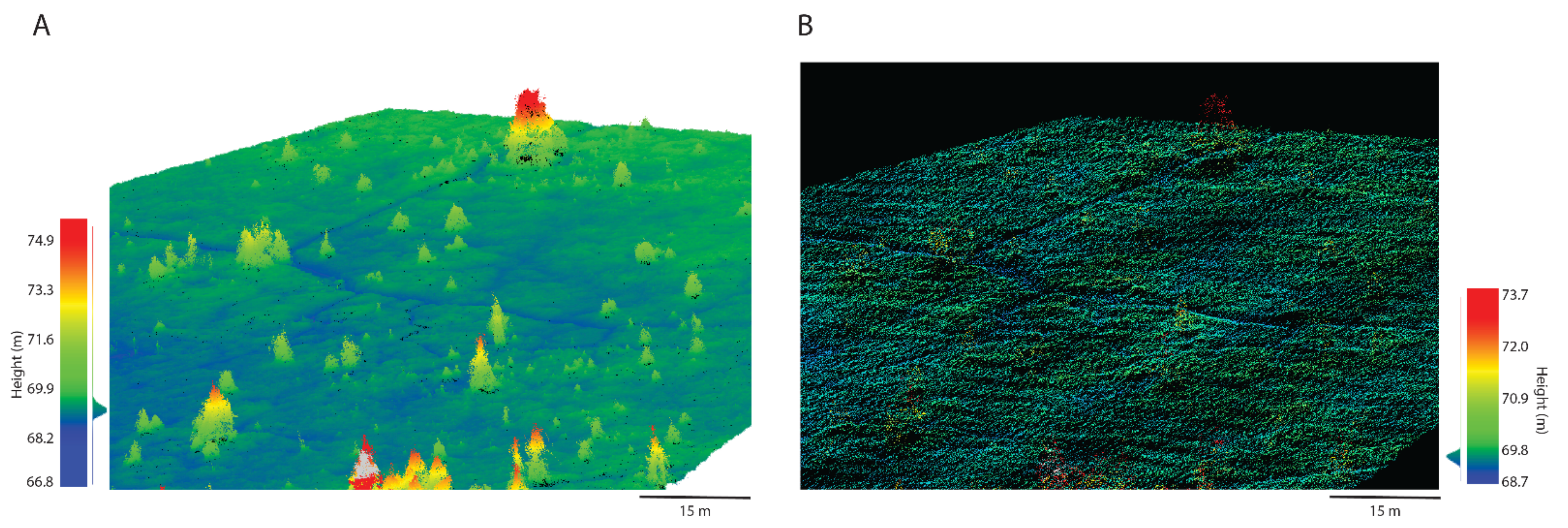
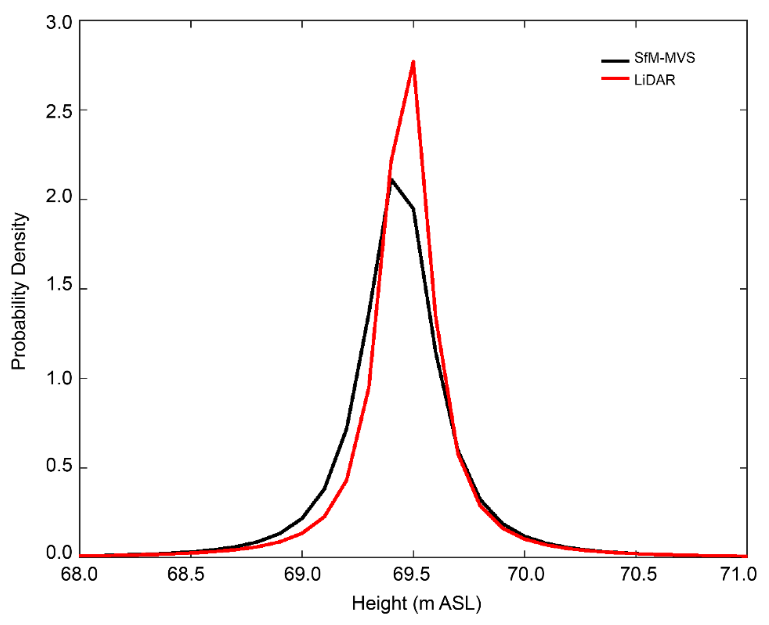
Despite the differences in point density, the gross microtopography and presence of both large and small trees can be seen in both datasets (Figure 5). A t location-scale distribution was found to best fit the vegetation height from both datasets based on the AIC criterion (Table 3, Figure 6). This distribution better represents data with a heavier tail (i.e., more outliers) than a Gaussian one. In this case, relatively fewer points representing the trees are the outliers. The distribution is described by three parameters, location (µ), scale (σ) and shape (ν). Larger values of ν indicate a lesser tail and, therefore, a distribution more similar to a Gaussian. A two-sample Kolmogorov–Smirnov test indicates the height values are from different continuous distributions (k = 0.11, p = 0, α = 0.05). Figure 6 shows that the SfM’s distribution is slightly wider (σ = 1.591) than that of the LiDAR (σ = 0.1151).
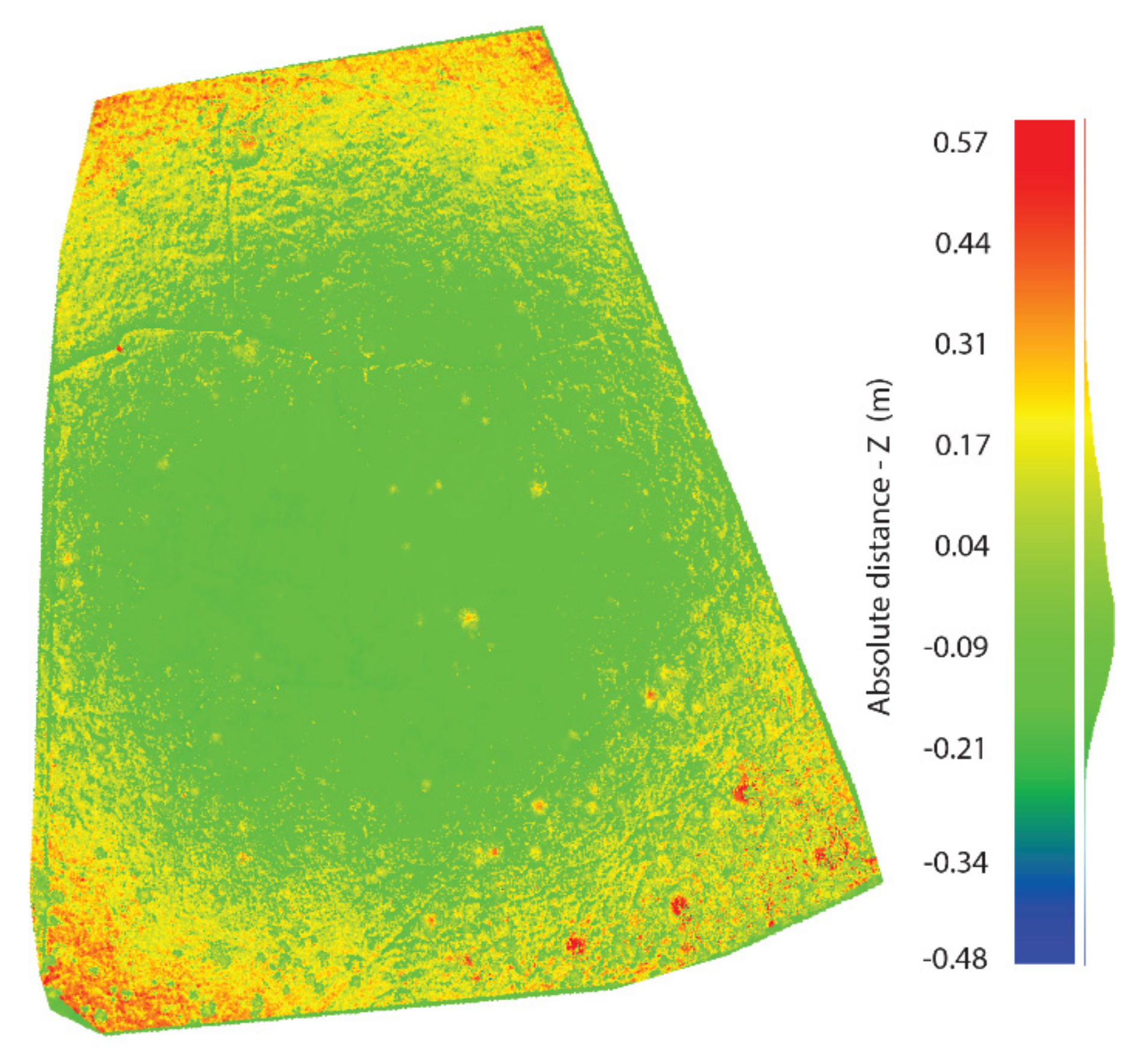
Prior to alignment in CloudCompare, there was a 15 ± 22 cm vertical and 50 ± 7 cm horizontal offset between the point clouds. After ICP, the horizontal offset decreased to 10.5 ± 11.5 cm. The sparseness of the LiDAR point cloud precluded a closer horizontal alignment. Vertically, the difference in height varies by spatial location (average of 4 ± 13 cm) (Figure 7) due to a more pronounced depression in center of the SfM-MVS dataset where the bog has a higher density of hollows. However, when the uncertainties of the height values of both the SfM and LiDAR surfaces are taken into account, the height differences are minimal for the majority of the study area.
The values of surface roughness (Figure 8) reveal similarities across both datasets, with the trees and boardwalks differentiated from the hummocks and hollows with higher values of roughness. In the SfM dataset, hummocks (roughness ≈ 0.1–0.35) can be better differentiated from hollows (roughness ≈ 0.06). From the LiDAR dataset, the sparseness of the point cloud results in incomplete definition of the hummocks (roughness ≈ 0.05–0.29).
After rasterization, the density of the points averaged per pixel of the 10 cm DSM was 17.6 ± 7.3 pts/px from the SfM and 0.6 ± 1.1 pts/px from the LiDAR. At a 50 cm pixel size, the density increased to 437.5 ± 144.4 pts/px for the SfM and 14.5 ± 8.3 pts/px for the LiDAR. The low point density for the LiDAR at the 10 cm pixel size resulted in interpolation artefacts. From the DSMs, the percentages of classified hummocks and hollows are similar between the SfM and LiDAR classifications (Table 4). In both cases, the proportions of the two microforms decreased with increasing pixel size, most notably for the SfM hummock class (loss of 5%). For both pixel sizes, the estimated total area of hummocks and hollows is lower from the LiDAR DSM than those generated from the SfM.
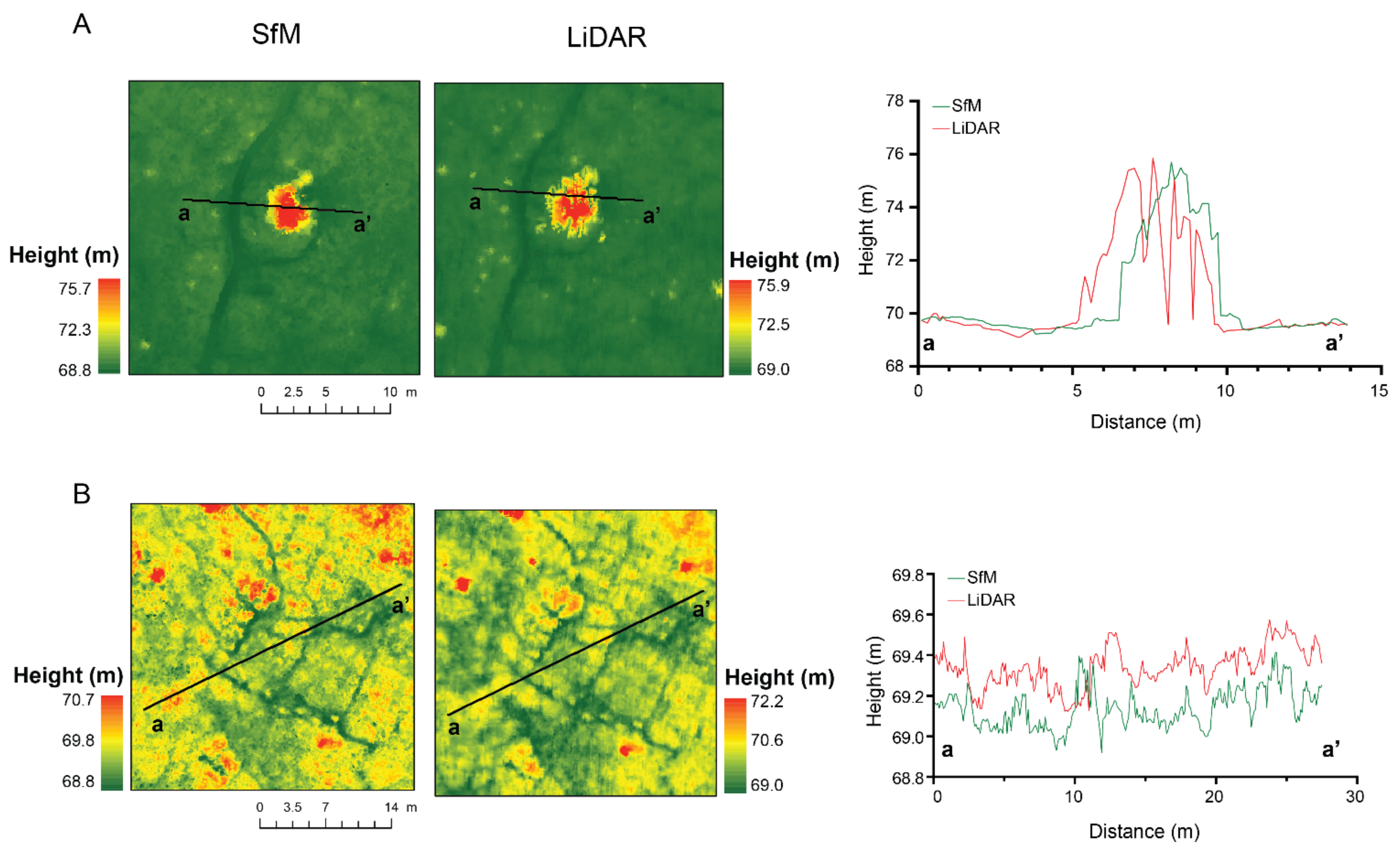
Comparisons of transects (Figure 9) across the profile of a tree and hummocks and hollows, from the 10 cm DSM of each dataset, reveal similarities in the heights along the transects. The remaining horizontal offset between the two datasets is most apparent in the profile of the tree (Figure 9a), but it can also be seen in the hummocks and hollows (Figure 9b) to a lesser degree. The incomplete resolution of the tree crown can be seen in the transect across the tree with sections dropping to ground level due to the low density of the LiDAR. At the finer resolution of the height in the hummocks and hollows transect, a vertical offset of 10–20 cm can be seen between the SfM and LiDAR data. This transect is located near the center of the study area and as can be seen in Figure 7, the difference in height between the datasets in that section is 9–21 cm.
The 3D fractal dimension reveals opposite patterns of complexity between the 10 and 50 cm scales for the SfM and LiDAR derived triangular meshes (Table 5). At both scales, the LiDAR data have higher values of D, indicating greater complexity of the 3D shape of the bog surface. However, this is likely influenced by the sparseness of the point cloud resulting in artefacts following interpolation producing artificial complexity. The lowest value of D (1.36), obtained for the 10 cm SfM data, indicates that at that scale, the microtopography of the bog is more regular. At 50 cm, some of the lawns (height values spanning ±5 cm around the median) that are intermediate between the hummocks and the hollows are grouped together with either the neighboring hummock or hollow, resulting in a more distinct boundary between microforms and a more irregular pattern and greater value of D (1.81).
Similar to the findings of [27], we also found that the bog has an isotropic (nondirectional) semivariogram (from both SfM and LiDAR). From the SfM, the range was approximately 2.5 m with a sill of 0.06 and a nugget of 0.01. The LiDAR had similar results with a range of approximately 2.7 m, a sill of 0.05, and a nugget of 0.01. The semivariograms from both datasets support a hummock–hollow pattern. The longer range value of the LiDAR indicates it was able to resolve a less well-defined pattern between the hummocks and hollows than the SfM.
Lastly, based on the system implementations and acquisition of the data, Table 6 summarizes the main strengths and weaknesses of SfM and LiDAR data acquisition for 3D surface reconstruction of the bog.
3.4. Web-Based Visualization
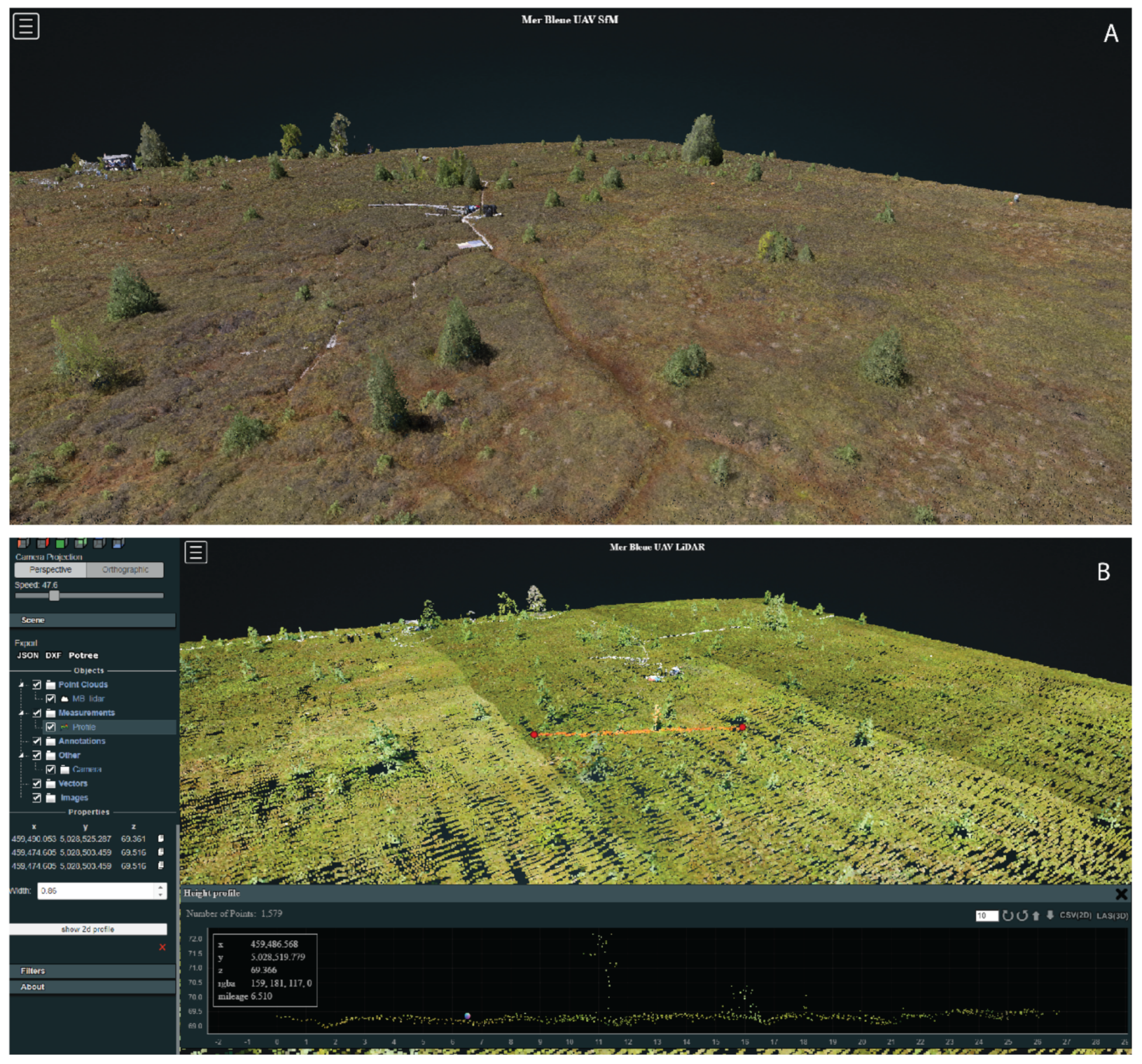
Both point clouds could be visualized in full spatial extent through a web browser from both a desktop computer (Figure 10) and smartphone. Navigation was simple and intuitive using either the mouse (desktop) or by swiping across the screen (smartphone). For both datasets, virtually no lag was experienced when interacting with the point clouds. The basic tools, which included measuring distances and areas and drawing cross sections (Figure 10b), further allowed the user to explore the characteristics of the bog. While interactivity and usability were high, this baseline implementation lacked the “sense being present” within the data. The overall definition of the detail in the point clouds depended on the speed of the internet connection. The server used Cat6 Ethernet to a gigabit broadband connection. From the user side, slow connections, especially on a mobile browser (e.g., HSPA-3G 3.5–14 Mbps), resulted in the point clouds requiring more time to load at full resolution especially for the SfM model (i.e., tens of seconds). On an LTE mobile internet connection (197 Mbps), there was no difference in the speed the models would load (i.e., <5 s) in comparison to a high-speed Wi-Fi or Ethernet connection (i.e., 150–800 Mbps). This web-based implementation is the simplest to access, requiring the user only to click a URL.
3.5. Virtual Reality Visualization
3.5.1. Oculus Quest 2
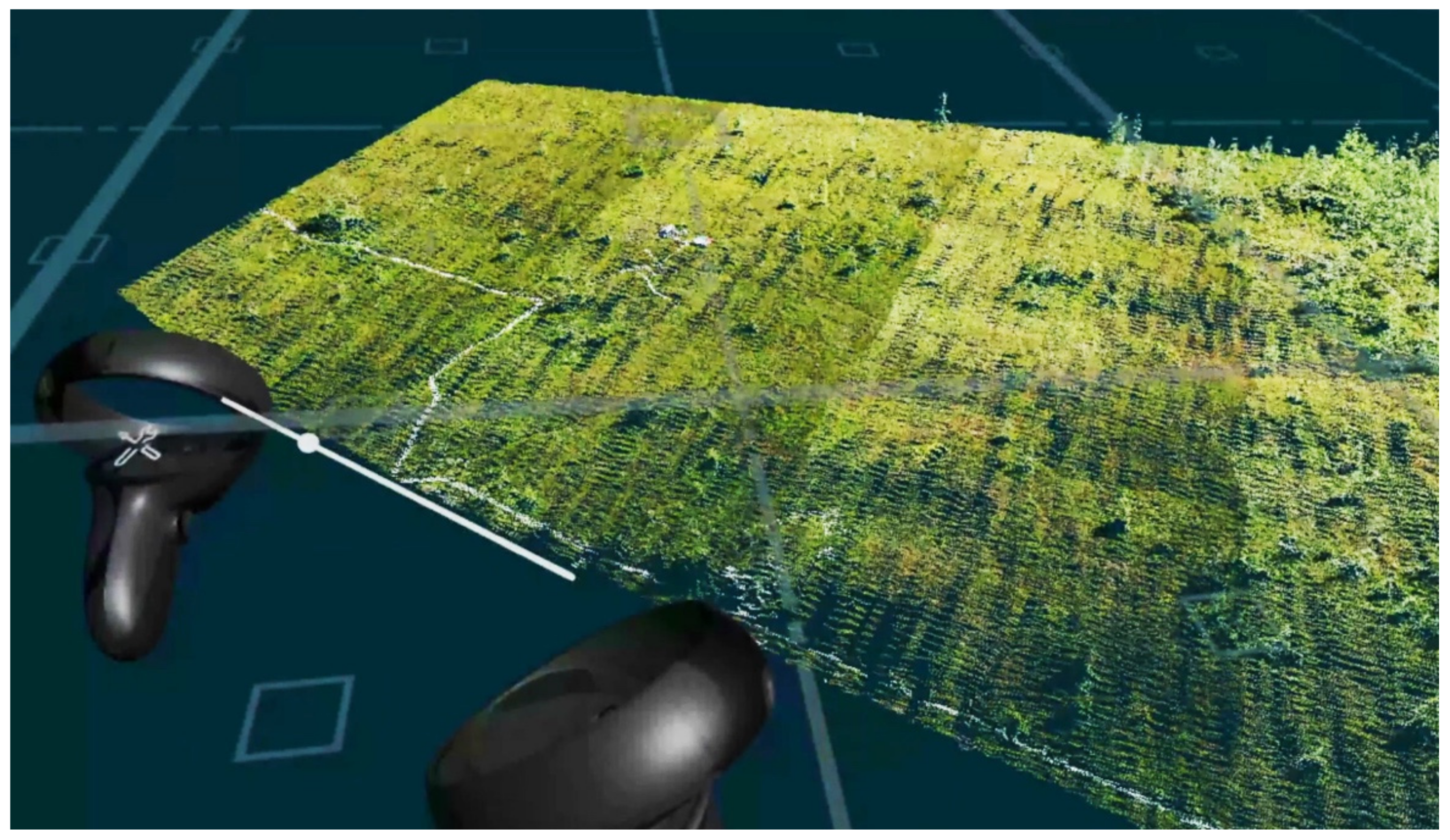
Similar to the web-based visualization, the full point clouds could be loaded and displayed in the HMD through VRifier (Figure 11). The LiDAR point cloud loaded near instantaneously while ≈15–20 s were needed for the SfM model to load. The Oculus Quest 2 provided a full immersive experience with a higher “sense of being present” in the data than what was achieved by the web-based visualization. In this VR implementation, the importance of point density was apparent. With the SfM model, the user has the “next best” experience to being in the bog in person due to the high level of detail while the low point density of the LiDAR resulted in a less realistic experience because of the gaps in the data. Similar to the web-based viewer, the ability to scale the model easily with the touch controllers enhanced the immersive experience.
While generation of the PLY files was straightforward, the setup and integration of the Oculus Quest 2 and the desktop PC were more complicated, requiring the installation and configuration of several software packages and drivers. As of April 2021, VRifier was still in development, and not all features had been implemented. While it was possible to navigate through the point cloud and capture 2D and 3D panoramas (Figure 12) from within VRifier, tools to measure distances or areas were not available. When combined, the software packages (i.e., VRifier, Steam, various Oculus services) committed between 1.5–3 GB of the PC’s RAM and 2.5–3% of the CPU during the visualization of the models.
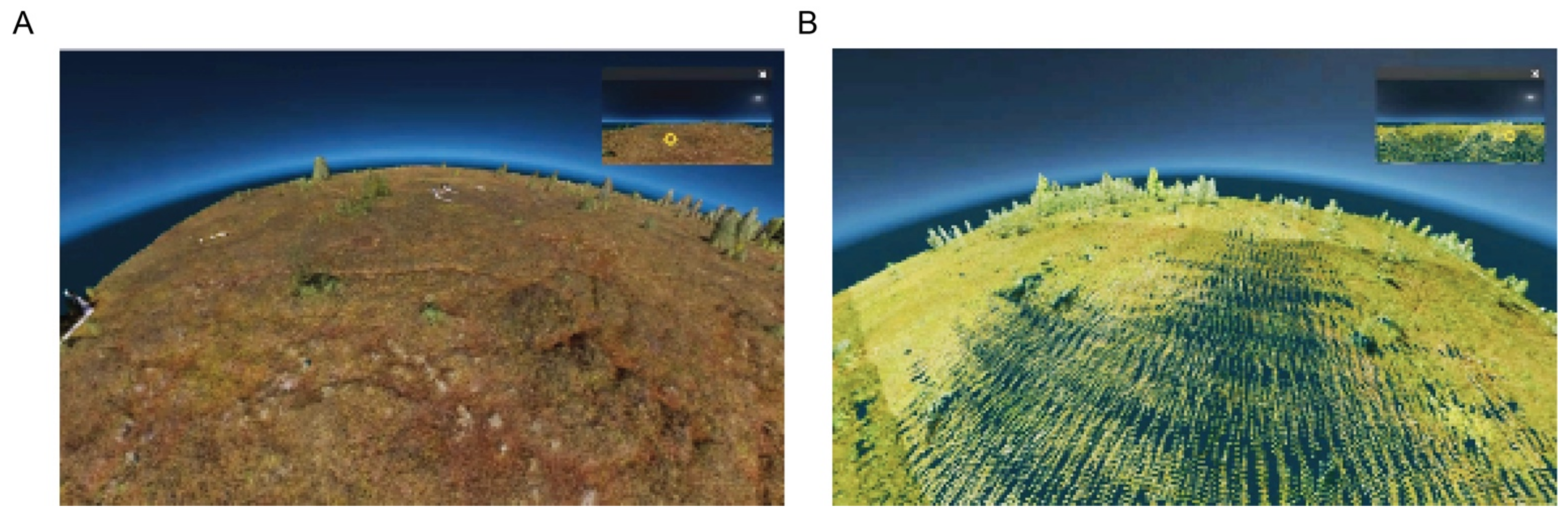
One of the most useful options from within VRifier was the generation of the 360° panoramas (Figure 12). These files (PNG format, .png) can be readily shared, and many free programs are available to view them in 360° format. While they do not provide the navigation element of the immersive experience, these files are a suitable alternative for sharing geospatial data visualization.
3.5.2. Google Cardboard
Other than the web-browser, the Google Cardboard headsets wwere the easiest for visualizing the 3D models. However, the quality of the stereoscopic 3D effect depended on smartphone model used due to the differences in screen size. For example, it was not possible to avoid duplication artefacts with the iPhone XR (screen size 6.06″) with either viewer, but on the iPhone 11 Pro (screen size 5.85″), both viewers worked well in showing clear 3D content. Both viewers are intended to work with screens 4–6″ in size. With the Google 87002823-01 Cardboard viewer, navigation through teleportation within the model was straightforward, but it did not work with the DSCVR headset, in which the experience was more similar to viewing a static 360° 3D photograph. Despite the 3D effect, it was less immersive than with the Oculus Quest 2 implementation.
3.6. Augmented Reality Visualization
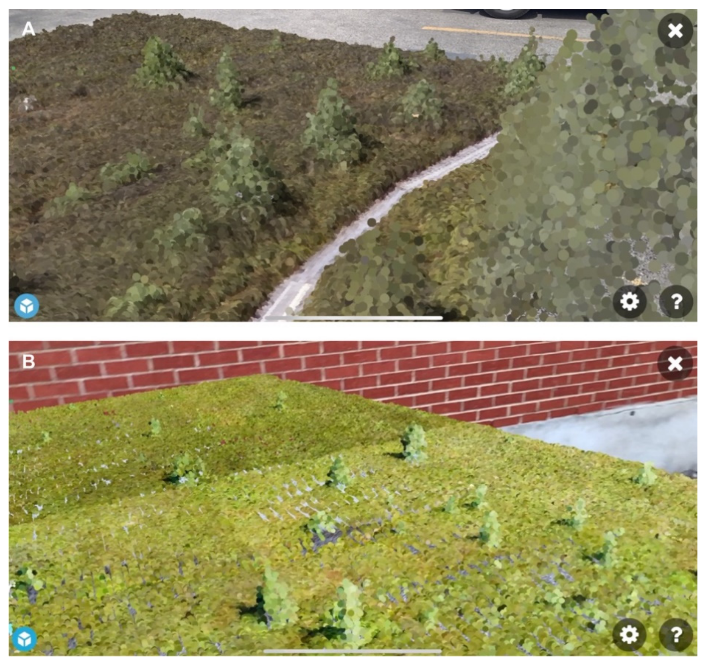
We found the density of the 3D point clouds and the resultant file sizes to be a limiting factor in the usability of the mobile AR viewer. While the entire LiDAR point cloud (14 MB in .ply) could be opened in the Sketchfab application (Figure 13a), the SfM model had to be reduced in overall extent to 788 m2 (20 MB in .ply) (Figure 13b). In addition, the relatively small screen size of the smartphones did not allow for fine scale investigation of the models. Nevertheless, the ability to “walk through” and inspect the models from different viewpoints by simply rotating the phone allowed for a partially immersive experience. With the LiDAR data, the sparseness of the point cloud resulted in the user being able to see through the model to the real-world ground below (Figure 13b), and the hummock–hollow microtopography was very difficult to discern. From the SfM model, gross microtopographic features could be seen on the screen, but because of the small spatial extent of the subset dataset, very little of the bog’s spatial structure could be examined. Table 7 summarizes a comparison between the main considerations of the different point cloud visualizations in VR and AR tested here for the SfM and LiDAR point clouds.
4. Discussion
Microtopography and vegetation patterns at various scales can provide important information about the composition and environmental gradients (e.g., moisture and aeration) in peatlands. Ecological functions, greenhouse gas sequestration, and emission and hydrology can further be inferred from detailed analyses of the vegetation patterns [27,43]. As expected, our study revealed differences between SfM and LiDAR bog microtopography characterizations. The greatest difference is the spatial detail defining the microforms in the point clouds or DSMs. This is a result of the varying point densities, i.e., 570.4 ± 172.8 pts/m2 from the SfM versus 19.4 ± 7.5 pts/m2 from the LiDAR. Despite being sparser than the SfM, the UAS LiDAR data are considerably higher in density than conventional airborne LiDAR data from manned aircraft due to the low altitude of the UAS data collection. For example, airborne LiDAR data over the same study area produced a point cloud with a density of 2–4 pts/m2 [59]. Similarly, the authors in [64] reported a point density of 1–2 pts/m2 from airborne LiDAR for wetlands in Eastern Canada. Nevertheless, the point density achieved here for the LiDAR is lower than that reported by other UAS systems used to study forested ecosystems (e.g., up to 35 pts/m2 [65]).
Contrary to most forest ecosystems with a solid mineral soil ground layer, the ground layer of the bog is composed of living Sphagnum sp. moss over a thick peat column (several meters) with high water content, which prevents the pulses from encountering a solid non-vegetated surface below. Furthermore, the shrubs that comprise the hummocks have a complex branch architecture. A laser pulse encountering vegetation is likely to undergo foliage structural interference, resulting in reduced amplitude of return in comparison to solid open ground [66]. Luscombe et al. (2015) [67] showed that dense bog vegetation disrupts the return of the laser pulses and can result in an uncertain representation of the microform topography. Similar to the authors in [22,25] who found that penetration of the laser pulses into hummock shrub canopy was low from airborne LiDAR, because the vegetation blocked the pulse interaction with the ground beneath hummocks, our results also did not show multiple returns over the hummocks. As can be seen in the cross section of the LiDAR point cloud (Figure 9b), the points follow the elevation of the top of the canopy. A similar phenomenon was noted in other ecosystems with short dense vegetation such as crops and grasslands [27]. The SfM also cannot distinguish between the tops of the hummocks and the moss ground layer beneath. Our results were also similar to those by the authors [23,24] who found that exposed Sphagnum sp. mosses are good planar reflectors for LiDAR, which allows for mapping the surface details in open bogs.
As input to models that require a DSM as part of the workflow or as a covariate, e.g., peat burn intensity mapping [68], biomass estimation [59], and peat depth estimation [21], either the SfM or LiDAR would be sufficient. Both retain the gross microtopography of the bog, with similar semivariogram ranges and complexity (at the 50 cm scale). LiDAR should be used with caution at fine scales of interpolation due to the artefacts introduced from the low point density. Where fine scale detail is required (<10 cm), the SfM provides better results.
While both technologies provide valuable datasets of the bog, they are optimized for different scenarios (Table 6). The SfM dataset is better suited for studies that require fine spatial detail over a smaller area (<10 ha). The longer time for data acquisition and processing make this technology more feasible for localized studies. In contrast, the more efficient LiDAR is better suited to acquiring data over larger areas at lower spatial detail. At the expense of total area covered, from a lower altitude and with a slower flight speed the point density of the LiDAR could be increased, but further testing is required to determine by how much in this ecosystem. Both payloads are of moderate weight, 4.5 kg for the SfM and 4.8 kg for the LiDAR (Table 6) and as such require a UAS with enough payload capacity (e.g., M600P used in our study).
When manipulating the point clouds on a desktop PC or viewing them through the web-based Potree viewer, the difference in file size (1 GB for the SfM vs. 51 MB for the LiDAR LAS files) is not apparent when navigating within or interacting with the dataset. Even with a slow mobile internet connection, the Potree viewer remained useable. The file size also was not an important consideration when viewing the point clouds in VR with the Oculus Quest 2. Because the HMD is tethered to the PC during this operation and the desktop computer is rendering the data, the full datasets can be readily interacted with. When mobile VR (e.g., Google Cardboard) or mobile AR was used, the file size of the SfM dataset hindered the user experience. The main limitation for mobile VR was the file size of the cloud-based hosting platform (i.e., Sketchfab) and RAM capacity of the smartphones for AR. Potentially, the commercial AR implementations developed for medical imaging would not have the same file size restrictions, although these were not tested here.
All VR and AR visualizations provided a sense of agency through the user’s ability to turn their head or smartphone and explore the bog through a full 360° panorama and change their perspective or scale of observation. While this ability is also true for the 360° panoramas captured within VRifer, dynamic agency was only fully achieved by motion tracking in the VR and AR implementations. As described by [69], this is an important distinction between a desktop digital experience and immersive technology. Such transformative developments in visualization lead to the user becoming “part of” the digital representation as opposed to the digital content remaining distinct from the user’s experience [69]. Of the VR and AR tested here, only the Oculus Quest 2 rendered a visually immersive experience. In comparison to other VR implementations such as CAVEs and video walls with smart glasses, the full 360° panoramic view of the VR HMD cannot be matched [70].
Visualization technology is important because it allows users to study areas of interest in virtual environments in 3D, and it facilitates the interaction of groups in different locations, the collection of data in time and space, and the ability to view the object studied in environments with varying scales. In addition to its use in scientific queries, the immersive digital content is a further benefit for educational material and for the individual exploration of questions related to the datasets. Adding virtual models of the region of interest accessible with immersive VR or AR technology greatly benefits the overall understanding and interest in the subject matter [71,72]. Because VR/AR content is interactive, the datasets can now be manipulated by each person with different questions or interests.
With the popularization of this technology for gaming and entertainment, there has been both a surge in development and improvement in the quality of the hardware but also a decrease in price in consumer grade VR headsets. Therefore, it is becoming more feasible to equip teams to use this technology both for meetings and also for virtual collaboration to work with datasets and colleagues from anywhere in the world. Popular for virtual tech support, AR lags behind VR in technological maturity for geospatial visualization. Nevertheless, with more compact datasets, such as the LiDAR point cloud, these 3D scenes can be displayed from most modern smartphones, making it both easily accessible and readily available to share interactive files. With the majority of VR and AR development in fields other than geospatial sciences (e.g., gaming, marketing, telepresence), there is a need for improved functionality and the ability of the specialized software to effectively handle the large files produced from technologies such as SfM and LiDAR [73].
Despite their promise, neither VR nor AR can replicate virtual environments with sufficient detail or fidelity to be indistinguishable from the real world. They are not a substitute for fieldwork, nor firsthand in situ field experiences. Rather, they are tools to augment and enhance geospatial visualization, data exploration, and collaboration.
5. Conclusions
It is only a matter of time before peatland ecosystem models (e.g., [74,75,76]) become adapted for 3D spatially explicit input. Fine-scale microtopographic ecohydrological structures that can be represented from either UAS SfM or LiDAR would provide the resolution needed for models to quantify how peatland structure and function changes over time [67], which can lead to insights into the ecohydrological feedbacks [43]. We show that vegetation structure can be reliably mapped from UAS platforms using either SfM or LiDAR. This is important in sites such as Mer Bleue where the spatial structure of the peatland accounts for 20–40% of the vegetation community distribution [43] and associated ecohydrology. Given the scarcity of UAS LiDAR studies in peatlands (compared to the SfM literature), additional research in peatlands (and other wetlands) is essential. New relatively low-cost LiDAR technologies, such as the DJI’s Zenmuse L1 (point rate of 240,000 pts/s, up to 3 returns and manufacturer stated high vertical and horizontal accuracy), could provide new opportunities to expand the use of LiDAR in peatlands and other ecosystems.
Author Contributions
Conceptualization, M.K. and O.L.; Data curation, M.K.; Formal analysis, M.K. and J.P.A.-M.; Investigation, O.L.; Methodology, M.K.; Writing—original draft, M.K., J.P.A.-M and O.L.; Writing—review & editing, M.K., J.P.A.-M and O.L. All authors have read and agreed to the published version of the manuscript.
Funding
This research was funded by the Canadian Airborne Biodiversity Observatory (CABO) and the Natural Sciences and Engineering Research Council Canada. The APC was funded by MDPI.
Data Availability Statement
The data presented in this study (LAS files) are available on request from the corresponding author following the CABO data use agreement from https://cabo.geog.mcgill.ca (accessed on 14 April 2021).
Acknowledgments
We thank Jacky Heshi from CanDrone for technical support with the LiAIR S220. We also thank the three anonymous reviewers, Nicolas Cadieux, Kathryn Elmer, Deep Inamdar, and Raymond J. Soffer for their comments which helped improved the manuscript.
Conflicts of Interest
The authors declare no conflict of interest. The funders had no role in the design of the study; in the collection, analyses, or interpretation of data; in the writing of the manuscript, or in the decision to publish the results.
Appendix A

Table A1.
Summary of equipment and software used in this study.
| Category | Model | Purpose |
|---|---|---|
| UAS airframe | DJI Matrice 600 Pro | Data acquisition platform |
| RGB camera | Canon 5D Mark III | SfM photograph acquisition |
| Camera gimbal | DJI Ronin MX | SfM photograph acquisition |
| GNSS receiver | Emlid M+ | Geotagging SfM photographs |
| GNSS receiver | Emlid RS+ | Check point acquisition |
| LiDAR | LiAIR S220 | LiDAR data acquisition |
| VR HMD | Oculus Quest 2 | VR visualization |
| AR/VR viewer | iPhone XR, 11 Pro, 12 Pro, Samsung Galaxy 20 FE | Mobile AR visualization |
| VR viewer | Google Official 87002823-01 Cardboard | VR visualization |
| VR viewer | I am Cardboard DSCVR | VR visualization |
| Software | Pix4D | SfM-MVS photogrammetry |
| Software | RTKLib * | SfM geotag PPK |
| Software | LiAcquire | LiDAR acquisition |
| Software | LiNAV | LiDAR postprocessing |
| Software | LiDAR360 | LiDAR postprocessing |
| Software | CloudCompare Stereo * | Point cloud processing/analysis |
| Software | MATLAB | Analysis |
| Software | ProcessOBJ * | Analysis |
| Software | Potree Converter * | Preprocessing point clouds for web-based visualization |
| Software | Potree Server * | Mobile and PC 3D visualization |
| Software | VRifier * | VR visualization |
| Web-based AR/VR viewer | Sketchfab 1,2 | Mobile AR visualization |
1 There is a free plan for individuals with limitations to file size uploaded. 2 Free for users to view models. Open source and free software are designated with an asterisk (*).
References
- Leifeld, J.; Menichetti, L. The underappreciated potential of peatlands in global climate change mitigation strategies. Nat. Commun. 2018, 9, 1071. [Google Scholar] [CrossRef] [PubMed] [Green Version]
- Tarnocai, C.; Kettles, I.M.; Lacelle, B. Peatlands of Canada Database; Research Branch, Agriculture and Agri-Food: Ottawa, ON, Canada, 2005. [Google Scholar]
- Tanneberger, F.; Tegetmeyer, C.; Busse, S.; Barthelmes, A.; Shumka, S.; Moles Mariné, A.; Jenderedjian, K.; Steiner, G.M.; Essl, F.; Etzold, J.; et al. The peatland map of Europe. Mires Peat 2017, 19, 1–17. [Google Scholar]
- Minasny, B.; Berglund, Ö.; Connolly, J.; Hedley, C.; de Vries, F.; Gimona, A.; Kempen, B.; Kidd, D.; Lilja, H.; Malone, B.; et al. Digital mapping of peatlands—A critical review. Earth Sci. Rev. 2019, 196, 102870. [Google Scholar] [CrossRef]
- Poulin, M.F.; Careau, D.; Rochefort, L.; Desrochers, A. From Satellite Imagery to Peatland Vegetation Diversity: How Reliable Are Habitat Maps? Ecol. Soc. 2002, 6, 16. [Google Scholar] [CrossRef] [Green Version]
- Sonnentag, O.; Chen, J.M.; Roberts, D.A.; Talbot, J.; Halligan, K.Q.; Govind, A. Mapping tree and shrub leaf area indices in an ombrotrophic peatland through multiple endmember spectral unmixing. Remote Sens. Environ. 2007, 109, 342–360. [Google Scholar] [CrossRef]
- Kalacska, M.; Arroyo-Mora, J.P.; Soffer, R.J.; Roulet, N.T.; Moore, T.R.; Humphreys, E.; Leblanc, G.; Lucanus, O.; Inamdar, D. Estimating Peatland Water Table Depth and Net Ecosystem Exchange: A Comparison between Satellite and Airborne Imagery. Remote Sens. 2018, 10, 687. [Google Scholar] [CrossRef] [Green Version]
- Kalacska, M.; Lalonde, M.; Moore, T.R. Estimation of foliar chlorophyll and nitrogen content in an ombrotrophic bog from hyperspectral data: Scaling from leaf to image. Remote Sens. Environ. 2015, 169, 270–279. [Google Scholar] [CrossRef]
- Arroyo-Mora, J.P.; Kalacska, M.; Soffer, R.; Ifimov, G.; Leblanc, G.; Schaaf, E.S.; Lucanus, O. Evaluation of phenospectral dynamics with Sentinel-2A using a bottom-up approach in a northern ombrotrophic peatland. Remote Sens. Environ. 2018, 216, 544–560. [Google Scholar] [CrossRef]
- Arroyo-Mora, J.P.; Kalacska, M.; Inamdar, D.; Soffer, R.; Lucanus, O.; Gorman, J.; Naprstek, T.; Schaaf, E.S.; Ifimov, G.; Elmer, K.; et al. Implementation of a UAV–Hyperspectral Pushbroom Imager for Ecological Monitoring. Drones 2019, 3, 12. [Google Scholar] [CrossRef] [Green Version]
- Girard, A.; Schweiger, A.K.; Carteron, A.; Kalacska, M.; Laliberté, E. Foliar Spectra and Traits of Bog Plants across Nitrogen Deposition Gradients. Remote Sens. 2020, 12, 2448. [Google Scholar] [CrossRef]
- Belyea, L.R.; Clymo, R.S. Feedback control of the rate of peat formation. Proc. R. Soc. Lond. Ser. B: Biol. Sci. 2001, 268, 1315–1321. [Google Scholar] [CrossRef] [Green Version]
- Eppinga, M.B.; Rietkerk, M.; Borren, W.; Lapshina, E.D.; Bleuten, W.; Wassen, M.J. Regular Surface Patterning of Peatlands: Confronting Theory with Field Data. Ecosystems 2008, 11, 520–536. [Google Scholar] [CrossRef] [Green Version]
- Nouwakpo, S.K.; Weltz, M.A.; McGwire, K. Assessing the performance of structure-from-motion photogrammetry and terrestrial LiDAR for reconstructing soil surface microtopography of naturally vegetated plots. Earth Surf. Process. Landf. 2016, 41, 308–322. [Google Scholar] [CrossRef]
- Kalacska, M.; Chmura, G.L.; Lucanus, O.; Bérubé, D.; Arroyo-Mora, J.P. Structure from motion will revolutionize analyses of tidal wetland landscapes. Remote Sens. Environ. 2017, 199, 14–24. [Google Scholar] [CrossRef]
- Lovitt, J.; Rahman, M.M.; McDermid, G.J. Assessing the Value of UAV Photogrammetry for Characterizing Terrain in Complex Peatlands. Remote Sens. 2017, 9, 715. [Google Scholar] [CrossRef] [Green Version]
- Dubayah, R.O.; Drake, J.B. Lidar Remote Sensing for Forestry. J. For. 2000, 98, 44–46. [Google Scholar] [CrossRef]
- Ullman, S. The Interpretation of Structure from Motion. Proc. R. Soc. Lond. Ser. B Biol. Sci. 1979, 203, 405–426. [Google Scholar] [CrossRef]
- Westoby, M.J.; Brasington, J.; Glasser, N.F.; Hambrey, M.J.; Reynolds, J.M. ‘Structure-from-Motion’ photogrammetry: A low-cost, effective tool for geoscience applications. Geomorphology 2012, 179, 300–314. [Google Scholar] [CrossRef] [Green Version]
- Iglhaut, J.; Cabo, C.; Puliti, S.; Piermattei, L.; O’Connor, J.; Rosette, J. Structure from Motion Photogrammetry in Forestry: A Review. Curr. For. Rep. 2019, 5, 155–168. [Google Scholar] [CrossRef] [Green Version]
- Gatis, N.; Luscombe, D.J.; Carless, D.; Parry, L.E.; Fyfe, R.M.; Harrod, T.R.; Brazier, R.E.; Anderson, K. Mapping upland peat depth using airborne radiometric and lidar survey data. Geoderma 2019, 335, 78–87. [Google Scholar] [CrossRef]
- Hopkinson, C.; Chasmer, L.E.; Sass, G.; Creed, I.F.; Sitar, M.; Kalbfleisch, W.; Treitz, P. Vegetation class dependent errors in lidar ground elevation and canopy height estimates in a boreal wetland environment. Can. J. Remote Sens. 2014, 31, 191–206. [Google Scholar] [CrossRef]
- Korpela, I.; Haapanen, R.; Korrensalo, A.; Tuittila, E.-S.; Vesala, T. Fine-resolution mapping of microforms of a boreal bog using aerial images and waveform-recording LiDAR. Mires Peat 2020, 26, 1–24. [Google Scholar] [CrossRef]
- Korpela, I.; Koskinen, M.; Vasander, H.; Holopainen, M.; Minkkinen, K. Airborne small-footprint discrete-return LiDAR data in the assessment of boreal mire surface patterns, vegetation, and habitats. For. Ecol. Manag. 2009, 258, 1549–1566. [Google Scholar] [CrossRef]
- Richardson, M.C.; Mitchell, C.P.J.; Branfireun, B.A.; Kolka, R.K. Analysis of airborne LiDAR surveys to quantify the characteristic morphologies of northern forested wetlands. J. Geophys. Res. 2010, 115, 115. [Google Scholar] [CrossRef] [Green Version]
- Langlois, M.N.; Richardson, M.C.; Price, J.S. Delineation of peatland lagg boundaries from airborne LiDAR. J. Geophys. Res. Biogeosci. 2017, 122, 2191–2205. [Google Scholar] [CrossRef]
- Anderson, K.; Bennie, J.; Wetherelt, A. Laser scanning of fine scale pattern along a hydrological gradient in a peatland ecosystem. Landsc. Ecol. 2009, 25, 477–492. [Google Scholar] [CrossRef]
- Gigante, M.A. 1—Virtual Reality: Definitions, History and Applications. In Virtual Reality Systems; Earnshaw, R.A., Gigante, M.A., Jones, H., Eds.; Academic Press: Cambridge, MA, USA, 1993; pp. 3–14. [Google Scholar]
- Le Mouélic, S.; Enguehard, P.; Schmitt, H.H.; Caravaca, G.; Seignovert, B.; Mangold, N.; Combe, J.-P.; Civet, F. Investigating Lunar Boulders at the Apollo 17 Landing Site Using Photogrammetry and Virtual Reality. Remote Sens. 2020, 12, 1900. [Google Scholar] [CrossRef]
- Li, L.; Yu, F.; Shi, D.; Shi, J.; Tian, Z.; Yang, J.; Wang, X.; Jiang, Q. Application of virtual reality technology in clinical medicine. Am. J. Transl. Res. 2017, 9, 3867–3880. [Google Scholar]
- Leigh, C.; Heron, G.; Wilson, E.; Gregory, T.; Clifford, S.; Holloway, J.; McBain, M.; Gonzalez, F.; McGree, J.; Brown, R.; et al. Using virtual reality and thermal imagery to improve statistical modelling of vulnerable and protected species. PLoS ONE 2019, 14, e0217809. [Google Scholar] [CrossRef] [Green Version]
- Ching-Rong, L.; Loffin, R.B.; Stark, T. Virtual reality for geosciences visualization. In Proceedings of the 3rd Asia Pacific Computer Human Interaction (Cat. No.98EX110), Shoan Village Center, Kangawa, Japan, 15–17 July 1998; pp. 196–201. [Google Scholar]
- Billen, M.I.; Kreylos, O.; Hamann, B.; Jadamec, M.A.; Kellogg, L.H.; Staadt, O.; Sumner, D.Y. A geoscience perspective on immersive 3D gridded data visualization. Comput. Geosci. 2008, 34, 1056–1072. [Google Scholar] [CrossRef] [Green Version]
- Berger, H.; Dittenbach, M.; Merkl, D.; Bogdanovych, A.; Simoff, S.; Sierra, C. Opening new dimensions for e-Tourism. Virtual Real. 2006, 11, 75–87. [Google Scholar] [CrossRef] [Green Version]
- Bruno, F.; Barbieri, L.; Lagudi, A.; Cozza, M.; Cozza, A.; Peluso, R.; Muzzupappa, M. Virtual dives into the underwater archaeological treasures of South Italy. Virtual Real. 2017, 22, 91–102. [Google Scholar] [CrossRef]
- Chang, Y.-L.; Tien, C.-L. Development of mobile augmented-reality and virtual-reality simulated training systems for marine ecology education. In Proceedings of the 24th International Conference on 3D Web Technology, Los Angeles, CA, USA, 26–28 July 2019; pp. 1–3. [Google Scholar]
- Huang, J.; Lucash, M.S.; Scheller, R.M.; Klippel, A. Walking through the forests of the future: Using data-driven virtual reality to visualize forests under climate change. Int. J. Geogr. Inf. Sci. 2020, 10, 1–24. [Google Scholar] [CrossRef]
- Liberatore, M.J.; Wagner, W.P. Virtual, mixed, and augmented reality: A systematic review for immersive systems research. Virtual Real. 2021. [Google Scholar] [CrossRef]
- Scavarelli, A.; Arya, A.; Teather, R.J. Virtual reality and augmented reality in social learning spaces: A literature review. Virtual Real. 2020, 25, 257–277. [Google Scholar] [CrossRef]
- Lafleur, P.M.; Hember, R.A.; Admiral, S.W.; Roulet, N.T. Annual and seasonal variability in evapotranspiration and water table at a shrub-covered bog in southern Ontario, Canada. Hydrol. Process. 2005, 19, 3533–3550. [Google Scholar] [CrossRef]
- Bubier, J.L.; Moore, T.R.; Crosby, G. Fine-scale vegetation distribution in a cool temperate peatland. Can. J. Bot. 2006, 84, 910–923. [Google Scholar] [CrossRef]
- Lafleur, P.M.; Roulet, N.T.; Bubier, J.L.; Frolking, S.; Moore, T.R. Interannual variability in the peatland-atmosphere carbon dioxide exchange at an ombrotrophic bog. Glob. Biogeochem. Cycles 2003, 17, 13. [Google Scholar] [CrossRef] [Green Version]
- Malhotra, A.; Roulet, N.T.; Wilson, P.; Giroux-Bougard, X.; Harris, L.I. Ecohydrological feedbacks in peatlands: An empirical test of the relationship among vegetation, microtopography and water table. Ecohydrology 2016, 9, 1346–1357. [Google Scholar] [CrossRef]
- Hassel, K.; Kyrkjeeide, M.O.; Yousefi, N.; Prestø, T.; Stenøien, H.K.; Shaw, J.A.; Flatberg, K.I. Sphagnum divinum (sp. nov.) and S. medium Limpr. and their relationship to S. magellanicum Brid. J. Bryol. 2018, 40, 197–222. [Google Scholar] [CrossRef]
- Moore, T.R.; Bubier, J.L.; Frolking, S.E.; Lafleur, P.M.; Roulet, N.T. Plant biomass and production and CO2 exchange in an ombrotrophic bog. J. Ecol. 2002, 90, 25–36. [Google Scholar] [CrossRef]
- Arroyo-Mora, J.; Kalacska, M.; Soffer, R.; Moore, T.; Roulet, N.; Juutinen, S.; Ifimov, G.; Leblanc, G.; Inamdar, D. Airborne Hyperspectral Evaluation of Maximum Gross Photosynthesis, Gravimetric Water Content, and CO2 Uptake Efficiency of the Mer Bleue Ombrotrophic Peatland. Remote Sens. 2018, 10, 565. [Google Scholar] [CrossRef] [Green Version]
- DJI. D-RTK User Manual; DJI: Schenzen, China, 2017. [Google Scholar]
- Lucanus, O.; Kalacska, M. UAV DSLR Photogrammetry with PPK Processing. Available online: https://www.protocols.io/view/uav-dslr-photogrammetry-with-ppk-processing-bjm2kk8e (accessed on 30 March 2020).
- Natural Resources Canada. Station Report. Available online: https://webapp.geod.nrcan.gc.ca/geod/data-donnees/station/report-rapport.php?id=943020 (accessed on 1 March 2021).
- Takasu, T.; Yasuda, A. Development of the low-cost RTK-GPS receiver with an open source program package RTKLIB. In Proceedings of the International Symposium on GPS/GNSS, Jeju, Korea, 11 April 2009; pp. 4–6. [Google Scholar]
- Pix4D. Initial Processing > Calibration. Available online: https://support.pix4d.com/hc/en-us/articles/205327965-Menu-Process-Processing-Options-1-Initial-Processing-Calibration (accessed on 1 March 2021).
- Strecha, C.; Kung, O.; Fua, P. Automatic mapping from ultra-light UAV imagery. In Proceedings of the 2012 European Calibration and Orientation Workshop, Barcelona, Spain, 8–10 February 2012; pp. 1–4. [Google Scholar]
- Strecha, C.; Bronstein, A.; Bronstein, M.M.; Fua, P. LDAHash: Improved Matching with Smaller Descriptors. IEEE Trans. Pattern Anal. Mach. Intell. 2012, 34, 66–78. [Google Scholar] [CrossRef] [Green Version]
- Strecha, C.; von Hansen, W.; Van Gool, L.; Fua, P.; Thoennessen, U. On Benchmarking camera calibration and multi-view stereo for high resolution imagery. In Proceedings of the IEEE Conference on Computer Vision and Pattern Recognition, Anchorage, AK, USA, 23–28 June 2008. [Google Scholar]
- Kalacska, M.; Lucanus, O.; Arroyo-Mora, J.P.; Laliberté, É.; Elmer, K.; Leblanc, G.; Groves, A. Accuracy of 3D Landscape Reconstruction without Ground Control Points Using Different UAS Platforms. Drones 2020, 4, 13. [Google Scholar] [CrossRef] [Green Version]
- GreenValley Interantional. LiAir 220 UAV 3D Mapping System. Available online: https://www.greenvalleyintl.com/wp-content/uploads/2019/09/LiAir220.pdf (accessed on 1 March 2021).
- Hesai. Pandar40P 40-Channel Mechanical LiDAR. Available online: https://www.hesaitech.com/en/Pandar40P (accessed on 10 March 2021).
- Hesai. Pandar40P 40-Channel Mechanical LiDAR User Manual; Hesai: Shanghai, China; p. 74.
- Inamdar, D.; Kalacska, M.; Arroyo-Mora, J.; Leblanc, G. The Directly-Georeferenced Hyperspectral Point Cloud (DHPC): Preserving the Integrity of Hyperspectral Imaging Data. Front. Remote Sens. Data Fusion Assim. 2021, 2, 675323. [Google Scholar] [CrossRef]
- Backes, A.R.; Eler, D.M.; Minghim, R.; Bruno, O.M. Characterizing 3D shapes using fractal dimension. In Progress in Pattern Recognition, Image Analysis, Computer Vision, and Applications SE-7; Bloch, I., Cesar, R., Jr., Eds.; Springer: Berlin/Heidelberg, Germany, 2012; pp. 14–21. [Google Scholar]
- Reichert, J.; Backes, A.R.; Schubert, P.; Wilke, T.; Mahon, A. The power of 3D fractal dimensions for comparative shape and structural complexity analyses of irregularly shaped organisms. Methods Ecol. Evol. 2017, 8, 1650–1658. [Google Scholar] [CrossRef]
- Halley, J.M.; Hartley, S.; Kallimanis, A.S.; Kunin, W.E.; Lennon, J.J.; Sgardelis, S.P. Uses and abuses of fractal methodology in ecology. Ecol. Lett. 2004, 7, 254–271. [Google Scholar] [CrossRef]
- Schuetz, M. Potree: Rendering Large Point Clouds in Web Browsers; Vienna University of Technology: Vienna, Austria, 2016. [Google Scholar]
- LaRocque, A.; Phiri, C.; Leblon, B.; Pirotti, F.; Connor, K.; Hanson, A. Wetland Mapping with Landsat 8 OLI, Sentinel-1, ALOS-1 PALSAR, and LiDAR Data in Southern New Brunswick, Canada. Remote Sens. 2020, 12, 2095. [Google Scholar] [CrossRef]
- Davenport, I.J.; McNicol, I.; Mitchard, E.T.A.; Dargie, G.; Suspense, I.; Milongo, B.; Bocko, Y.E.; Hawthorne, D.; Lawson, I.; Baird, A.J.; et al. First Evidence of Peat Domes in the Congo Basin using LiDAR from a Fixed-Wing Drone. Remote Sens. 2020, 12, 2196. [Google Scholar] [CrossRef]
- Garroway, K.; Hopkinson, C.; Jamieson, R. Surface moisture and vegetation influences on lidar intensity data in an agricultural watershed. Can. J. Remote Sens. 2014, 37, 275–284. [Google Scholar] [CrossRef]
- Luscombe, D.J.; Anderson, K.; Gatis, N.; Wetherelt, A.; Grand-Clement, E.; Brazier, R.E. What does airborne LiDAR really measure in upland ecosystems? Ecohydrology 2015, 8, 584–594. [Google Scholar] [CrossRef] [Green Version]
- Chasmer, L.E.; Hopkinson, C.D.; Petrone, R.M.; Sitar, M. Using Multitemporal and Multispectral Airborne Lidar to Assess Depth of Peat Loss and Correspondence With a New Active Normalized Burn Ratio for Wildfires. Geophys. Res. Lett. 2017, 44, 11851–11859. [Google Scholar] [CrossRef] [Green Version]
- Klippel, A.; Zhao, J.; Oprean, D.; Wallgrün, J.O.; Stubbs, C.; La Femina, P.; Jackson, K.L. The value of being there: Toward a science of immersive virtual field trips. Virtual Real. 2019, 24, 753–770. [Google Scholar] [CrossRef]
- Cerfontaine, P.A.; Mreyen, A.-S.; Havenith, H.-B. Immersive visualization of geophysical data. In Proceedings of the 2016 International Conference on 3D Imaging, Liege, Belgium, 13–14 December 2008. [Google Scholar]
- Karanth, S.; Murthy S., R. Augmented Reality in Visual Learning. In ICT Analysis and Applications; Springer: Singapore, 2021; pp. 223–233. [Google Scholar]
- Raiyn, J. The Role of Visual Learning in Improving Students’ High-Order Thinking Skills. J. Educ. Pract. 2016, 7, 115–121. [Google Scholar]
- Nesbit, P.R.; Boulding, A.; Hugenholtz, C.; Durkin, P.; Hubbard, S. Visualization and Sharing of 3D Digital Outcrop Models to Promote Open Science. GSA Today 2020, 30, 4–10. [Google Scholar] [CrossRef] [Green Version]
- Frolking, S.; Talbot, J.; Jones, M.C.; Treat, C.C.; Kauffman, J.B.; Tuittila, E.-S.; Roulet, N. Peatlands in the Earth’s 21st century climate system. Environ. Rev. 2011, 19, 371–396. [Google Scholar] [CrossRef]
- Wu, J.; Roulet, N.T.; Moore, T.R.; Lafleur, P.; Humphreys, E. Dealing with microtopography of an ombrotrophic bog for simulating ecosystem-level CO2 exchanges. Ecol. Model. 2011, 222, 1038–1047. [Google Scholar] [CrossRef]
- Gong, J.; Roulet, N.; Frolking, S.; Peltola, H.; Laine, A.M.; Kokkonen, N.; Tuittila, E.-S. Modelling the habitat preference of two key Sphagnum species in a poor fen as controlled by capitulum water content. Biogeosciences 2020, 17, 5693–5719. [Google Scholar] [CrossRef]
Figure 1.
(A) Map of Mer Bleue, near Ottawa in Ontario, Canada. Locations where photographs B–E were taken are indicated on the map. (B) UAV photograph facing north, taken in October; (C) photograph facing SE across the study area, taken in June; (D) UAV photograph of the southern margin of the study area where dense stands of Typha latifolia (cattail) grow in areas of permanent slow-moving water impacted by beavers. Photograph facing west, taken in May. (E) Photograph facing the treed bog, taken in June. A 360° aerial panorama acquired in late June can be viewed at https://bit.ly/mbpano2017 (accessed on 14 April 2021).


Figure 2.
M600P RTK enabled UAV with the (A) Canon DSLR and (B) LiAIR S220.

Figure 3.
The final 1.71 ha point clouds for the bog study area from (A) SfM and (B) LiDAR at three increasing levels of scale.
Figure 3.
The final 1.71 ha point clouds for the bog study area from (A) SfM and (B) LiDAR at three increasing levels of scale.

Figure 4.
Point density of the (A) SfM and (B) LiDAR datasets. The number of neighbors is the count of points within a sphere with a 1 m radius. The pts/m2 represents the number of points within a surface area of 1 m2. The distribution next to the color bars represents the histogram of the height values. No data shown in black.

Figure 5.
Subset of the point clouds illustrating the height of the vegetation (m ASL) for a subset of the point cloud from (A) SfM and (B) LiDAR. The distribution next to the color bars represents the histogram of the height values.
Figure 5.
Subset of the point clouds illustrating the height of the vegetation (m ASL) for a subset of the point cloud from (A) SfM and (B) LiDAR. The distribution next to the color bars represents the histogram of the height values.

Figure 6.
Best-fit t location-scale distribution probability density functions of height for the SfM and LiDAR datasets.
Figure 6.
Best-fit t location-scale distribution probability density functions of height for the SfM and LiDAR datasets.

Figure 7.
Difference in height between the SfM and LiDAR point clouds. The distribution next to the color bar represents the histogram of the difference in height.
Figure 7.
Difference in height between the SfM and LiDAR point clouds. The distribution next to the color bar represents the histogram of the difference in height.

Figure 8.
Surface roughness for (A) SfM and (B) LiDAR datasets calculated with a kernel size of 1 m (the radius a sphere centered on each point). The distributions next to the color bars represent the histogram of the roughness values.
Figure 8.
Surface roughness for (A) SfM and (B) LiDAR datasets calculated with a kernel size of 1 m (the radius a sphere centered on each point). The distributions next to the color bars represent the histogram of the roughness values.

Figure 9.
Comparison of transects across a profile of a tree (A) and hummocks and hollows (B) for the SfM and LiDAR datasets. The panels on the left illustrate the DSMs from which the transects were extracted.
Figure 9.
Comparison of transects across a profile of a tree (A) and hummocks and hollows (B) for the SfM and LiDAR datasets. The panels on the left illustrate the DSMs from which the transects were extracted.

Figure 10.
Screen captures illustrating the (A) SfM and (B) LiDAR point clouds in the web-based Potree viewer. The LiDAR data are shown with the cross-section tool enabled, illustrating that while the microtopography is difficult to see in the point cloud due to the low density of points, when viewed as a cross section, the difference in elevation between the hummocks and hollows is visible. The point clouds can be viewed at https://bit.ly/MB_SfM (accessed on 14 April 2021) and https://bit.ly/MB_lidar (accessed on 14 April 2021), respectively.

Figure 11.
Video from VRifier illustrating the experience navigating the SfM and LiDAR point clouds on the Oculus Quest 2 headset. The input PLY files and video are available for download from https://doi.org/10.5281/zenodo.4692367 (accessed on 14 April 2021).
Figure 11.
Video from VRifier illustrating the experience navigating the SfM and LiDAR point clouds on the Oculus Quest 2 headset. The input PLY files and video are available for download from https://doi.org/10.5281/zenodo.4692367 (accessed on 14 April 2021).

Figure 12.
Videos illustrating 360° panoramas of the (A) SfM and (B) LiDAR point clouds within VRifier. These panoramas are being viewed on the Insta360 Player but can be opened by most 360° photograph viewers. The 360° panoramas are available for download from https://doi.org/10.5281/zenodo.4692367 (accessed on 14 April 2021).

Figure 13.
Videos illustrating a screen recording of the AR visualization of the (A) SfM and (B) LiDAR point clouds through the iOS Sketchfab application. The models can be viewed in AR at https://skfb.ly/onuU9 (LiDAR) (accessed on 14 April 2021) and https://skfb.ly/onuUs (SfM) (accessed on 14 April 2021).

Table 1.
Quality metrics of the full individual LiDAR strips calculated from LiDAR360.
| Quality Metric | Value |
|---|---|
| Overlap between strips (%) | 50.8–52.2 |
| RMSE before boresight correction (cm) | 8.6 |
| RMSE after correction (cm) | 8.4 |
| Elevation difference between strips, RMSEz (HU–HO) (cm) | 5.8–7.1 |
| Elevation difference between strips, RMSEz (trees) (cm) | 13.1–17.3 |
| 1 Average density (pts/m2) | 25.3–31.2 |
| 1 Density range (pts/m2) | 1–270 |
| Trajectory deformation (%) | 0.22–0.55 |
1 These values represent the full strips, including edges without overlap, turns, and infrastructure (sheds) that were cut from the final dataset.
Table 2.
Comparison between the final bog SfM and LiDAR datasets.
| Characteristic | SfM | LiDAR |
|---|---|---|
| Area (ha) | 1.71 | 1.71 |
| Acquisition altitude (m) | 50 | 50 |
| Acquisition speed (m/s) | 2.5 | 5 |
| 1 Total flight time (min) | ≈18 | ≈10 |
| Average Density (pts/ha) | ≈17.7M | ≈0.6M |
| Total number of points | 30,413,182 | 1,010,278 |
| Density as pts/m2 (µ ± σ) | 570.4 ± 172.8 | 19.4 ± 7.5 |
| 2 File size, LAS format (total area in MB) | 1000 | 51 |
| 2 File size, LAS format (MB/ha) | 585 | 30 |
| 2 File size, PLY format (total area in MB) | 445 | 15 |
| 2 File size, PLY format (MB/ha) | 260.2 | 8.8 |
| 3 Computation time (min) | ≈150 | ≈15 |
1 Includes transit from takeoff area and the two sets of figure 8s required for the LiDAR INS calibration after takeoff and before landing, and does not include time on the ground between flights. 2 These files contain only six columns: x, y, z coordinates and R, G, B color intensity. 3 Does not include time needed to covert or geotag the photographs for the SfM.
Table 3.
Parameters of the best-fit t location-scale distributions of height (m ASL) from the two datasets; µ = location, σ = scale, ν = shape, CI = confidence interval.
Table 3.
Parameters of the best-fit t location-scale distributions of height (m ASL) from the two datasets; µ = location, σ = scale, ν = shape, CI = confidence interval.
| Dataset | AIC | µ | σ | ν | CI µ | CI σ | CI ν |
|---|---|---|---|---|---|---|---|
| SfM-MVS | 1.0879 × 10⁷ | 69.436 | 0.1591 | 1.87 | 69.4359–69.4361 | 0.1590–0.1592 | 1.816–1.819 |
| LiDAR | 8.2967 × 10⁴ | 69.470 | 0.1151 | 1.40 | 69.4697–69.4703 | 0.1148–0.1154 | 1.397–1.407 |
Table 4.
Percentage of hummocks (HU) and hollows (HO) in the study area classified from the SfM and LiDAR DSMs.
Table 4.
Percentage of hummocks (HU) and hollows (HO) in the study area classified from the SfM and LiDAR DSMs.
| Pixel Size | SfM HO | SfM HU | LiDAR HO | LiDAR HU |
|---|---|---|---|---|
| 10 cm | 28.8 | 28.6 | 29.9 | 25.6 |
| 50 cm | 27.8 | 23.6 | 22.1 | 24.0 |
Table 5.
Value of the 3D Minkowski–Bouligand fractal dimension (D) for the SfM and LiDAR.
| Pixel Size | SfM | LiDAR |
|---|---|---|
| 10 cm | 1.36 | 1.86 |
| 50 cm | 1.81 | 1.83 |
Table 6.
Comparison of general SfM and LiDAR acquisition strengths and weaknesses.
| Characteristic | SfM | LiDAR |
|---|---|---|
| Acquisition | Slow | Fast |
| System initialization | Starts acquisition after takeoff | Requires INS calibration after takeoff and before landing |
| Line spacing | Narrow (e.g., 15 m @ 50 m AGL with 80% sidelap) | Wide (e.g., 40 m @ 50 m AGL with 50% overlap) |
| Processing time | Slow | Fast |
| Resolution of spatial detail | Ultra-high | Moderate |
| User friendliness | Low–high 1 | High |
| Consistency of results | Moderate–high | High |
| Potential for component failure | Low–high 2 | Low |
| Payload implementation | Easy–difficult 3 | Easy |
| File size | Large | Small |
| Payload weight (kg) | 4.5 | 4.8 |
1 System described here has a low user-friendliness (i.e., complex to operate) but integrated systems (e.g., Phantom 4 RTK [55]) are more user friendly. 2 System described here has a high potential for component failure unlike integrated systems. 3 The DSLR setup described here requires precise balancing of the camera on the gimbal, which can be difficult and time consuming to achieve in the field. This is not a concern for integrated systems.
Table 7.
Qualitative comparison between main considerations for visualization of the LiDAR and SfM point clouds.
Table 7.
Qualitative comparison between main considerations for visualization of the LiDAR and SfM point clouds.
| Characteristic | Web-Based | Oculus Quest 2 VR | Google Cardboard (VR) | Mobile AR |
|---|---|---|---|---|
| Sense of being present | Low | High | Moderate | Low |
| Ease of use | High | Moderate | Moderate–high | High |
| Ease of setup | Moderate | Low | High | High |
| File size supported | Ultra-large | Ultra-large | Moderate | Limited |
| Equipment cost (setup) | High | Moderate | Low | Low |
| Equipment cost (user) | Low/high | Moderate | Low | Low |
| Long-term cost effectiveness | High | High | Low–high | Low |
| Requires internet | Yes/No 1 | No 2 | Yes/No 3 | Yes |
1 A local PC installation of the Potree viewer that does not require access to the internet to view the models is available. 2 After initial setup, internet access is not required. 3 Models could be saved locally to the smartphone and accessed without internet.
Publisher’s Note: MDPI stays neutral with regard to jurisdictional claims in published maps and institutional affiliations. |
© 2021 by the authors. Licensee MDPI, Basel, Switzerland. This article is an open access article distributed under the terms and conditions of the Creative Commons Attribution (CC BY) license (https://creativecommons.org/licenses/by/4.0/).
Share and Cite
MDPI and ACS Style
Kalacska, M.; Arroyo-Mora, J.P.; Lucanus, O. Comparing UAS LiDAR and Structure-from-Motion Photogrammetry for Peatland Mapping and Virtual Reality (VR) Visualization. Drones 2021, 5, 36. https://doi.org/10.3390/drones5020036
AMA Style
Kalacska M, Arroyo-Mora JP, Lucanus O. Comparing UAS LiDAR and Structure-from-Motion Photogrammetry for Peatland Mapping and Virtual Reality (VR) Visualization. Drones. 2021; 5(2):36. https://doi.org/10.3390/drones5020036
Chicago/Turabian StyleKalacska, Margaret, J. Pablo Arroyo-Mora, and Oliver Lucanus. 2021. "Comparing UAS LiDAR and Structure-from-Motion Photogrammetry for Peatland Mapping and Virtual Reality (VR) Visualization" Drones 5, no. 2: 36. https://doi.org/10.3390/drones5020036