
Using Neural Networks for Bicycle Route Planning


Faculty of Electrical Engineering, Mechanical Engineering, and Naval Architecture (FESB), Ruđera Boškovića 32, HR-21000 Split, Croatia
*
Author to whom correspondence should be addressed.
Appl. Sci. 2021, 11(21), 10065; https://doi.org/10.3390/app112110065
Submission received: 16 July 2021
/
Revised: 22 October 2021
/
Accepted: 25 October 2021
/
Published: 27 October 2021
(This article belongs to the Section Computing and Artificial Intelligence)
Abstract
:This paper presents the usage of artificial neural networks (NNs) in bicycle route planning. This research aimed to check the possibility of NNs to transfer human expertise in bicycle route design by training the NN on an already established set of bicycle routes and then using the trained NN to design the routes on the novel area. We created two NNs capable of choosing the best route among the given road network by training them on two different areas. The bicycle routes produced by NNs were the same at best and had 75% overlap at the worst compared to those produced by human experts. Furthermore, the mean square error for all of our NN models varied from 0.015 and 0.081. We compared this new approach to the traditional multicriteria GIS (geographic information system) analysis (MA) that requires the human expert to define the bicycle route selection criteria. The benefit of using NN over the MA was that the NN directly transfers the human expertise to a model. In contrast, the MA needs the expert to select multiple criteria and adjust their weights carefully.
1. Introduction
The promotion of bicycle usage can have various benefits, such as ecological, health, and economic. Encouraging bicycles instead of public transportation and cars is significant for carbon footprint reduction. In addition, to promote bicycle usage, there has to be an infrastructure for a safer and more convenient bicycle ride.
Bicycle usage plays an essential role in the tourist offer of rural areas and the Adriatic Sea islands. These parts of Croatia have vast, remote areas containing many green surfaces, lakes, and forests. Significant for the tourist offer of these areas is the possibility of bicycle usage because such natural environments can be experienced in the best way using a bicycle. To give a good quality bicycle experience in these remote areas, one has to take care of health service coverage. Telemedicine plays a vital role in covering the rural areas with health services [1,2], increasing the safety of a bicycle ride.
NNs are inspired by the performance and structure of the biological neural network [3]. A structure consisting of processing units assembled in an interconnected network is called neural networks (NNs). It is evident that the human possibility for pattern recognition tasks is superior over computers, but there is a possibility to realise some features using NN. New computing models based on NN are explored to solve complex pattern recognition tasks. The NN can adjust connection weights when learning from example patterns.
MA in GIS is a well-established method whereby carefully selecting criteria and adjusting their weights can make a complex analysis. On the other hand, using NNs in GIS is relatively recent. NNs found their usage in real-world complex problem modelling. Its structure consists of many interrelated processing elements. Their ability to perform many parallel computations used in knowledge representation and knowledge presentation is their main advantage [4]. The engagingness of NNs comes from the biological systems processing characteristics, including learning, robustness, high parallelism, fault and failure tolerance, and capability to generalise and handle imprecise and fuzzy information [5]. In this paper, we have trained two NNs on two existing bicycle route networks. First, we evaluated the NNs by using the network trained on one area to create routes for the other area and compared routes created by NN to the base truth—the routes already existing in the other area. After that, we used NNs to create a new network in a different area. When comparing routes created by NN with those created with an MA analysis, we found that NN chose similar routes as MA, which proved that our MA gives sound results.
This research aimed to investigate the possibility of NN to transfer human expertise in bicycle route design by training the NN on an already established set of bicycle routes and then using the trained NN to design the routes on a novel area. We compared this new approach to the traditional MA that requires the human expert to define the bicycle route selection criteria (instead of learning and transferring the expert knowledge in NNs).
In Section 2, the previous work regarding the area studied in this paper is presented. Section 3.1. Describes producing bicycle route models using MA. The other approach using NN for model production is shown in Section 3.2. Two approaches comparison and obtained results are shown in Section 4. The discussion about provided results is presented in Section 5, and the conclusion referring to the results is made in Section 6.
2. Previous Work
The subject of bicycle route planning is beginning to appear in the literature in the past decade. The literature search process started with using the MA, in which we searched for previous usages of MA in route selection and continued with the literature review in NN usage with GIS. Our previous work [6] showed that GIS could be employed in a rural area to produce bicycle routes based on MA analysis. Hsu and Lin presented the bicycle route suitability assessment based on MA [7]. To determine the criteria for the route selection, the authors used the geographic information system and the expert opinion survey employed for each criterion weight calculation, combined with the fuzzy analytic hierarchy process (FAHP). It is a practical tool in criteria determination for imprecise semantics [8,9]. After using FAHP to interpret the expert opinion survey, the acquired results were used as an input for calculating the most suitable route. In this work, ref. [7] Hsu and Lin concluded that GIS usage is helpful for comprehensive model evolvent for bicycle network planning.
Chen, Shen, and Clidress in [10] analysed which criteria cyclists paid the most excellent attention to when choosing their route. As a source of cyclist tracking data, they used the GPS data from the mobile application “Cycletracks” for the Seattle area (WA, USA). One or more factors influenced the selection of a bicycle route. There are three groups in which the factors can be assigned: convenience-related factors (e.g., stopover points, bike racks and lockers availability, trip distance), safety-related factors (e.g., street lighting, speed limits, bicycle facility type) and leisure-related factors (e.g., parks, street trees shading, distance to mountains and water bodies, monumental places of interests). Some factors can relate to all three groups: slope degree, pavement quality, and the number of intersections with signalisation. The GPS data were gleaned for three and a half years [9]. A sum of 4.9 million GPS points was used to produce 3310 routes. The analysis detected safety as an essential bicycle route choice factor. A second important criterion was leisure-related—the cyclist chooses routes located near green areas and water.
Huang and Ye [11] created a process of bicycle routes selection using GIS and applied it to the city of Berkeley. This procedure consisted of creating a database, choosing the most suitable path between each start location-end location pair, and gathering results to pick out the most suitable routes. The criteria authors selected to determine a bicycle route desirability are the travel duration, the road traffic, the slope grade, and the road surface conditions. The travel time included intersection delay and distance; road traffic included air pollution and traffic conflicts. The road surface conditions included the smoothness of the road and its width. This paper concluded that GIS is helpful for bicycle route choice since it can use different available sources and integrate them. GIS is also essential because of its possibility to capture spatial criteria, which is essential to cycling.
An interesting approach is shown in [12], where Bi et al. considered different road users in an urban area. They propose a unifying NN model for time and energy-efficient routes calculations within an urban road network. Authors had ecological motivation since their case study in Beijing showed a reduction of average travel time by 20% and energy consumption by 10%. Interesting usage of NNs and GIS is shown in [13], where the author checks the success rate of NN in predictions of landslides using GIS tools and technologies. The performance of such a network is 71.3% which the author considered as encouraging. In [14], the authors showed a principle in which they used both static and dynamic information in route planning among obstacles originating from a forest fire. In addition, the authors provided an extended A* algorithm for obstacle-avoiding route calculation with consideration to the predicted information apropos roads state, departure time, and speed of vehicles. They concluded that with the usage of the extended algorithm, among dynamic data provided by fire simulations, a safe path to the destination was calculated.
The usage of NNs increased in recent years because of their wide area of application. NNs are increasingly applied in managing transportation infrastructures. In [15], De Luca combined NN with GIS systems for road accident predictions. He compared the results of NN prediction with the multivariate analysis (MVA) and showed that both techniques provided good predictions. Similarly, in the paper [16], Sameen and Pradhan used recurrent neural networks (RNN) to predict the traffic accidents’ seriousness. The RNNs are NNs containing feedback connections designed for sequence modelling. Feedback connections assure the past activation memory, which provides the learning dynamics of sequential data. The authors concluded that the RNN model achieved the best accuracy in traffic accident injury severity. The paper [17] was dealing with an optimisation model for slowing down the congestion in urban traffic; Song and Quan used ArcGIS technology and MATLAB to optimise the bus line around the scope of population distribution. Another exciting application of GIS and NN usage combination is shown by Kia et al. in [18]. A flood model was developed with diverse flooding causative factors using GIS and NN techniques for flood-prone areas simulation. In model training, seven input nodes were used, each representing parameters which cause a flood. They concluded that this model is accurate enough and might provide a significant advantage along with a warning system operating in real-time. Shah et al. [19] combined GIS with ANN for road safety risk analysis; a new methodological approach in road safety risk evaluation is presented. ANN was used to calculate the predictability of risk value, while GIS was used to produce geospatial output. The authors concluded that ANN with GIS provided an efficient and easy output in road safety data analysis and safety improvement decision making. Pritchard, Frøyen and Snizek in [20] presented bicycle level of service (BLOS)–GIS-based indicators to estimate link suitability in transport networks. The authors concluded that the BLOS method could assist in bicycle route generation, but the number of generated unique routes is low.
Grekousis et al. [21] presented the integration of GIS with artificial intelligence for modelling urban evolution. For clusters representing the level of urbanisation level creation, the authors used the fuzzy c-means algorithm. With the usage of the produced clusters, authors could monitor region development from a rural area to an urban area with a large population. The authors registered the final results in a geodatabase and used GIS software to visualise them. NNs were used for urban evolution prediction by observing the changes in the region’s neighbouring area. The network is trained to learn how individual units evolve and what is the influence of these changes on the neighbouring areas. The authors concluded that the combination of GIS, fuzzy logic, and NN with the proposed methodology, along with a complete database, delineates the future urbanism level more reliably.
3. Materials and Methods
3.1. Modelling Bicycle Path Using the Multicriteria Analysis
Based on the paper [10], convenience, safety, and leisure objectives will be considered for bicycle route choice. Convenience is an objective based on choosing the most efficient bicycle route, e.g., the shortest path. The safety objective has a focus on injury risk minimisation. Finally, the leisure objective is related to pleasures acquired from cycling, e.g., places of interest, scenic views.
3.1.1. Points of Interest
The road network of the Croatian town Imotski was used for the route selection model. Since cycling in this area is mainly tourism-oriented, leisure was the model’s most important objective. Therefore, the aim was to create a bicycle route that will link points of interest in the Imotski area. Among all points of interest in Imotski area, nine were chosen: Blue and Red Lake (the most favoured tourist attraction, water-filled massive sinkholes), Dva oka (lake with the shape of two eyes), Prološko blato (Proložac lake), Tin Ujević’s statue (Croatian writer), Perinuša (mill on the Vrljika river), Panoramic view on Proložac lake, Topana (Imotski fortress), Zelena katedrala (Green cathedral).
3.1.2. Criteria Choice
Considering the research [11], the criteria picked for bicycle route desirability determination are:
- Road segment length;
- Road type;
- Slope grade;
- Distance between the Emergency unit and the road segment;
- Distance between the drinking water source and the road segment.
Our road network topology consisted of road segments and nodes. A road segment connects two nodes; it is a part of the road between two road intersections. All five criteria used for a route desirability determination were assigned to a particular road segment.
The length of a road segment was taken as the criteria in the route model, considering the desire to choose the shortest path. That means that the shorter road segment will more likely be chosen as the best one.
Road type was taken as the criterion for bicycle route desirability determination based on safety reasons. Since the road infrastructure in the Imotski area is weak, it is safer for the bicyclist to ride on roads of a higher category because they are kept in a better condition than the lower category roads.
The distance to the emergency unit is also a safety-related criterion. Therefore, the model will produce paths gravitating to emergency units; in case of an accident, the distance to the emergency unit will be minimised.
The length between the source of drinking water and the road segment is primarily a leisure-related criterion, even though it can be partly considered as a safety-related criterion. Since there are many drinkable water sources in the lowland part of the Imotski area, it can be used to provide better security and comfort in riding a bicycle.
ESRI ArcGIS software was used to build the bicycle route model. The primary sources of information were topographic maps in scale 1:25,000 and maps in the scale of 1:5000 collected from the Croatian State geodetic administration.
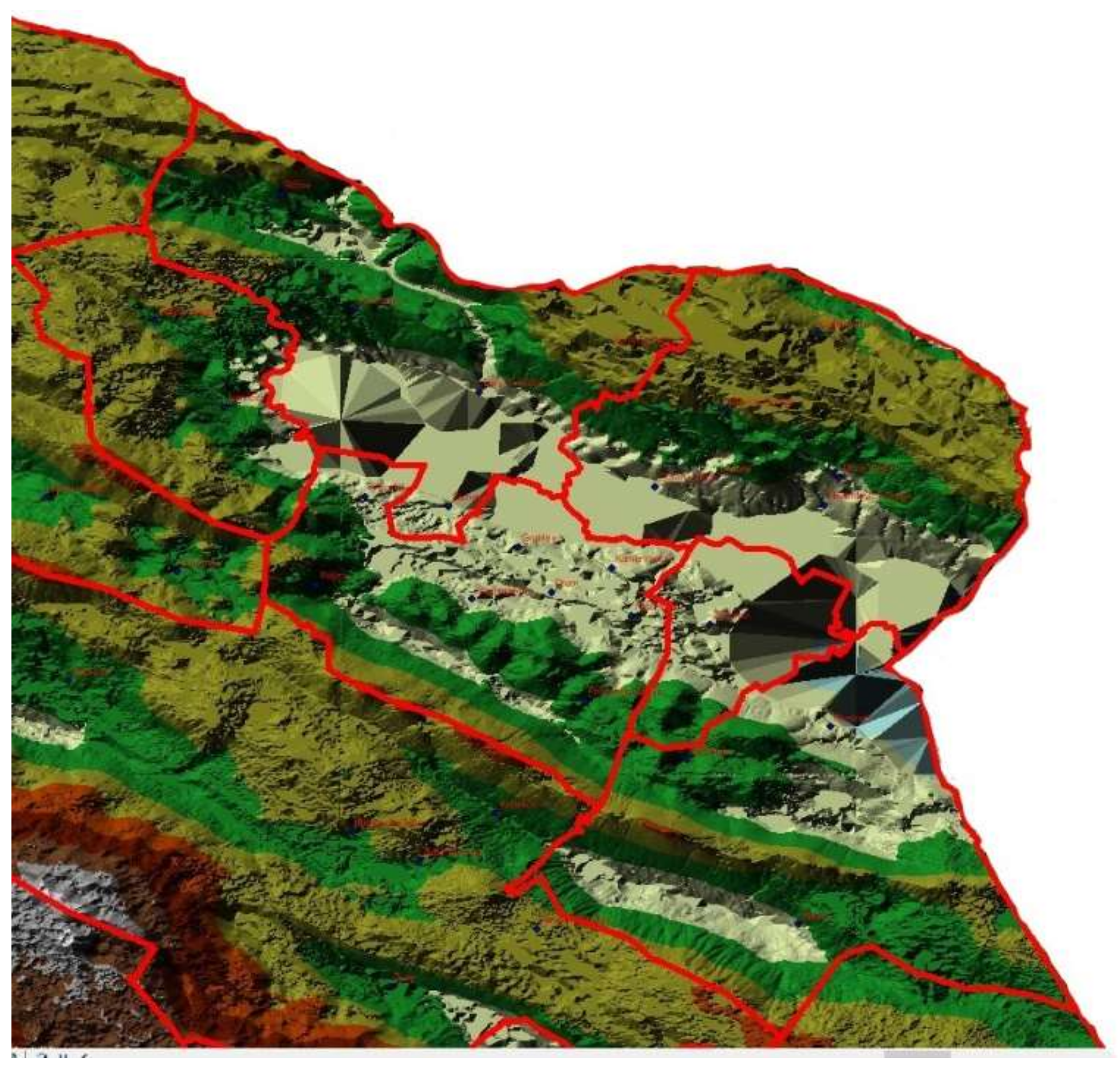
Using the data containing information about the height of the terrain from maps, the relief model of the Imotski area (Figure 1) has been reconstructed.
Triangulated irregular network (TIN) relief model was reconstructed using layers containing height data obtained from a topographic map on a scale of 1:25,000. The height data resolution is 50 m. TIN is vector-based data generated by triangulating vertices connected with a series of edges and then forming a triangle network, with resolution higher in the more dynamic areas.
The TIN model was used to calculate the slope grade, which could have both negative and positive effects on the bicycle path decision. The most professional bicyclist would instead pick bicycle routes that are more challenging, such as longer and steeper routes. Contrarily, some people use a bicycle irregularly, and they do not have enough endurance. Therefore, two different models for each type of bicyclist will be built.
3.1.3. Model Parameters
The network analyst extension was employed to produce the bicycle route model from input data. Input data consist of parameters and stops; stops are places that must be a part of the route. Parameters are criteria that influence the model production by picking the chosen path. First, the network, which consists of Imotski area roads, was produced. After that, we normalised our five criteria for parameters in the following way. The points of interest were included as stops in the GIS. The criteria which were previously chosen were included in the GIS as the parameters. The road type and road length were used from the road attribute data. To incorporate the distance from the emergency unit, we used the extension called the closest facility. It was employed to compute the shortest reach between the emergency unit and every road segment. Before that, it was necessary to create points from polylines that make the road layer. It was decided that one point per road segment is precise enough due to the ratio between mean road segments length and the emergency unit and water source mean distance. The mean length of road segments is 1556.06 m, and the mean distance to the emergency unit and water source is 22,388.26 m. We used the closest facility tool for the shortest distance calculation between every road segment existing in the Imotski area and the water stream segment, which is the closest to the road segment. Before employing the closest facility, we created points from water stream segments polylines.
A relief model was used to acquire slope gradient information for each road segment. To meet that objective, we used the Add Surface Information geoprocessing tool. Input data were TIN, and the output was each road segment’s average slope.
3.1.4. Model Production
For the most appropriate route calculation between two or more places established on the travelling salesman problem [22], the network analyst tool was employed. Since the accuracy of the selected route by the travelling salesman problem was a priority, we decided to use the naive approach in calculating the most appropriate route. In the naive approach (which is a brute-force approach), the first point is considered the starting and ending point, after which the cost of every permutation is calculated while the minimum cost is kept tracked. Considering the number of segments, we could insist on precision and use the brute-force approach.
The criterion data for the model (weights) were normalised [23]. Normalisation was necessary since different criteria had different natures and ranges, so without normalisation, the effect of the individual criteria would not be equal. For example, the mean value for the road segment length is 1406 meters, and for average slope, 5.23%—the road segment unit is a meter, and the average slope is expressed as a road height-length ratio. Therefore, the following equation was used for criteria normalisation:
where Xi presents the ith data in the criteria dataset, Ximin is the minimum value of the observed criterion data, and Ximax is the maximum value of the observed criterion data. After normalising data finished, the value of all weights was between 0 and 1. Road segment weight was calculated by summing each criterion normalised data and input in the network analyst extension; this produced the path aimed at beginner bicyclists, as it preferred flatter slopes. We also created a path for professional cyclists who prefer more challenging routes. We did this by adjusting weights in the model to preferer steeper slopes and longer distances. Three paths this model produced will be presented and discussed in Section 4.
3.2. Modelling Bicycle Paths Using Neural Networks
The other approach to multicriteria road analysis, aiming to find the most suitable path, is using artificial intelligence.
Encouraged by paper [17], we decided to compare the results provided by the ArcGIS Network Analyst tool with the results provided by various NN architectures. For the NN training and testing, the “nntool” from MATLAB was used.
Neural Network Details
Similar to the previous chapters’ GIS modelling described, we used NN to model two bicycle routes: the flatter one and the steeper one. The first step was to train both models. As the source of information for model training, we decided to use the existing bicycle routes. We used web pages [24,25] as the data source for training our NN model. We decided to use bicycle routes from Vrgorac town and Knin area since their similarity with Imotski in location, elevation, and relief.
For Vrgorac town, we used the “Tri polja” route as the training data for the flatter route (it is marked as the semi-flat on the website) and the “Mate Svjetskoga” route as the training data for the steeper route (marked as steep in the website). For the Knin area, as the training data for the flatter route, the “Lopuška glavica” route was used since it was marked as flat on the website. Finally, the steeper route model was built based on the “Napoleonova staza” route marked as steep on the website.
Using these four routes, we trained four models of our NN. The input for NNs were road segments. The number of segments used as input to the NN is shown in Table 1. The input for each segment was the same data as in the MA models—five normalised parameters presented in 3.1.2. There was no weight added to the parameter’s value; input to the NN was normalised parameter’s data. The score for segments used in the route was set to 1, while those not used were set to 0.
The gathering and labelling training data were time-consuming—scores for road segments needed to be labelled manually. However, the training process carried out in MATLAB was fast for the number of layers we were dealing with.
After we trained the four NN models, two for the Knin area and two for the Vrgorac area, we used trained networks on road segments in the Imotski area. The score given by the NN gave us information on which road segment can be considered suitable for a bicycle route. The road segment’s suitability for the bicycle route was expressed as a number ranged [0,1]. The value closer to 0 showed that the NN model decided that the road segment is not desirable, while the value closer to 1 showed that the road segment is desirable.
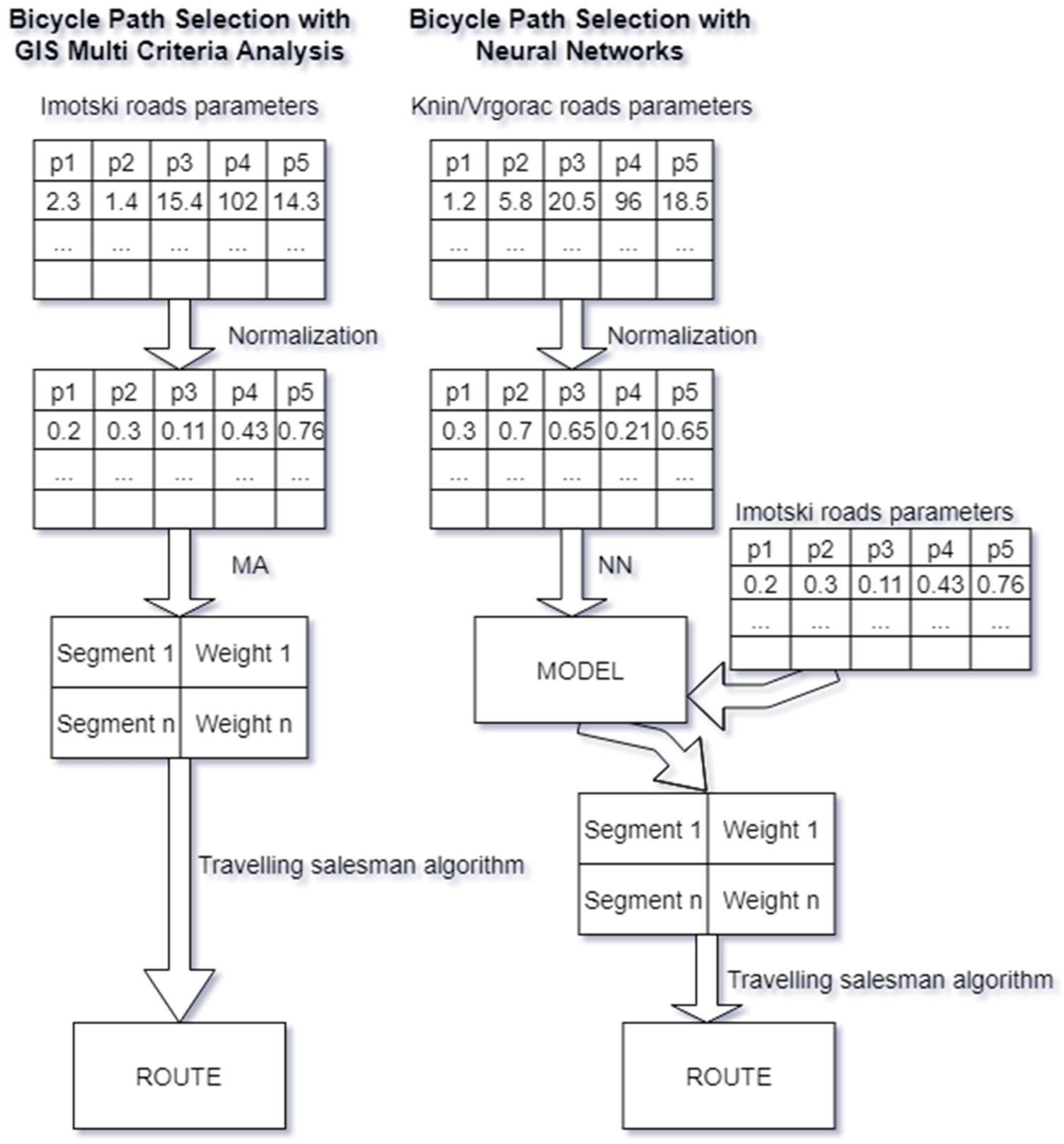
We created a hybrid model that combines the brute force algorithm for the travelling salesman problem with NN to produce the NN routes. As stated before, the NN gave information about each road segment’s desirability expressed by numbers ranged [0,1]. That information was used as a road segment weight, and the travelling salesman problem was used to connect points of interest, but now with the NNs information (Figure 2). On the right side of this figure, one can see the workflow for bicycle path selection using NN compared to the workflow when using GIS MA analysis. The first part of both methods is to determine the weights of road segments. With GIS MA, this is performed using a formula specified by the operator. With NN, the weights are produced by the NN trained on other already established bicycle paths. The second part of both methods is to apply the travelling salesman problem to the network road topology.
Since the roads segment data were arranged so that the connected segment data are located next to each other, we decided to use the layer recurrent NN.
The network architecture was made of five layers. The input layer contained ten neurons, while the output layer has one neuron. In hidden layers, the second layer had one neuron; the rest of the hidden layers consisted of 10 neurons. This NN constitution was chosen due to the compromise between the training speed and accuracy. We noticed that, with the neural number increasing (e.g., a number of learning parameters increase), the training time also increased, but the model’s accuracy has not significantly improved. The Levenberg–Marquardt backpropagation [26] was used as a training function; it uses a Levenberg–Marquardt optimisation for weight and bias weight update. It requires more memory than the other training functions available in nntool, but it is recommended since it is the fastest. The Levenberg–Marquardt algorithm does not use the Hessian matrix, which can be approximated as:
and the gradient can be calculated as:
J is the Jacobian matrix containing network errors first derivatives concerning the weights and biases, while e is a vector of network errors. T stands for transposition, µ is the damping factor that is adjusted at each iteration; it is decreased after each successful step and decreased if that would increase the performance function. I is the identity matrix. The Levenberg–Marquardt algorithm can calculate the Jacobian matrix using the approximation that is much less complex than Hessian matrix computation:
The gradient descent with momentum weight and bias learning function was used in our training process as an adaption learning function. The choice of learning rate has a great impact on NN performance. It is a number that tells how the error is going to affect model weight parameters. Adaptive learning functions can adapt the learning rate for all weights in NN, where momentum will consider the weight delta from the previous iteration to calculate weight in the current iteration. MSE (mean-squared error) was used as a performance function.
In this work, we used hyperbolic tangent sigmoid transfer function as the activation function of each neuron as:
This activation function is bounded and continuous, which makes it compatible with the backprop NN.
Training parameters are shown in Table 2.
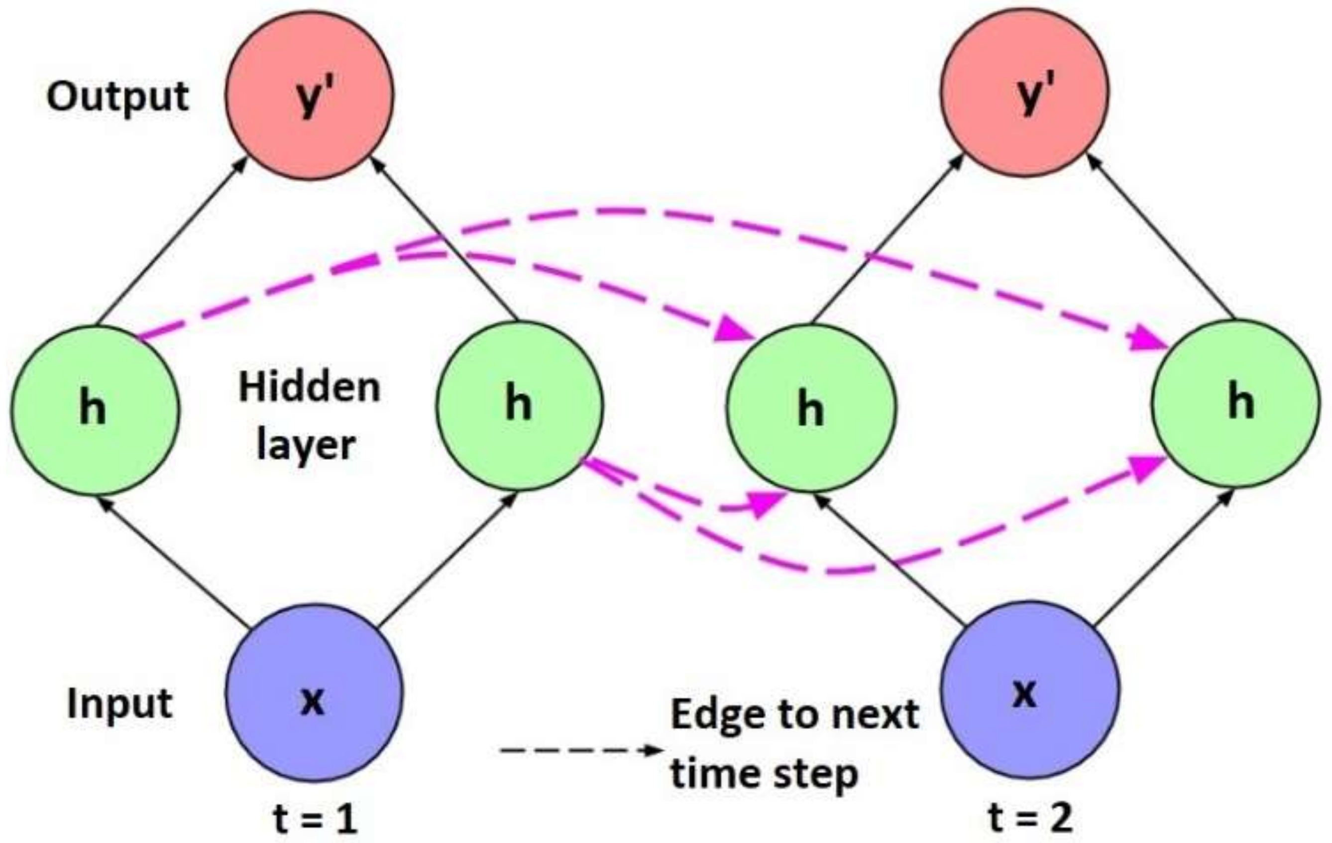
NNs with information passing across time steps are recurrent neural networks (RNN) [27]. Many applications of RNN are involved in text processing, image recognition, face detection, speech-to-text systems… At time t, nodes receive input information from the present node x(t) and information from hidden nodes h(t − 1) from NN’s previous state. The output, marked with y’(t), will be produced using that step’s hidden state, marked with h(t). Using recurrent connections, the input x(t − 1) at time t − 1 can affect the output y’(t) at time t. An example of a recurrent NN unfolded across time steps is shown in Figure 3.
Recurrent network training is considered to be difficult since its problems of exploding gradients. It occurs when errors propagate across time steps. Considering the input passed to the network at time t1 and an error occurring at time t, the input’s impact at time t1 on the output at time t will explode as t − t1 grows.
The NN’s performance was evaluated using mean square error, which is the mean of the squared difference between the actual and the estimated value. The MSE was calculated using cross-validation in which 70% of the data were used for training, and 15% for validation and testing. The MSE for each NN model is shown in Table 3.
4. Results
4.1. Bicycle Routes Created with NN-s
In addition to the MSE calculation, we evaluated the performance of our NN by cross-checking two different models. From the assumption that human experience in defining Vrgorac and Knin bicycle routes were similar, we checked if the NN models built on these routes would give consistent results, so we cross-checked them. We used the Vrgorac NN model to create routes on the Knin area and then compared them to the actual human-made routes on the Knin area. Vice-versa, we used the Knin NN model to create routes on the Vrgorac area and then compared them to the actual human-made routes on the Vrgorac area. The results obtained gave a piece of information about the representativity of our NN models.
GIS multiple-criteria model was based on points of interest, which were used as stops in route calculation. Thus, it was needed to choose locations in Vrgorac and Knin, which will be included in calculated routes as stops. There was uncertainty about how the points are going to be distributed. The shape of all the routes provided on websites [24,25], which were used as ground truth, is circular. Based on that, it was decided to place points on edge parts of routes. The aim was to use as few points as possible. All routes, except Vrgorac flat, needed three points to obtain the same or similar route as the ground truth one. Since the ground truth routes were circular, the additional one point was required to make a start and end location at the same place. Vrgorac flatter route required an extra point caused by strange ground truth route shape.
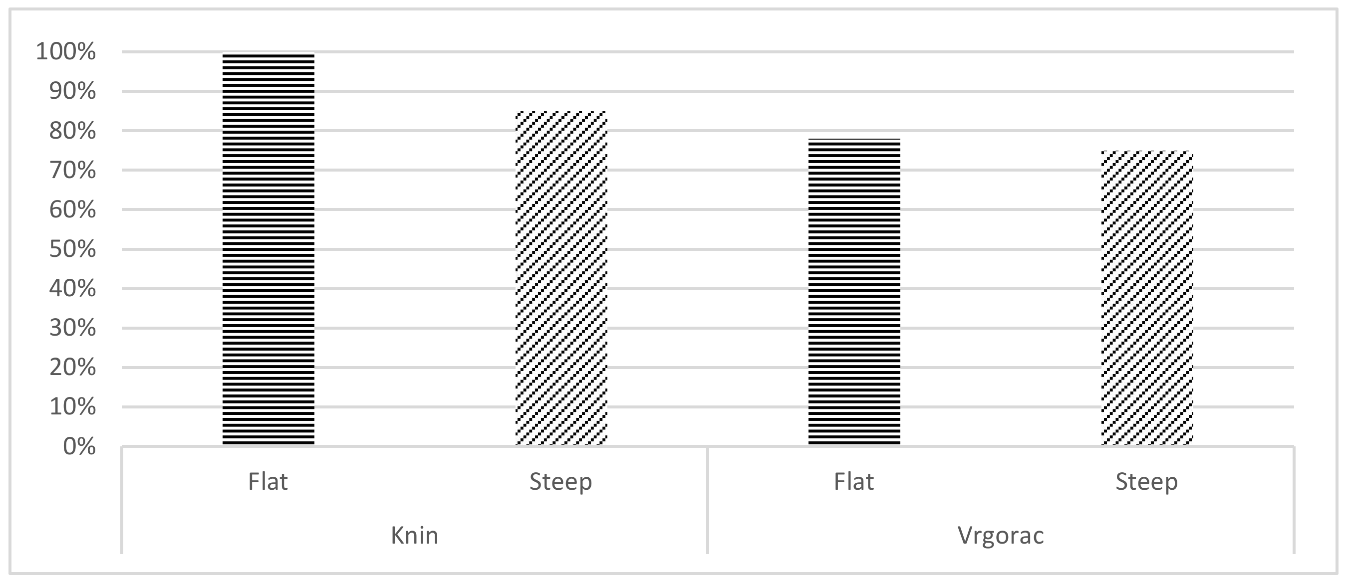
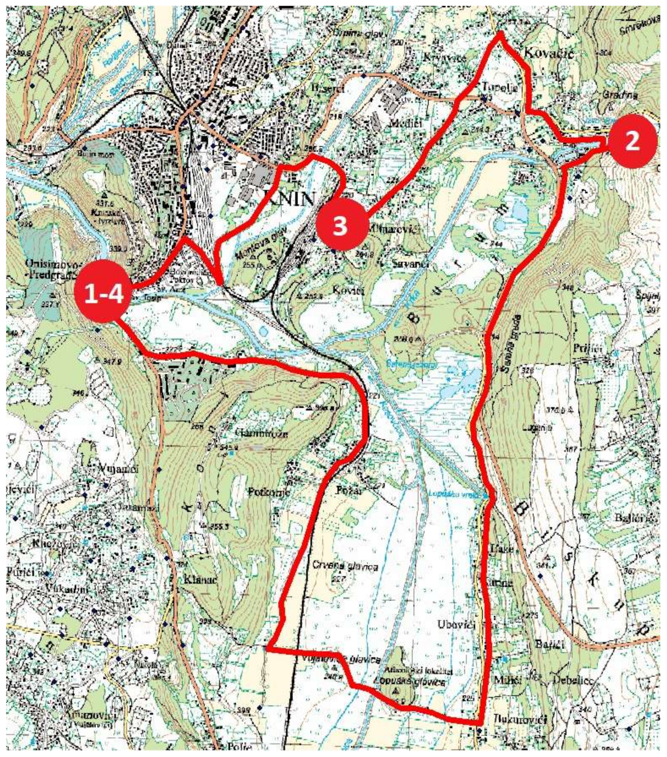
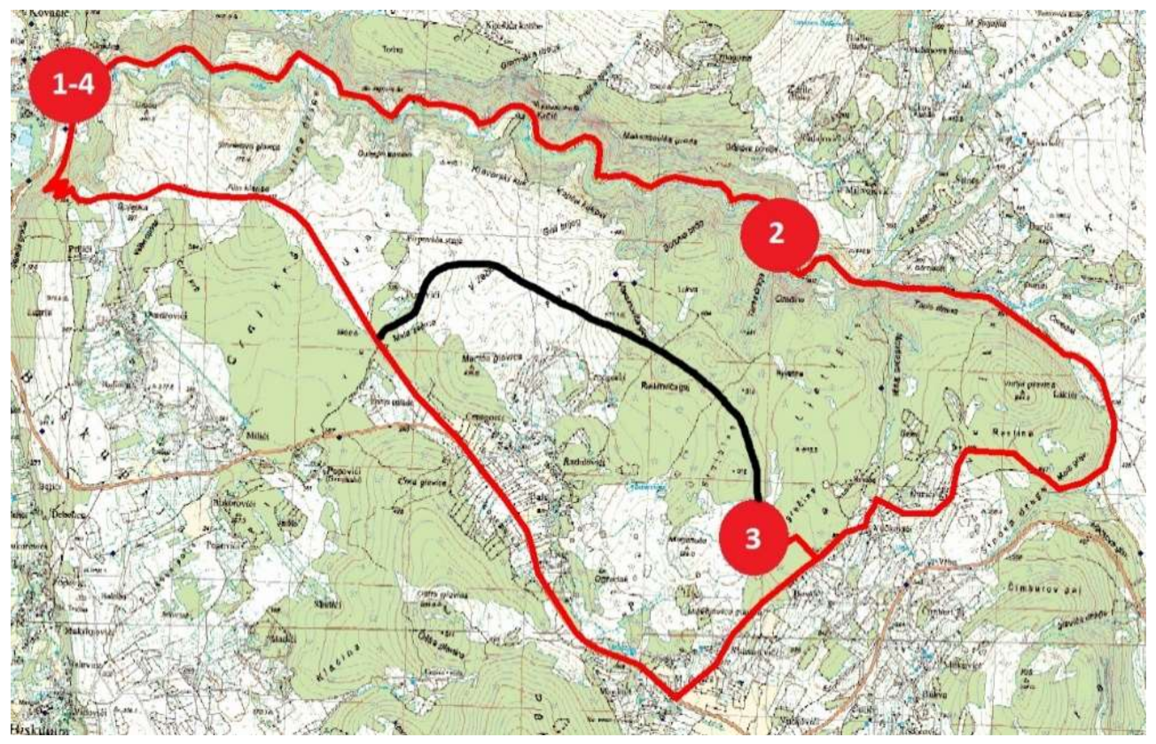
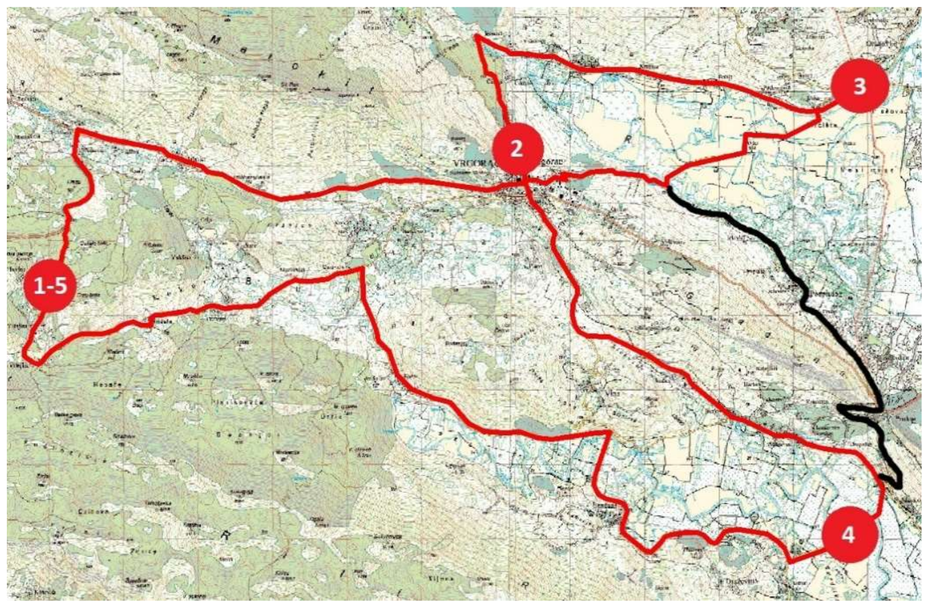
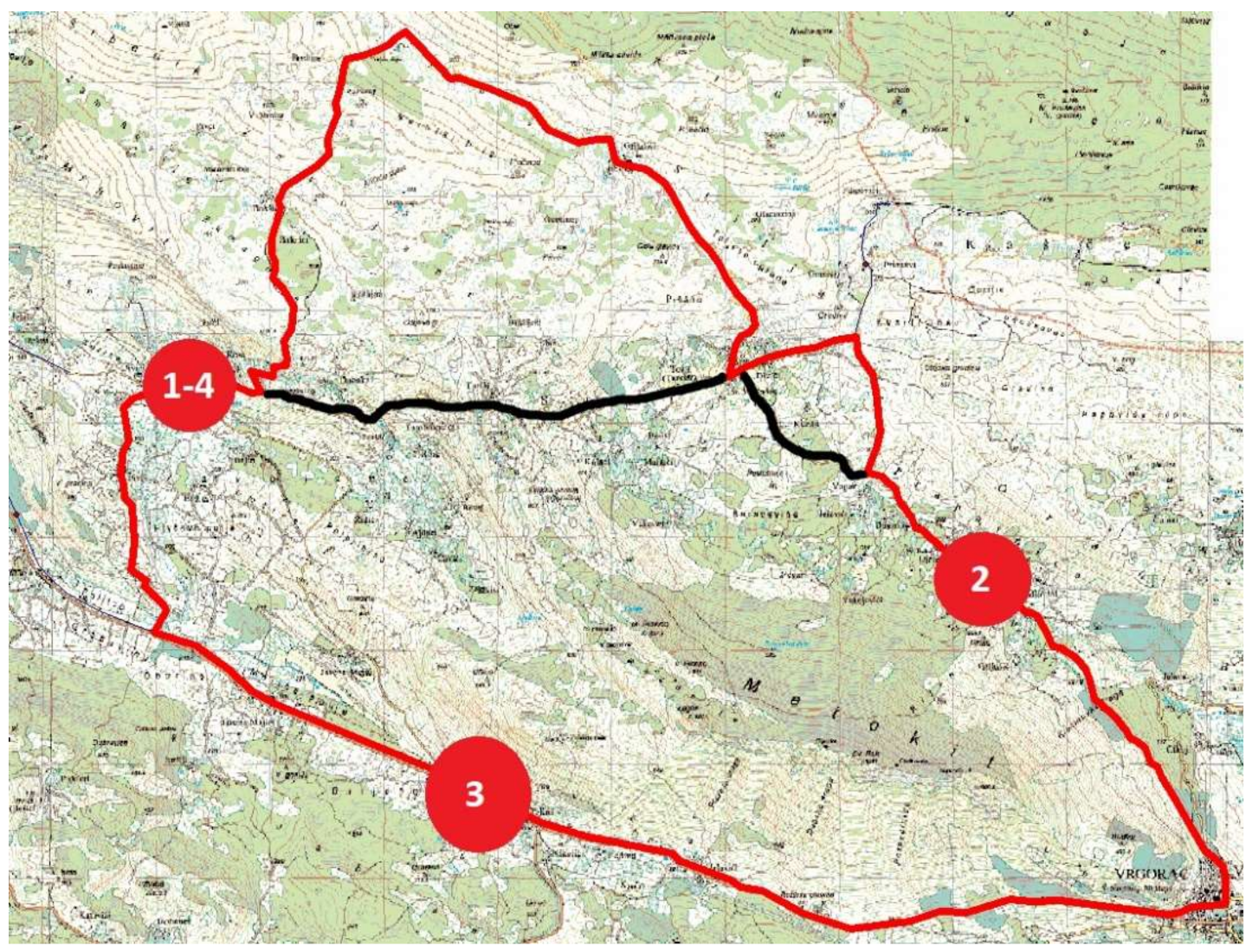
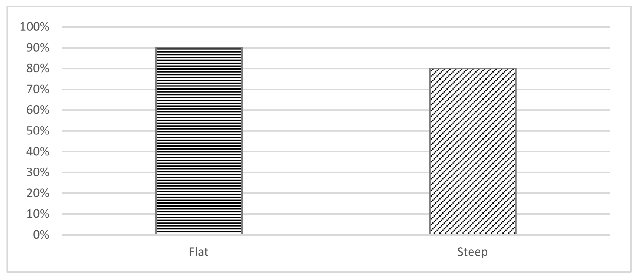
Graphical representation of the percentage of length overlapping provided in Table 4 is shown in Figure 4. Results in Table 4 and Figure 5, Figure 6, Figure 7 and Figure 8 show that there is a significant similarity between the routes produced using different models. The route NN chooses is marked with red, along with used stops, while the non-overlapping part of the route is marked with black colour. To measure the similarity, we used two metrics—the number of segments that overlapped and the length of the overlapped segments. The Vrgorac flat model used on Knin gave the identical route as the ground truth (Figure 5). For the steep Knin route, 5 of 8 segments overlapped with the ground truth route, and 85% of the route length overlapped (Figure 6). Vice versa, using the flat Knin model on Vrgorac roads provided 78% overlapping in length (18 of 21 segments) with the ground truth route (Figure 7). Using the steep Knin model on Vrgorac roads, 75% of the length (14 of 17 segments) of the steep road overlapped with the ground truth route (Figure 8). From the data shown in Table 4, it can be concluded that NN models trained in the area of Vrgorac and Knin provide a good representation of the desirability of individual bicycle paths, especially for flatter paths.
4.2. Bicycle Routes for Imotski Created by the Multicriteria Analysis
Besides using NNs for bicycle routes planning, we decided to use another classical MA GIS analysis approach. We first built the bicycle route models based on GIS in this approach, and then we used them for the best route calculation based on MA. The model chose the road segments the bicyclists will use and the order of stops to provide the best route.
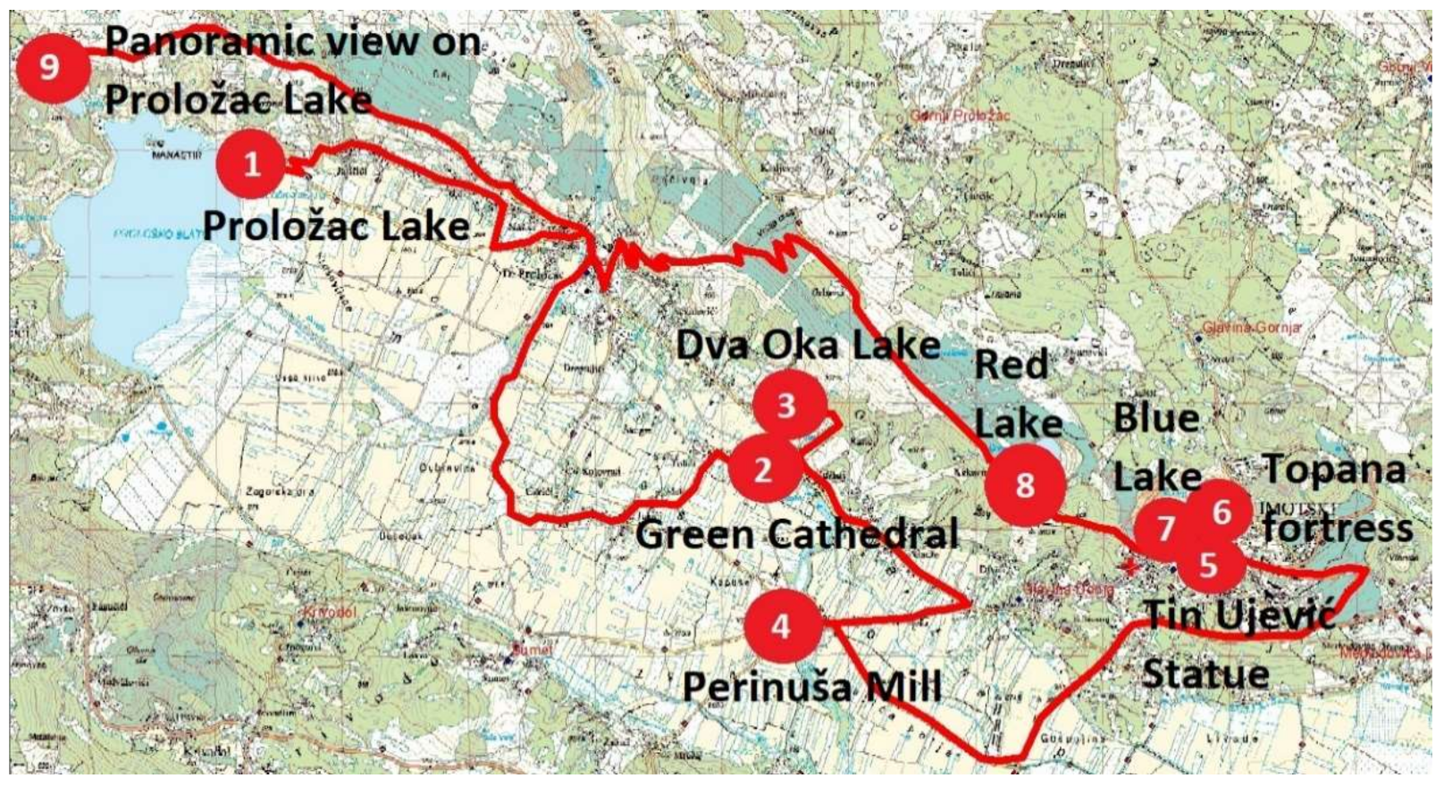
For calculating the path in which the lower slope gradient is preferable, we used the first model; the calculated path is shown in Figure 9. The path begins at the Proložac lake location, which is situated in the west part of the Imotski field. The Green Cathedral is the next stop, and the path that connects these two stops is situated at the centre of the Imotski field. Despite this route being longer, its steep gradient is lower, so it is more appropriate for non-professional cyclists. The route proceeds with Dva oka lake. Its distance to the Green Cathedral is short, and the model had no choice here since the selected route is the only one. The next stop is Perinuša mill; the model selected the route located in the Imotski field, which is the flattest part of the Imotski area. The next stop is located in the Imotski’s downtown, where the Tin Ujević’s statue is placed. A significant part of the selected route is in the main road category. This route is selected primarily because of safety-related criteria, which prefers road higher category road types. Topana fortress, Blue Lake and Red Lake are the next chosen stops. Since they are situated nearby each other, the remoteness between stops criterion prevails over other criteria. The path finished on the Panoramic view on the Proložac lake stop. Even though this path is steep, it is chosen because there was no other appropriate path between them. The substitute path’s length is too long to make that route undesirable.
We designed the second model so it could provide paths that would be more challenging; it prefers longer and steeper paths. The slope value of road segment normalised weight was inverted using the equation:
where Xi′ presents the new road segment distance weight value, and Xi is the old road segment distance; a lower weight will have the road segments with greater length.
The results of the second model are presented in Figure 10. The Perinuša mill is the first stop, preceded by Dva oka Lake and Green Cathedral, positioned in the Imotski field area with a low slope gradient. The next stops are Red Lake, Blue Lake, Imotski fortress, and Tin Ujević’s statue. The chosen path between previously mentioned stops is mostly going over the steep part of Imotski. The following two stops are a panoramic view on Proložac lake, followed by Proložac lake. Selection and scheduling of these two last stops also show that the steeper routes and the longer ones are preferred.
4.3. Bicycle Routes for Imotski Created by the Neural Networks
After cross-checking NNs trained on Vrgorac and Knin area presented in Section 4.1, we used them to model non-existing bicycle routes in the Imotski area. We compared Imotski routes calculated with NNs to ones calculated using MA.
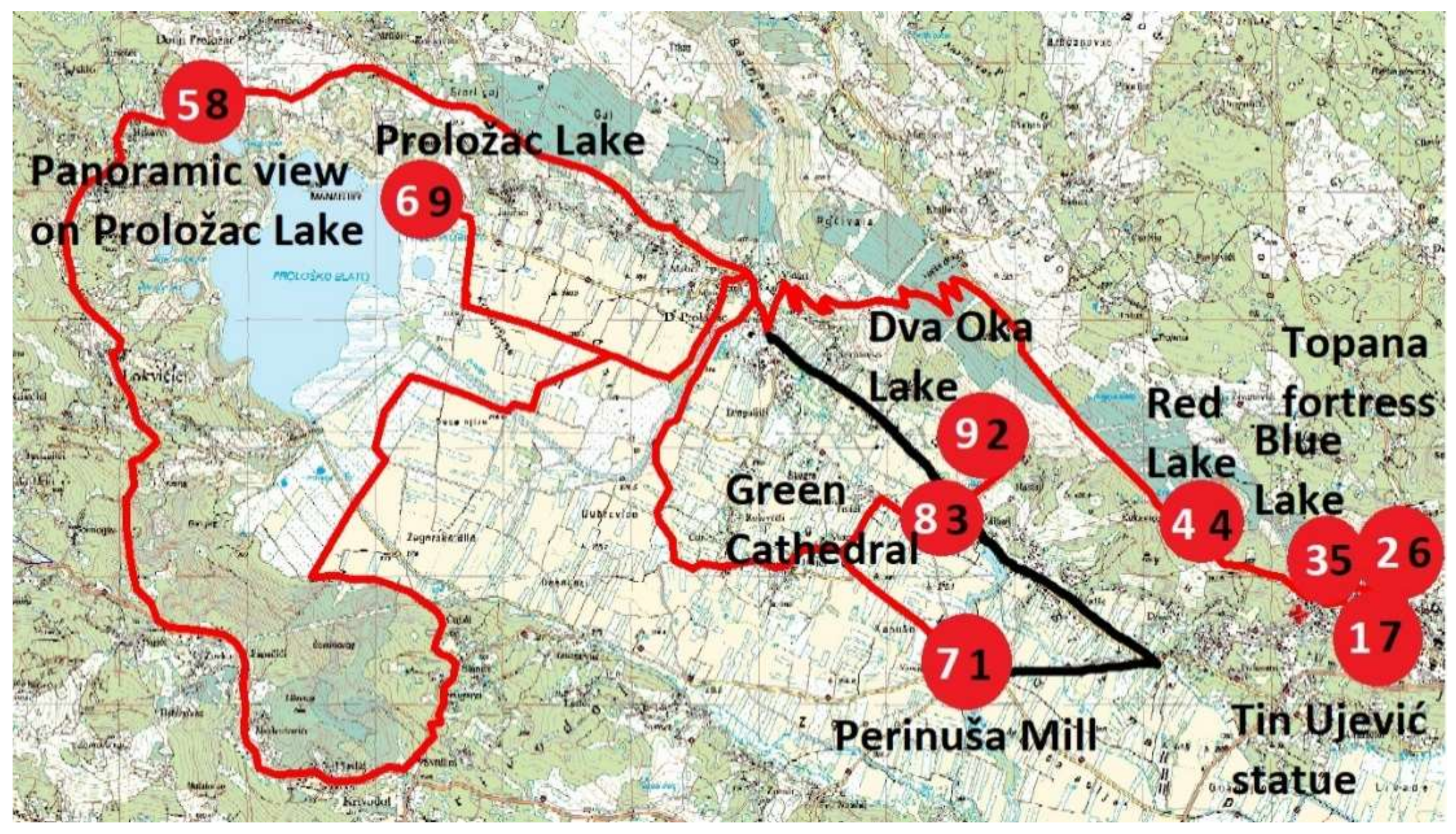
The NN provided by training on the Vrgorac area produced the flatter route 35,660 m long, of which 3788 m differs from the route calculated using MA. In total, 89% of the route calculated with the NN overlaps with the route calculated using the multicriteria approach. The route consisted of 29 segments, of which 22 was overlapping with the route calculated using the MA approach. Figure 11 compared the results produced with NN and those produced with MA when the flatter routes are preferred.
The route given by layer recurrent NN is displayed in red. The route calculated using MA that differed from the NN route is presented in black. The stop order of the NN model is labelled with white numbers, and the stop order calculated MA is labelled with black numbers. We can see that the routes overlap in most of the road network, but the stop order is different. The stop order difference is caused by the difference in the chosen route between the Imotski field and the town centre. However, we can say that both approaches gave very similar results.
The steeper route chosen by layer recurrent NN is 39,138 m long and consists of 25 segments. The part of the route, which is 7841 m long and consisted of three segments, is not the same as the route provided by MA. That means that the overlap in length between the two routes is 80%; the overlap in the number of segments is 88%.
Figure 12 presents the route calculated using a layer recurrent NN but with a network in which the steeper routes are preferred. A complete comparison of routes produced by a model trained with GIS MA and Vrgorac NN is shown in Table 5, and a graphical representation of the overlapping percentage is shown in Figure 13.
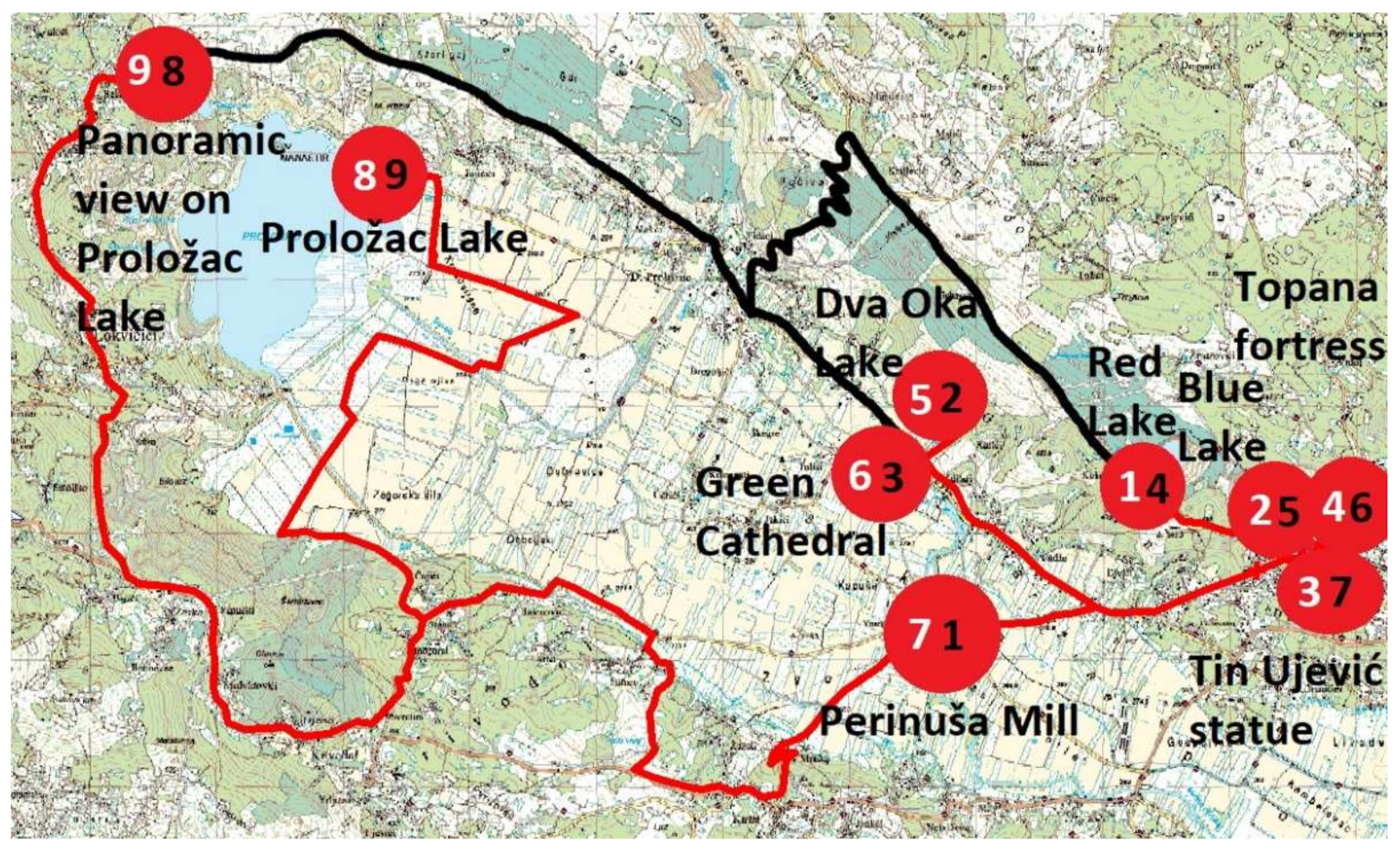
The next step was to check the results provided by models trained in the Knin area. The model which was trained on flatter routes produced the identical route on the Imotski area as the model trained on the Vrgorac area. The model trained on steeper routes provided the route shown in Figure 14, marked with black colour.
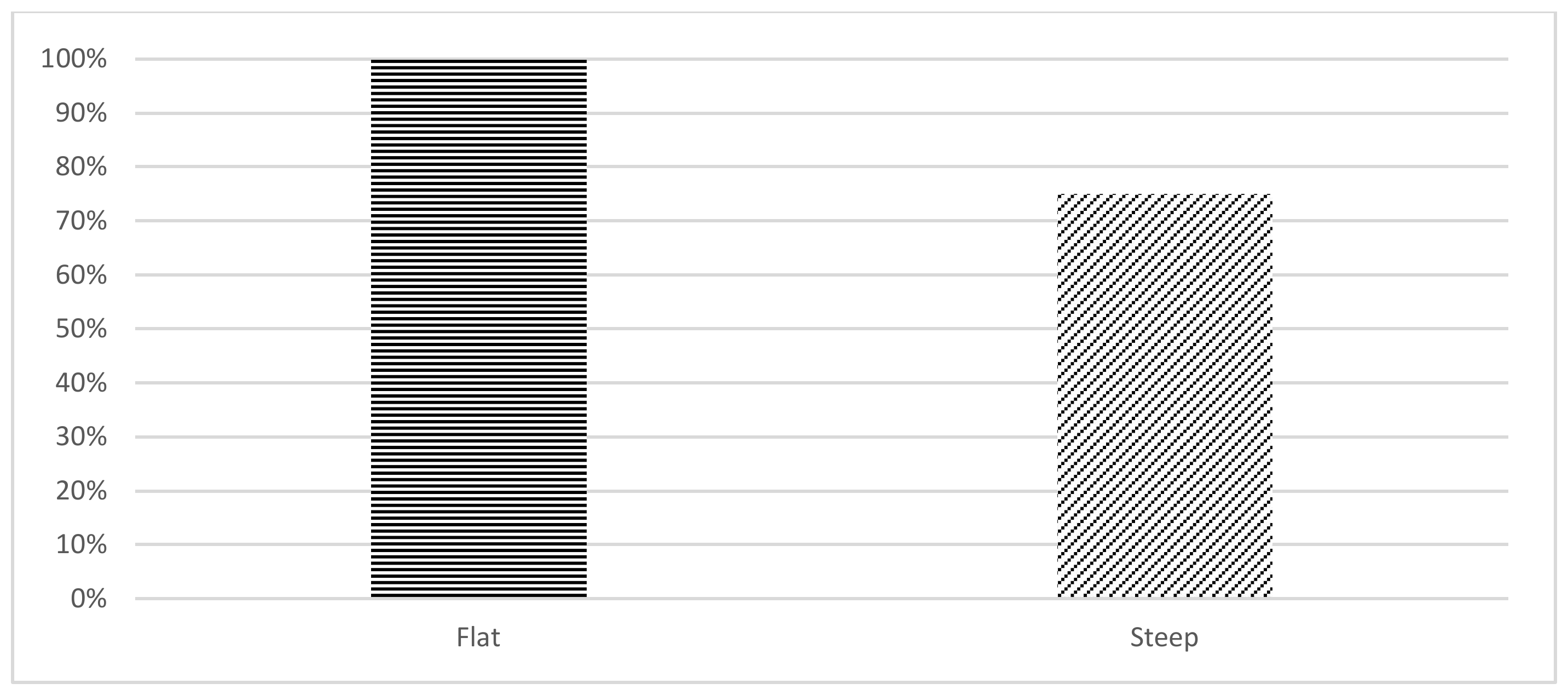
It was already stated that the steeper route chosen by layer recurrent NN is 39,138 m long and consisted of 25 segments. The part of the route, which is 9850 m long and consisted of 7 segments, is not the same as the route provided by MA. That means that the length overlap between the two routes is 75%, while the segment overlap is 72%. A complete comparison of routes produced by a model trained on Vrgorac roads with routes produced by a model trained on Knin roads is shown in Table 6, and a graphical representation of the overlapping percentage is shown in Figure 15.
5. Discussion
This paper wanted to test the use of the NNs for bicycle route planning because it would allow the transfer of human expertise in bicycle route selection from already established routes to new ones. The two models were trained: one on the data containing Knin roads; another on the data containing Vrgorac roads. We evaluated the NN performance by creating the bicycle paths in the Knin area using the Vrgorac model and vice versa.
The evaluation showed a high percentage overlapping between the NN created routes and the human-made bicycle routes in the target area. In some scenarios, the NN produced exactly the same result as the human experts, and the worst result was 75% overlap.
From this, we concluded that NN performs well and that the trained models are not overfitted. Furthermore, using the adaption learning function in the NN training process also included a bias learning function, which prevented overfitting.
We evaluated the NN performance using MSE calculation; it was used for all models, and the steep Vrgorac model had the biggest MSE of 0.0809. However, even though this calculation indicated our model’s quality, since the models are used on roads in different areas, we think that the final quality indicator was a cross-validation check that was previously mentioned.
One of the primary inputs to the NN was the TIN relief model. It was reconstructed using layers with a height data resolution of 50 m. Thus, the resolution of the elevation model depended on how the steep ground was, meaning that the higher resolution was in places where the surface is more variable.
When calculating the distance between each segment and the emergency unit and water source, it was decided to consider the segment as a point located at the centre of the segment. This was a compromise between the precision and calculation time. It primarily affected the calculation of the distance to a water source. The water source we used was a polyline, and it was needed to find the nearest water source segment to each road segment. Using all points the polyline consists of to present the segment would make the calculation very time-consuming. In our model, the mean length of the segment was 1556.06 m, while the mean distance to the emergency unit and water source is 22,388.26 m.
Besides the experiment in which we checked the ability of two NN models trained on different areas to produce good bicycle paths, we compared the paths created by those two models to the paths created by classical GIS MA on the Imotski area. In MA, the essential question was whether the selected criteria and the assigned weight reflects what affects the cyclist’s choice of bicycle route in reality. The higher weight was assigned to the slope grade because we considered it the most crucial criterion for bicycle route usage, especially for amateur cyclists.
The paths created by two NNs matched well with the paths created by GIS MA. Thus, we concluded that (1) the criteria for GIS MA was well chosen, and (2) that no overfitting is present in our NN model. If overfitting were present in these two networks, they would be over-specialised on their (different) training sets, and then they would produce different predictions on the third data set, which was not the case.
Even though the MA and NN match was close, there were still minor differences between selected routes using different methods. The differences can be affected by the fact that more criteria affect the bicycle route selection than those considered in this paper and the fact that in MA selection of criteria and weights assigned to each criterion were not perfect.
6. Conclusions
Bicycle route planning with NN usage is presented in this paper. A set of already established bicycle routes is used for the NN training, which enabled the transfer of bicycle route design human expertise into a NN. Then the trained NN is used to design the routes on a novel area. We trained NNs in two different areas which were capable of choosing the best route among the given road network.
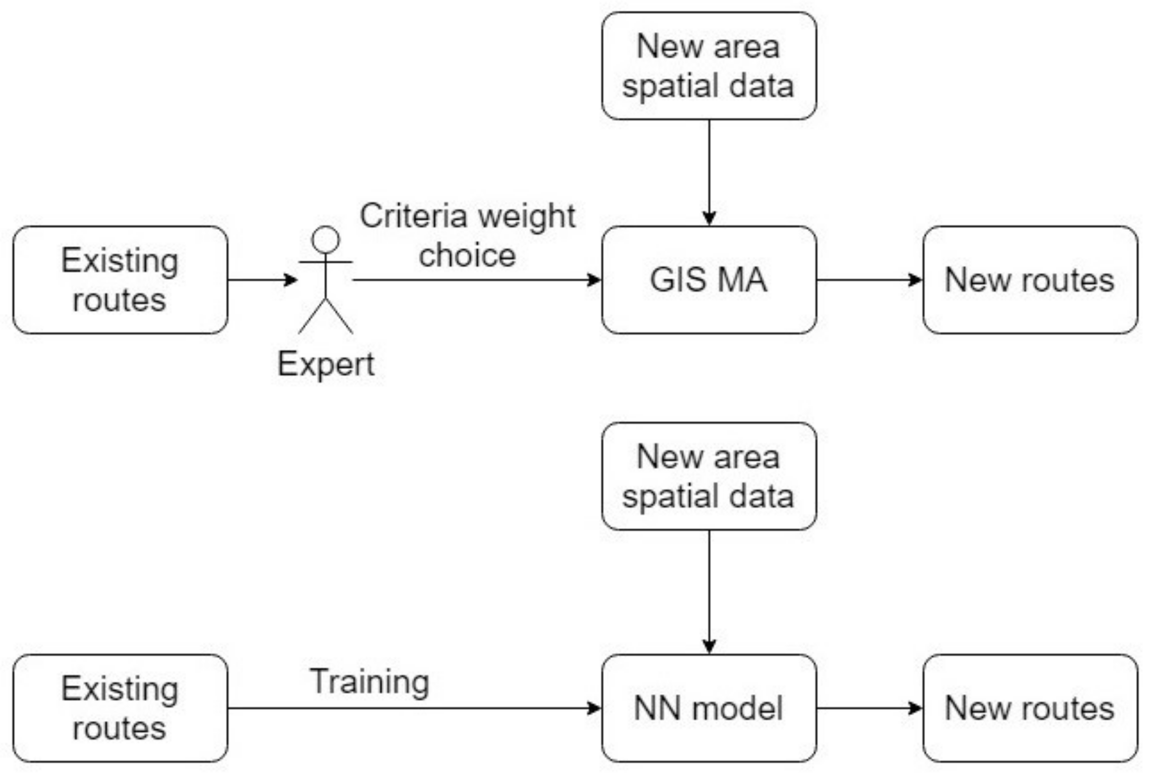
This paper dealt with a different approach to dealing with the most appropriate bicycle route in a rural area. In literature research, most of the papers dealt with bicycle routing problems in an urban area but primarily relied on GIS or NN separately. This is the reason why we decided to join these two approaches. While MA needed an expert to decide which criteria should be used, the NN approach made it possible to have expertise concentrated in NN. It is crucial that we have shown that the model is usable not only in the Imotski area but also in the area of the Dalmatian hinterland, maybe even broader. The visualisation of the conclusion is shown in Figure 16.
The NN approach showed that it could be successfully used for bicycle route prediction. Considering the roads segment data as the input in the NN, we decided to use the layer recurrent NN. We then trained two NNs on existing routes in two areas (Vrgorac and Knin) that are similar by their characteristics. We cross-checked routes Vrgorac NN selected on existing Knin routes and vice-versa, and they overlapped on average of 84% of their length.
Besides this, we used the classical GIS multiple criteria approach to check the NN approach. The target area for our experiment of bicycle route planning was a broader area of the city of Imotski, which is a mix of small urban and rural areas. We created two routes using both modelling approaches: the first one shorter and flatter, targeted at amateurs and tourist bicyclists, and the second one longer and steeper, targeted at enthusiasts. Then we used the Knin and Vrgorac NNs to build networks for the Imotski area and analysed how the results overlap with routes created by MA. The flat routes created with Knin and Vrgorac NNs were identical and, compared to the GIS MA route, were 90% similar. The steeper routes of Knin and Vrgorac were 75% similar, and the overlap with GIS MA was 80%.
We can conclude that the NN approach to modelling bicycle routes is more direct and faster since, in MA, a bicycle expert has to choose criteria and adjust its weights carefully. In contrast, the NN method extracts them automatically from existing routes.
Future work will include the real-world corroboration of the Imotski routes presented in this work. It is planned to use affective computing equipment to acquire data about the emotional state of cyclists who will use the chosen bicycle path, which will provide feedback about the desirability of the path in the real world.
Although we chose the area with highly dynamic terrain, we are unsure that the trained model would suit areas with different terrain configurations. Therefore, it would be interesting to train a model in some other areas, e.g., the Slavonia area, the vastest Croatian plain. That might give us insight into the sensitivity of our model to the terrain dynamic.
The future work considering NN will be based on building a bigger training model and experimenting with NNs based on bicycle paths and not route segments.
Since the safety-related factors are the most noteworthy in bicycle path selection, our work in the future will include traffic density as a criterion to evade car-congested parts of roads.
Author Contributions
J.Đ.: Conducted research conceptualisation, data acquisition, provided methodology, validated results, wrote the original draft, reviewed and edited draft. M.S.: supervised, advised, validated the multicriteria methodology, analysed results, reviewed and edited draft. L.K.: validated neural network methodology, analysed results, reviewed and edited draft. M.R.: supervised, advised, validated the multicriteria and neural network methodology, analysed results, reviewed and edited draft. All authors have read and agreed to the published version of the manuscript.
Funding
Supported by the Virtual Telemedicine Assistance—VITA, a project co-financed by the Croatian Government and the European Union through the European Regional Development Fund-the Competitiveness and Cohesion Operational Programme (KK.01.1.1.01).
Institutional Review Board Statement
Not applicable.
Informed Consent Statement
Not applicable.
Data Availability Statement
If interested, the data used in this work can be provided. ArcGIS and Matlab software were used. There are only a few lines of code used only in Multicriteria analysis in assigning weights to criteria. If interested, the code can be provided.
Conflicts of Interest
The authors declare no conflict of interest.
References
- Latifi, R.; Hadeed, G.J.; Rhee, P.; O’Keeffe, T.; Friese, R.S.; Wynne, J.L.; Ziemba, M.L.; Judkins, D. Initial experiences and outcomes of telepresence in the management of trauma and emergency surgical patients. Am. J. Surg. 2009, 198, 905–910. [Google Scholar] [CrossRef] [PubMed]
- Miller, A.C.; Ward, M.M.; Ullrich, F.; Merchant, K.A.; Swanson, M.B.; Mohr, N.M. Emergency Department Telemedicine Consults are Associated with Faster Time-to-Electrocardiogram and Time-to-Fibrinolysis for Myocardial Infarction Patients. Telemed. e-Health 2020, 26, 1440–1448. [Google Scholar] [CrossRef] [PubMed]
- Yegnanarayana, B. Artificial Neural Networks; Prentice-Hall of India: Hoboken, NJ, USA, 2006. [Google Scholar]
- Basheer, I.A.; Hajmeer, M. Artificial neural networks: Fundamentals, computing, design, and application. J. Microbiol. Methods 2000, 43, 3–31. [Google Scholar] [CrossRef]
- Jain, A.K.; Jianchang, M.; Mohiuddin, K.M. Artificial neural networks: A tutorial. Computer 1996, 29, 31–44. [Google Scholar] [CrossRef] [Green Version]
- Đerek, J.; Sikora, M. Bicycle route planning using multiple criteria GIS analysis. In Proceedings of the 2019 IEEE 27th International Conference on Software, Telecommunications and Computer Networks (SoftCOM), Split, Croatia, 19–21 September 2019. [Google Scholar]
- Hsu, T.P.; Lin, Y.T. A model for planning a bicycle network with multicriteria suitability evaluation using GIS. WIT Transactions on Ecology and the Environment 2011, 148, 243–252. [Google Scholar]
- De Grann, J.G. Extensions of the Multiple Criteria Analysis Method of T.L. Satty, A Report for National Institute for Water Supply; EURO IV.; Cambridge: Voorburg, The Netherlands, 1980. [Google Scholar]
- Csutora, R.; Buckley, J.J. Fuzzy Hierarchical Analysis: The Lambda-Max Method. Fuzzy Sets Syst. 2001, 120, 181–195. [Google Scholar] [CrossRef]
- Chen, P.; Qing, S.; Suzanne, C. A GPS data-based analysis of built environment influences on bicyclist route preferences. Int. J. Sustain. Transp. 2018, 12, 218–231. [Google Scholar] [CrossRef]
- Huang, Y.; Gordon, Y. Selecting Bicycle Commuting Routes Using GIS. Berkeley Plan. J. 1995, 10, 75–90. [Google Scholar] [CrossRef] [Green Version]
- Bi, H.; Shang, W.L.; Chen, Y.; Wang, K.; Yu, Q.; Sui, Y. GIS aided sustainable urban road management with a unifying queueing and neural network model. Appl. Energy 2021, 291, 116818. [Google Scholar] [CrossRef]
- Samarasinghe, C.K. Landslide susceptibility prediction based on GIS and Artificial Neural Network. Ph.D. Thesis, University of Colombo School of Computing, Colombo, Sri Lanka, 2021. [Google Scholar]
- Wang, Z.; Zlatanova, S.; Moreno, A.; Van Oosterom, P.; Toro, C. A data model for route planning in the case of forest fires. Comput. Geosci. 2014, 68, 1–10. [Google Scholar] [CrossRef] [Green Version]
- De Luca, M. A comparison between prediction power of artificial neural networks and multivariate analysis in road safety management. Transport 2017, 32, 379–385. [Google Scholar] [CrossRef] [Green Version]
- Sameen, M.; Biswajeet, P. Severity prediction of traffic accidents with recurrent neural networks. Appl. Sci. 2017, 7, 476. [Google Scholar] [CrossRef] [Green Version]
- Song, J.; Shengwei, Q. The Bus Line Supporting System Based On Learning Neural Network Model Applied In GIS. In Proceedings of the 2015 5th International Conference on Computer Sciences and Automation Engineering (ICCSAE 2015), Sanya, Hainan, China, 14–15 November 2015; Atlantis Press: Pleasantville, NI, USA, 2016. [Google Scholar]
- Kia, M.B.; Pirasteh, S.; Pradhan, B.; Mahmud, A.R.; Sulaiman, W.N.; Moradi, A. An artificial neural network model for flood simulation using GIS: Johor River Basin, Malaysia. Environ. Earth Sci. 2012, 67, 251–264. [Google Scholar] [CrossRef]
- Shah, S.A.; Brijs, T.; Ahmad, N.; Pirdavani, A.; Shen, Y.; Basheer, M.A. Road safety risk evaluation using gis-based data envelopment analysis—Artificial neural networks approach. Appl. Sci. 2017, 7, 886. [Google Scholar] [CrossRef] [Green Version]
- Pritchard, R.; Yngve, F.; Bernhard, S. Bicycle level of service for route choice—A GIS evaluation of four existing indicators with empirical data. ISPRS Int. J. Geo-Inf. 2019, 8, 214. [Google Scholar] [CrossRef] [Green Version]
- Grekousis, G.; Panos, M.; Yorgos, N.P. Modeling urban evolution using neural networks, fuzzy logic and GIS: The case of the Athens metropolitan area. Cities 2013, 30, 193–203. [Google Scholar] [CrossRef]
- Lenstra, J.K.; Kan, A.R. Some simple applications of the travelling salesman problem. J. Oper. Res. Soc. 1975, 26, 717–733. [Google Scholar] [CrossRef]
- Udovičić, G.; Ðerek, J.; Russo, M.; Sikora, M. Wearable Emotion Recognition System based on GSR and PPG Signals. In Proceedings of the 2nd International Workshop on Multimedia for Personal Health and Health Care, Mountain View, CA, USA, 23 October 2017; ACM: New York, NY, USA, 2017. [Google Scholar]
- Dalmatia-Bike. Available online: http://www.dalmatia-bike.com (accessed on 30 May 2019).
- Dalmacija-Šibenik. Available online: http://www.bikeandhike.hr (accessed on 14 April 2020).
- Lv, C.; Xing, Y.; Zhang, J.; Na, X.; Li, Y.; Liu, T.; Cao, D.; Wang, F.Y. Levenberg–Marquardt backpropagation training of multilayer neural networks for state estimation of a safety-critical cyber-physical system. IEEE Trans. Ind. Inform. 2017, 14, 3436–3446. [Google Scholar] [CrossRef] [Green Version]
- Lipton, Z.C.; Berkowitz, J.; Elkan, C. A critical review of recurrent neural networks for sequence learning. arXiv 2015, arXiv:1506.00019. [Google Scholar]
Figure 1.
Triangulated irregular network (TIN) relief model.

Figure 2.
Diagram with route calculation procedure explained.

Figure 3.
A recurrent network unfolded across time steps.

Figure 4.
Model verification results-percentage of the length overlap in cross-checking NNs between results of GIS MA and Vrgorac NN for Imotski bicycle routes.
Figure 4.
Model verification results-percentage of the length overlap in cross-checking NNs between results of GIS MA and Vrgorac NN for Imotski bicycle routes.

Figure 5.
Vrgorac model on Knin roads-flat.

Figure 6.
Vrgorac model on Knin roads-steep.

Figure 7.
Knin model on Vrgorac roads-flat.

Figure 8.
Knin model on Vrgorac roads-steep.

Figure 9.
Selected route-flatter route preferred.

Figure 10.
Selected route-longer distance and higher slope gradient preferred.

Figure 11.
Comparison—flatter route produced by layer recurrent NN.

Figure 12.
Comparison—steeper route produced by layer recurrent NN.

Figure 13.
Percentage of the length overlap between results of GIS MA and Vrgorac NN for Imotski bicycle routes.
Figure 13.
Percentage of the length overlap between results of GIS MA and Vrgorac NN for Imotski bicycle routes.

Figure 14.
Comparison—steeper route produced by layer recurrent NN trained in the Knin area.

Figure 15.
Percentage of the length overlap between results of Vrgorac and Knin NNs.

Figure 16.
Diagrams of MA and NN analysis approach.


Table 1.
Number of road segments for each town.
| Town | No. of Segments |
|---|---|
| Vrgorac | 168 |
| Knin | 215 |
| Imotski | 268 |
Table 2.
Model training parameters.
| Parameter | Description | Value |
|---|---|---|
| epochs | maximum number of training iterations | 1000 |
| time | maximum time of training in seconds | Inf |
| goal | performance goal in terms of the network’s performance functions | 0 |
| min_grad | minimum performance gradient | 10−7 |
| max_fail | maximum number of validation checks | 6 |
| mu | used for training with the Levenberg–Marquardt training function; the greater it is—the more weight is given to the gradient descent learning and small step size | 0.01 |
| mu_dec | amount to decrease mu after an unsuccessful step | 0.1 |
| mu_inc | amount to increase mu after a successful step | 10 |
| mu_max | maximum mu | 109 |
Table 3.
NN performance using MSE.
| Route | MSE | |
|---|---|---|
| Knin | Flat | 0.0298 |
| Steep | 0.0151 | |
| Vrgorac | Flat | 0.0572 |
| Steep | 0.0809 | |
Table 4.
Model verification results.
| Route | Route Length (Overlapping) | Number of Segments in Route (Overlapping) | Percentage of Length Overlapping | Percentage of Overlapping Segments | |
|---|---|---|---|---|---|
| Knin | Flat | 16,542 m (16,542 m) | 19 (19) | 100% | 100% |
| Steep | 36,353 m (31,010 m) | 8 (5) | 85% | 62.5% | |
| Vrgorac | Flat | 42,420 m (33,293 m) | 21(18) | 78% | 86% |
| Steep | 25,021 m (19,766 m) | 17 (14) | 75% | 82% | |
Table 5.
Comparison of Imotski bicycle routes given by model trained with GIS MA and a NN trained in Vrgorac area.
Table 5.
Comparison of Imotski bicycle routes given by model trained with GIS MA and a NN trained in Vrgorac area.
| Type of Route | Route Length (Overlapping) | Number of Segments in Route (Overlapping) | Percentage of Length Overlapping | Percentage of Overlapping Segments |
|---|---|---|---|---|
| Flat | 35,660 m (31,872 m) | 29 (22) | 89% | 76% |
| Steep | 39,318 m (31,477 m) | 25 (22) | 80% | 88% |
Table 6.
Comparison of route given by model trained on Vrgorac roads with route given by model trained on Knin roads.
Table 6.
Comparison of route given by model trained on Vrgorac roads with route given by model trained on Knin roads.
| Type of Route | Route Length (Overlapping) | Number of Segments in Route (Overlapping) | Percentage of Length Overlapping | Percentage of Overlapping Segments |
|---|---|---|---|---|
| Flat | 35,660 m (35,660 m) | 29 (29) | 100% | 100% |
| Steep | 39,318 m (29,468 m) | 25 (18) | 75% | 72% |
Publisher’s Note: MDPI stays neutral with regard to jurisdictional claims in published maps and institutional affiliations. |
© 2021 by the authors. Licensee MDPI, Basel, Switzerland. This article is an open access article distributed under the terms and conditions of the Creative Commons Attribution (CC BY) license (https://creativecommons.org/licenses/by/4.0/).
Share and Cite
MDPI and ACS Style
Đerek, J.; Sikora, M.; Kraljević, L.; Russo, M. Using Neural Networks for Bicycle Route Planning. Appl. Sci. 2021, 11, 10065. https://doi.org/10.3390/app112110065
AMA Style
Đerek J, Sikora M, Kraljević L, Russo M. Using Neural Networks for Bicycle Route Planning. Applied Sciences. 2021; 11(21):10065. https://doi.org/10.3390/app112110065
Chicago/Turabian StyleĐerek, Jurica, Marjan Sikora, Luka Kraljević, and Mladen Russo. 2021. "Using Neural Networks for Bicycle Route Planning" Applied Sciences 11, no. 21: 10065. https://doi.org/10.3390/app112110065
Note that from the first issue of 2016, this journal uses article numbers instead of page numbers. See further details here.