
Shark Skin—An Inspiration for the Development of a Novel and Simple Biomimetic Turbulent Drag Reduction Topology

1
School of Naval Architecture, Ocean and Energy Power Engineering, Wuhan University of Technology, Wuhan 430063, China
2
Guangdong Electric Power Design Institute Co., Ltd. of China Energy Engineering Group, Guangzhou 510530, China
3
Green & Smart River-Sea-Going Ship, Cruise and Yacht Research Center, Wuhan University of Technology, Wuhan 430063, China
4
Guangxi Key Laboratory of Ocean Engineering Equipment and Technology, Beibu Gulf University, Qinzhou 535000, China
5
College of Science and Engineering, Flinders University, Adelaide 5042, Australia
*
Author to whom correspondence should be addressed.
Sustainability 2022, 14(24), 16662; https://doi.org/10.3390/su142416662
Submission received: 8 November 2022
/
Revised: 5 December 2022
/
Accepted: 6 December 2022
/
Published: 13 December 2022
(This article belongs to the Special Issue Sustainable Hydrodynamic Modelling in Offshore and Ocean Engineering)
Abstract
:In this study, a novel but simple biomimetic turbulent drag reduction topology is proposed, inspired by the special structure of shark skin. Two effective, shark skin-inspired, ribletted surfaces were designed, their topologies were optimized, and their excellent drag reduction performances were verified by large eddy simulation. The designed riblets showed higher turbulent drag reduction behavior, e.g., 21.45% at Re = 40,459, compared with other experimental and simulated reports. The effects of the riblets on the behavior of the fluid flow in pipes are discussed, as well as the mechanisms of fluid drag in turbulent flow and riblet drag reduction. Riblets of various dimensions were analyzed and the nature of fluid flow over the effective shark skin surface is illustrated. By setting up the effective ribletted surface on structure’s surface, the shark skin-inspired, biomimetic, ribletted surface effectively reduced friction resistance without external energy support. This method is therefore regarded as the most promising drag reduction technique.
1. Introduction
The skin of fast swimming sharks is known to reduce skin friction drag in the turbulent flow regime, while small eddies that occur around the sharks’ bodies make it difficult for microscopic aquatic organisms to adhere to the sharks’ surface [1]. Scientists have carried out in-depth studies exploring shark skin. It has been found that shark skin gains excellent drag reduction performance due to its non-smooth surface. The shape of the riblets on the skin surface greatly influences the effectiveness of drag reduction, with ribletted surfaces performing best when aligned parallel to the flow direction. Moreover, riblets with a sharp tip show optimal reduction of wall shear stress [2]. Experts have conducted much research investigating the optimal morphology of drag reduction. The effects of the dimensions (including s+, h+, etc.) and shapes of different riblets, the flow field, and the yaw angle (γ) on turbulent drag reduction have become the focus of research, since excellent performance and significant development prospects have been scientifically demonstrated by many experimental and numerical studies. In a classic experiment, Bechert et al. investigated drag reduction using a plastic model surface of compliant shark scales with riblets [3]. The surface consisted of 800 individual movable scales, allowing different angles of flow attack to be simulated. The achievable wall shear stress reduction was 3%. Lee and Lee [4] reported various effects of a non-smooth surface with different sizes of circular concavities on near-wall turbulence (reduced drag when s+ = 25.2 and increased drag when s+ = 40.6). Djenidi and Antonia [5] applied laser Doppler anemometry to investigate flow over surfaces with V-shaped riblets and found that the riblets could decrease and increase drag when s+ = 25 and s+ = 75, respectively. The linear relationship between drag reduction and the non-dimensional parameter of the rectangular riblet in pipe flow was proven by Rapp [6] in 2006. With well-designed experiments in an oil tank, Bechert et al. [1] investigated the drag reduction performance of different riblet shapes, including triangular, trapezium, and blade-shaped riblets. The results showed that blade-shaped riblets, which reduced turbulent shear stress by 9.9% compared to smooth surfaces when h = 0.5 s, had the best drag reduction performance. Wang et al. [7] experimented with four different types of riblets and found excellent drag reduction performance, with the maximum reduction being 26%. Comparative studies by Cong et al. [8] on drag reduction and turbulent flow over triangular, scalloped, and blade-shaped riblets showed that the drag of these three bionic non-smooth surfaces was smaller than that of smooth surfaces, with blade-shaped riblets producing the greatest drag reduction and scalloped riblets producing the second greatest. Researchers including Choi [9], Debisschop and Nieuwstadt [10], Wang et al. [11], and Cong and Feng [12] have researched the effect of the pressure gradient of the flow field on drag reduction, but no general agreement has yet been reached. There have also been elaborate investigations of the differences between longitudinal and transverse non-smooth surfaces. Paolo et al. [13] employed numerical methods to study the general aspects of flows over transverse and longitudinal regular sinusoidal, triangular, and parabolic riblets. Fukagata [14] experimentally found that drag decreased over longitudinal wavy surfaces.
Thus far, much research has been conducted exploring the reduction of turbulent drag over non-smooth ribletted surfaces of flat plates, and remarkable advances have been made. However, much less research has been conducted on the reduction of turbulent drag over biomimetic ribletted surfaces inside pipes. Nitschke [15] investigated air flow in pipes with riblets with rounded peaks machined into their interior surface by measuring the pressure drop. It was found that riblets reduced drag when s+ = 8~23 and the maximum drag reduction was gained when s+ = 11~15. Nevertheless, some researchers pointed out that the riblets with rounded peaks that Nitschke used did not produce the greatest effects in reducing turbulent drag on flat plates in the developing external flows. Chen and Leung [16] performed a series of experiments with three different types of ribletted surface and proved that all three longitudinal surfaces achieved drag reduction in internal turbulent flow. In a comparative experiment, Reidy and Anderson [17] applied sharply peaked, symmetrical, triangular riblets manufactured by 3M Company to both flat plates and the inside of a six-inch pipe. The results showed that the drag reduction in internal turbulent flow was three times that in external turbulent flow. Enyutin et al. [18] studied fully developed turbulent air flow in a pipe with different types of riblets and reported a maximum drag reduction of 5~6%. In that experiment, the authors again proved that surfaces with triangular riblets showed better drag reduction performance than ribletted surfaces with rounded peaks. Shiki et al. [19] made further progress in this direction. These authors analyzed the velocity profile, static pressure, and flow rate of triangular riblets of different shapes and sizes in a fully developed turbulent pipe flow. The pipe was 492 mm in interior diameter and 4000 mm in length, with Reynolds number flows between 3.0 × 10⁵ and 8.0 × 10⁵, and the maximum drag reduction gained was 8% at approximately h+ = 11.4. The authors thereby deduced the optimum geometrical shape and size of riblets for turbulent drag reduction in pipes.
Along with deeper research, progress has been made regarding three dimensional riblets. Koeltzsch et al. [20] investigated the turbulent drag reduction performance of divergent and convergent riblets in pipe flow, yielding enlightening information about turbulent drag reduction over non-smooth surfaces of pipes. In 2010, Auteri et al. [21] performed experiments investigating the drag reduction performance of a travelling wave surface in turbulent pipe flow, reporting a maximum drag reduction as high as 33%. This surprising finding was confirmed in 2011 in a wind tunnel experiment by Tang et al. [22] with a longitudinal travelling wave surface. Ahn et al. [23] used large eddy simulation (LES) of the flow field and thermal transmission of pipes with rectangular and circular riblets. Peet and Sagaut [24] used a numerical simulation in their study of longitudinal triangular and sinusoidal riblets in pipe flow, reporting that the drag reduction of sinusoidal riblets was 50% greater than that of longitudinal triangular riblets. Martin and Bhushan [25] used a numerical simulation in their study of a closed channel to directly compare flat and ribletted surfaces. The drag and vortex formations were analyzed and compared to a flat surface and other continuous riblet configurations. The relationship between vortex dimensions and riblet geometry were explored both for continuous and segmented configurations. An optimization modeling study of various riblet geometries to achieve low drag was performed by Martin and Bhushan [26]. A shark-inspired scalloped geometry was additionally modeled to compare shark scales to riblet geometries. The drag and vortex structures between the models were compared, and the optimal geometries and dimensions were determined.
Understanding different riblet configurations will lead to a better understanding of the riblet mechanism that can be used as a drag-reduction design principle for industrial applications in marine, medical, and industrial fields. Ibrahim et al. [27] studied drag reduction on ships inspired by a simplified shark skin imitation. The numerical calculated results showed that biomimetic shark skin implemented on the vessels reduced the drag coefficient by approximately 3.75% and reduced the drag force experienced by the vessels by up to 3.89%.
Du Clos et al. [28] provided the first direct documentation of passive scale bristling due to reversing turbulent boundary layer flows by recording and analyzing high-speed videos of flow over the skin of a shortfin mako shark, Isurus oxyrinchus. Passive bristling occurred under flow conditions representative of cruise swimming speeds and was associated with two flow features. The first was a downward backflow that pushed a scale up from below. The second was a vortex just upstream of the scale that created a negative pressure region, which pulled up a scale without requiring backflow. Lloyd et al. [29] investigated the influence of smooth and ribletted shark skin on a turbulent boundary layer flow, obtaining a modest maximum drag reduction of 2% for the ribletted denticles compared to the flat plate.
These results are enlightening when combined with the following research in the engineering field. Genc et al. [30] investigated the aerodynamic performance of NACA 4412 airfoil with sandpaper, which was used as an alternative control device instead of vortex generators. These authors found using the sandpaper over the airfoil provided prominent benefits in terms of postponing the stall and enhancing the aerodynamic performance of wind turbine blades. Koca et al. [31] focused on flow phenomena such as boundary layer transition and separation, progress and formation of LSB, and stochastic flow vibrations over marine current/offshore/wind turbine blades. By employing experimental investigations at Re = 3.5 × 10⁴ and Re = 7 × 10⁴, these authors observed some phenomena, such as airfoils with different thicknesses and camber caused LSB (either short or long) to form, resulting in variations in aerodynamic force with time. Taking LFM as the research object on Clark-Y airfoils was the first and pioneering research by Koca et al. [32]. In their study, the objective was to determine flow phenomena in detail and the authors investigated the effects of LFM mounted on the leading edge over the suction surface of a Clark-Y airfoil. The results showed that a more stable airfoil aerodynamic performance, which produced less vibration and less noise, could be obtained by means of flow-induced passive oscillation with LFM at the local surface of the airfoil, thereby increasing turbine blade stability.
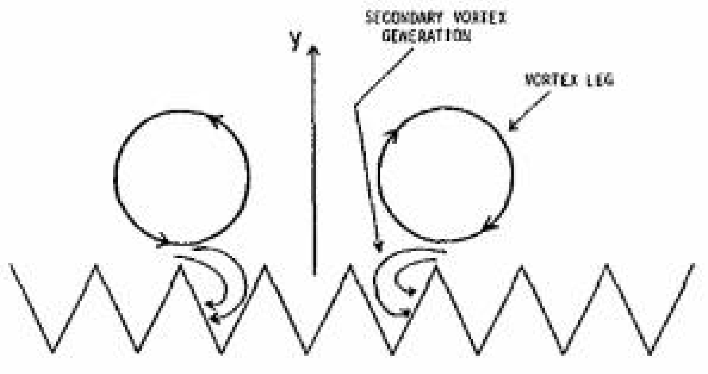
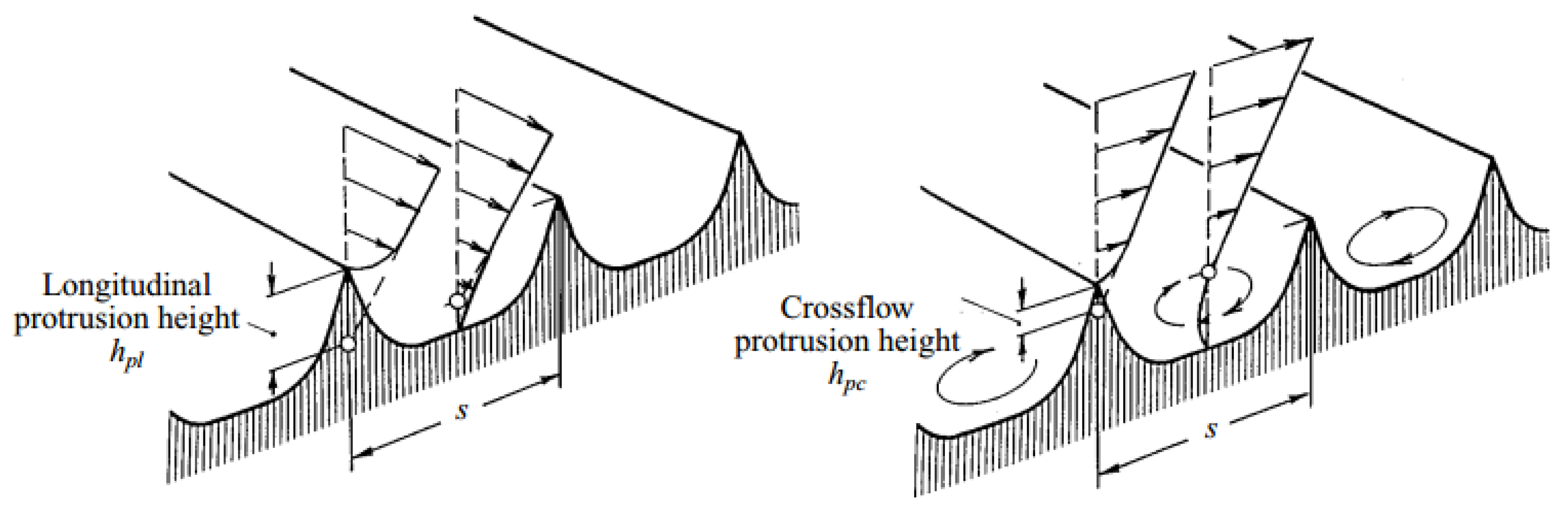
With further advances in experimental and numerical investigations, the microscopic drag reduction mechanism of non-smooth ribletted surfaces has been explored from different perspectives. Generally speaking, discussions of the drag reduction mechanism have diverged into three theories. The “secondary vortex” theory depicts the mechanism from the perspective of a turbulent coherent structure: the secondary vortex is created by the interaction of counter-rotating vortex pairs with the sharp riblet peaks (see Figure 1). The formation and development of the secondary vortex weaken the streamwise vortices related to low-speed streaks, thus dampening the formation and instability of the low-speed streaks. In other words, low-speed streaks raise slowly, the burst is weakened, and the momentum exchange between fluid micelles is decreased, thereby reducing turbulent drag. According to the “protrusion height” theory, from the perspective of viscous wall shear resistance, drag reduction is attained due to an increase in thickness of the viscous sublayer, which decreases the mean gradient of velocity of the wall, consequently decreasing the frictional drag of the wall (see Figure 2). The “air bearing” theory, from the perspective of mechanical drag reduction, proposes the concept of a “micro air bearing system” (MABS) [33]. It is believed that small eddies can set up in the riblet valley and continue swirling (or not swirling), resembling some micro air bearings. The ribletted surfaces thereby gain drag reduction which, according to the principle of rolling friction, is far less than sliding friction. On the other hand, transverse riblets on a flat plate can move the turbulent boundary layer downward. The higher the velocity, the smaller the pressure drop, and consequently, the smaller the friction drag. This is another interpretation of the MABS.
Many researchers have analyzed the drag reduction performance of non-smooth pipes with triangular riblets, drawing the conclusion that drag reduction in a non-smooth pipe is superior to that in a smooth pipe under some conditions. The reason for this phenomenon has been widely researched, with studies mainly focusing on riblets of the same size, with few studies investigating riblets of varying dimensions. Additionally, multi-dimensional studies including mean streamwise velocity, velocity fluctuations, Reynolds shear stress, and Y-vorticity have not been adopted in these analyses and further research is necessary. In the present study, we conjecture about a new form of riblet geometry and whether better drag reduction performance can be achieved if a smaller riblet is added into the space between two riblets and whether high-speed flow is pushed outside the riblets.
2. Materials and Methods
In this study, an LES method was used in a fully turbulent pipe flow. The governing equations employed for LES are obtained by filtering the time-dependent Navier-Stokes equations. To separate large-scale and small-scale motion, a filtering operation is defined to decompose the velocity into the sum of a filtered (or resolved, or large-scale) component and a residual (or subgrid-scale (SGS)) component [35]. In LES, large-scale turbulent motions are directly resolved while small-scale motions are modelled to constrain the closure of the Reynolds equations.
The filtering operation is defined with volume-finite discretization by
where integration is over the volume of a computational cell, . The filter function is
The filtered momentum and continuity equations are
where is the density, is the time, is the filtered component of velocity, µ is the dynamic viscosity, and is the pressure; is the unsolved subgrid-scale stress tensor.
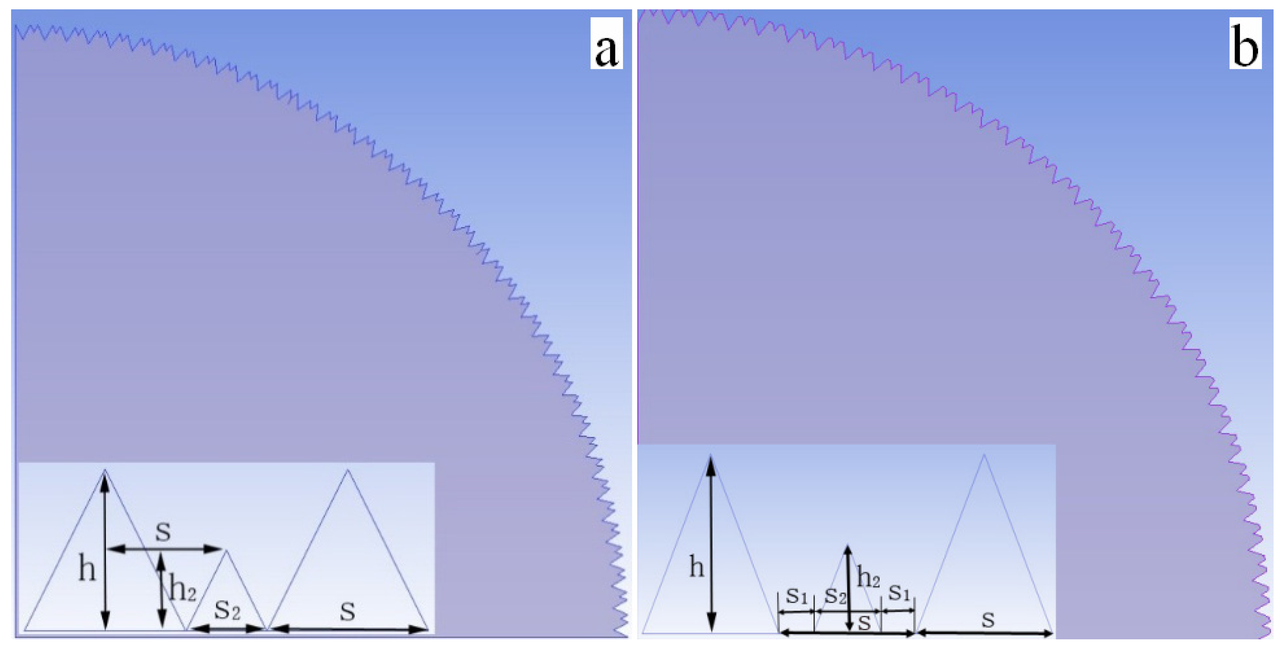
Subgrid-scale models, such as the Smagorinsky eddy viscosity model, Germano dynamic model, scale-similar model, and structural function model, are commonly used in LES. The eddy viscosity model first proposed by Smagorinsky [36] was adopted here and is the mostly commonly used. The friction-reducing shark skin effect on the surface of a pipe results in lower energy consumption. Reduced friction in the flow of the pipe also leads to higher efficiency. Therefore, pipe surfaces would benefit from a riblet structure similar to the riblets on shark scales. As shown in Figure 3, dermal denticles (skin teeth) are shaped like small riblets. The size, length, and height of the ridge structure on shark scales vary and the ridges are aligned in the direction of the fluid flow. Riblets used in previous research have been two dimensional, such that the shape and size of a single riblet remained unchanged in the flow direction. Drawing inspiration from shark scales, we designed two biomimetic topologies of riblets in a non-smooth pipe, as shown in Figure 4. The main characteristics of the C1 and C2 riblets used in this research are provided in Table 1.
The common practice when performing LES of turbulent pipe flow is to create two pipe models, one with a smooth surface and the other with a non-smooth surface. The effective diameter of the non-smooth pipe, which is directly related to the Reynolds number and frictional drag of the turbulent pipe flow, can be calculated from the cross-sectional area of the non-smooth pipe [37]:
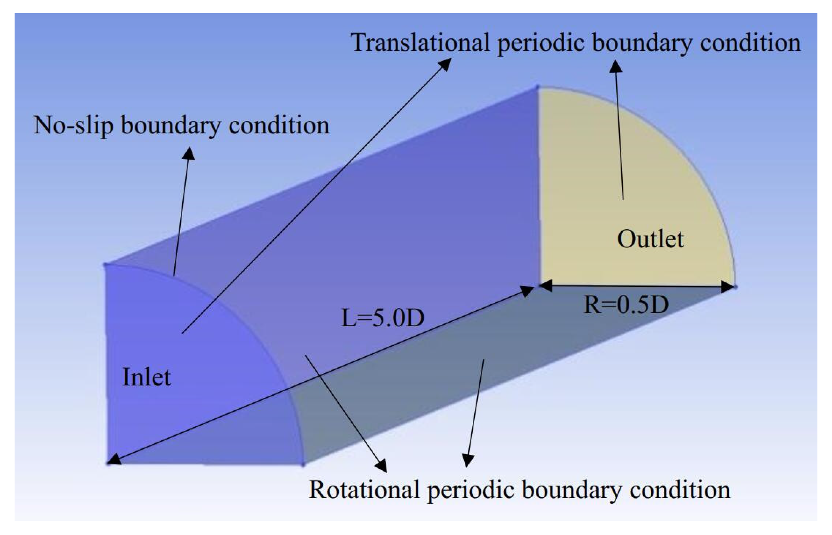
The length and diameter of the non-smooth pipe should be coordinated to eliminate the influence of the flow inlet, thus ensuring that the turbulent flow in the tested section is fully developed. According to the suggestion by Eggels [38], the length here was L = 5D. The length of the smooth pipe was equal to that of the non-smooth pipe, and its diameter was equal to the effective diameter of the non-smooth pipe, DSMOOTH = dr.
As pipe flow has periodical axial symmetry, we took one quarter of the pipe to represent the whole pipe in numerical simulation. To ensure that the flow field in one quarter of the pipe was highly similar to that in reality, a rotational periodic boundary condition was applied in the two spanwise sections and a translational periodic boundary condition was applied in the inlet and outlet. The usual no-slip boundary condition was applied on the wall of both the smooth and non-smooth pipes. A schematic diagram of the computational domains and boundary conditions is shown in Figure 5.
The desired Reynolds number is obtained by imposing a steady mass flow condition. According to:
Then bulk velocity:
Therefore, mass flow rate:
A steady mass flow condition is obtained by setting the mass flow rate. The values of parameters related to Equations (7)–(9) are shown in Table 2.
To ensure the precision, stability, and efficiency of the calculations in this research, several points need particular attention in meshing when using LES. First, mesh refinement near the wall is necessary in the radial direction to ensure sufficient cells in the boundary layer and riblet valleys; thus, the first grid point near the wall is located at y+ ≈ 1 according to previous experience and the requirements of LES [39]. Second, mesh coarsening away from the pipe wall helps to reduce the overall number of cells. Third, streamwise and spanwise meshing should be uniformly distributed. Fourth, the cell size should be small enough to capture the coherent structure and other flow features. Last, but not least, the meshing of the non-smooth pipe with riblets and the smooth pipe should be basically the same. An appropriate time step strongly influences accuracy and time expenditure. According to the suggestion by Wu and Moin [40], the time step should be relatively small at the beginning of the calculation to eliminate the “priming effect” caused by an initial velocity field that does not fit with reality. The time step can be appropriately increased after a period of calculation time. In the first 500 iterations, the maximum axial CFL component was fixed at a small value of 0.05 and the corresponding time step Δt was approximately 0.0002. This was to allow the start-up effect associated with the imposed unrealistic initial velocity field to diminish. After the first 500 iterations, the computational time step was fixed at Δt = 0.01 and the maximum allowed axial CFL component was set at 1.0.
The irregularity and transience of turbulence make it difficult to perfectly initialize the turbulent flow field; we can merely set up an approximate initial condition. Here, we applied translational periodic boundary conditions on the inlet and outlet, which will ensure that the turbulence in the pipe is fully developed, and we shortened the computational length to 5/2π times the diameter of the pipe. We imposed a steady mass flow condition and pressure gradient to drive the flow, and initialized the flow field with laminar flow. Although it does not affect the computational result, appropriate setting of the pressure gradient can accelerate the convergence speed and minimize the calculation time. Statistical sampling should not begin until the numerical computation is convergent, with the effects of the initial and boundary conditions eliminated, indicating that the flow field has reached statistical equilibrium and is infinitely similar to the “real” developed turbulence due to time averaging and the transiency of turbulence. This normally requires more than 10,000 numerical iterations. There are several rules for determining convergence. It is meaningless to monitoring residuals because of the unsteady model we adopted in LES. Several flow statistics should be monitored, such as drag and wall shear stress, and convergence is acheieved when these statistics are steady or fluctuate within a certain range. Sufficient time steps should be continued after convergence, and we applied time averaging to the data recorded during this period. The time required to determine an average is normally twice that taken by the mean flow to traverse the computational domain [41]. Only after these procedures are the data rational and correct.
3. Results and Discussion
The mechanism of turbulent drag reduction over the shark skin-inspired riblets is analyzed and discussed as follows: we investigate the turbulent flow field of the non-smooth pipe with new biomimetic riblets and analyze in detail the evolution of a coherent structure near the wall, drag reduction performance, and the underlying mechanism.
3.1. Evolution of a Coherent Structure near the Wall
The discovery of a coherent structure in pipe turbulence played an important role in this research. In this study, we revealed the evolution of a coherent structure near the wall in the smooth pipe and verified that the pre-processing of the pipe flow field was correct and rational by showing that we were able to capture and quantify the most important flow features.
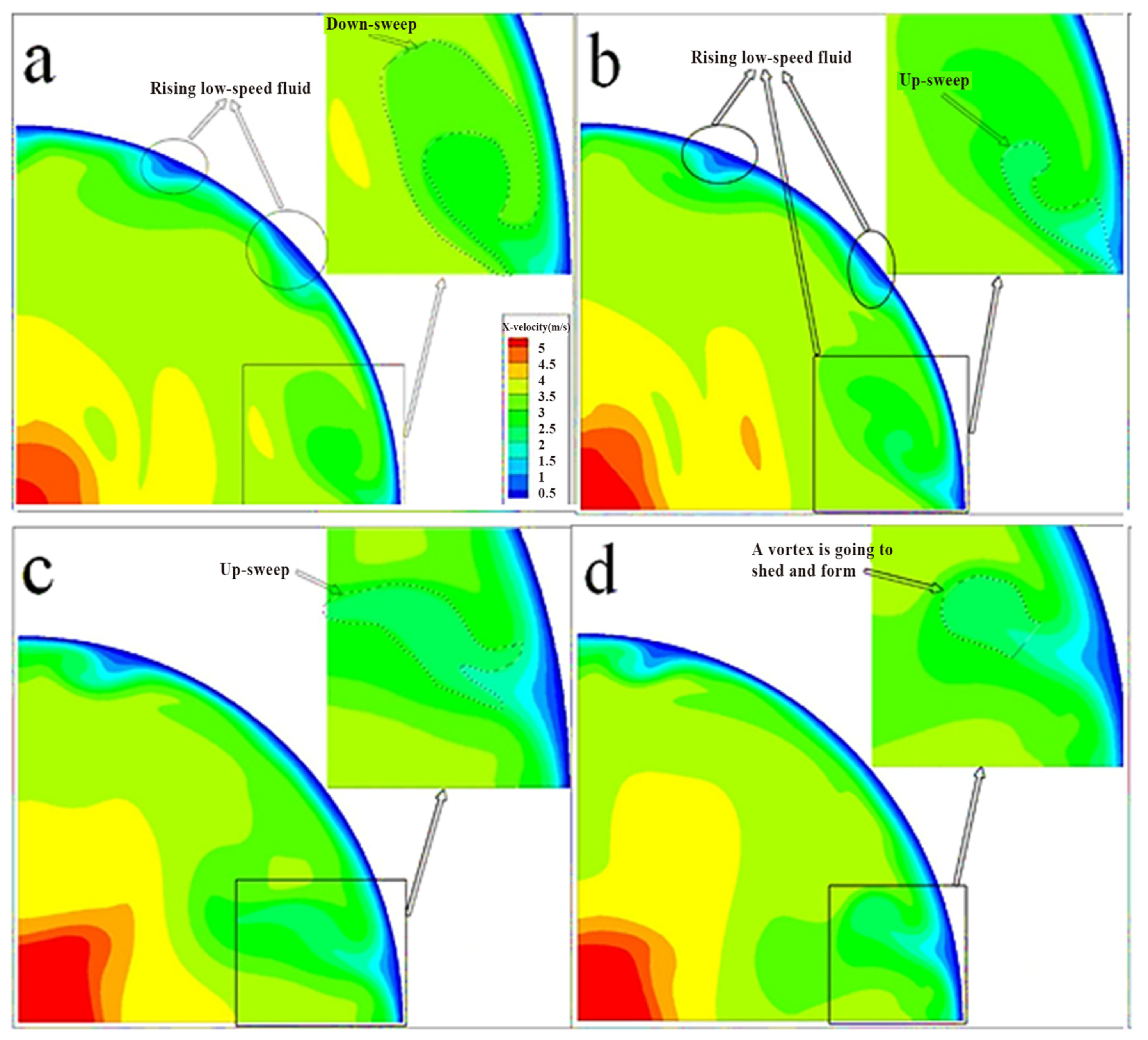
Figure 6 was obtained by monitoring the streamwise velocity of the same cross-section in four consecutive flow periods (Figure 6a–d). This figure provides a concrete description of the evolution of a coherent structure near the pipe wall: the blue area in the images represents low-speed fluid near the wall. As seen in Figure 6a, there are two areas of rising fluid (marked by circles) and one down-sweep event (marked by a dotted line), which is formed after the bursting of streaks in a previous bursting period. In Figure 6b, new low-speed fluid has appeared in the box in the lower right corner due to the down-sweep event. A new up-sweep event (marked by a dotted line) is clearly seen in the magnified view in the upper right corner. Compared with Figure 6b, the height of the low-speed streaks is increasing in Figure 6c, intense oscillation occurs, and the shape of the up-sweep flow (marked by a dotted line) undergoes a rapid change. In Figure 6d, the bursting process has reached the final stage, the low-speed streak is about to burst, and a vortex will shed and form (marked by a dotted line) in the magnified view in upper right corner. Once the streak bursts, the intense turbulent fluctuation forces the flow to accelerate in the streamwise direction and be directed towards the wall, resulting in the down-sweep event mentioned above. This describes the complete process of the coherent structure. After a certain time interval, which is random and varies in length due to the irregularity of turbulence, the down-sweep event affects the near-wall flow again, triggering the formation and rise of new low-speed streaks. The bursting period of the coherent structure of the flow field is obtained by averaging a large amount of data in that time interval.
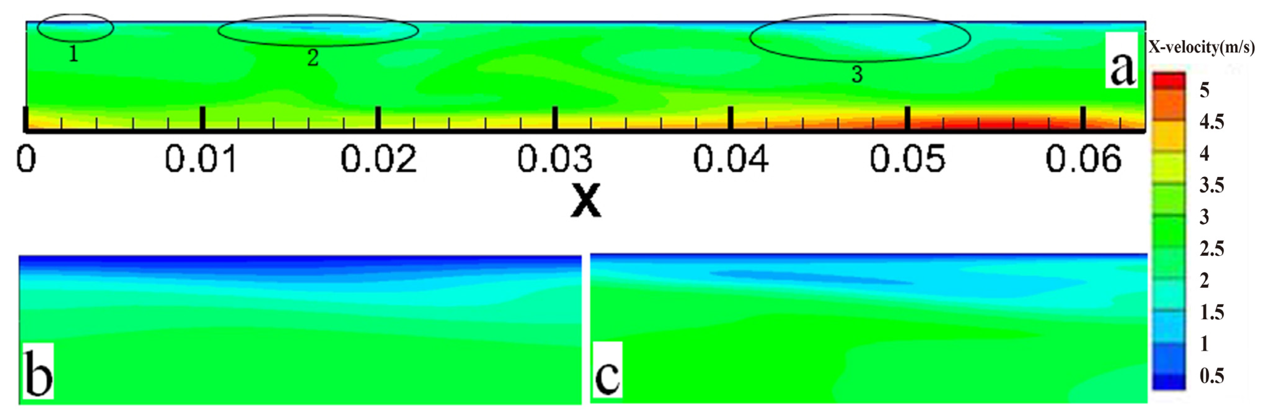
Figure 7a shows the coherent structure observed in the section parallel to the streamwise direction. Low-speed streaks occur in the near-wall region in non-continuous form. Zoomed in regions marked by ellipses 1 and 2 are shown in Figure 7b,c, respectively. The streak in ellipse 1 is just beginning to rise, whereas that in ellipse 2 has reached a greater height. The front part of the streak rises slowly with the movement downstream, along with time averaging flow. The streak is stretched due to the shear stress produced by contact with the outer flow moving at a greater speed. Vortices form and shed, showing that the bursting process of the coherent structure is complete.
3.2. Turbulent Drag
The turbulent drag of smooth and non-smooth pipes with riblets C1 and C2 at different Re numbers is listed in Table 3. As can be seen, the friction drag of non-smooth pipes with either riblet C1 or C2 is, in all cases, less than that of the smooth pipe, indicating that the two new biomimetic non-smooth pipe surfaces produced good drag reduction performance in turbulent pipe flow. The amount of drag reduction was significantly increased when a small riblet was added between two contiguous riblets, as in the non-smooth pipe with riblets C1 and C2. The distance between the riblets did not offset the drag reduction effect resulting from the presence of small riblets. The drag reduction effect of the non-smooth pipe with riblet C2 was clearly superior to that with riblet C1, with the maximum drag reduction gained with riblet C2 at Re = 40,459 (s+ = 18.9737). We can state that the optimum drag reduction s+ was not less than 18.9737, but we could determine the exact value. With reference to formerly published research, we next studied the turbulent drag of the two biomimetic topologies using riblets C1 and C2, in comparison with the results shown in Table 4. The ribletted pipes studied in the present work showed excellent drag reduction performance. Riblet C2, designed from the bionic perspective, evidenced the best drag reduction performance in this research.
3.3. Thickness of Viscous Sublayer
The turbulent motion in the pipeline is generally divided into three areas with different properties (core area of turbulence, viscous bottom region, and transition area), which can be divided according to the following formula:
When , this region is the viscous bottom layer.
When , this region is the transition region.
When , this region is the core region of turbulence.
Thus, an empirical formula for the thickness of the viscous bottom layer can be obtained as follows: . Where y is the distance from the pipe wall, ν is coefficient of kinematical viscosity, the friction velocity is defined by , τw is the wall shear stress, and ρ is the density of the fluid.
As shown in Table 5, the thickness of a viscous sublayer in non-smooth pipes with riblets C1 and C2, which proved to reduce drag, was greater than that of the smooth pipe. The greater the drag reduction, the greater the increase in thickness of the viscous sublayer. This result fully vindicated the claim that increasing the thickness of the viscous sublayer greatly influences the drag reduction performance and that the lubricant effect is one aspect of the drag reduction mechanisms. The presence of riblets increased the thickness of the viscous sublayer and steadied the flow in the boundary layer of the non-smooth pipes. On the other hand, the flow in the viscous sublayer acted like lubricant that significantly decreased the frictional drag between the high-speed outer flow and the ribletted surfaces.
3.4. Analysis of Turbulent Flow Field
Multi-dimensional data of mean streamwise velocity profiles, velocity fluctuations, Reynolds shear stress, and vorticity distributions between smooth and non-smooth pipes with riblets C1 and C2 at Re = 40,459 were compared to illustrate the drag reduction mechanisms.
3.4.1. Velocity Profiles
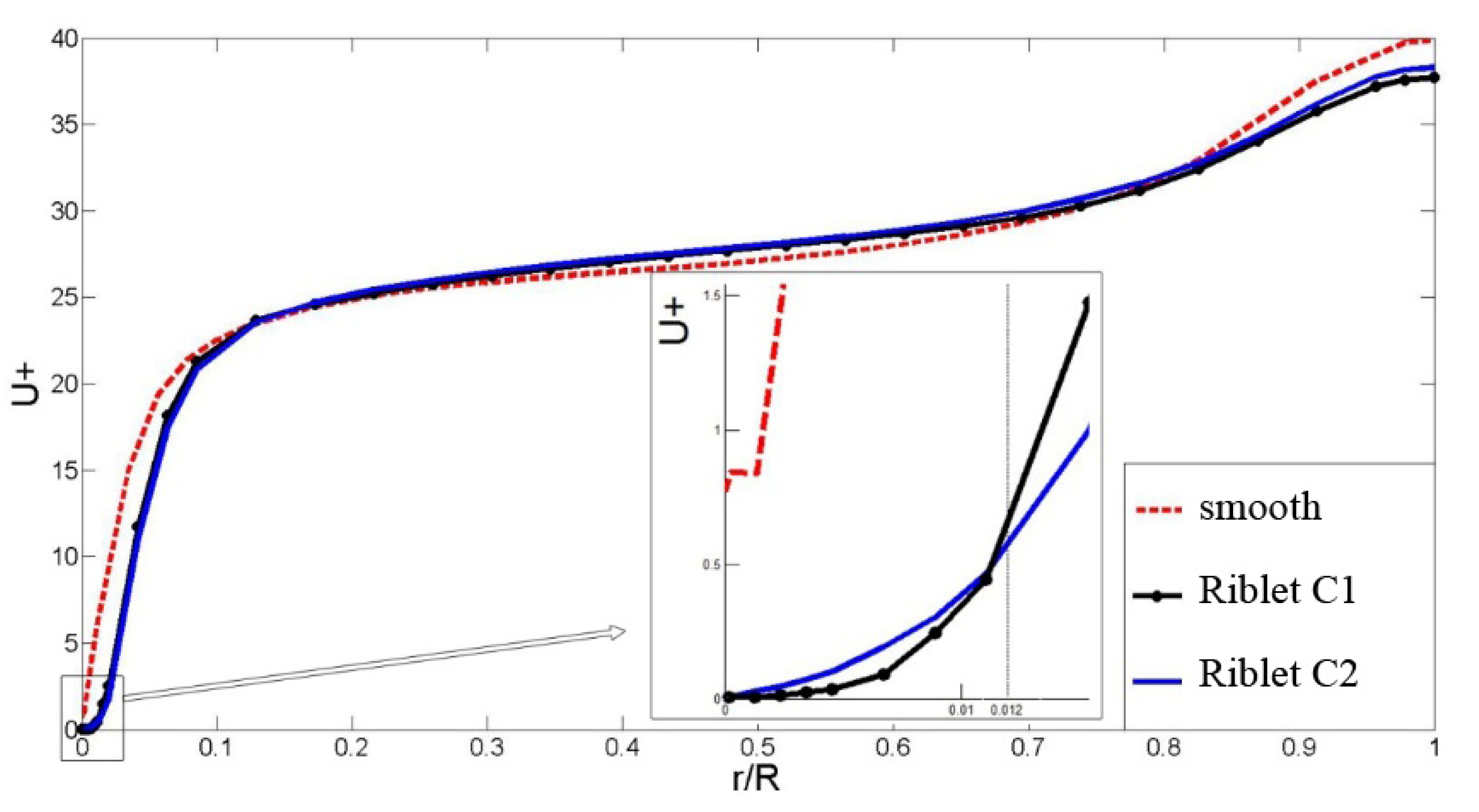
Figure 8 shows the mean streamwise velocity profiles of the smooth and non-smooth pipes over riblet valleys. The streamwise velocity in riblet valleys where (r is the distance away from the pipe wall and R is the radius of the pipe) was very low, indicating that the flow in riblet valleys was smooth and slow. There is an obvious demarcation point near the region of , at which point the two curves of the non-smooth pipes with riblets C1 and C2 intersected. Below this point in the curves, the mean flow velocity of the non-smooth pipe with riblet C2 had higher values. Affected by the riblets, the mean velocities in the region of the non-smooth pipes with riblets C1 and C2 were lower than that of the smooth pipe. These findings illustrated that the non-smooth pipes with riblets C1 and C2 showed good drag reduction performance. The two curves almost coincided at .
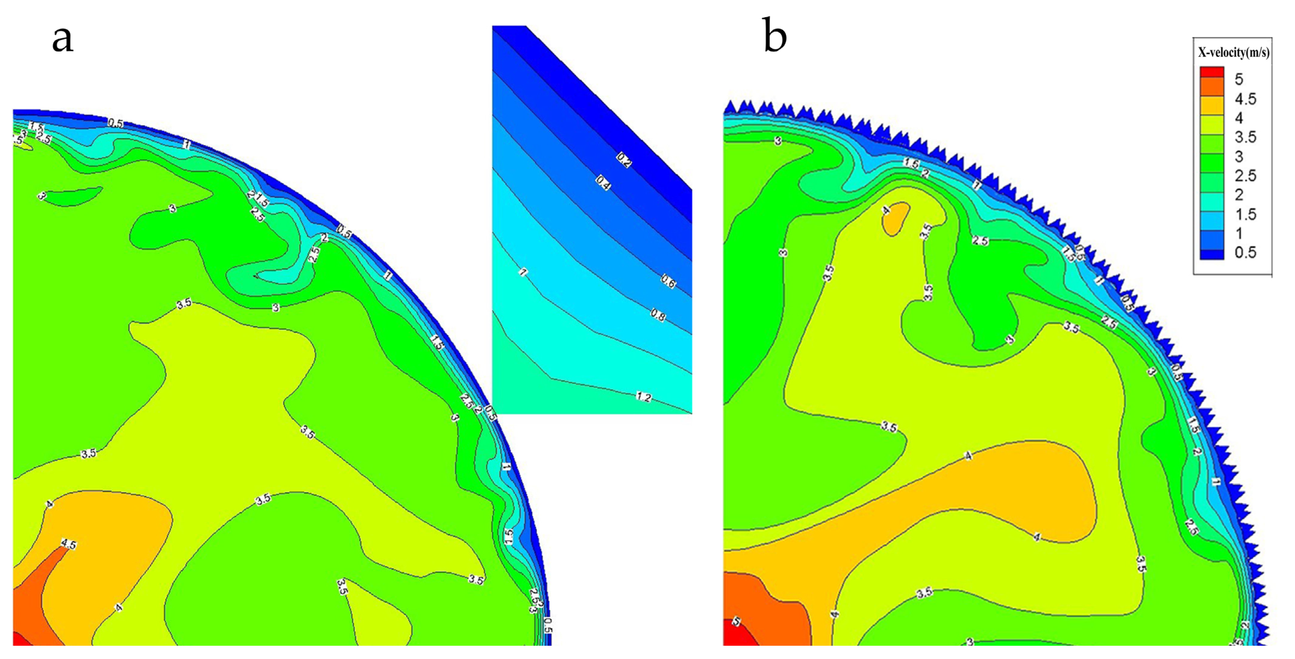
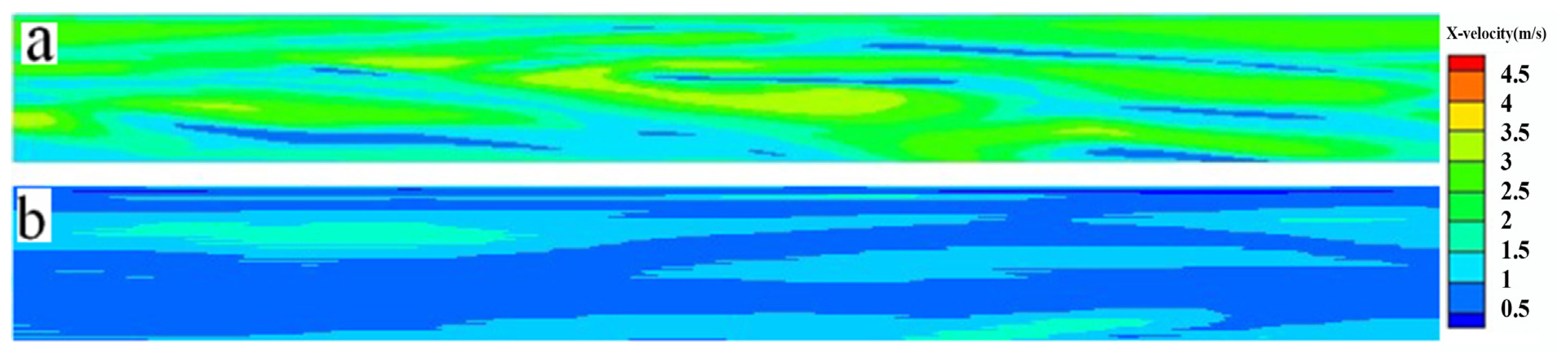
Clearly, the velocities in the near-wall region of the smooth pipe were higher than those of the non-smooth pipes, when comparisons were made between the contours of the streamwise velocity of the smooth pipe and the non-smooth pipe with riblet C1 at Re = 40,459 in a section perpendicular to the flow direction (Figure 9) and in a near-wall region where (Figure 10, blue contours indicate low-speed flow). The velocity of the flow in riblet valleys and in a certain region outside the riblet tips was lower than that of the outer flow, as can be seen in the contours of Figure 9. In general, low-speed flow in the near-wall region of the non-smooth pipe with riblet C1 is demonstrated, illustrating that high-speed flow traverses the pipe on top of the low-speed flow, avoiding energy dissipation due to direct pipe wall contact, and the friction drag is consequently reduced. The presence of low-speed flow also maintains the stability of the boundary layer and helps dampen the turbulence to avoid bursting.
3.4.2. Velocity Fluctuation
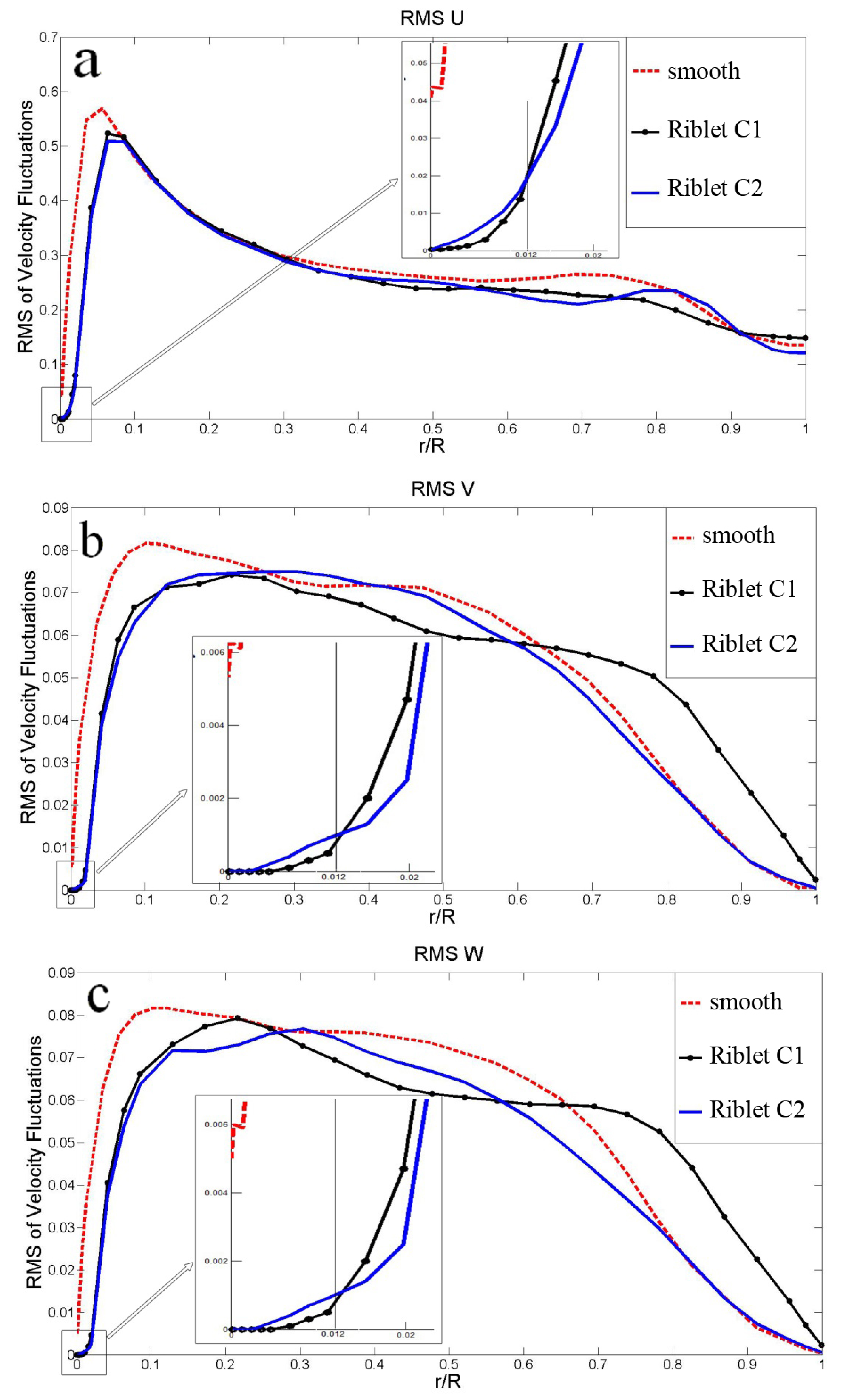
Figure 11 compares the root-mean-square (RMS) values in U, V, and W directions of the smooth and non-smooth pipes over riblet valleys at Re = 40,459. Figure 12 shows the contours of the RMS values of velocity at the vertical flow cross-section. Figure 13 shows the contours of RMS values of velocity magnitude of a non-smooth pipe with riblet C1 at Re = 40,459 in the near-wall region where . Figure 11 reveals that the RMS values in the three directions of the smooth pipe were higher than those of the non-smooth pipe in the region where at Re = 40,459, and the greater the drag, the higher the RMS values of velocity fluctuations. One aspect was commonly observed in the comparison of velocity fluctuations in three directions of the non-smooth pipes with riblets C1 and C2 in Figure 11: when , the RMS values of the velocity fluctuations of the non-smooth pipe with riblet C2 in the three directions were higher than those of the non-smooth pipe with riblet C1 in the riblet valley where . The velocity fluctuations in the near-wall region were reduced by the triangular riblets and turbulent bursting was dampened, matching perfectly with the observations of Choi [44] and Wu et al. [43], in which the velocity fluctuations of all components in a drag-reducing configuration decreased above the riblets.
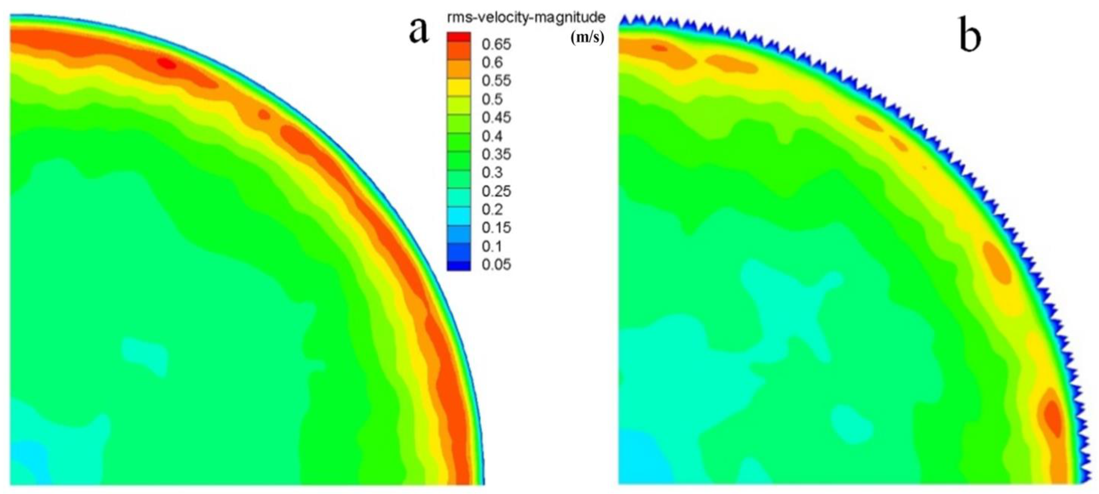
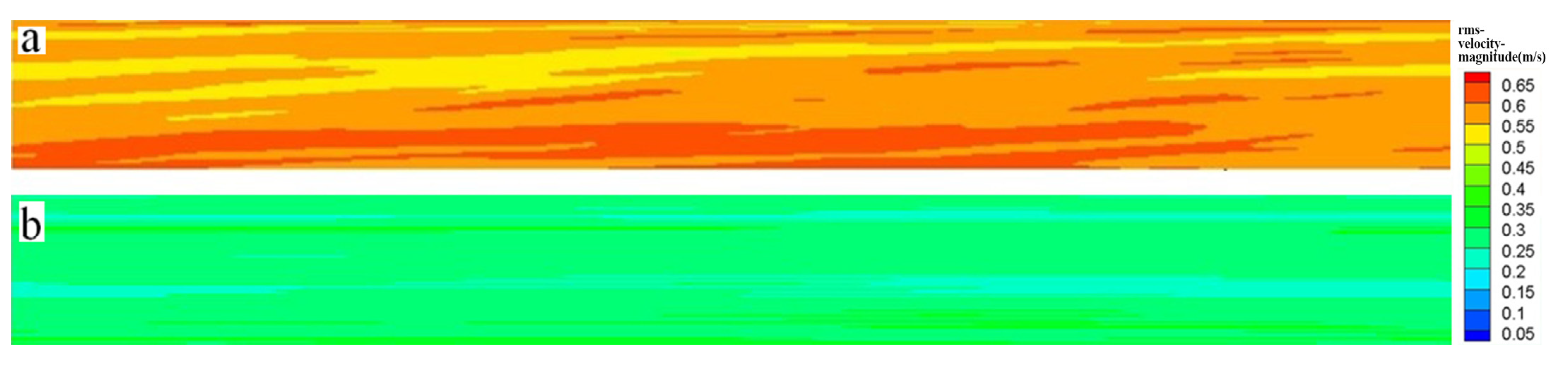
Figure 12 and Figure 13 clearly show that the non-smooth pipe with riblet C1 had an obvious inhibitory effect on velocity fluctuations in the near-wall region of the pipe. As shown in Figure 12a, the velocity fluctuations of the smooth pipe were more intense near the wall, forming a red circle. Different phenomena are observed in Figure 12b, where under the influence of riblets, the red circle is scattered, and its thickness is reduced. The contours of velocity fluctuations in the near-wall region of pipes are shown in Figure 13. Obviously, the velocity fluctuations of the non-smooth pipe with riblet C1 were much lower than that of the smooth pipe in the region of .
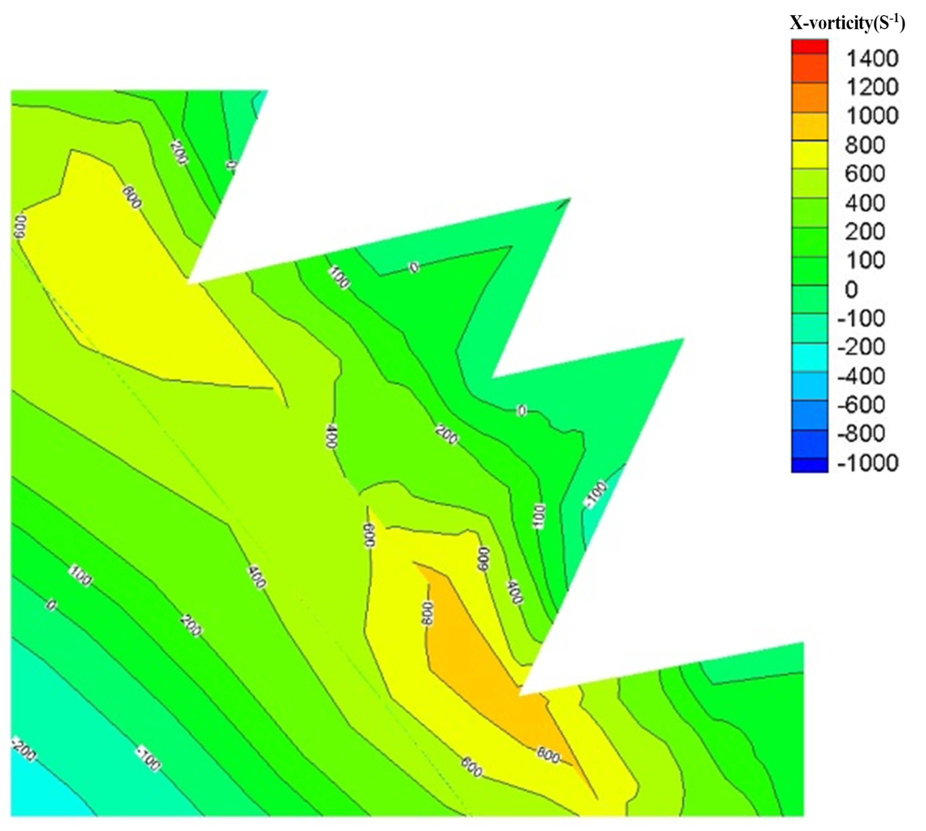
3.4.3. Streamwise Vorticity Distribution
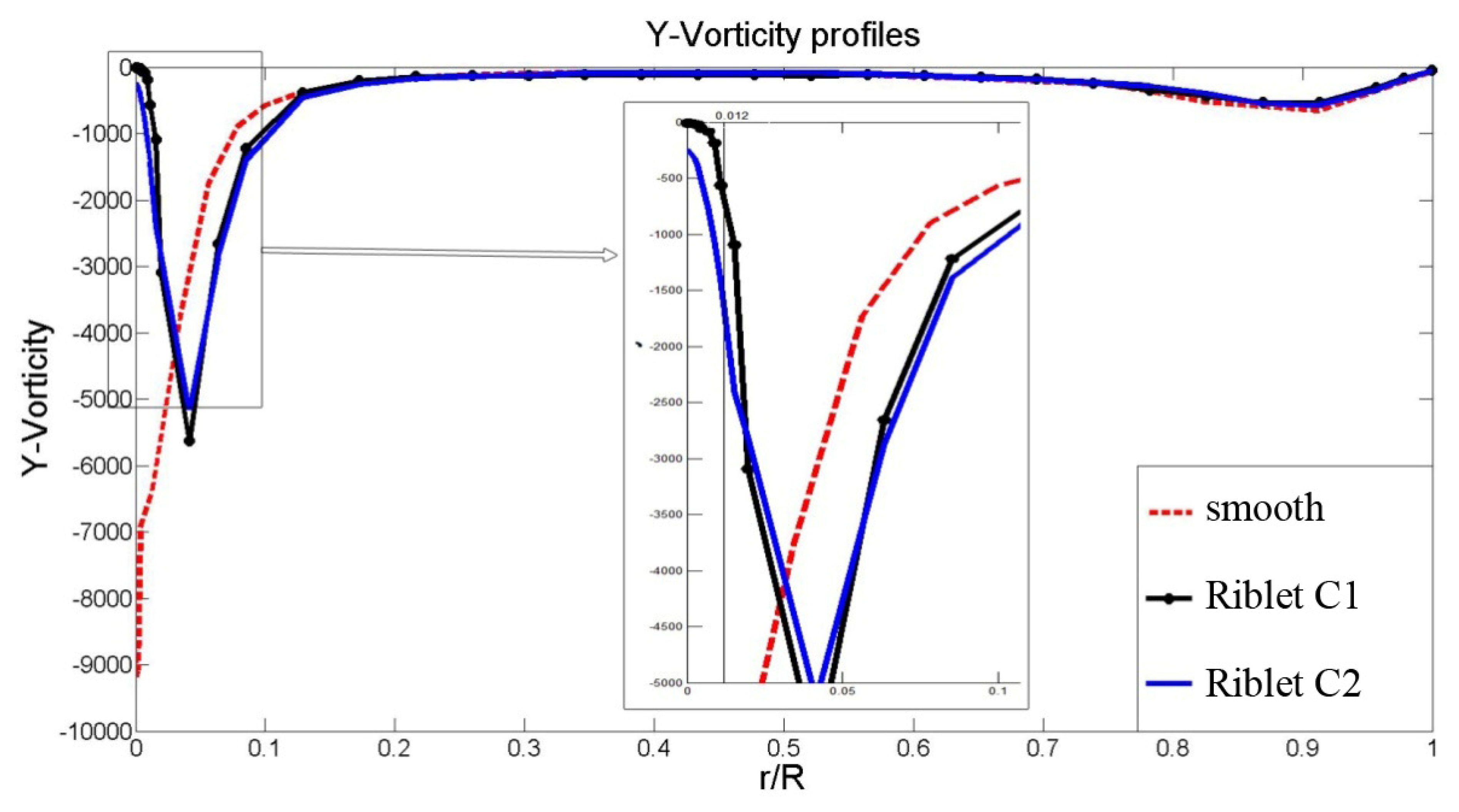
Figure 14 shows the contours of vorticity in the X direction of a non-smooth pipe with riblet C1 at Re = 40,459. It is interesting that there are secondary vortices adhering to the tips of the large riblets, but no vortices adhering to the tips of the small riblets, and the vorticity value equals zero in the region of . In other words, small riblets pushed out vortices between two big riblets, minimizing disturbance in the region of the riblets and finally maintaining flow stability in the pipe. These findings show the beneficial effect of drag reduction. Figure 15 compares the Y-vorticity of smooth and non-smooth pipes with riblets C1 and C2 at Re = 40,459. The Y-vorticity of the smooth pipe was higher than that of the non-smooth pipes where (riblet valley), and the greater the turbulent drag, the higher the Y-vorticity. Figure 15 shows that more lateral vortices entered the riblet C1 valley, partly weakening the ability of the riblets to impede lateral vorticity. Consequently, the drag reduction performance of riblet C2 was superior to that of riblet C1. Distribution of vorticity in the Y direction was limited to the near-surface region of the pipe, and the decrease of vorticity in this small area stabilized the flow of the boundary layer and inhibited turbulence in this area from bursting.
According to the analysis presented here, riblets had a sheltering effect on cross flow and lateral vorticity, which was consistent with Luchini’s findings [13]. Research has focused on streamwise velocity and vortices because of their dominant role in the flow field. However, we found that it is also important to pay attention to cross flow, such as tangential velocity, Y-vorticity, and Z-vorticity, by recognizing the differences between smooth and non-smooth pipes.
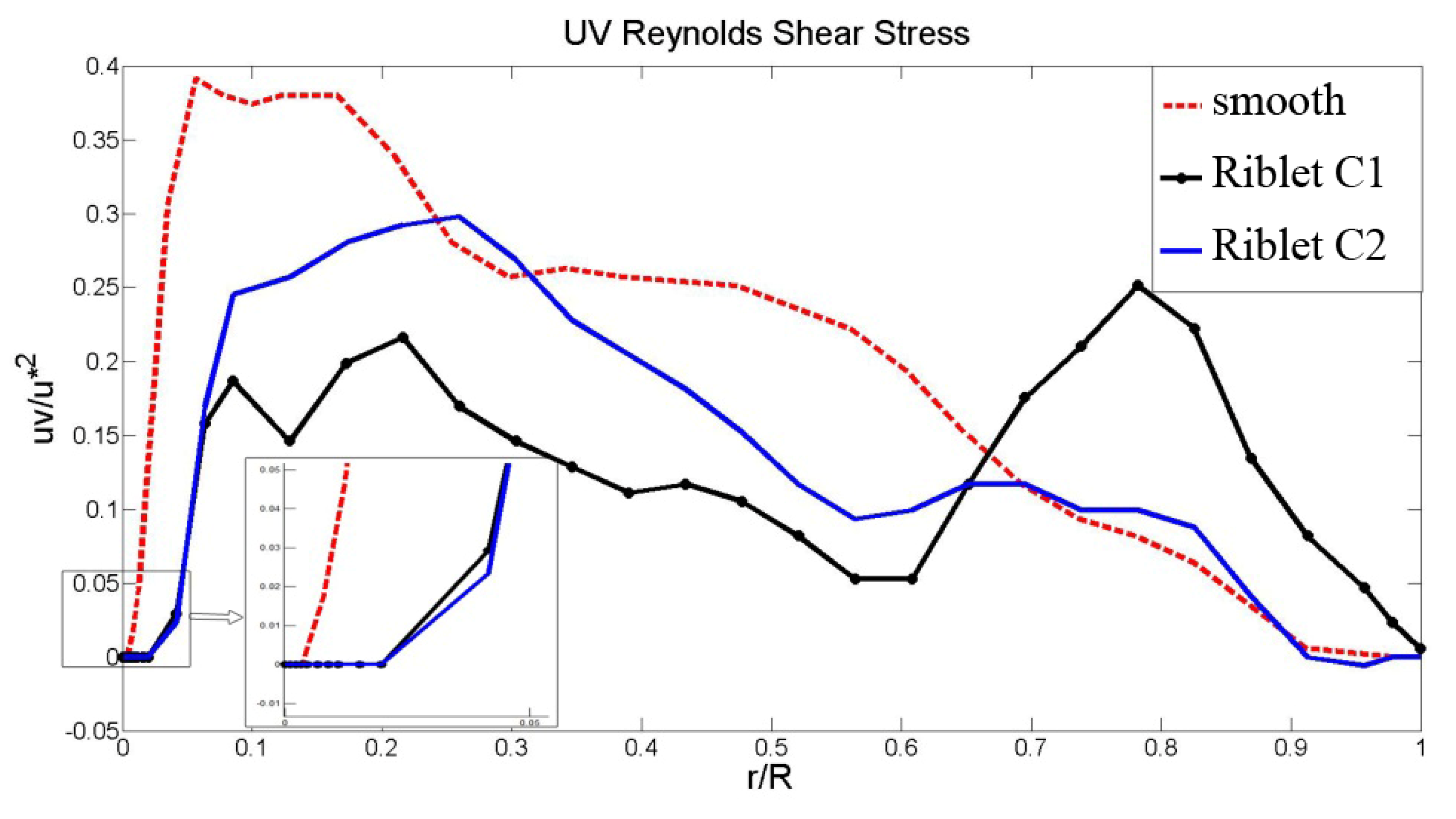
3.4.4. Reynolds Shear Stress
Figure 16 shows a comparison of the UV Reynolds shear stress of smooth and non-smooth pipes at Re = 40,459. Some different phenomena were observed at the point . Under this point of the curves, the Reynolds shear stress of the non-smooth pipe with riblet C1 had higher values. The non-smooth pipe with riblet C2, with a shape similar to the biological prototype of shark scales, showed the best drag reduction performance, and the thickness of the viscous layer was increased while the streamwise velocity, velocity fluctuation, Reynolds shear stress, and lateral vorticity were decreased due to interaction between the riblets and turbulent flow in the pipes. An obvious demarcation point near the region of was at the top of the small riblets. Below this point in the curves, the mean flow velocity, velocity fluctuation, and Y-vorticity of the non-smooth pipe with riblet C2 had higher values. In contrast, the values of the non-smooth pipe with riblet C2 were lower than those of the non-smooth pipe with riblet C1. The reason is very clear: the greater high-speed flow and vorticity found in the region of the riblets due to the increased distance between riblets of the non-smooth pipe with riblet C2 led to disturbance and increased velocity fluctuation and turbulence intensity. However, the disturbance was limited to a certain region because of the presence of small riblets.
The presence of triangular riblets affected the velocity profile, velocity fluctuations, and Reynolds shear stress in a certain region, i.e., , thereby changing the flow field and increasing drag reduction. For drag reduction over non-smooth surfaces, more attention should be paid to the flow features in the region where .
4. Conclusions
Turbulent flow was simulated over two effective, shark skin-inspired, ribletted pipe surfaces. Drag reduction performance, flow velocity, velocity fluctuation, Reynolds shear stress, and lateral vorticity under different Reynolds numbers were fully illustrated. Riblet C2, which was most similar to the prototype of a shark scale, produced superior drag reduction, showing higher turbulent drag reduction behaviors, e.g., 21.45% at Re = 40,459, compared with other experimental and simulated reports. Numerical simulations supported riblet drag reduction theories from the perspectives of coherent structures, thickness of viscous layer, and secondary vortices. The effects of the riblets on the behavior of fluid flow in pipes were discussed, as well as the mechanisms of fluid drag in turbulent flow and riblet drag reduction. The mechanisms of turbulent drag reduction of ribletted pipes were determined as follows: (1) Riblets impede the translation of streamwise vortices, resulting in a reduction in vortex bursting and outer-layer turbulence. The streamwise velocity of non-smooth pipes was lower than that of a smooth pipe in the near-wall region, and low-speed flow in the riblet valley reduced frictional drag. (2) The thickness of the viscous layer in non-smooth pipes was greater than that of a smooth pipe and the lubricant effect is one aspect of the drag reduction mechanism. (3) The velocity fluctuations in three directions of ribletted pipes were smaller than those of a smooth pipe, indicating that riblets can dampen velocity fluctuations, thereby weakening turbulence intensity of the near-wall region. (4) Riblets can also decrease Reynolds shear stress in the near-wall region, which is also part of the drag reduction mechanisms. (5) Riblets impede transverse turbulent motion, and transverse vorticity plays an important role in keeping the near-wall flows relatively quiescent. We conclude that the better the drag reduction, the greater the thickness of the viscous of sublayer and the lower the mean streamwise velocity, Reynolds shear stress, and transverse vorticity.
Author Contributions
Conceptualization, S.F. and Y.T.; methodology, S.F. and X.H.; software, S.F. and X.H.; validation, S.F., X.H. and Y.T.; formal analysis, S.F. and X.H.; investigation, S.F.; resources, S.F. and X.H.; data curation, Y.W. and X.K.; writing—original draft preparation, S.F.; writing—review and editing, X.H., Y.W. and X.K.; visualization, Y.T.; supervision, X.H.; project administration, X.H.; funding acquisition, X.H. All authors have read and agreed to the published version of the manuscript.
Funding
This research was funded by Beibu Gulf University high-level talents research project (2020KYQD05).
Institutional Review Board Statement
Not applicable.
Informed Consent Statement
Not applicable.
Acknowledgments
The authors would like to thank Runheng Li for his insightful discussion regarding the mechanisms of fluid drag in turbulent flow, riblet drag reduction, and other helpful comments.
Conflicts of Interest
The authors declare no conflict of interest.
Nomenclature
| U | Mean streamwise velocity |
| τw | Wall shear stress |
| u* | Friction velocity |
| U+ | Non-dimensional mean streamwise velocity |
| Non-dimensional riblet spacing | |
| Non-dimensional riblet height | |
| γ | Angle between the flow direction and riblets |
| Cs | Smagorinsky constant |
| D | External diameter of non-smooth pipe |
| A | Cross-sectional area of non-smooth pipe |
| Drag reduction efficiency |
References
- Bechert, D.W.; Bruse, M.; Hage, W. Experiments on drag-reducing surfaces and their optimization with an adjustable geometry. J. Fluid Mech. 1997, 33, 59–87. [Google Scholar] [CrossRef]
- Bechert, D.W.; Bruse, M.; Hage, W. Experiments with three-dimensional riblets as an idealized model of shark skin. Exp. Fluids. 2000, 28, 403–412. [Google Scholar] [CrossRef]
- Bechert, D.W.; Bruse, M.; Hage, W.; Meyer, R. Fluid mechanics of biological surfaces and their technological application. Naturwissenschaften 2000, 87, 157–171. [Google Scholar] [CrossRef] [PubMed]
- Lee, S.J.; Lee, S.H. Flow field analysis of a turbulent boundary layer over a riblet surface. Exp. Fluids 2001, 30, 153–166. [Google Scholar] [CrossRef]
- Djenidi, L.; Antonia, R.A. Laser Doppler anemometer measurements of turbulent boundary layer over a riblet surface. AIAA J. 1996, 34, 1007–1012. [Google Scholar] [CrossRef]
- Rapp, H.; Zoric, I.; Kasemo, B. Microstructured surfaces for drag reduction purposes: Experiments and simulation on rectangular 2D riblets. Mater. Res. Soc. 2006, 899, 808. [Google Scholar] [CrossRef]
- Wang, J.J.; Lan, S.L.; Miao, F.Y. Drag-reduction characteristics of turbulent boundary layer flow over riblets surfaces. Shipbuild. China 2001, 42, 1–5. [Google Scholar]
- Cong, Q.; Feng, Y.; Ren, L.Q. Affecting of riblets shape of nonsmooth surface on drag reduction. J. Hydrodyn. Ser. B 2006, 21, 232–238. [Google Scholar]
- Choi, K.S. Effects of longitudinal pressure gradients on turbulent drag reduction with riblets. In Turbulent Control by Passive Means; Coustols, E., Ed.; Springer: Dordrecht, The Netherlands, 1990; Volume 3, pp. 109–122. [Google Scholar]
- Debisschop, J.P.; Nieuwstadt, T.M. Turbulent boundary layer in an adverse pressure gradient: Effectiveness of riblets. AIAA J. 1996, 34, 932–937. [Google Scholar] [CrossRef]
- Wang, A.W.; Motta, P.; Hidalgo, P.; Westcott, M. Bristled shark skin: A microgeometry for boundary layer control? Bioinsp. Biomim. 2008, 3, 046005. [Google Scholar] [CrossRef] [Green Version]
- Cong, Q.; Feng, Y. Numerical simulation of turbulent flow over triangle riblets. J. Ship Mech. 2006, 10, 11–16. [Google Scholar]
- Luchini, P.; Manzo, F.; Pozzi, A. Resistance of a grooved surface to parallel flow and cross-flow. J. Fluid Mech. 1991, 228, 87–109. [Google Scholar] [CrossRef]
- Fukagata, K. Drag reduction by wavy surfaces. J. Fluid Sci. Technol. 2011, 6, 2–13. [Google Scholar] [CrossRef]
- Nitschke, P. Experimental Investigation of the Turbulent Flow in Smooth and Longitudinal Grooved Pipes Dissertation. Available online: https://ntrs.nasa.gov/api/citations/19880017231/downloads/19880017231.pdf (accessed on 24 October 2014).
- Chen, J.J.J.; Leung, Y.C. Drag reduction in a longitudinally grooved flow channel. Ind. Eng. Chem. Fundam. 1986, 25, 741–745. [Google Scholar] [CrossRef]
- Reidy, L.W.; Anderson, G.W. Drag reduction for external and internal boundary layers using riblets and polymers. In Proceedings of the AIAA 26th Aerospace Sciences Meeting, Reno, NV, USA, 11–14 January 1988. [Google Scholar]
- Enyutin, G.V.; Lashkov, Y.A.; Samoilova, N.V. Drag reduction in riblet-lined pipes. Fluid Dyn. 1995, 30, 45–48. [Google Scholar] [CrossRef]
- Shiki, O.; Takashi, Y.; Masato, K. Drag reduction in pipe flow with riblet. Trans. Jpn. Soc. Mech. Eng. 2002, 68, 1058–1064. [Google Scholar]
- Koeltzsch, K.; Dinkelacker, A.; Grundmann, R. Flow over convergent and divergent wall riblets. Exp. Fluids. 2002, 33, 346–350. [Google Scholar] [CrossRef]
- Auteri, F.; Baron, A.; Belan, M. Campanardi G and Quadrio M Experimental assessment of drag reduction by traveling waves in a turbulent pipe flow. Phys. Fluids 2010, 22, 115103. [Google Scholar] [CrossRef] [Green Version]
- Tang, F.; Yan, Z.L.; Wang, X.H. Experimental research on lift up and drag reduction effect of streamwise travelling wave wall. Key Eng. Mater. 2011, 483, 721–726. [Google Scholar] [CrossRef]
- Ahn, J.; Choi, H.; Lee, J.S. Large eddy simulation of flow and heat transfer in a channel roughened by square or semicircle ribs. J. Turbomach. 2005, 127, 263–269. [Google Scholar] [CrossRef]
- Peet, Y.; Sagaut, P. Turbulent drag reduction using sinusoidal riblets with triangular cross-section. In Proceedings of the 38th AIAA Fluid Dynamics Conference and Exhibit, Seattle, WA, USA, 23–26 June 2008. [Google Scholar]
- Martin, S.; Bhushan, B. Fluid flow analysis of continuous and segmented riblet structures. Rsc. Adv. 2016, 6, 10962–10978. [Google Scholar] [CrossRef]
- Martin, S.; Bhushan, B. Modeling and optimization of shark-inspired riblet geometries for low drag applications. J. Colloid Interface Sci. 2016, 474, 206–215. [Google Scholar] [CrossRef] [PubMed]
- Ibrahim, M.D.; Amran, S.N.A.; Yunos, Y.S.; Ramham, M.R.A.; Mohtar, M.Z.; Wong, L.K.; Zulakharmain, A. The study of drag reduction on ships inspired by simplified shark skin imitation. Appl. Bionics Biomechan. 2018, 2018, 7854321. [Google Scholar] [CrossRef] [PubMed] [Green Version]
- Du Clos, K.T.; Lang, A.; Devey, S.; Motta, P.J.; Habegger, M.L.; Gemmell, B.J. Passive bristling of mako shark scales in reversing flows. J. R. Soc. Interface 2018, 15, 20180473. [Google Scholar] [CrossRef]
- Lloyd, C.J.; Peakall, J.; Burns, A.D.; Keevil, G.M.; Dorrell, R.M.; Wignall, P.B.; Fletcher, T.M. Hydrodynamic efficiency in sharks: The combined role of riblets and denticles. Bioinspir. Biomim. 2021, 16. [Google Scholar] [CrossRef]
- Genc, M.S.; Kemal, K.; Acikel, H.H. Investigation of pre-stall flow control on wind turbine blade airfoil using roughness element. Energy 2019, 176, 320–334. [Google Scholar] [CrossRef]
- Koca, K.; Genç, M.S.; Özkan, R. Mapping of laminar separation bubble and bubble-induced vibrations over a turbine blade at low Reynolds numbers. Ocean Eng. 2021, 239. [Google Scholar] [CrossRef]
- Koca, K.; Genç, M.S.; Veerasamy, D.; Özden, M. Experimental flow control investigation over suction surface of turbine blade with local surface passive oscillation. Ocean Eng. 2022, 266, 113024. [Google Scholar] [CrossRef]
- Pan, J. The experimental approach to drag reduction of the transverse ribbons on turbulent flow. ACTA Aerodyn. Sin. 1996, 14, 304–310. [Google Scholar]
- Bacher, E.V.; Smith, C.R. A combined visualization-anemometry study of the turbulent drag reducing mechanisms of triangular micro-groove surface modifications. In Proceedings of the AIAA Shear Flow Control Conference, Boulder, CO, USA, 12–14 March 1985. [Google Scholar]
- Schumann, U. Subgrid scale model for finite difference simulations of turbulent flows in plane channels and annuli. J. Comput. Phys. 1975, 18, 376–404. [Google Scholar] [CrossRef] [Green Version]
- Smagorinsky, J. General circulation experiments with the primitive equations. I. The basic experiment. Mon. Weather Rev. 1963, 91, 99–164. [Google Scholar] [CrossRef]
- Liu, K.N.; Christodoulou, C.; Riccius, O.; Joseph, D.D. Drag reduction in pipes lined with riblets. AIAA 1990, 28, 1697–1698. [Google Scholar] [CrossRef]
- Byun, D. Drag reduction on micro-structured super-hydrophobic surface. IEEE Int. Conf. Robot. Biomim. 2006, 818–823. [Google Scholar] [CrossRef]
- Wu, N. Study on Turbulent Drag Characteristics of Non-Smooth Surfaces Using Large Eddy Simulation MEng Dissertation. Master’s Thesis, South China University of Technology, Guangzhou, China, 1 June 2012. (In Chinese). [Google Scholar]
- Wu, X.H.; Moin, P. A direct numerical simulation study on the mean velocity characteristics in turbulent pipe flow. J. Fluid Mech. 2008, 608, 81–112. [Google Scholar] [CrossRef]
- Vijiapurapu, S.; Cui, J. Large eddy simulation of fully developed turbulent pipe flow. In Proceedings of the ASME Heat Transfer/Fluids Engineering Summer Conference, Charlotte, NC, USA, 11–15 July 2004. [Google Scholar]
- Zhang, D.Y.; Luo, Y.H.; Li, X.; Chen, H.W. Numerical simulation and experimental study of drag reducing surface of a real shark skin. J. Hydrodyn. 2011, 23, 204–211. [Google Scholar] [CrossRef]
- Wu, N.; Tang, Y.; Zhao, C.; Lin, W.; Chen, X.; Li, R. Numerical investigation of a blade riblet surface for drag reduction applications with large eddy simulation method. Appl. Mech. Mater. 2012, 187, 315–319. [Google Scholar] [CrossRef]
- Choi, H.; Moin, P.; Kim, J. Direct numerical simulation of turbulent flow over riblets. J. Fluid Mech. 1993, 255, 503. [Google Scholar] [CrossRef]
Figure 1.
Schematic demonstration of streamwise vortex interaction with ribletted surface via viscous effects [34].
Figure 1.
Schematic demonstration of streamwise vortex interaction with ribletted surface via viscous effects [34].

Figure 2.
Schematic of mean velocity profiles and effective protrusion heights for flow in both the longitudinal protrusion direction, hpl, and cross-flow direction, hpc [1].
Figure 2.
Schematic of mean velocity profiles and effective protrusion heights for flow in both the longitudinal protrusion direction, hpl, and cross-flow direction, hpc [1].

Figure 3.
Diagram of shark scales.

Figure 4.
Diagram of cross-section of pipes with riblets (a) C1 and (b) C2.

Figure 5.
Schematic diagram of computational domains and boundary conditions.

Figure 6.
Evolution of coherent structure near the pipe wall. Figure 6 was obtained by monitoring the streamwise velocity of the same cross-section in four consecutive flow periods (a–d).
Figure 6.
Evolution of coherent structure near the pipe wall. Figure 6 was obtained by monitoring the streamwise velocity of the same cross-section in four consecutive flow periods (a–d).

Figure 7.
Diagrams of (a) coherent structure parallel to streamwise direction and detailed views of (b) ellipse 1 and (c) ellipse 2.
Figure 7.
Diagrams of (a) coherent structure parallel to streamwise direction and detailed views of (b) ellipse 1 and (c) ellipse 2.

Figure 8.
Mean streamwise velocity profiles.

Figure 9.
Contour of velocity at flow cross-section for (a) smooth pipe and (b) non-smooth pipe with riblet C1.
Figure 9.
Contour of velocity at flow cross-section for (a) smooth pipe and (b) non-smooth pipe with riblet C1.

Figure 10.
Contours of velocity near the surface of for (a) smooth pipe and (b) non-smooth pipe with riblet C1.
Figure 10.
Contours of velocity near the surface of for (a) smooth pipe and (b) non-smooth pipe with riblet C1.

Figure 11.
RMS of velocity fluctuations.

Figure 12.
Contours of RMS of velocity magnitude at vertical flow cross-section for (a) smooth pipe and (b) non-smooth pipe with riblet C1.
Figure 12.
Contours of RMS of velocity magnitude at vertical flow cross-section for (a) smooth pipe and (b) non-smooth pipe with riblet C1.

Figure 13.
Contours of velocity fluctuations near surface of for (a) smooth pipe and (b) non-smooth pipe with riblet C1.
Figure 13.
Contours of velocity fluctuations near surface of for (a) smooth pipe and (b) non-smooth pipe with riblet C1.

Figure 14.
Contours of vorticity in the X direction.

Figure 15.
Y-vorticity profiles.

Figure 16.
Curves of Reynolds shear stress.


Table 1.
Principal dimensions of the riblets in the models (L = length of pipe).
| s | h | s1 | s2 | h2 | D | dr | L | |
|---|---|---|---|---|---|---|---|---|
| riblet C1 (mm) | 0.1524 | 0.1524 | —— | 0.0762 | 0.0762 | 12.7 | 12.5718 | 63.5 |
| riblet C2 (mm) | 0.1524 | 0.1524 | 0.0381 | 0.0762 | 0.0762 | 12.7 | 12.6039 | 63.5 |
Table 2.
Related computational parameters of the model.
| Riblet Form | Flow Rate of the Whole Pipe | Flow Rate of the Quarter of Pipe | A (mm2) | dr (mm) | ρ (kg/m3) | ν (m2/s) | Re | |
|---|---|---|---|---|---|---|---|---|
| riblet C1 | 0.4 kg/s | 0.1 kg/s | 124.1323 | 12.5718 | 1000 | 3.2224 | 10−6 | ≈40,459 |
| riblet C2 | 0.4 kg/s | 0.1 kg/s | 124.7670 | 12.6039 | 1000 | 3.2060 | 10−6 | ≈40,459 |
Table 3.
Turbulent drag of smooth pipe and non-smooth pipe with riblets C1 and C2.
| Re = 10,115 | Re = 40,459 | |||||
|---|---|---|---|---|---|---|
| Smooth | Riblet C1 | Riblet C2 | Smooth | Riblet C1 | Riblet C2 | |
| s+ | 0 | 6.9601 | 6.9601 | 0 | 18.9737 | 18.9737 |
| s1+ | 0 | 0 | 1.74 | 0 | 0 | 4.7434 |
| s2+ | 0 | 3.4801 | 3.4801 | 0 | 9.4869 | 9.4869 |
| Turbulent drag | 0.0013 | 0.0011 | 0.001061 | 0.0107 | 0.0086 | 0.008327 |
| % DR | — | 15.3846 | 18.3462 | — | 19.6262 | 21.4475 |
Table 4.
Comparison of turbulent drag.
| Ref. | Shape of Riblet | Domains | % DR |
|---|---|---|---|
| [1] | Longitudinal blade-shaped ribs with slits | Oil channel experiment | 9.9 at fully developed turbulent state |
| [2] | Fins | Flat plate flow experiment | 7.3 at fully developed turbulent state |
| [3] | Individual movable scales | Surface flow experiment | 3 at fully developed turbulent state |
| [7] | Trapezoidal riblet | Flat plate flow experiment | 26 at Re = 31406 |
| [15] | Longitudinal grooves | Tubes flow experiment | 3 at moderate Re |
| [18] | Triangular riblet | Pipe flow experiment | 6 at Re = 3.0 × 10⁵ − 4.0 × 10⁵ |
| [19] | Isosceles-shaped V-groove riblet | Pipe flow experiment | 8 at Re = 3.0 × 10⁵ − 8.0 × 10⁵ |
| [42] | Real shark skin | Water tunnel experiment | 13.63 at fully developed turbulent state |
| [43] | Blade-shaped riblet | Channel flow simulation | 9 at Re = 210 |
| Present | Riblet C1 | Pipe flow simulation | 19.63 at Re = 40,459 |
| Present | Riblet C2 | Pipe flow simulation | 21.45 at Re = 40,459 |
Table 5.
Thickness of viscous layer of smooth and non-smooth pipes with riblets C1 and C2.
| Re = 10,115 | Re = 40,459 | |||||
|---|---|---|---|---|---|---|
| Smooth | Riblet C1 | Riblet C2 | Smooth | Riblet C1 | Riblet C2 | |
| Thickness of viscous layer | 1.0948 × 10⁻⁴ | 1.749 × 10⁻⁴ | 1.8426 × 10⁻⁴ | 3.84 × 10⁻⁵ | 6.4253 × 10⁻⁵ | 7.157 × 10⁻⁵ |
| Increment (%) | — | 59.755 | 68.303 | — | 67.417 | 83.278 |
Publisher’s Note: MDPI stays neutral with regard to jurisdictional claims in published maps and institutional affiliations. |
© 2022 by the authors. Licensee MDPI, Basel, Switzerland. This article is an open access article distributed under the terms and conditions of the Creative Commons Attribution (CC BY) license (https://creativecommons.org/licenses/by/4.0/).
Share and Cite
MDPI and ACS Style
Fan, S.; Han, X.; Tang, Y.; Wang, Y.; Kong, X. Shark Skin—An Inspiration for the Development of a Novel and Simple Biomimetic Turbulent Drag Reduction Topology. Sustainability 2022, 14, 16662. https://doi.org/10.3390/su142416662
AMA Style
Fan S, Han X, Tang Y, Wang Y, Kong X. Shark Skin—An Inspiration for the Development of a Novel and Simple Biomimetic Turbulent Drag Reduction Topology. Sustainability. 2022; 14(24):16662. https://doi.org/10.3390/su142416662
Chicago/Turabian StyleFan, Shaotao, Xiangxi Han, Youhong Tang, Yiwen Wang, and Xiangshao Kong. 2022. "Shark Skin—An Inspiration for the Development of a Novel and Simple Biomimetic Turbulent Drag Reduction Topology" Sustainability 14, no. 24: 16662. https://doi.org/10.3390/su142416662
Note that from the first issue of 2016, this journal uses article numbers instead of page numbers. See further details here.