


Abstract
Air pollutants, such as ozone, have adverse impacts on human health and cause, for example, respiratory and cardiovascular problems. In the United Kingdom (UK), peak surface ozone concentrations typically occur in the spring and summer and are controlled by emission of precursor gases, tropospheric chemistry and local meteorology which can be influenced by large-scale synoptic weather regimes. In this study we composite surface and satellite observations of summer-time (April to September) ozone under different UK atmospheric circulation patterns, as defined by the Lamb weather types. Anticyclonic conditions and easterly flows are shown to significantly enhance ozone concentrations over the UK relative to summer-time average values. Anticyclonic stability and light winds aid the trapping of ozone and its precursor gases near the surface. Easterly flows (NE, E, SE) transport ozone and precursor gases from polluted regions in continental Europe (e.g. the Benelux region) to the UK. Cyclonic conditions and westerly flows, associated with unstable weather, transport ozone from the UK mainland, replacing it with clean maritime (North Atlantic) air masses. Increased cloud cover also likely decrease ozone production rates. We show that the UK Met Office regional air quality model successfully reproduces UK summer-time ozone concentrations and ozone enhancements under anticyclonic and south-easterly conditions for the summer of 2006. By using established ozone exposure-health burden metrics, anticyclonic and easterly condition enhanced surface ozone concentrations pose the greatest public health risk.
Export citation and abstract BibTeX RIS

Original content from this work may be used under the terms of the Creative Commons Attribution 3.0 licence. Any further distribution of this work must maintain attribution to the author(s) and the title of the work, journal citation and DOI.
1. Introduction
Air pollutants, such as ozone (O3), nitrogen dioxide (NO2) and particulate matter (PM2.5 and 10—particles with diameters of less than 2.5 and 10 μm, respectively), can have significant impacts on human health (WHO 2006, 2013). Exposure to significantly elevated levels of surface ozone can cause reduced respiratory function and cardiovascular problems (WHO 2014). It is estimated that poor UK air quality results in approximately 50 000 premature deaths annually and costs society £8.5–20.2 billion per year (HOC 2010). Anderson et al (1996) found statistically significant links between premature mortality and surface ozone in London between 1987 and 1992. Heal et al (2013) suggested short-term ozone exposure, based on model simulations, led to approximately 11 500 premature deaths in the UK during 2003, which experienced an intense summer heat wave (García-Herrera et al 2010) aiding surface ozone production. Atkinson et al (2012) derived concentration response functions (CRFs) for health effects in multiple UK urban and rural populations due to exposure to surface ozone. Larger CRFs were calculated for summer as enhanced temperatures promoted higher surface ozone concentrations and thus greater health risks. The World Health Organisation (WHO) give a safe exposure limit of 100 μg m−3 for the daily maximum 8 h running mean surface ozone concentration (WHO 2014). However, multiple studies suggest that surface ozone exposure can have adverse effects even in low concentrations (Bell et al 2006, COMEAP 2015).
Ozone is a secondary pollutant in the troposphere, produced by photochemical interactions between NOx (NO + NO2) and volatile organic compounds (VOCs) (e.g. Wayne 2000, Seinfeld and Pandis 2006). Therefore, emissions of NOx and VOCs are important as they can alter ozone precursor concentrations and thus ozone itself. Mauzerall et al (2005) showed that large power station NOx emissions significantly enhance surface ozone concentrations leeward of the source. Anenberg et al (2009), using model simulations, found reductions in NOx and VOC emissions decreased surface ozone concentrations globally, which in turn reduced premature mortality.
Synoptic weather influences surface ozone concentrations through the transport and/or accumulation of ozone itself and its precursor gases. In the northern mid-latitudes, peak surface ozone concentrations occur in spring-summer (e.g. Anderson et al 1996, Derwent et al 1998, Monks 2000) as a result of strong transport (e.g. stratospheric–tropospheric exchanges and tropospheric folding) and high net photochemical production in this season. In addition, summer-time anticyclonic conditions lead to large-scale subsidence, clear skies and increased surface temperatures. These meteorological conditions increase ozone by reducing horizontal and vertical mixing and enhancing in situ ozone production causing poor air quality episodes (Camalier et al 2007), as well documented for the 2003 heatwave over Europe and the UK (Vautard et al 2005, Lee et al 2006, Solberg et al 2008, Vieno et al 2010). For the UK, Lee et al (2006) attributed elevated ozone at a rural field campaign site near London both to transport from Europe (most influential in the morning as air became entrained into the boundary layer) and local production (with peak influence in the afternoon).
Several studies have used classifications of atmospheric circulation to categorise levels of surface ozone. O'Hare and Wilby (1995), similarly to Demuzere et al (2009) in the Netherlands, used the Lamb weather types (LWTs) to investigate UK rural surface ozone concentrations. The LWTs are an objective description of midday atmospheric circulation over the UK based on sea-level pressure reanalysis data (Jones et al 2013). These studies found enhanced surface ozone under summer-time anticyclonic conditions and easterly flows, e.g. as was common during the 2003 heatwave. For the USA, several studies have found significant links between atmospheric circulation and surface ozone concentrations (e.g. Barnes and Fiore 2013, Shen et al 2015). These studies attributed large proportions of surface ozone variability to differences in jet position and the frequency, location and lifetime of blocking high pressure systems.
Other studies have used the LWTs to look at ozone precursor gases. Pope et al (2014) used the LWTs and satellite measurements of NO2 and found enhanced tropospheric column NO2 under anticyclonic conditions and south-easterly flow. Grundstrom et al (2015) and Pleijel et al (2016) found similar results using surface NO2 observations and the LWTs in Sweden. Thomas and Devasthale (2014), using similar classifications to the LWTs over Scandinavia, found that satellite retrieved carbon monoxide (CO) peaks under south-easterly, north-easterly and anticyclonic conditions.
Synoptic weather types have therefore been shown to be associated with significant changes in surface ozone concentrations and precursor gases. The LWTs, and other classifications of synoptic meteorology, are a powerful tool to categorise the impact of meteorology on surface air pollutants. In this study, we use observations from surface sites, satellite and a regional air quality model, to assess the impact of synoptic weather on UK surface ozone and, for the first time, the resulting short-term health effect in terms of premature mortality. Section 2 discusses the LWTs, the observations used and the health burden metrics. In section 3 we present our results for the relationship between ozone concentrations and weather conditions and associated health effects. Our conclusions are summarised in section 4.
2. Data and methods
2.1. Lamb weather types
The LWTs are a classification of UK weather patterns, originally discussed by Lamb (1972), which are now derived by automated methods. These objective (automated) LWTs (Jones et al 2013) are based on the algorithm of Jenkinson and Collison (1977), and use the NCEP (National Centers for Environmental Prediction) reanalyses (Kalnay et al 1996) to classify the atmospheric circulation patterns over the UK according to the wind direction and circulation type. In table 1 (outer column and row) we have grouped the LWTs into three vorticity types (neutral vorticity, cyclonic and anticyclonic) and eight wind flow directions unless solely classified as cyclonic or anticyclonic. These groupings increase the classification sample sizes which helps to detect robust signals in the ozone data. Here, summer-time is classed as April–September as surface ozone concentrations, and thus the associated health effects, are typically greatest in these months (section 1). For further information on the LWTs and their application to subsampling tropospheric chemical species, see Pope et al (2014).
Table 1. The shaded region shows the 27 basic Lamb weather types with their number coding6. In this work these LWTs are grouped into 3 circulation types and 8 wind directions, indicated in the outer row and column.
|
6LWTs also include −1 (unclassified) and −9 (non-existent day).
2.2. Observations and model
The surface ozone observations are from the Automated Urban Rural Network (AURN), funded by the Department for Environment, Food & Rural Affairs (DEFRA 2015). The network comprises 198 sites (126 currently operational) recording surface atmospheric composition since 1973. Here we have used midday AURN surface ozone data from 2006 to 2010, interpolated to a 0.25° × 0.25° longitude–latitude grid. Only urban background, suburban, rural and remote AURN sites, which totalled 114 sites, have been used here as they are representative of the surrounding area. Kerbside, urban traffic and industrial sites were excludes as they represent point measurements subject to large variability and levels of emissions.
We have taken satellite observations of tropospheric ozone for 2005–2011 from the tropospheric emission spectrometer (TES) aboard NASA's EOS-AURA satellite. TES is an infrared fourier transform spectrometer that measures thermal emissions over the spectral range of 650–2250 cm−1. TES has an equatorial overpass of approximately 13.30 LT and is a nadir-viewing instrument with a viewing footprint of 45 km2 (Richards et al 2008). The data used has peak sensitivity in the lower troposphere at approximately 850 hPa, ranging between 900 and 650 hPa (Worden et al 2013). All retrievals have been screened for low cloud cover and good quality data flags.
Simulations for 2006 from the UK Met Office air qality in the unified model (AQUM), have been used to estimate surface ozone concentrations associated with each synoptic weather regime. As shown in Pope et al (2015b), the AQUM meteorology and NCEP reanalyses are sufficiently consistent that we can use the LWTs derived from NCEP data and do not need to recalculate the LWTs using AQUM meteorological fields. AQUM has a horizontal resolution of 0.11° × 0.11° covering the UK and north-west Europe and has 38 levels from the surface to 39 km. It uses the online UK Chemistry and Aerosols (O'Connor et al 2014) scheme, which includes the regional air quality (RAQ) chemistry scheme and the CLASSIC (Coupled Large-scale Aerosol Simulator for Studies In Climate) aerosol scheme (Bellouin et al 2011) to produce short-range (1–5 d) forecasts of tropospheric composition. The RAQ chemistry scheme includes 116 gas-phase and 23 photolytic reactions for 40 tracers. The meteorological initial conditions and lateral boundary conditions (LBCs) come from the UK Met Office's operational global Unified Model (25 km × 25 km) forecast. The chemical initial conditions come from the previous day's forecast while the chemical LBCs come from the ECMWF Global and regional Earth system monitoring using satellite and in situ data (GEMS) reanalysis (Hollingsworth et al 2008). After 2008, chemical LBCs are only available from the global monitoring atmospheric composition and climate (MACC) reanalysis, the follow-on project of GEMS (Inness et al 2013). Positive biases in the MACC product result in a positive model surface ozone bias (Savage et al 2013). Therefore, we focus on synoptic weather events in 2006, which experienced an intense summer heatwave over the UK (Rebetez et al 2008). Emissions are from the National Atmospheric Emissions Inventory (NAEI) (1 km × 1 km) for the UK, ENTEC (5 km × 5 km) for the shipping lanes and European Monitoring and Evaluation Programme (EMEP) (50 km × 50 km) for the rest of the model domain. For more information on AQUM see Savage et al (2013), Neal et al (2014) and Pope et al (2015a).
2.3. Health burden calculations
The health burden associated with elevated ozone concentrations under different synoptic weather conditions (table 1) is based on the log-linear relationship between ozone concentration and relative risk (RR), as discussed by Anenberg et al (2009) and Silva et al (2013). The RR is the ratio of the probability of mortality from a disease endpoint within an exposed population to the probability of mortality within an unexposed population. We use the methodology (see supplementary material, SM) discussed in the above studies to calculate the total excess mortality from short-term ozone exposure over the UK. This is based on the surface ozone concentration, population sample exposed, the baseline mortality rate and the attribution fraction (AF). The AF is based on the RR and the CRF (β); see SM.
As the observations used have limited spatial coverage, we take the maximum daily 8 h running mean surface ozone concentration from the AQUM. The CRF for short-term exposure to elevated surface ozone is taken as 0.34% (0.12%–0.56%, 95% confidence interval) per 10 μg m−3 increase in ozone concentrations based on COMEAP (2015). We also calculate mortality using the summer-time CRF of 0.65% (0.39%, 0.91%) suggested by Atkinson et al (2012), which represents a greater risk associated with larger surface ozone concentrations in this season. However, the derivation of the seasonal CRF is sensitive to different temperature metrics (i.e. mean versus maximum temperature) used. We also investigate the sensitivity of excess mortality to a safe exposure limit of 70 μg m−3, as used by Heal et al (2013). The experiments investigating the sensitivity of the mean daily excess death rate (MDEDR), from exposure to elevated surface ozone concentrations under the different weather conditions, to different assumptions about the exposure threshold and the empirical parameter of the CRF are outlined in table 2.
Table 2. List of experiments using perturbed concentration response function values and safe surface ozone exposure limits for estimates of mean daily excess death estimates.
| Label | Experiments |
|---|---|
| ExpA | β = 0.34% (0.12%, 0.56%)7 per 10 μg m−3 increase in ozone concentration with no threshold |
| ExpB | Summer-time β = 0.65% (0.39%, 0.91%)8 with no threshold |
| ExpC | β = 0.34% (0.12%, 0.56%) with a threshold of 70 μg m−39 |
| ExpD | Summer-time β = 0.65% (0.39%, 0.91%) with a threshold of 70 μg m−39 |
We take population count data from the Gridded Population of the World v3 dataset (CIESIN (2015)—http://sedac.ciesin.columbia.edu/data/collection/gpw-v3) on a 0.04° × 0.04° longitude latitude grid for 2005 and 2010. We interpolate between these years to obtain population statistics for 2006. The AQUM ozone fields are then sampled to the higher resolution population data. All-cause mortality and total population data for 2006 come from the Office of National Statistics (ONS), the National Records of Scotland (NRS) and the Northern Ireland Statistics and Research Agency (NISRA). Daily baseline all-cause mortality is taken as daily deaths in England and Wales plus the annual mortality in Scotland and Northern Ireland divided by 365, all divided by the total UK population.
3. Results and discussions
3.1. Surface and tropospheric ozone and the LWTs
Figure 1 shows the summer-time surface AURN (top) and 900 hPa TES (bottom) ozone data sampled under the synoptic weather classifications of the outer row and column of table 1. For AURN and TES data, the summer-time ozone average for the UK is 64.6 μg m−3 and 50.0 ppbv, respectively. As temperature data is unavailable in either product, ozone concentrations cannot be directly converted to common units. Assuming standard pressure (1013 hPa) and temperature (293 K), the average summer-time AURN surface ozone of 64.6 μg m−3 is approximately 32.4 ppbv, which is consistent with the ozone mixing ratio increasing with height in the troposphere. Under summer-time anticyclonic and cyclonic conditions, AURN ozone concentrations are elevated or reduced by up to 5 μg m−3, respectively, relative to their seasonal averages. At 900 hPa, the ozone responses in the TES data are small (<1 ppbv). For neutral conditions, the ozone composites are essentially the summer-time ozone average in both cases. Under the easterly conditions (NE, E and SE), ozone concentrations are elevated in both data sets. For AURN, the easterly conditions increase surface ozone by 10–15 μg m−3 above the average while for TES, these conditions enhance 900 hPa concentrations by 3–5 ppbv. Westerly and north-westerly conditions show lower ozone concentrations than average in both data sets. However, there are inconsistencies between the AURN and TES signals in the other wind directions (SW, S and N). These differences might be altitude-dependent (i.e. surface versus 900 hPa ozone) or sampling issues in the AURN and TES data. The AURN sites are predominantly clustered in the central and southern UK, whereas TES retrievals ozone over both the sea (North Atlantic and North Sea) and land. The TES domain is larger to increase the sample size given its limited spatial coverage across the UK. Therefore, the N, S and SW directions are comprised of both land and ocean TES ozone profiles.
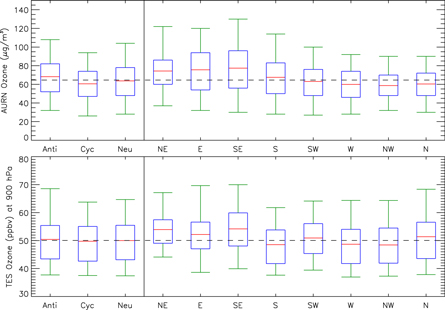
Figure 1. UK surface (top panel) and 900 hPa (bottom panel) summer-time (April–September) ozone from the Automated Urban Rural Network (AURN, 2006–2010 in μg m−3) and the tropospheric emission spectrometer (TES, 2005–2011 in ppbv), sampled under the synoptic classifications in the outer row and column of table 1. 'Anti', 'Cyc' and 'Neu' represent anticyclonic, cyclonic and neutral conditions, respectively. Other labels represent wind direction. Red is the cluster mean, blue is the cluster 25th and 75th percentiles and green is the 5th and 95th percentiles. Dashed lines show overall summer-time mean concentrations.
Download figure:
Standard image High-resolution imageIn all cases, the AURN and TES summer time ozone mean lies with the variability of different composite samples. Therefore, other processes such as tropospheric chemistry and emissions of precursor gases are important in governing UK ozone concentrations and so it is not possible, for example, to state that south-easterly summer conditions necessarily lead to ozone episode conditions. Different regions (e.g. South-East England; figure 2) will have stronger ozone responses than others to different weather regimes. So, the UK average pattern will be weaker than the most sensitive regions. Overall, the largest enhancements in UK average ozone concentrations in the vorticity and wind categories come from anticyclonic and south-easterly conditions, respectively. The significance of these regime responses is presented in figures 2 and 3. It should also be noted that there is also some overlap between anticyclonic and south-easterly conditions (i.e. in summer, 2005–2011, LWT 3 in table 1 made up 1.6% and 14% of the anticyclonic and south-easterly samples, respectively).

Figure 2. AURN summer-time surface ozone (μg m−3) sampled under (a) anticyclonic conditions and (b) south-easterly flow for 2006–2010. Panels (c) and (d) show the surface ozone anomalies relative to the seasonal average for the two synoptic conditions, respectively. Black polygonned regions show areas of significant difference between the composites and the seasonal average based on the Wilcoxon Rank Test (p < 0.05).
Download figure:
Standard image High-resolution image
Figure 3. TES summer-time vertical ozone profiles (ppbv) over the UK (12°W–6°E, 48°–62°N) between 2005 and 2011 sampled under anticyclonic (red), cyclonic (blue) and south-easterly (green) conditions. In panel (a) the black line is the summer-time average. The dotted lines show the variability (standard deviation) in the composite profiles. In panel (b) the profiles are shown relative to the seasonal average and the black dashed line is the zero bias line. Horizontal solid lines represent the profile uncertainty. Horizontal dashed/dotted lines show the tropopause height under the different synoptic conditions. The yellow region in both panels is the approximate region of peak TES sensitivity to retrieving lower tropospheric ozone. Squares and diamonds signify where the profiles are significantly different to the summer-time average at the 90% and 95% confidence levels.
Download figure:
Standard image High-resolution imageAs anticyclonic and south-easterly conditions coincide with the largest tropospheric ozone concentrations, the AURN and TES data during these regimes are investigated in more detail in figures 2 and 3. Under the anticyclonic conditions, UK surface ozone ranges from 50 to 80 μg m−3 (figure 2(a)). Larger UK surface ozone concentrations of between 60 and 100 μg m−3 are sampled under the south-easterly flow regime (figure 2(b)). Figures 2(c) and (d), show the surface ozone–synoptic composites with respect to the seasonal surface ozone average. The black polygonned regions show where the surface ozone anomalies are significantly different (p < 0.05) based on the Wilcoxon rank test (Pirovano et al 2012), as used by Pope et al (2014). Under both synoptic conditions, the surface ozone anomalies are significantly positive across the UK, indicating these synoptic conditions aid the accumulation and/or in situ production of ozone. The signal is more pronounced under south-easterly flow (>10 μg m−3) than anticyclonic conditions (0–5 μg m−3). Under anticyclonic conditions, atmospheric stability and light winds will trap ozone and its precursors, promoting in situ production. Less cloud cover will also tend to increase the ozone production rate. South-easterly flows transport surface ozone and precursors from continental Europe into the UK (Lee et al 2006), with ozone production occurring en route. Pope et al (2014) showed south-easterly flow transport of tropospheric column NO2 from the highly industrialised Benelux region, which would aid the formation of ozone downwind (i.e. over the UK).
As TES has limited spatial coverage, all summer-time ozone retrievals (vertical profiles) between 2005 and 2011 were averaged together over the UK (i.e. between 12°W–6°E and 48°–62°N). Figure 3(a) shows how all mean TES ozone profiles, sampled under the different weather conditions, increase with altitude from approximately 45–50 ppbv in the lower troposphere to 70–90 ppbv at 400 hPa, with increasing variability. Figure 3(b) presents the anomalies, relative to the seasonal average profile, for anticyclonic (LWT 0, red), cyclonic (LWT 20, blue) and south-easterly (LWTs 3, 13, 23, green) conditions. The horizontal bars represent the uncertainty/error range at the respective levels. The systematic errors cancel when differencing the vertical profiles and the random errors are reduced by 1/√N through averaging, where N is the number of vertical profiles (shown in the legend of figure 3(a)). Over-plotted squares and diamonds on the different profiles represent where the TES ozone synoptic weather composite and summer time means are significantly different at the 90% and 95% confidence levels. The yellow shading highlights the approximate region (900–650 hPa) of peak sensitivity of lower tropospheric ozone in the TES averaging kernels (AKs) (Worden et al 2013).
Under south-easterly conditions the TES ozone anomalies are qualitatively consistent with the AURN comparisons (figure 2), with significant (95% confidence) positive anomalies of 2.0–4.0 ppbv below 650 hPa. Under anticyclonic conditions between 900 and 825 hPa, there are small positive ozone anomalies of between 0.0 and 0.5 ppbv. Although the enhanced ozone signal can be detected outside of the measurement uncertainties/errors, the anomalies are non-significant. The signal below 900 hPa is significant (i.e. accumulation of ozone under anticyclonic conditions) but lies outside the AK sensitivity range. Above 800 hPa, the anomalies are significantly negative. When sampled under cyclonic conditions the opposite occurs with non-significant negative anomalies (–0.75–0.0 ppbv) between 900 and 825 hPa and significant positive biases (0–2.0 ppbv) between 800 and 650 hPa. This therefore suggests that there is a change in the response of tropospheric ozone through the profile under either weather regime.
Investigation of the process behind these TES ozone profiles is beyond the scope of this study and would require a detailed modelling and observational study. However, we can suggest some hypotheses. South easterly flows are indicative of continental air masses (i.e. continental Europe) which have spent a prolonged period over regions (e.g. the Benelux region) with anthropogenic emissions of ozone precursors. This would lead to increased ozone production compared to maritime air masses (e.g. south westerly flows) and hence a higher tropospheric column ozone which would over time be mixed throughout the troposphere. The average tropospheric column ozone mixing ratio is 75.1, 69.8 and 73.9 ppbv under south-easterly, anticyclonic and cyclonic conditions. This is supported by TES CO, sampled under south-easterly conditions (see SM), with its longer lifetime (i.e. several months), which also has significantly enhanced concentrations.
Under anticyclonic conditions vertical mixing is reduced and it is likely that this traps ozone and its precursors near the surface. The weaker vertical mixing also means fewer ozone precursors aloft leading to a reduced ozone production rate. Therefore, larger anticyclonic tropospheric columns (average tropopause height of 218.9 hPa, figure 3(b)) contain less ozone as it is trapped in the boundary level and clearer sky conditions aid its mid-upper tropospheric photochemical loss. Shallower cyclonic tropospheric columns (average tropopause height of 276.8 hPa), with enhanced vertical transport and reduced photochemical ozone loss from enhanced cloud cover, have higher tropospheric ozone concentrations. Other factors to be considered are the impact of the increased frequency of stratospheric intrusions under cyclonic conditions (O'Hare and Wilby 1995) and large-scale subsidence under anticyclonic flow.
3.2. Ozone-related health burden
Given its greater spatial resolution, we have used AQUM to evaluate the health burden linked to short-term surface ozone exposure under the different synoptic weather regimes. In the SM, we show that AQUM captures the midday surface ozone seasonal cycle seen in the AURN observations with a high correlation (0.83) and low mean bias (−6.03 μg m−3) within the observational uncertainty range (±9.68 μg m−3) for the whole year of 2006 (figure SM1). In addition, AQUM and AURN results were both sampled under anticyclonic and easterly/southerly (NE, E, SE and S) conditions for 2006 (see figure SM2) to see if AQUM can simulate the same AQ–synoptic weather relationships in summer-time seen in the observations. These synoptic regimes are chosen as they result in the largest ozone responses seen in figure 1. Overall, AQUM has similar positive anomalies, with respect to the seasonal average, to AURN for both synoptic groupings. The spatial anomaly correlations between AQUM and AURN are 0.55 and 0.62 for the anticyclonic and southerly/easterly conditions, respectively (95% confidence level). Therefore, we conclude that AQUM can generally reproduce the observational seasonal cycle and AQ-synoptic weather relationships.
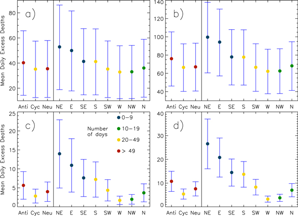
Using the scenarios listed in table 2, we investigate which of the summer-time synoptic conditions lead to the greatest MDEDR and how sensitive these results are to changes in the CRF and the use of a safe exposure limit. Each vorticity classification has 50 d or more of occurrence in this summer period. The wind regimes range from 0 to 49 d with peak occurrence in W, SW and S flows. The easterly (NE, E and SE) regimes have less occurrences, of between 0 and 9 d, over the summer period. In ExpA (using the non-seasonal CRF of β = 0.34% (0.12%, 0.56%) per 10 μg m−3 increase in ozone concentration and no threshold, table 2), among the vorticity regimes, anticyclonic conditions have the highest rate of approximately 41 excess deaths per day (d/day) in the UK (figure 4(a)). Among the wind regimes, easterly flows have the highest rates of 42–53 d/day. The same patterns occur for the other three scenarios (figures 4(b)–(d), even with the inclusion of a threshold, and in all experiments it is the NE flow that is associated with the greatest mortality rate. When we use a higher β = 0.65% (0.39%, 0.91%) in ExpB, this increases the RRs and AFs, which increases the MDEDR. Under anticyclonic conditions, there are approximately 76 d/day and the MDEDR under easterly flows ranges between 77 and 101 d/day (figure 4(b)). The remaining classifications range between 60 and 70 d/day. When the 70 μg m−3 threshold is used with β = 0.34% (0.12%, 0.56%) (ExpC; figure 4(c)), the rates for all conditions drop substantially to approximately 2–14 d/day. The easterly flows still have the largest MDEDR rate between 7 and 14 d/day. Anticyclonic conditions has rates of 5–6 d/day, while all other classifications have rates of less than 5 d/day. In ExpD, the 70 μg m−3 threshold reduces the rates to under 15 d/day for all classifications apart from the easterly flows which range between approximately 15 and 27 d/day (figure 4(d)). Anticyclonic conditions result in 10–11 d/day, which is the highest MDEDR of the vorticity regimes.
Figure 4. Mean daily excess mortality rate (d/day) from short-term exposure to surface ozone under different synoptic weather conditions during the summer (April–September) of 2006. The colour of the circle symbols indicates the number of days used to get the mean daily excess mortality rate from the different classifications. (a) ExpA: β = 0.34% (0.12%, 0.56%–95% confidence intervals) per 10 μ m−3 increase in surface ozone with no surface ozone threshold, (b) ExpB: β = 0.65% (0.39%, 0.91%) per 10 μ m−3 increase in surface ozone with no surface ozone threshold, (c) ExpC: β = 0.34% (0.12%, 0.56%) per 10 μ m−3 increase in surface ozone with a threshold of 70 μg m−3, (d) ExpD: β = 0.65% (0.39%, 0.91%) per 10 μ m−3 increase in surface ozone with a threshold of 70 μg m−3.
Download figure:
Standard image High-resolution image
Overall, anticyclonic and easterly (especially NE) conditions produce the highest MDEDRs under all the scenarios in table 2. Favourable meteorology conditions and transport of pollution from continental Europe aid the accumulation and formation of ozone, enhancing the UK concentrations and the associated health effects. Changes in CRFs between ExpA and ExpB increase MDEDRs by nearly a factor of 2. When no safe exposure limit is used, the death rates are larger but the relative difference between synoptic classifications is smaller. The inclusion of the safe exposure limit reduces the MDEDRs beteen ExpA/ExpB and ExpC/ExpD by a factor of 4–5, but now the death rates are more dependent on the weather classification (i.e. less overlap between the synopitc weather uncertainty ranges).
We suggest that ExpA is the best estimate of MDEDR as there is no clear evidence for a concentration threshold (Bell et al 2006, COMEAP 2015) and the CRF is based on multiple studies (COMEAP 2015). Therefore, the estimated MDEDR under anticyclonic conditions is approximately 41β = 0.34% (14β = 0.12%, 66β = 0.56%) d/day and under easterly conditions of 42–53β = 0.34% (15–19β = 0.12%, 67–87β = 0.56%) d/day in the summer of 2006.
4. Conclusions
We have investigated the links between synoptic weather and air quality in the UK focussing on summer-time (April—September) observations of surface/tropospheric ozone and objective LWTs (daily midday classification of UK atmospheric circulation). Observations from both AURN and TES show significantly enhanced surface and 900–800 hPa ozone concentrations under anticyclonic and easterly (NE, E and SE) conditions, relative to the summer-time average. Cyclonic and westerly (SW, W and NW) conditions were found to reduce surface/900–800 hPa ozone, relative to the summer-time average, as cleaner Atlantic air is transported over the UK.
The Met Office AQUM successfully reproduced the synoptic weather–surface ozone relationships seen in the observations, and hence due to its greater spatial resolution was used to assess the health burden of short-term exposure to enhanced surface ozone. The MDEDR due to enhanced surface ozone concentrations was calculated for the different synoptic regimes with peak MDEDRs under summer-time anticyclonic and easterly conditions. The MDEDR is sensitive to changes in the CRF (β = 0.34% and 0.65% per 10 μg m−3 increase in surface ozone) and including a safe exposure limit of 70 μg m−3. Since there is no clear evidence for a concentration threshold and the CRF (i.e. β = 0.34% per 10 μg m−3 increase in surface ozone) is based on multiple studies, we provide a best estimate for MDEDR under anticyclonic conditions of approximately 41 (14, 66) d/day and under easterly conditions of 42–53 (15–19, 67–87) d/day in the summer of 2006.
Overall, this study has shown that the LWTs are a powerful tool to better understand the influence of synoptic weather on UK summer-time surface/tropospheric ozone concentrations. When the UK experiences strong anticyclonic events or easterly winds during summer, surface ozone conditions are likely to be enhanced and the risk of adverse health impacts increases. Therefore, it is important for air quality models to able to accurately reproduce these synoptic weather–surface ozone relationships in their forecasts and that authorities prepare for, and are able to mitigate, the associated heath impacts.
Acknowledgments
This work was supported by the UK Natural Environment Research Council (NERC) through funding for the National Centre for Earth Observation (NCEO). We acknowledge the use of the TES ozone data, provided by NASA JPL, which is available at http://reverb.echo.nasa.gov/reverb/. We also acknowledge the use of the AURN ozone data, provided by the Department for Environment, Food and Rural Affairs, which is available at https://uk-air.defra.gov.uk/networks/network-info?view=aurn. We thank the Climate Research Unit, University of East Anglia, for the Lamb Weather Type data (https://crudata.uea.ac.uk/cru/data/lwt/).