


ABSTRACT
Two techniques, the Partial Variance of Increments (PVI) and the Local Intermittency Measure (LIM), have been applied and compared using MESSENGER magnetic field data in the solar wind at a heliocentric distance of about 0.3 AU. The spatial properties of the turbulent field at different scales, spanning the whole inertial range of magnetic turbulence down toward the proton scales have been studied. LIM and PVI methodologies allow us to identify portions of an entire time series where magnetic energy is mostly accumulated, and regions of intermittent bursts in the magnetic field vector increments, respectively. A statistical analysis has revealed that at small time scales and for high level of the threshold, the bursts present in the PVI and the LIM series correspond to regions of high shear stress and high magnetic field compressibility.
Export citation and abstract BibTeX RIS
1. INTRODUCTION
In-situ spacecraft observations have revealed that the solar wind is a turbulent magnetized plasma characterized by a very broad electromagnetic power spectrum that encompasses time scales from several hours to about 0.01 s. Under the assumption of the Taylor frozen-in hypothesis (Taylor 1938), this corresponds to a wide range of spatial scales, as well. At time scales larger than the ion-gyroscale (i.e., in the inertial range) the power spectral density follows a power law decay f−5/3 (Matthaeus & Goldstein 1982; Tu & Marsch 1995), in analogy with the velocity power spectrum in non-magnetized fluids. At smaller time scales, where the ion physics becomes dominant, a second, steeper spectral range has been found (Leamon et al. 1998; Bale et al. 2005). Recent analysis have pointed out that this second spectral range extends down to electron scales (Sahraoui et al. 2009, 2010). Another study on 100 spectra measured by the STAFF instrument on board Cluster has revealed that the power spectral density from ions to electron scales is better fitted by an exponential function (Alexandrova et al. 2009, 2012). Although the spectral properties of magnetic field fluctuations in the solar wind from ion to electron scales are still matter of debate, the magnetic field, both in the inertial and in the high frequency range, have been found to be spatially characterized by discontinuities (Burlaga 1969; Tsurutani & Smith 1979; Li 2008; Perri et al. 2012b). Solar wind discontinuities are usually identified as abrupt changes in the plasma and in the magnetic field (Tsurutani & Smith 1979). Historically, the classification of interplanetary discontinuities into categories such as directional discontinuities (DDs), rotational discontinuities (RDs), and tangential discontinuities (TDs) has been based on linear ideal MHD theory (Neugebauer 2006). There are also differences in their interpretation: one familiar view is that discontinuities are static boundaries between flux tubes originating in the lower corona (or photosphere). In this "spaghetti" view, the tubes may tangle up in space, but remain distinct entities (Mariani et al. 1973; Bruno et al. 2001). Another interpretation is that some of the observed discontinuities might be the current sheets that form as a consequence of the cascade of MHD turbulence to inertial scales and down (Greco et al. 2009). However, distinguishing between the two scenarios is not trivial and the results coming from data analysis at various scales have always been treated with caution.
On the other hand studies on hydrodynamics and MHD pointed out that fully developed turbulence presents an energy cascade characterized by intermittency, namely, the distribution of the field differences strongly deviates from a Gaussian as the spatial scale decreases (Biskamp 1993; Frisch 1995; Sreenivasan & Antonia 1997). This effects is due to the appearance of coherent structures that give rise to an increasing spatial non-homogeneity. These structures play a crucial role in turbulence since they might be sites of enhanced non uniform dissipation. The conjectured relationship between the statistics of dissipation and the statistics of small scale fluctuations is known as Refined Similarity Hypothesis (Kolmogorov 1962; Sreenivasan & Antonia 1997), which although unproven, provides theoretical underpinning to the studies of multifractals and other scaling behavior. Intermittency has also been observed extensively in the solar wind (Marsch & Tu 1994; Horbury & Balogh 1997; Sorriso et al. 1999).
In recent years, the study of the formation of coherent structures in space plasmas has gained considerable attention in identification methods (Bruno et al. 2001; Hada et al. 2003; Greco et al. 2008), in observational evidences (Salem et al. 2009; Greco et al. 2012a; Perri et al. 2012b; Zhdankin et al. 2012), and in relevant simulation results (Wan 2012; Wu et al. 2013). Solar wind observations and numerical simulations showed that current sheets are associated with enhanced heating (Osman et al. 2011), distortions of proton distribution functions have been found to be concentrated near coherent structures (Greco et al. 2012b), some of the plasma instabilities in the solar wind seem to develop close to magnetic discontinuities (Malaspina et al. 2013), and a temporal association of energetic particle fluxes with these coherent structures exists, suggesting that certain mechanisms for suprathermal particles acceleration operate preferentially close to (but not in) magnetic discontinuities (Tessein et al. 2013). Thus, studying properties of discontinuities in the interplanetary space over a broad range of time scales has a consistent impact in addressing processes at fluid, proton, and electron scales.
This work compares two methodologies for detecting magnetic discontinuities in the solar wind flow, making use of the MESSENGER magnetic field data in the inner heliosphere at a resolution of 2 vec s−1.
We will describe the two methodologies in Section 2. Then, the main results will be presented and commented in Section 3; while in Section 4, we will discuss the implications of our statistical study in the investigation of the dynamics of solar wind discontinuities.
2. METHODOLOGIES
The purpose of the present analysis is to compare the results coming from two methods that allow us to pick up "energetic events" in the magnetic field fluctuations.
The Partial Variance of Increments (PVI) technique (Greco et al. 2008) is sensitive to rapid changes in the magnetic field components,

where  is the magnetic field vector and Δt is a time separation. The expression in Equation (1) indicates the increments of the magnetic field vector. Thus, the PVI can be defined via the normalized quantity
where 〈•〉 denotes a temporal average over the entire data set. The capability of the PVI approach to identify discontinuities has been shown to be comparable to standard methods in both MHD simulations and solar wind observations, and it has become clear that the properties of coherent structures can be meaningfully related to what have been called classical or ideal discontinuities (Greco et al. 2008, 2009). Note that by construction 〈PVI〉 = 1, while 〈PVI2〉 is related to the kurtosis of the increments of the magnetic field components. Furthermore, higher order moments of 〈PVI〉 exhibit a scaling that is related to classical diagnostics of intermittency (as, for example, the structure functions (Bruno & Carbone 2005)).
On the other hand, the Local Intermittency Measure (LIM; Farge et al. 1990) technique is based on the wavelet analysis of the magnetic field components allowing the identification of large amplitude bursts of magnetic energy at different time scales and at particular times. Indeed,
where  is the sum over the square of the wavelet coefficients of the magnetic field components at time t and time scale Δt. In other words, Equation (3) indicates that for each time scale Δt, a value of LIM > 1 identifies portions of the sample whose power (the squared wavelet coefficient) is above the average, namely, a region where magnetic energy has accumulated. Note that Equation (3) has the same physical meaning as the second order structure function and should have the same scaling laws. By construction 〈LIM〉 = 1 and 〈LIM2〉 is related to the kurtosis of the signal. The wavelet coefficients
  are computed by choosing an arbitrary wavelet function ψ. For this analysis, we used a discrete Haar mother wavelet
ψ(t) functions form an orthonormal space of square-integrable functions on the unitary interval [0, 1]. Owing to its particular shape, Haar function is well suited for studying discontinuities (Veltri & Mangeney 1999; Bruno et al. 2001).
Thus, both the techniques are able, for some imposed conditions (i.e., thresholds), to select parts of a data sample where large amplitude variations in the magnetic field vector and in the magnetic energy are present. In this analysis, we indeed fixed thresholds with amplitudes from 〈•〉 + σ to 〈•〉 + 5σ both in the PVI and in the LIM time series simultaneously, where 〈•〉 and σ are the average and the rms of the LIM and PVI signals, respectively (〈•〉 = 1 and σ varies between 3.5 and 2.5 from Δt = 2 s to Δt = 16 s). With this choice, we do not impose the same numerical value of the threshold on both signals, but rather we select parts of the two series that have the same σ above their average.
Furthermore, both the PVI and the LIM have been computed at four different time scales, namely, Δt = 2, 4, 8 and 16 s.
3. DATA ANALYSIS AND RESULTS
The data analysis is performed on an Alfvénic stream as detected by the MESSENGER spacecraft in the inner heliosphere at ∼0.3 AU. That stream has been presented in Perri et al. (2012a) and is characterized by large amplitude magnetic field fluctuations into the plane perpendicular to the solar wind radial direction; notice that at 0.3 AU, the radial direction is almost parallel to the Parker spiral; therefore, evidence suggests the presence of Alfvénic fluctuations. The data have been acquired by the magnetometer on board MESSENGER at the rate of 2 vec s−1 (Anderson et al. 2007). The magnetic field time series has been observed during the day 2010 January 14 (about 236191 points), within the solar minimum of the solar cycle 23 in order to minimize the presence of large-scale transient structures. It is worth remembering that those data allow us to perform a time-scale-dependent analysis from the inertial range scales down to about the proton scales; indeed, since the mean field magnitude of the stream is 〈|B|〉 ∼ 25 nT, the proton cyclotron frequency is fcp ∼ 0.38 Hz, while the Nyquist frequency of the data is 1 Hz. Notice that it is not possible to give an estimation of the Doppler-shifted frequencies corresponding to the proton gyroradius and to the proton inertial length owing to the unavailability of the plasma data on MESSENGER spacecraft.
Examples of the time behavior of the PVI and of the LIM measures are shown in Figure 1 at two different time scales, i.e., Δt = 2 s (top panels) and Δt = 16 s (bottom panels). Notice the burstiness of the signals at both the scales, that suggests the presence of sharp gradients and localized enhancements of magnetic energy in the time series. The application of a threshold on either the PVI and the LIM series permits to select events, such as magnetic discontinuities and regions of high magnetic stress, leading to a hierarchy of coherent structures. Indeed, higher and higher values of that threshold can pick up portions of the signal where rapid and abrupt enhancements in the magnetic energy are present. From the solar wind magnetic field data analysis, those large amplitude variations have been routinely ascribed to "rare" events that change the probability distribution function of the field increments from being Gaussian to develop highly non-Gaussian tails (Greco et al. 2012a). Those tails become fatter and fatter with high kurtosis as the time scale decreases (intermittency) (Marsch & Tu 1994; Sorriso et al. 1999; Bruno et al. 2001), suggesting an increase in the spatial non-homogeneity of the field going toward smaller scales. However, a very recent study performed on the same MESSENGER data set (Perri et al. 2012a) has shown that the occurrence of bursts of magnetic energy of any amplitude plays a fundamental role in the nonlinear transfer of magnetic energy through the inertial range and beyond. However, in this work, we want to characterize the spatial properties of the magnetic field fluctuations only for extreme events, as selected via an arbitrary threshold and captured by two different methods of analysis, although also the remaining signal, which composes the whole distribution function of the magnetic field increments, is fundamental for the development of the magnetic energy cascade.
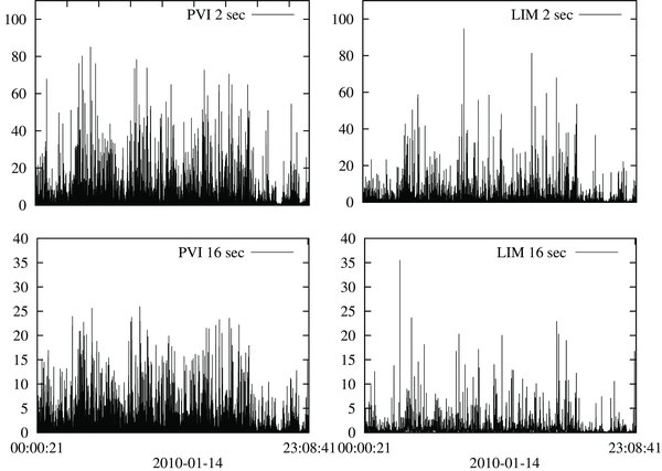
Figure 1. PVI (left columns) and LIM (right columns) series at Δt = 2 s (top panels) and Δt = 16 s (bottom panels).
Download figure:
Standard image High-resolution imageAt this point, we can define one set of elements consisting of structures detected by the LIM technique and another one of structures identified by the PVI method. Thus, it is possible to adopt a procedure that counts how many events are identified as both LIM and PVI events. Each discontinuity in the signal is bounded between a starting and an ending time. When the time interval of the identified PVI discontinuity above the threshold overlaps (partially or totally) with the time interval of the identified LIM discontinuity (above the same threshold), the structure is recorded as PVI/LIM event. Otherwise the PVI event is not identified with any peak in the LIM series. The results of this procedure are reported in Tables 1, 2, and 3, which summarize the number of LIM, PVI, and PVI/LIM structures detected for three different values of the arbitrary threshold and at different time scales Δt.
Table 1. Number of LIM, PVI, and PVI/LIM Structures as a Function of Δt for a Threshold =1 + σ
| LIM | PVI | PVI/LIM | |
|---|---|---|---|
| 2 s | 1095 | 4756 | 1656 |
| 4 s | 628 | 4059 | 1220 |
| 8 s | 357 | 3489 | 921 |
| 16 s | 195 | 3206 | 715 |
Download table as: ASCIITypeset image
Table 2. Number of LIM, PVI, and PVI/LIM Structures as a Function of Δt for a Threshold =1 + 3σ
| LIM | PVI | PVI/LIM | |
|---|---|---|---|
| 2 s | 333 | 1430 | 411 |
| 4 s | 205 | 1196 | 287 |
| 8 s | 110 | 1020 | 216 |
| 16 s | 57 | 856 | 144 |
Download table as: ASCIITypeset image
Table 3. Number of LIM, PVI, and PVI/LIM Structures as a Function of Δt for a Threshold =1 + 5σ
| LIM | PVI | PVI/LIM | |
|---|---|---|---|
| 2 s | 168 | 704 | 189 |
| 4 s | 85 | 583 | 111 |
| 8 s | 47 | 434 | 73 |
| 16 s | 22 | 371 | 43 |
Download table as: ASCIITypeset image
The number of bursty variations increases on smaller scales, being a clear evidence of intermittency. Note that the number of PVI/LIM structures is larger than the number of LIM events. This is due to the fact that in the same time interval during which a LIM event is above a given threshold, two or more PVI events could be simultaneously above that threshold. This strongly depends on the time width of the mother wavelet ψ(t) chosen for computing the LIM (a better temporal resolution in the wavelet function corresponds to a greater uncertainty in the scale resolution and vice versa, so that results from the LIM analysis are obviously influenced by this choice). The Haar wavelet has given the better accordance with the PVI method. It is further clear that all the LIM structures are PVI events, but it has also been observed a complementary set of discontinuities detected by the PVI method but not by LIM (as can be easily deduced by Tables 1, 2, and 3).
To characterize the magnetic energy enhancements, we have computed the rotation angle θ for each structure in Tables 1, 2, and 3, as the maximum value of
(Vasquez et al. 2007; Borovsky 2008; Perri et al. 2012b; Zhdankin et al. 2012), where t0 = 0.5 s, and δB(t) ≡ B(t) − B0 are the magnetic field fluctuations (B0 being the large-scale magnetic field that has been computed at the integral time scale T0 = ∫Eb(f)f−1 df/∫Eb(f)df ∼ 1 hr, where Eb(f) is the isotropic magnetic power spectrum and f is the frequency; Sorriso-Valvo et al. 2006).
In addition, we have calculated the magnetic compressibility within each structure,
as defined in Bruno et al. (2007). In Equation (6), the numerator represents the standard deviation of the magnetic field intensity computed over a certain time window which corresponds to the duration of the discontinuity, and the denominator is the square value of the total magnetic field magnitude averaged over the whole duration of the data set. SB gives an indication of the degree of compressibility of the magnetic field fluctuations; previous studies on Helios data in the inertial range have highlighted SB < 10−3 (Bavassano et al. 1982), namely, a very low compressibility.
Some examples of PVI/LIM structures on Δt = 2 s are reported in Figure 2. In each plot, the three components of the magnetic field in the minimum variance reference frame are displayed, along with the magnitude of the magnetic field vector (see figure legend).
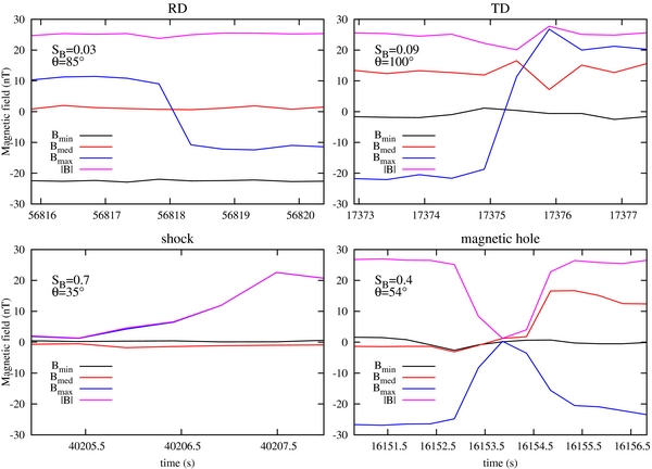
Figure 2. Examples of PVI/LIM structures. The plots show the three components of the magnetic field in the minimum variance reference frame and the magnitude of the magnetic field vector. The maximum values of the rotation angle θ and the magnetic compressibility SB are also reported in the panels.
Download figure:
Standard image High-resolution imageThe structure on the top left is almost incompressible (the module of B is constant), having a well defined direction of maximum variance. The minimum variance analysis applied to this event shows that the maximum variance direction (Bmax) changes sign and rotates by an angle of about 85°. The normal component Bmin is different from zero, so this structure might be classified, according to the ideal MHD, as an RD. It has been shown by Hudson (1970) that under the assumption of isotropic plasma, RDs are characterized by a continuous |B| across the discontinuity and by continuous density and pressure, thus a small value of SB implies a pressure balanced incompressible structure. In the case of continuous density and magnetic field magnitude, a continuous pressure is also found for anisotropic plasmas (Hudson 1970). On the top right, we show a TD: Bmax performs a large rotation and Bmin is almost zero and the magnetic field magnitude undergoes a change of roughly 10 nT.
The structures on the bottom are two compressive discontinuities. We tentatively define the event on the left as a shock, due to the abrupt increase seen in the magnetic field intensity (however, it is not possible to check that owing to the unavailability of plasma data on MESSENGER spacecraft), and the event on the right as a magnetic hole (Turner et al. 1977; Winterhalter et al. 1994; Zhang et al. 2008; Salem et al. 2009), because of the deep depression in the magnitude of B. These four examples reveal the large variety of magnetic structures that can be detected by the two methods.
Since the events picked up by the two methods exhibit various properties, we tried to infer particular features (if any) via a statistical analysis throughout the entire data set and for different values of the time scales and of the thresholds. Figure 3 shows the scatter plots of the magnetic field compressibility SB as a function of the angle of rotation of B for a threshold value 1 + 3σ and for Δt = 2 s (left columns) and Δt = 8 s (right columns). The top panels display only PVI events, while the bottom panels show those LIM events that are also detected by the PVI procedure (red open circles), in order to highlight differences and analogies. It is evident that a correlation between the magnetic compressibility and the rotation angle exists, indeed high shear structures (>60°) tend to be highly compressible (>0.1), in agreement with other statistical studies, in which magnetic discontinuities with more reversed field vector have enhanced field depression as well (Vasquez et al. 2007; Zhang et al. 2008; Malaspina et al. 2013). The correlation coefficients is ∼0.66–0.75 for both PVI and PVI/LIM events at the two time scales shown in Figure 3. In order to show the linear trend associated with this correlation, we over-plot the averages of SB in bins of θ. Although the correlation values are pretty high and a good linear trend is visible, a noticeable spread of the events is present.
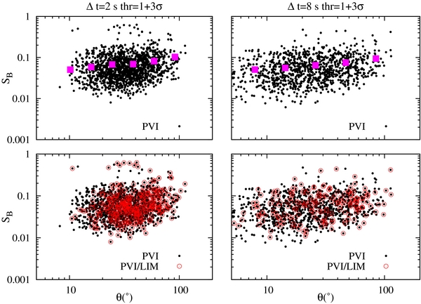
Figure 3. Scatter plots of the magnetic compressibility SB vs. the rotation angle θ for each structure detected by the PVI method (first row) in logarithmic scale. We overplot the averages of SB calculated in bins of θ (magenta full squares) to highlight the linear trend. In order to facilitate the comparison, the structures of the first row are depicted together with those detected simultaneously by the PVI and LIM methods (second row). The left columns refer to Δt = 2 s and the right ones to Δt = 8 s, both for threshold =1 + 3σ.
Download figure:
Standard image High-resolution imageIt is interesting that low shear structures (<10°) are present only on larger scales and especially, in PVI data set, and they completely disappear at Δt = 2 s. A similar conclusion can be inferred from scatter plots displayed in Figure 4 for Δt = 2 s and for three different values of the threshold. It is clear that the higher the threshold is the less populated is the region with low θ; however, the threshold level does not affect the distribution of the events with respect to the SB values. In other words, very bursty structures in both the PVI and the LIM series tend to correspond to magnetic discontinuity with a field vector that performs large amplitude rotations and with a level of magnetic compressibility that can be both high or low.
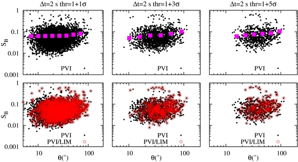
Figure 4. Same as Figure 3 but for a time scale Δt = 2 s and three different values of the threshold (from left to right).
Download figure:
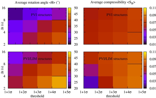
Standard image High-resolution imageIn order to highlight the dependence of θ and SB on the threshold values and on the time scales, we have constructed bi-dimensional histograms of the average values of the above quantities for both PVI and PVI/LIM events (see Figure 5). The trend of the average value of the rotation angle indicates again an increase of its values as Δt decreases and the threshold amplitude increases, so that we deduce that large amplitude abrupt rotations become more frequent going toward the proton scales. For the rotation angle of PVI/LIM discontinuities, the average values are slightly larger. The histograms in Figure 5, displaying the average value of the magnetic compressibility as a function of the threshold and of the time scale, confirm, as deducted by the scatter plots in Figure 4, that the dependence of SB on these two quantities is weaker than θ, although the very large values for the compressibility are more probable at high threshold values (this is more evident for PVI/LIM events). Thus, the latter suggests that the portions of both PVI and LIM signals, indicating a greater accumulation of magnetic energy, can be associated with statistical significance to high stressed discontinuities and only few of them are also characterized by a high level of compressibility. Those structures seem to be more predominant toward smaller time scales and could probably be thin current sheets, as those observed around the proton scales in the pristine solar wind at 1 AU by Perri et al. (2012b).
Figure 5. First column: two dimensional maps of the average values of the rotation angle 〈θ〉 detected by the PVI method and by the PVI and LIM methods simultaneously as a function of the time scale Δt and the threshold. Second column: two dimensional maps of the average values of the magnetic compressibility 〈SB〉 detected by the PVI method and by the PVI and LIM methods simultaneously as a function of the time scale Δt and the threshold.
Download figure:
Standard image High-resolution image
4. DISCUSSION
This paper presented a comparison between two methodologies for detecting magnetic discontinuities in the solar wind. That comparison has been made using a threshold method for selecting events in the time series that exhibit a very high level of magnetic energy. Each structure has been characterized by an angle of rotation of the magnetic field vector and by the compressibility of the fluctuations. The two methods lead to almost the same results, however, there has been found a subclass of discontinuities detected mostly by PVI but not by LIM: those are low shear structures (i.e., θ < 10°), which in turn, could be also associated with reconnection sites, as shown recently by Gosling & Phan (2013), and therefore be fundamental for energy dissipation in the solar wind plasma.
The statistical analysis as a function of the time scales has revealed an increase of high shear discontinuities toward smaller scales, while no clear dependence on Δt has been detected for the compressibility of the magnetic field fluctuations. A similar result comes from the threshold study, namely, high thresholds select mostly large amplitude rotations in the field vector but the range of variability for SB remains almost unchanged (see Figure 4). Thus, magnetic discontinuities are characterized by a broad range of physical properties at small scales (see Figure 2), although high shears seem to become dominant.
Further, since the majority of discontinuities exhibit 0.01 < SB < 0.1, that is a pretty low level of compressibility (see Figures 3 and 4), it seems that there is a consistency with the results shown in Vasquez et al. (2007); Zhang et al. (2008), and more recently in Wang et al. (2013), where an analysis on magnetic field data at different heliocentric distances revealed an abundance of incompressible discontinuities and a rare detection of compressive ones, where higher SB values are expected. Therefore, the very low level of magnetic compressibility found by Bavassano et al. (1982) in the Helios data persists also toward those scales where the ion physics becomes dominant.
It would be worth studying the correlation between θ and SB at smaller scales where the electron physics becomes dominant and establishing whether those properties evolve as a function of the heliocentric distance. Further investigation of magnetic discontinuities at electron scales in the inner heliosphere, as well as on the possibility of being sites of magnetic reconnection and energy dissipation, will be probably feasible with the forthcoming missions Solar Orbiter and Solar Probe Plus.
The authors would like to acknowledge helpful conversations with P. Veltri, B. Matthaeus and M. Goldstein. S.P.'s research was supported by "Borsa Post-doc POR Calabria FSE 2007/2013 Asse IV Capitale Umano, Obiettivo Operativo M.2." A.G. and S.P. further acknowledge the Marie Curie Project FP7 PIRSES-2010-269297 "Turboplasmas."