Use and misuse of temperature normalisation in meta-analyses of thermal responses of biological traits

Dimitrios - Georgios Kontopoulos; Bernardo García-Carreras; Sofía Sal; Thomas P. Smith; Samraat Pawar

doi:10.7717/peerj.4363

Use and misuse of temperature normalisation in meta-analyses of thermal responses of biological traits

Dimitrios - Georgios Kontopoulos ^1,2, Bernardo García-Carreras², Sofía Sal², Thomas P. Smith², Samraat Pawar²

1Science and Solutions for a Changing Planet DTP, Imperial College London, London, United Kingdom

2Department of Life Sciences, Silwood Park, Imperial College London, Ascot, Berkshire, United Kingdom

DOI: 10.7717/peerj.4363

Published: 2018-02-09
Accepted: 2018-01-23
Received: 2017-07-10

Academic Editor: Benjamin Letcher

Subject Areas: Ecology, Mathematical Biology, Climate Change Biology
Keywords: Sharpe-Schoolfield, Thermal response, Physiology, Temperature

Copyright: © 2018 Kontopoulos et al.
Licence: This is an open access article distributed under the terms of the Creative Commons Attribution License, which permits unrestricted use, distribution, reproduction and adaptation in any medium and for any purpose provided that it is properly attributed. For attribution, the original author(s), title, publication source (PeerJ) and either DOI or URL of the article must be cited.

Cite this article: Kontopoulos D-G, García-Carreras B, Sal S, Smith TP, Pawar S. 2018. Use and misuse of temperature normalisation in meta-analyses of thermal responses of biological traits. PeerJ 6:e4363 https://doi.org/10.7717/peerj.4363

The authors have chosen to make the review history of this article public.

Abstract

There is currently unprecedented interest in quantifying variation in thermal physiology among organisms, especially in order to understand and predict the biological impacts of climate change. A key parameter in this quantification of thermal physiology is the performance or value of a rate, across individuals or species, at a common temperature (temperature normalisation). An increasingly popular model for fitting thermal performance curves to data—the Sharpe-Schoolfield equation—can yield strongly inflated estimates of temperature-normalised rate values. These deviations occur whenever a key thermodynamic assumption of the model is violated, i.e., when the enzyme governing the performance of the rate is not fully functional at the chosen reference temperature. Using data on 1,758 thermal performance curves across a wide range of species, we identify the conditions that exacerbate this inflation. We then demonstrate that these biases can compromise tests to detect metabolic cold adaptation, which requires comparison of fitness or rate performance of different species or genotypes at some fixed low temperature. Finally, we suggest alternative methods for obtaining unbiased estimates of temperature-normalised rate values for meta-analyses of thermal performance across species in climate change impact studies.

Introduction

Temperature is a key factor that directly or indirectly governs the performance of biochemical reaction rates, physiological rates (e.g., respiration and photosynthesis), and even ecological rates (e.g., prey encounter rate). Understanding how biological rates respond to changes in environmental temperature (the thermal performance curve, TPC; Fig. 1) is important for ecological and comparative evolutionary analyses of thermal physiology, for better predicting how climate change will influence the dynamics of populations, communities, and ecosystems (Brown et al., 2004; Pörtner et al., 2006; Dell, Pawar & Savage, 2011; Hoffmann & Sgrò, 2011; Schulte, Healy & Fangue, 2011; Pawar, Dell & Savage, 2015). Another example of such analyses involves testing the hypothesis of metabolic cold adaptation (MCA; e.g., see Seibel, Dymowska & Rosenthal, 2007; White, Alton & Frappell, 2012; Clarke, 2017), according to which cold-adapted individuals exhibit higher metabolic rates at low temperatures (well below T_pk; see Fig. 1) than individuals adapted to higher temperatures.

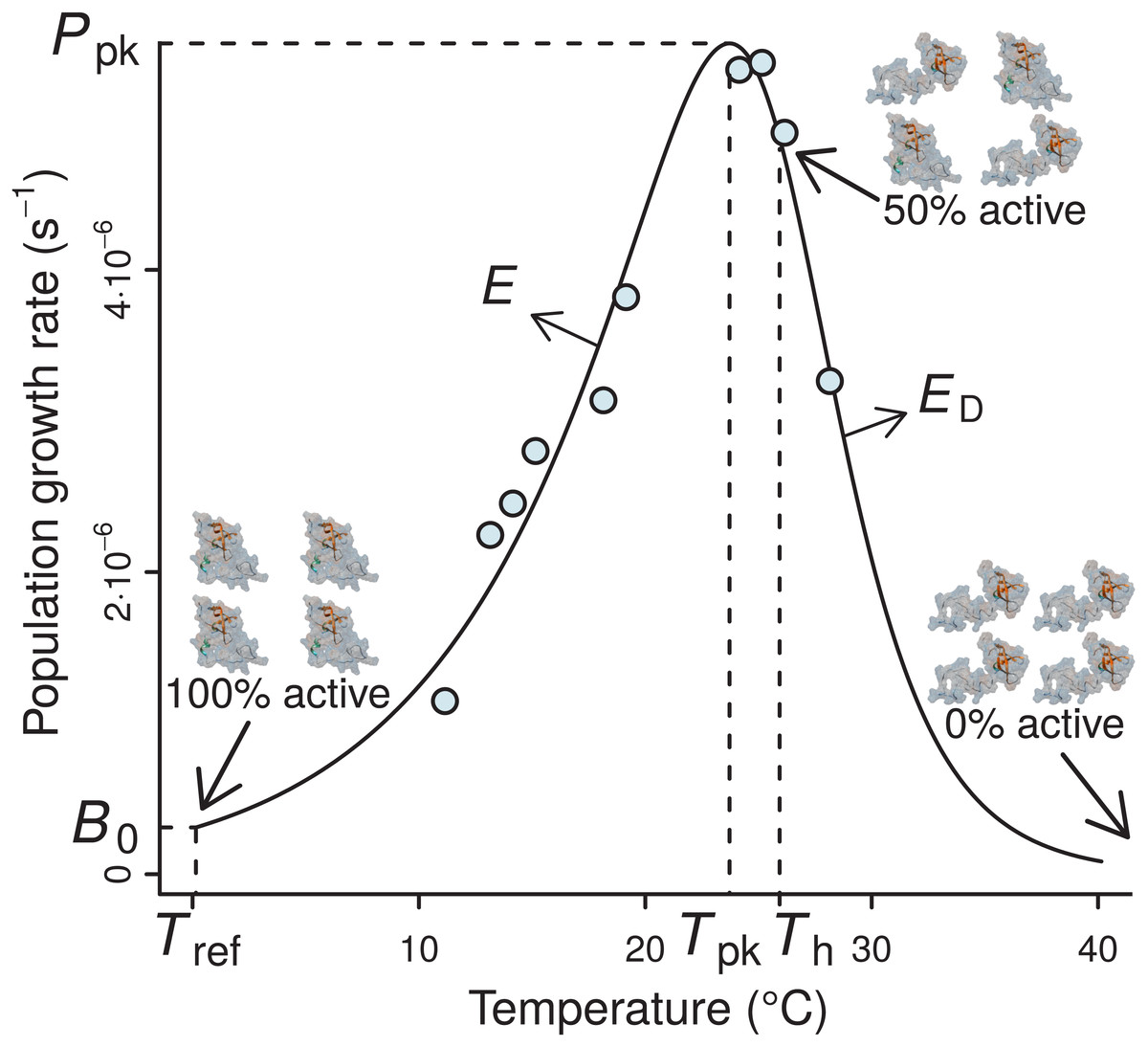
A typical example of the four-parameter Sharpe-Schoolfield model fitted to a thermal performance curve of Prochlorococcus marinus strain MIT9515 (Johnson et al., 2006). — Figure 1: A typical example of the four-parameter Sharpe-Schoolfield model fitted to a thermal performance curve of *Prochlorococcus marinus* strain MIT9515 (Johnson et al., 2006).
As depicted, the model assumes that the activity of a single rate-controlling enzyme controls the apparent temperature dependence of the rate. T_h is defined as the temperature (before or after the peak) at which 50% of enzyme units are made inactive. Beyond T_h, an increasing proportion of the enzyme population is deactivated, to the point where all of them become non-functional, and the curve falls to zero. B₀ accurately represents the real rate performance at a reference temperature (T_ref), only if the enzyme population is fully functional at this particular T_ref, i.e., T_ref ≪ T_h; otherwise, B₀ will necessarily be greater than the real rate value at T_ref (B(T_ref)).

Download full-size image

DOI: 10.7717/peerj.4363/fig-1

The TPCs of fundamental biological rates (traits) are generally unimodal, and biological rate versus temperature relationships are typically well-described by mathematical models that quantify four key features of the response: the temperature where the performance peaks (T_pk), the rate performance at a reference temperature (B₀), typically well below T_pk within its operational temperature range (Pawar et al., 2016), the rise of the rate up to T_pk (E), and the fall after T_pk (E_D) (Fig. 1). The normalised rate value B₀ is particularly important, as it allows rate performance to be standardised for comparison across individuals and species (Gillooly et al., 2001). In particular, the inference of normalised rate values at a reference temperature between species is key for studying MCA, or for comparisons of the performance of different biological rates (e.g., photosynthesis and respiration) at a common temperature (e.g., see Padfield et al., 2017).

Partly mechanistic models that explicitly link a cellular, organismal, or population rate’s value to the temperature-dependence of the underlying biochemical kinetics (e.g., Johnson & Lewin, 1946; Sharpe & DeMichele, 1977; Schoolfield, Sharpe & Magnuson, 1981; Ikemoto, 2005; Corkrey et al., 2012; Hobbs et al., 2013; DeLong et al., 2017) are becoming increasingly popular for quantifying empirically observed TPCs (Hochachka & Somero, 2002). Such models have occasionally received criticism on the grounds that they only constitute phenomenological statistical descriptions, as their assumptions are too simplistic and cannot be directly mapped onto physiological or ecological rates, which should be driven by a far more complex interplay of processes (e.g., Clarke, 2004; Clarke & Fraser, 2004; Clarke, 2006; Clarke, 2017; but see Gillooly et al., 2006). Nevertheless, these models continue to be used in the literature as they can adequately fit a large variety of experimentally determined TPCs, enabling the quantification of various aspects of the shape of the performance curve.

Among these models, the Sharpe-Schoolfield model (Schoolfield, Sharpe & Magnuson, 1981) has been frequently used in recent studies to address both ecological and evolutionary questions about the effects of temperature change on individuals, populations, and communities (Barmak et al., 2014; Barneche et al., 2014; Fand et al., 2014; Simoy, Simoy & Canziani, 2015; Barneche et al., 2016; Padfield et al., 2016; Vimercati et al., 2016). In particular, the B₀ calculated from fitting this model to TPC data has been used to compare the rate performance of different species (e.g., Wohlfahrt et al., 1999), treatments (e.g., Padfield et al., 2016), or developmental stages (e.g., Hopp & Foley, 2001) at a reference temperature, T_ref. However, the implicit assumption made by these studies, that B₀ is exactly the normalised rate value at T_ref, is only valid under certain conditions (see the Theoretical context section), and may in fact heavily overestimate the actual rate value at that temperature (Schoolfield, Sharpe & Magnuson, 1981) (Fig. 1). Such an overestimation could introduce unexpected biases not only in comparisons of temperature-normalised rates (among e.g., species, treatments, or developmental stages), but also in other analyses (e.g., exaggerating the rate performance of cold-adapted species could provide false support for MCA in its absence).

Here, we study the likely incidence of this overestimation of the normalised B₀ obtained by fitting the Sharpe-Schoolfield model to data of biological rates measured at a range of temperatures. To this end, we investigate the conditions under which this overestimation becomes particularly pronounced by analysing 1,758 real thermal performance curves across diverse ectotherm species and rates. We then show how conclusions based upon biased B₀ estimates can compromise the results of an important application of TPC models—detecting metabolic cold adaptation. Finally, we present alternative methods for obtaining realistic estimates of rate performance at a reference temperature under different scenarios of usage of the model.

Methods

Theoretical context

The Sharpe-Schoolfield model proposes that the effect of temperature on the performance of a biological rate largely reflects the thermal sensitivity of a single rate-limiting enzyme that becomes deactivated at both extreme-high and low temperatures (Schoolfield, Sharpe & Magnuson, 1981). Nevertheless, low temperature inactivation is hard to detect, possibly because it requires multiple rate measurements at low temperatures for inferring accurate parameter estimates (see Pawar et al., 2016). Such resolution is typically lacking in currently available datasets of thermal performance. For this reason, it is usually more parsimonious to use a simpler version of the full model that ignores low-temperature enzyme inactivation (Fig. 1): (1) $B (T) = B_{0} \cdot \frac{e^{\frac{- E}{k} \cdot (\frac{1}{T} - \frac{1}{T_{ref}})}}{1 + e^{\frac{E_{D}}{k} \cdot (\frac{1}{T_{h}} - \frac{1}{T})}} .$ Here, B is the value of the rate at a given temperature T (K), E is the activation energy (eV), which controls the rise of the curve up to the peak, E_D is the de-activation energy (eV), which sets the rate at which the rate falls after the peak, T_h (K) is the temperature at which 50% of the enzyme units are inactive, and k is the Boltzmann constant (8.617 ⋅ 10⁻⁵ eV K⁻¹). B₀ is the value of the rate at a reference (normalisation) temperature T_ref—i.e., B₀ ≈ B(T_ref)—assuming enzyme units are fully operational at that temperature. The model can also be reformulated without normalisation, but then B₀ would lose any biological meaning (see Section A2.1 in Appendix S1). The assumption of this model variant is that, at low temperatures, the population of the key enzyme remains fully active, with low rate performance values being driven by the decreased amount of kinetic energy which causes biochemical reactions to proceed at a very low rate.

Schoolfield, Sharpe & Magnuson (1981) originally suggested using T_ref = 25 °C, a choice they considered appropriate for most poikilotherm species. This suggestion has frequently been followed (see Table A1 and Fig. A1 in Appendix S1). However, when non-negligible loss of enzyme activity occurs at T_ref—e.g., due to denaturation or inactivation of some other component of the metabolic pathway— B₀ overestimates the real value of the rate at that temperature (B(T_ref)) (Ikemoto, 2005). This is particularly problematic for comparisons of B₀ across diverse species, as significant temperature-mediated inactivation may begin at very different temperatures, potentially leading to different degrees of inaccuracy in the B₀ estimates.

The inflation of rate value at reference temperature (B₀)

We first consider why B₀ can be biased. For this, in addition to the parameters in Eq. (1) (B₀, E, E_D, T_h, T_ref), two extra parameters need to be defined to capture all aspects of the shape of the TPC: the temperature at which the TPC peaks (T_pk), and the performance at that peak (P_pk; see sections A2.2-3 in Appendix S1 for their derivations). Setting T = T_ref in Eq. (1) shows that the amount by which B₀ will deviate from B(T_ref) is equal to the denominator of Eq. (1): (2) $B (T_{ref}) = B_{0} \cdot \frac{1}{1 + e^{\frac{E_{D}}{k} \cdot (\frac{1}{T_{h}} - \frac{1}{T_{ref}})}} .$

When T_ref is much lower than T_h (the temperature at which 50% of the enzyme units become inactive), B₀ ≈ B(T_ref) because the denominator ≈1. On the other hand, as the chosen T_ref approaches T_h—or exceeds it—, B₀ will increasingly deviate from B(T_ref). In any case, B₀ will always be greater than B(T_ref) (at best, by a negligible amount) because of the denominator of Eq. (2). To explore this behaviour numerically across real TPCs of a single biological rate (for consistency reasons), we compiled a dataset of phytoplankton growth rates versus temperature (a combination of the López-Urrutia et al., 2006; Rose & Caron, 2007; Bissinger et al., 2008; Thomas et al., 2012 datasets), containing 672 species/strains with growth rate being measured at multiple temperatures per species/strain. To each TPC in this dataset, we fitted the Sharpe-Schoolfield model across a range of T_ref values (−10 °C to 30 °C) using the nonlinear least-squares method (Levenberg–Marquardt algorithm). In order to eliminate less reliable fitted parameter estimates, we rejected fits with (i) an R² below 0.5 (raising this cutoff to 0.9 yielded qualitatively identical results) or (ii) fewer than four data points either before or after T_pk. Based on these criteria, the number of accepted fits per T_ref value ranged from 121 to 126 out of 672 starting TPCs (for an R² cutoff of 0.5). The variation in the number of retained parameter estimates is due to the different T_ref values that we used which can cause small changes in the quality of the fit, leading to the occasional exclusion of some fits with R² values very close to the cutoff. The computer code—along with the names and versions of all modules or packages used—for the main analyses of this study (including fitting the Sharpe-Schoolfield model to TPCs) is available at https://github.com/dgkontopoulos/Kontopoulos_et_al_temperature_normalisation_2017.

Identification of conditions that lead to a severely overestimated B₀

We next determine the characteristics of TPCs (parameter combinations of the Sharpe-Schoolfield model) that lead to a severely overestimated B₀. This is a complex problem and not just a matter of determining the difference between T_h and T_ref, because the denominator of Eq. (2) also includes the E_D parameter. As E_D influences the relationship between T_h and T_pk (see section A2.2 in Appendix S1), it is necessary to take into account the interplay of T_h and T_ref with T_pk. To address this, we use a conditional inference tree (a machine learning algorithm; Hothorn, Hornik & Zeileis, 2006) to determine the TPC model’s parameter combinations that lead to strong overestimation.

For maximising the power of the machine learning method we used a larger dataset—a subset of the Biotraits database (a substantial collection of performance measurements of ecological traits and physiological rates at multiple temperatures from a wide range of species; Dell, Pawar & Savage, 2013) combined with additional data extracted from the published literature (see section A5 in Appendix S1). We first fitted the Sharpe-Schoolfield model to each empirical TPC in this dataset. As the dataset is very diverse—including, among others, rates from bacteria, macroalgae, and terrestrial plants—we set T_ref to 0 °C so that we could obtain reasonable estimates (i.e., at a temperature below T_pk) of B₀ and B(T_ref) even for cold-adapted species with low T_pk values. It is worth stressing that such a low T_ref value is indeed appropriate because, as mentioned in the “Theoretical context” section, experimentally determined TPCs generally do not possess the required resolution for detecting low-temperature enzyme inactivation. Thus, it is safe to assume that rate estimates will be reasonable at low temperatures, even at 0 °C. In total, 1,758 species/individual curves were produced from this dataset. We did not filter the results based on goodness of fit metrics because we are interested in all the different parameter combinations regardless of how well they describe the data.

We then analysed this ensemble of fitted curves through the construction of a conditional inference tree from the data (see section A3.1 in Appendix S1 for details). More precisely, we specified a binary response variable: B₀ is above or below P_pk. The choice of P_pk as the cutoff was due to the very high classification performance of the resulting model, especially when compared to other possible cutoffs (e.g., a three-fold increase from B(T_ref)) which performed poorly. The predictor variables were the differences between (i) T_pk and T_h, (ii) T_pk and T_ref, and (iii) T_h and T_ref for each fit. The model was constrained by setting the maximum allowed p-value at each internal node below 10⁻¹⁰. Its performance was evaluated with the Matthews correlation coefficient (MCC; Matthews, 1975), a metric often used for machine learning models with a binary response. This metric takes values from −1 (complete disagreement with data) to 1 (complete agreement with data) and is considered reliable even when the different response states of the model (in this case B₀ > P_pk and B₀ < P_pk) are not evenly sampled. To further ensure that the model was accurate and generalisable, we also estimated its performance against a distinct dataset of 405 TPCs (testing dataset). The data for these curves were also part of the Biotraits database—similarly to the 1,758 curves—but were not used for training the model.

Implications of the inflation for investigations of thermal adaptation

Among other ecological and evolutionary questions, the effects of adaptation to different thermal environments on the shape of the TPC (e.g., see Huey & Kingsolver, 1989; Angilletta et al., 2003; Angilletta, 2009; Angilletta, Huey & Frazier, 2010; Clarke, 2017) can be investigated using estimates from the Sharpe-Schoolfield model. For example, a study may aim to uncover whether there are any trade-offs between performance at lower and higher temperatures by correlating B₀ and T_pk (e.g., a negative correlation would suggest that high performance at warmer temperatures would come at the cost of lower performance at colder temperatures). Overestimating B₀—especially for cold-adapted species with a T_h value close to T_ref—may potentially introduce such correlations where none existed, serving as false-positive evidence for the MCA hypothesis.

To explore this possible issue, we generated a synthetic dataset of 1,000 negatively skewed TPCs, in which MCA was absent. While a real-world dataset of a single rate could also be used for this purpose (e.g., the phytoplankton growth rates dataset in Fig. 2), we resorted to a simulation in order to obtain a bigger sample and, more importantly, to ensure that the input data were not the outcome of the process of MCA. To this end, each curve was obtained by sampling from a distinct realisation of the beta distribution, with shape parameters (α and β; see section A4 in Appendix S1) that were in turn sampled from normal distributions (Table 1). Skewness was assessed by examining the α and β parameters of each simulated curve. Curves that were not negatively skewed (i.e., those where α ≤ β) were removed and new ones were produced in their place. We also randomly varied the width and the height of the curves using two normally distributed parameters j and k. As the minimum T_pk in this simulation was at 8.23 °C, we arbitrarily set T_ref to 7 °C, but any other T_ref value below 8.23 °C could be used as well. Note that a different run of the simulation would most likely lead to a different minimum T_pk value, which would potentially require a change in the chosen value of T_ref. To enforce the absence of MCA, we made sure that, in this population of curves, there was no significant association between the performance at a T_ref of 7 °C, and the thermal optimum (r = − 0.03, 95% CI [−0.09 to 0.03], p = 0.35).

The effect of choice of reference temperature Tref on the deviation of B0 from B(Tref) (A) and its relationship with Ppk (B). — Figure 2: The effect of choice of reference temperature T_ref on the deviation of B₀ from B(T_ref) (A) and its relationship with P_pk (B).
The vertical axis of (A) stands for the log-fold increase of B₀ from B(T_ref), where a value of zero indicates that B₀ is double the real B(T_ref) value. Zero is used here as a reference point around and above which B₀ becomes non-negligibly exaggerated. Data points were obtained by fitting the Sharpe-Schoolfield model to a dataset of phytoplankton growth rate measurements versus temperature (see main text) across a range of T_ref values. The colour depth of each hexagon is proportional to the number of data points at that location in the graph. As expected from Eq. (2), the deviation of B₀ from B(T_ref) decreases nonlinearly with the difference between T_h and T_ref, to the point where the former asymptotically approaches zero (in linear scale). Towards the left end of the horizontal axis, the values of the estimates of B₀ even exceed those of the rate value at or close to optimum, P_pk.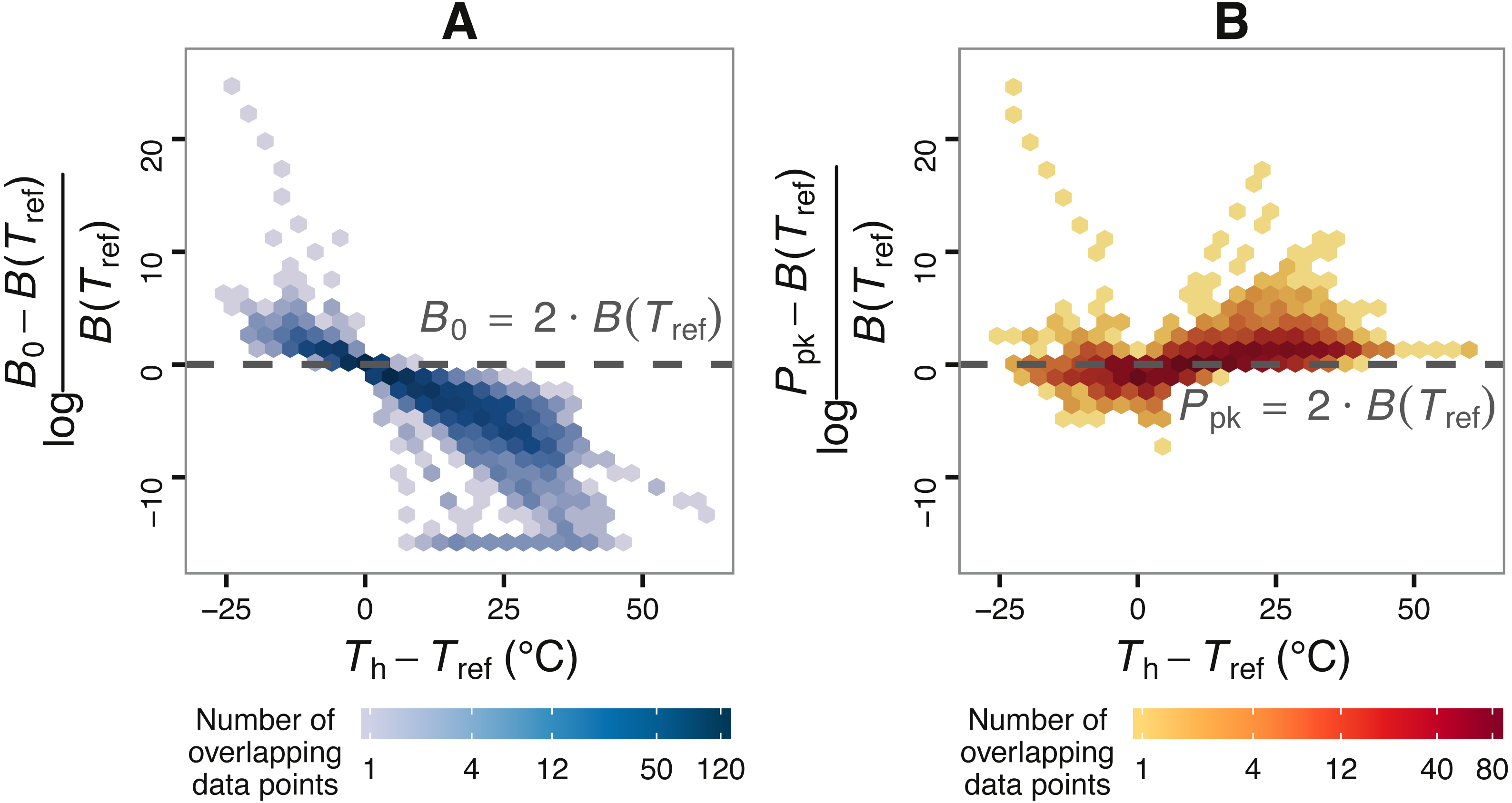

Download full-size image

DOI: 10.7717/peerj.4363/fig-2

Table 1:

Parameters for the generation of simulated curves.

α and β are shape parameters of the beta distribution, whereas the two other parameters generate variation in the width and the height of the curves. β is constrained to be smaller than α, in order for the resulting curves to be negatively skewed, similarly to the observed thermal response curves of biological rates.

Parameter name	Estimation
α	$α \sim N (μ = 10, σ = 3)$
β	α − i, $i \sim N (μ = 4, σ = 2)$
Final curve width	original width ⋅j, $j \sim N (μ = 25, σ = 4)$
Final curve height	original height +k, $k \sim N (μ = 3, σ = 0.8)$

DOI: 10.7717/peerj.4363/table-1

We then fitted the Sharpe-Schoolfield model to each synthetic curve and obtained parameter estimates where possible. Following this, we performed two different tests for MCA, and compared the results when using B₀ versus B(T_ref). For the first test, the estimates were split onto two groups: (i) those originating from curves with T_pk < 15 °C (colder-adapted species), and (ii) those with T_pk ≥ 15 °C (species adapted to warmer temperatures). We next tested whether the distributions of the normalised rates (B₀ and B(T_ref)) were significantly different using the two-sample Kolmogorov–Smirnov test (Corder & Foreman, 2014). The second test consisted of a simple correlation between the normalised rate values (B₀ and B(T_ref)) and the corresponding T_pk values.

Results

Conditions that lead to different degrees of inflation of B₀ estimates

Using the phytoplankton growth rates dataset, we show that, contingent on the difference between T_h and T_ref, B₀ can be considerably greater than B(T_ref) (Fig. 2). More precisely, the deviation of B₀ from B(T_ref) decreases nonlinearly with the difference between T_ref and T_h (A). In many circumstances, the deviation of B₀ is extreme, becoming even greater than the rate value at or near optimum temperature, P_pk (B).

The search for thermal response parameter combinations that lead to B₀ being above P_pk (highly overestimated) or below it (less overestimated) resulted in a conditional inference tree with four terminal nodes (Fig. 3). In each of those nodes, B₀ was nearly exclusively below or above P_pk. This machine learning model exhibited high performance both on the training dataset (MCC = 0.954) and the testing dataset (MCC = 0.824; section A3.2 in Appendix S1). The sets of thermal response parameters in which B₀ was greater than P_pk almost always had either a T_h − T_ref difference that was less than 0.6 (relatively narrow curves), or a T_pk − T_ref difference of 49.1 or lower (relatively wide curves).

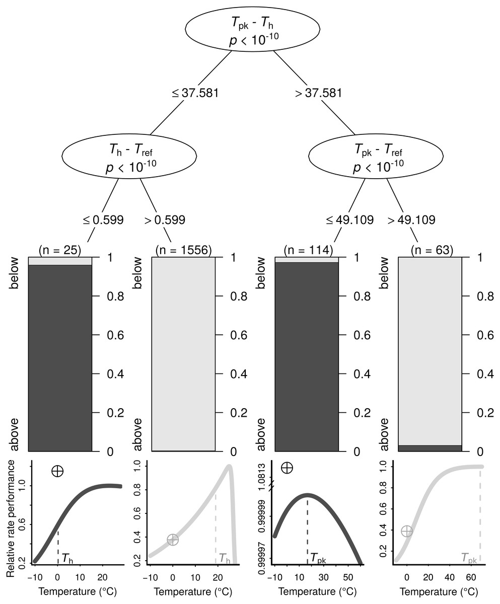
The conditions under which B0 is highly overestimated (i.e., B0 > Ppk; dark grey bars and curves) or less so (i.e., B0 < Ppk; light grey bars and curves), determined using a conditional inference tree algorithm. — Figure 3: The conditions under which B₀ is highly overestimated (i.e., B₀ > P_pk; dark grey bars and curves) or less so (i.e., B₀ < P_pk; light grey bars and curves), determined using a conditional inference tree algorithm.
Representative examples of thermal performance curves, along with their B₀ estimates (crossed circles; normalised at 0 °C for consistency), are shown under each terminal node. The curves are not drawn on the same axes, as their rate performance values vary considerably, even if normalised relatively to the P_pk value of each TPC. For a few very wide—and possibly biologically unrealistic—curves (right half), the difference between T_pk and T_ref determines whether B₀ > P_pk. In contrast, for the remaining curves, a T_h value that is greater than T_ref by more than 0.599 °C will always lead to B₀ estimates that are below P_pk.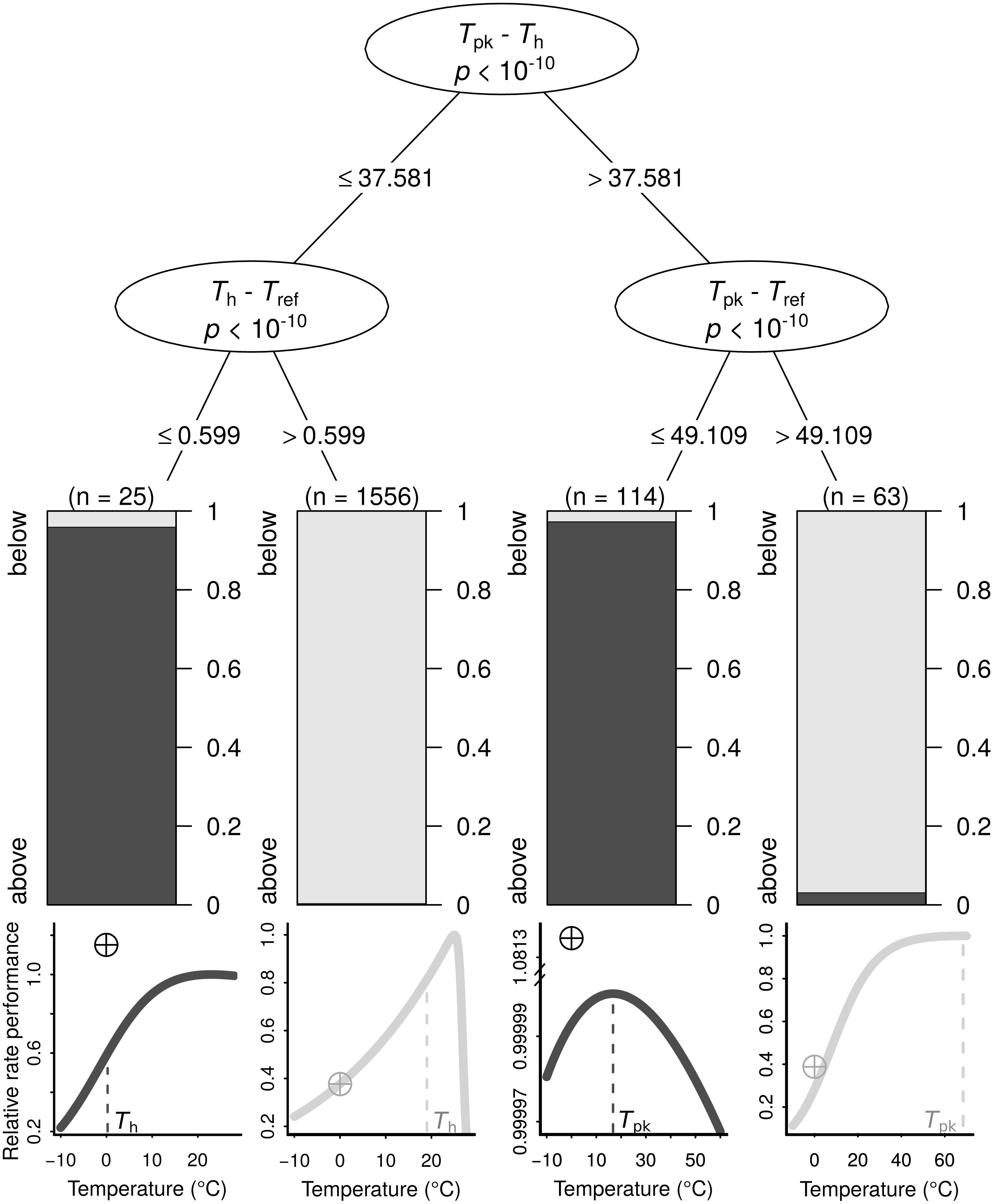

Download full-size image

DOI: 10.7717/peerj.4363/fig-3

Impacts of the overestimation of B₀ on tests for MCA

In total, we were able to obtain thermal response parameter estimates for 968 simulated curves, as the nonlinear least-squares algorithm failed to converge on solutions for the remaining 32. In the first test for MCA the distributions of B₀ estimates differed between the two groups (D = 0.18, p = 1.7⋅10⁻⁶), with species adapted to colder temperatures having a higher median value of B₀ (Fig. 4A, light blue violin plots). In contrast, the two distributions of B(T_ref) estimates were statistically indistinguishable (D = 0.07, p = 0.21), as expected (Fig. 4A, green violin plots). The overestimation of B₀ also affected the second MCA test, as a weak negative correlation between B₀ and T_pk was detected, but not between B(T_ref) and T_pk (Figs. 4B and 4C). These results indicate that the inflation of B₀ can provide false support for the MCA hypothesis, even for datasets with complete absence of this pattern.

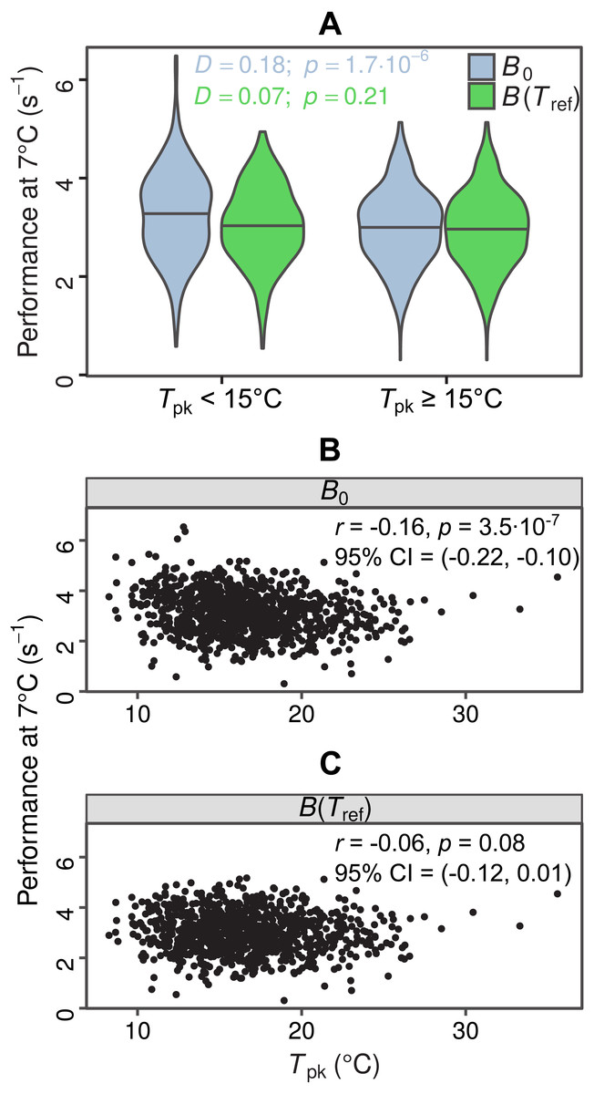
Impacts of exaggerated B0 estimates on tests for metabolic cold adaptation. — Figure 4: Impacts of exaggerated B₀ estimates on tests for metabolic cold adaptation.
(A) Violin plots of rate performance at T_ref = 7 °C, as estimated using B₀ (light blue) and B(T_ref) (green), for hypothetical cold-adapted species (T_pk < 15 °C; left half) and species adapted to higher temperatures (right half). Horizontal lines indicate the median of each distribution. The statistical significance of the difference in performance between the two temperature groups was evaluated according to the two-sample Kolmogorov–Smirnov test. Based purely on the B₀ estimates—which get increasingly inflated at low temperatures as T_h approaches T_ref—one would mistakenly conclude that metabolic cold adaptation is present in this dataset. (B, C): Correlations of B₀ with T_pk, and B(T_ref) with T_pk. The color surfaces represent the local density of data points. A similar pattern to the previous panel emerges, as the inflated B₀ estimates—in contrast to the true values—suggest that cold adaptation is present, albeit weakly.

Download full-size image

DOI: 10.7717/peerj.4363/fig-4

Discussion

In this paper we have addressed the consequences of estimating the value of a rate at a reference temperature, B₀, using the Sharpe-Schoolfield model, but without satisfying one of its fundamental assumptions: that the key enzyme—which is responsible for the temperature dependence of the rate—is fully functional at the reference temperature. When this assumption is not met, B₀ will overestimate the real rate performance at the reference temperature, B(T_ref) (Ikemoto, 2005).

We explain how the discrepancy between B₀ and B(T_ref) arises and determine the conditions under which it becomes particularly pronounced using a machine learning approach (Fig. 3). The resulting conditional inference tree shows that B₀ estimates will generally exceed the rate performance at the peak of the curve (P_pk) as long as: (i) T_pk − T_h is less than ∼37.58 °C and T_h − T_ref is less than ∼0.6 °C, or (ii) T_pk − T_h is greater than ∼37.58 °C and T_pk − T_ref is less than ∼49.11 °C. In any other case, B₀ would most likely be smaller than P_pk, although its inflation may well still be of concern. Using a synthetic dataset, we then demonstrate that wrongly assuming B₀ = B(T_ref) can lead to erroneous conclusions in analyses of thermal adaptation, as the overestimation of B₀ can mimic the effects of metabolic cold adaptation (Fig. 4) (a Type I error).

It is important to note that while we focus on the four-parameter version of the Sharpe-Schoolfield model in this study, the inflation of B₀ estimates also mathematically occurs in the variant of the model that assumes enzyme inactivation at both high and low temperatures. Thus, caution is warranted regardless of the model variant that is chosen. Beyond this issue, fitting the simpler model instead of its full counterpart may potentially give rise to other inherent biases but, to our knowledge, a thorough comparison of the two model variants across different organismal groups and rates is not available.

As mentioned before, previous studies have tended to set the T_ref—usually at a value of 25 °C—while fitting the Sharpe-Schoolfield model without considering the potential inflation of B₀ (Table A1 and Fig. A1, Appendix S1). Whether results of these studies have been compromised by an inappropriate use of T_ref is impossible to determine definitively because most of these studies report either T_h or T_pk estimates, whereas the machine learning model depends on both (see the ‘Conditions leading to a severely overestimated B₀’ section), along with the value of T_ref. If these data were available, using the machine learning model that we generated would provide a straightforward procedure to identify cases where B₀ is highly likely to be extremely overestimated (i.e, greater than P_pk). In fact, the only study where all necessary parameter estimates were reported for all fitted curves was that by Padfield et al. (2016). In that study, the maximum difference of T_h from T_pk is 2.49 °C, and the minimum difference of T_ref from T_h is 5.79 °C, which, according to the machine learning model (see Fig. 3), are sufficient for the B₀ estimates to be below those of P_pk. Having said that, as we showed in this paper, the fact that the overestimation of B₀ is not extreme does not necessarily rid any drawn conclusions of bias (e.g., the possibility of falsely detecting the effect of MCA).

In any case, it is crucial to point out that choosing an appropriate reference temperature (i.e., one that is low enough but within the temperature range that the species can endure) is not—on its own—a sufficient strategy to avoid the overestimation of B₀. As different species or individuals will most likely not share a common T_h value, the difference between T_h and T_ref will vary across the dataset (see Fig. 2). This approach could again lead to an exaggeration (which may however be very small) of some B₀ estimates and is therefore not an elegant solution to the problem.

Comparisons of temperature-normalised rates of diverse species

When data span the entire TPC

For studies in which the end goal is to compare the performance of different species at a common temperature, the simplest approach would be to fit the Sharpe-Schoolfield model—with or without normalising B₀ at a reference temperature—and compare estimates of B(T_ref), calculated a posteriori. The confidence intervals around B(T_ref) can then be estimated by bootstrapping. Another option to avoid the issue of rate overestimation is to consider fitting other models, such as the macromolecular rates model (Hobbs et al., 2013) or the enzyme-assisted Arrhenius model (DeLong et al., 2017).

When data only cover the rising part of the TPC

While the previous solutions are applicable to thermal response datasets that capture either the rise of the curve or its entirety, few studies report temperature performance measurements after the unimodal peak of the response (Dell, Pawar & Savage, 2011). Therefore, to obtain an estimate of baseline performance from a dataset that only covers the exponential rise component, one could instead fit the Boltzmann-Arrhenius model (e.g., see Gillooly et al., 2001), (3) $B (T) = B_{0} \cdot e^{\frac{- E}{k} \cdot (\frac{1}{T} - \frac{1}{T_{ref}})},$ which does not suffer from the problems of the Sharpe-Schoolfield model, as B(T_ref) indeed simplifies to B₀.

A second alternative model is the one that includes the Q₁₀ factor (see Gillooly et al., 2001), i.e., the rate of change in biological rate performance after a temperature rise of 10 °C: (4) $Q_{10} = {(\frac{B (T_{2})}{B (T_{1})})}^{\frac{10}{T_{2} - T_{1}}} .$ In this case, one would first estimate the value of Q₁₀ from known rate values at two temperatures, and use it to calculate the rate value at the reference temperature: (5) $B (T_{ref}) = B (T_{1}) \cdot Q_{10}^{\frac{T_{ref} - T_{1}}{10}} .$

Regardless of which of these two models is chosen, careful attention must be paid to ensure that the biological rate increases exponentially across the entire temperature range, without signs of a plateau being reached. Otherwise, the estimates may yet again be biased.

Using the ‘intrinsic optimum temperature’ instead of T_ref

Alternatively, baseline performance could be defined as the height of the curve at the temperature where the population of the key enzyme is fully active, which should be characteristic for each individual or species. In the Sharpe-Schoolfield model, the denominator indicates the percentage of enzymes that are active. Therefore, in the four-parameter variant of the model, the intrinsic optimum temperature could be estimated as the highest temperature at which this percentage is sufficiently high (e.g., at 99%). If, instead, the model of choice is the Sharpe-Schoolfield variant that also accounts for enzyme inactivation at low temperatures, there will be a unique temperature at which the enzyme population is 100% active. Otherwise, the intrinsic optimum temperature can also be obtained from the Sharpe-Schoolfield-Ikemoto (SSI) model (Ikemoto, 2005). This model integrates the law of total effective temperature—often used in studies of arthropod or parasite development—within the Sharpe-Schoolfield model, replacing T_ref with the intrinsic optimum temperature. However, this model introduces an extra parameter and is more challenging to fit compared to the original Sharpe-Schoolfield model. To mitigate this problem, software implementations have been developed that reduce the computation time from often more than 3 hours (Ikemoto, 2008) down to less than a second (Shi et al., 2011; Ikemoto, Kurahashi & Shi, 2013).

Conclusions

Obtaining accurate estimates of temperature-normalised rate performance is of crucial importance—especially in the face of climate change—for comparisons of the same rate across different organisms, or different rates within an individual. In this context, our study explains why temperature-normalised rate estimates obtained using the Sharpe-Schoolfield model can be strongly exaggerated—in comparison to the true rate values—when one of the assumptions of the model is violated, and gives an example of possible consequences of this exaggeration. The suggestions that we provide to address this issue should be useful to the burgeoning studies on ectotherm thermal performance and climate change, both for performing meta-analyses and for determining appropriate temperature ranges in laboratory experiments.

Supplemental Information

Supplementary material, mathematical derivations, and data sources

DOI: 10.7717/peerj.4363/supp-1

Download

Reliable Sharpe-Schoolfield parameter estimates across a range of Tref values

DOI: 10.7717/peerj.4363/supp-2

Download

Sharpe-Schoolfield parameter estimates, used for training the conditional inference tree

DOI: 10.7717/peerj.4363/supp-3

Download

Sharpe-Schoolfield parameter estimates, used for testing the conditional inference tree

DOI: 10.7717/peerj.4363/supp-4

Download

[1] Angilletta MJ. 2009. Thermal adaptation: a theoretical and empirical synthesis. Oxford: Oxford University Press.

[2] Angilletta MJ, Huey RB, Frazier MR. 2010. Thermodynamic effects on organismal performance: is hotter better? Physiological and Biochemical Zoology 83(2):197-206

[3] Angilletta MJ, Wilson RS, Navas CA, James RS. 2003. Tradeoffs and the evolution of thermal reaction norms. Trends in Ecology & Evolution 18(5):234-240

[4] Barmak DH, Dorso CO, Otero M, Solari HG. 2014. Modelling interventions during a dengue outbreak. Epidemiology and Infection 142(03):545-561

[5] Barneche DR, Kulbicki M, Floeter SR, Friedlander AM, Allen AP. 2016. Energetic and ecological constraints on population density of reef fishes. Proceedings of the Royal Society of London B: Biological Sciences 283(1823):20152186

[6] Barneche DR, Kulbicki M, Floeter SR, Friedlander AM, Maina J, Allen AP. 2014. Scaling metabolism from individuals to reef-fish communities at broad spatial scales. Ecology Letters 17(9):1067-1076

[7] Bissinger JE, Montagnes DJS, Sharples J, Atkinson D. 2008. Predicting marine phytoplankton maximum growth rates from temperature: improving on the Eppley curve using quantile regression. Limnology and Oceanography 53(2):487-493

[8] Brown JH, Gillooly JF, Allen AP, Savage VM, West GB. 2004. Toward a metabolic theory of ecology. Ecology 85(7):1771-1789

[9] Clarke A. 2004. Is there a universal temperature dependence of metabolism? Functional Ecology 18(2):252-256

[10] Clarke A. 2006. Temperature and the metabolic theory of ecology. Functional Ecology 20(2):405-412

[11] Clarke A. 2017. Principles of thermal ecology: temperature, energy, and life. Oxford University Press.

[12] Clarke A, Fraser KPP. 2004. Why does metabolism scale with temperature? Functional Ecology 18(2):243-251

[13] Corder GW, Foreman DI. 2014. Nonparametric statistics: a step-by-step approach (2nd Edition). Hoboken: John Wiley & Sons.

[14] Corkrey R, Olley J, Ratkowsky D, McMeekin T, Ross T. 2012. Universality of thermodynamic constants governing biological growth rates. PLOS ONE 7(2):e32003

[15] Dell AI, Pawar S, Savage VM. 2011. Systematic variation in the temperature dependence of physiological and ecological traits. Proceedings of the National Academy of Sciences of the United States of America 108(26):10591-10596

[16] Dell AI, Pawar S, Savage VM. 2013. The thermal dependence of biological traits. Ecology 94(5):1205-1206

[17] DeLong JP, Gibert JP, Luhring TM, Bachman G, Reed B, Neyer A, Montooth KL. 2017. The combined effects of reactant kinetics and enzyme stability explain the temperature dependence of metabolic rates. Ecology and Evolution 7(11):3940-3950

[18] Fand BB, Tonnang HEZ, Kumar M, Kamble AL, Bal SK. 2014. A temperature-based phenology model for predicting development, survival and population growth potential of the mealybug, Phenacoccus solenopsis Tinsley (Hemiptera: Pseudococcidae) Crop Protection 55:98-108

[19] Gillooly JF, Allen AP, Savage VM, Charnov EL, West GB, Brown JH. 2006. Response to Clarke and Fraser: effects of temperature on metabolic rate. Functional Ecology 20(2):400-404

[20] Gillooly JF, Brown JH, West GB, Savage VM, Charnov EL. 2001. Effects of size and temperature on metabolic rate. Science 293(5538):2248-2251

[21] Hobbs JK, Jiao W, Easter AD, Parker EJ, Schipper LA, Arcus VL. 2013. Change in heat capacity for enzyme catalysis determines temperature dependence of enzyme catalyzed rates. ACS Chemical Biology 8(11):2388-2393

[22] Hochachka PW, Somero GN. 2002. Biochemical adaptation: mechanism and process in physiological evolution. Oxford: Oxford University Press.

[23] Hoffmann AA, Sgrò CM. 2011. Climate change and evolutionary adaptation. Nature 470(7335):479-485

[24] Hopp MJ, Foley JA. 2001. Global-scale relationships between climate and the dengue fever vector, Aedes aegypti. Climatic Change 48(2–3):441-463

[25] Hothorn T, Hornik K, Zeileis A. 2006. Unbiased recursive partitioning: a conditional inference framework. Journal of Computational and Graphical Statistics 15(3):651-674

[26] Huey RB, Kingsolver JG. 1989. Evolution of thermal sensitivity of ectotherm performance. Trends in Ecology & Evolution 4(5):131-135

[27] Ikemoto T. 2005. Intrinsic optimum temperature for development of insects and mites. Environmental Entomology 34(6):1377-1387

[28] Ikemoto T. 2008. Tropical malaria does not mean hot environments. Journal of Medical Entomology 45(6):963-969

[29] Ikemoto T, Kurahashi I, Shi P-J. 2013. Confidence interval of intrinsic optimum temperature estimated using thermodynamic SSI model. Insect Science 20(3):420-428

[30] Johnson FH, Lewin I. 1946. The growth rate of E. coli in relation to temperature, quinine and coenzyme. Journal of Cellular and Comparative Physiology 28(1):47-75

[31] Johnson ZI, Zinser ER, Coe A, McNulty NP, Woodward EMS, Chisholm SW. 2006. Niche partitioning among Prochlorococcus ecotypes along ocean-scale environmental gradients. Science 311(5768):1737-1740

[32] López-Urrutia Á, San Martin E, Harris RP, Irigoien X. 2006. Scaling the metabolic balance of the oceans. Proceedings of the National Academy of Sciences of the United States of America 103(23):8739-8744

[33] Matthews BW. 1975. Comparison of the predicted and observed secondary structure of T4 phage lysozyme. Biochimica et Biophysica Acta (BBA)-Protein Structure 405(2):442-451

[34] Padfield D, Lowe C, Buckling A, Ffrench-Constant R, Student Research Team, Jennings S, Shelley F, Ólafsson JS, Yvon-Durocher G. 2017. Metabolic compensation constrains the temperature dependence of gross primary production. Ecology Letters 20(10):1250-1260

[35] Padfield D, Yvon-Durocher G, Buckling A, Jennings S, Yvon-Durocher G. 2016. Rapid evolution of metabolic traits explains thermal adaptation in phytoplankton. Ecology Letters 19(2):133-142

[36] Pawar S, Dell AI, Savage VM. 2015. From metabolic constraints on individuals to the dynamics of ecosystems. In: Belgrano A, Woodward G, Jacob U, eds. Aquatic functional biodiversity: an ecological and evolutionary perspective. London: Elsevier. 3-36

[37] Pawar S, Dell AI, Savage VM, Knies JL. 2016. Real versus artificial variation in the thermal sensitivity of biological traits. The American Naturalist 187(2):E41-E52

[38] Pörtner HO, Bennett AF, Bozinovic F, Clarke A, Lardies MA, Lucassen M, Pelster B, Schiemer F, Stillman JH. 2006. Trade-offs in thermal adaptation: the need for a molecular to ecological integration. Physiological and Biochemical Zoology 79(2):295-313

[39] Rose JM, Caron DA. 2007. Does low temperature constrain the growth rates of heterotrophic protists? Evidence and implications for algal blooms in cold waters. Limnology and Oceanography 52(2):886-895

[40] Schoolfield RM, Sharpe PJH, Magnuson CE. 1981. Non-linear regression of biological temperature-dependent rate models based on absolute reaction-rate theory. Journal of Theoretical Biology 88(4):719-731

[41] Schulte PM, Healy TM, Fangue NA. 2011. Thermal performance curves, phenotypic plasticity, and the time scales of temperature exposure. Integrative and Comparative Biology 51(5):691-702

[42] Seibel BA, Dymowska A, Rosenthal J. 2007. Metabolic temperature compensation and coevolution of locomotory performance in pteropod molluscs. Integrative and Comparative Biology 47(6):880-891

[43] Sharpe PJH, DeMichele DW. 1977. Reaction kinetics of poikilotherm development. Journal of Theoretical Biology 64(4):649-670

[44] Shi P, Ikemoto T, Egami C, Sun Y, Ge F. 2011. A modified program for estimating the parameters of the SSI model. Environmental Entomology 40(2):462-469

[45] Simoy MI, Simoy MV, Canziani GA. 2015. The effect of temperature on the population dynamics of Aedes aegypti. Ecological Modelling 314:100-110