Unsupervised inference approach to facial attractiveness

Description of the database

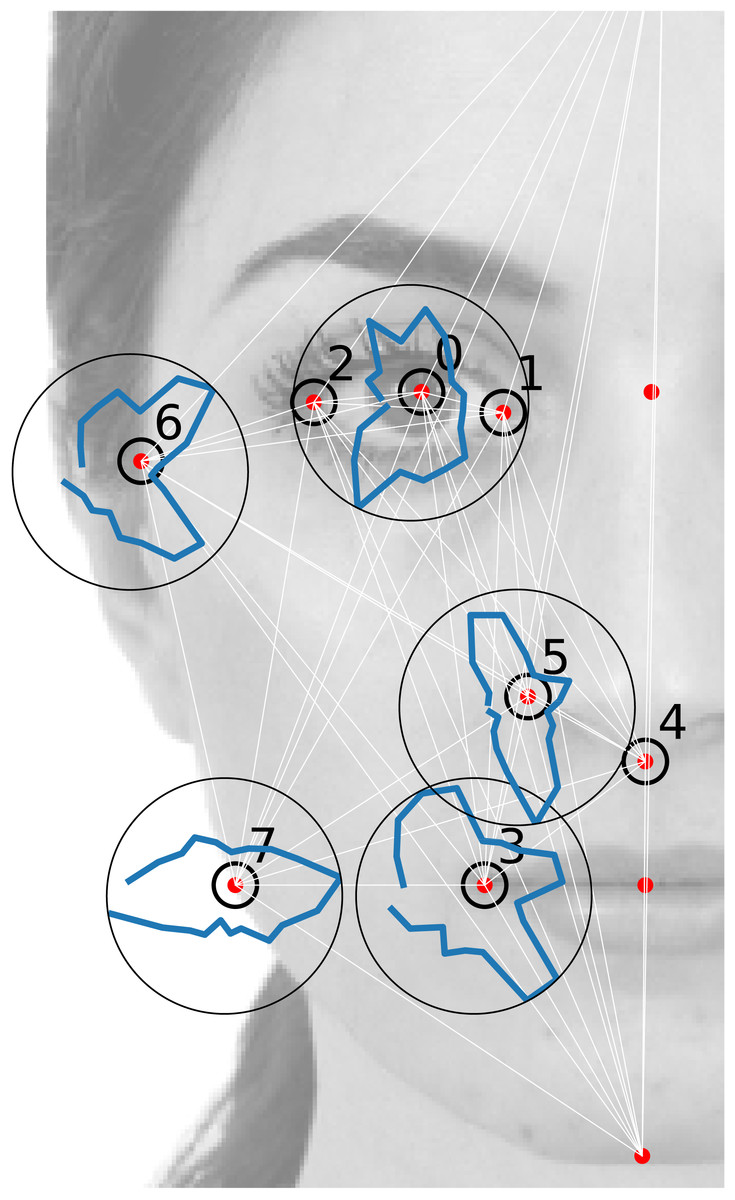
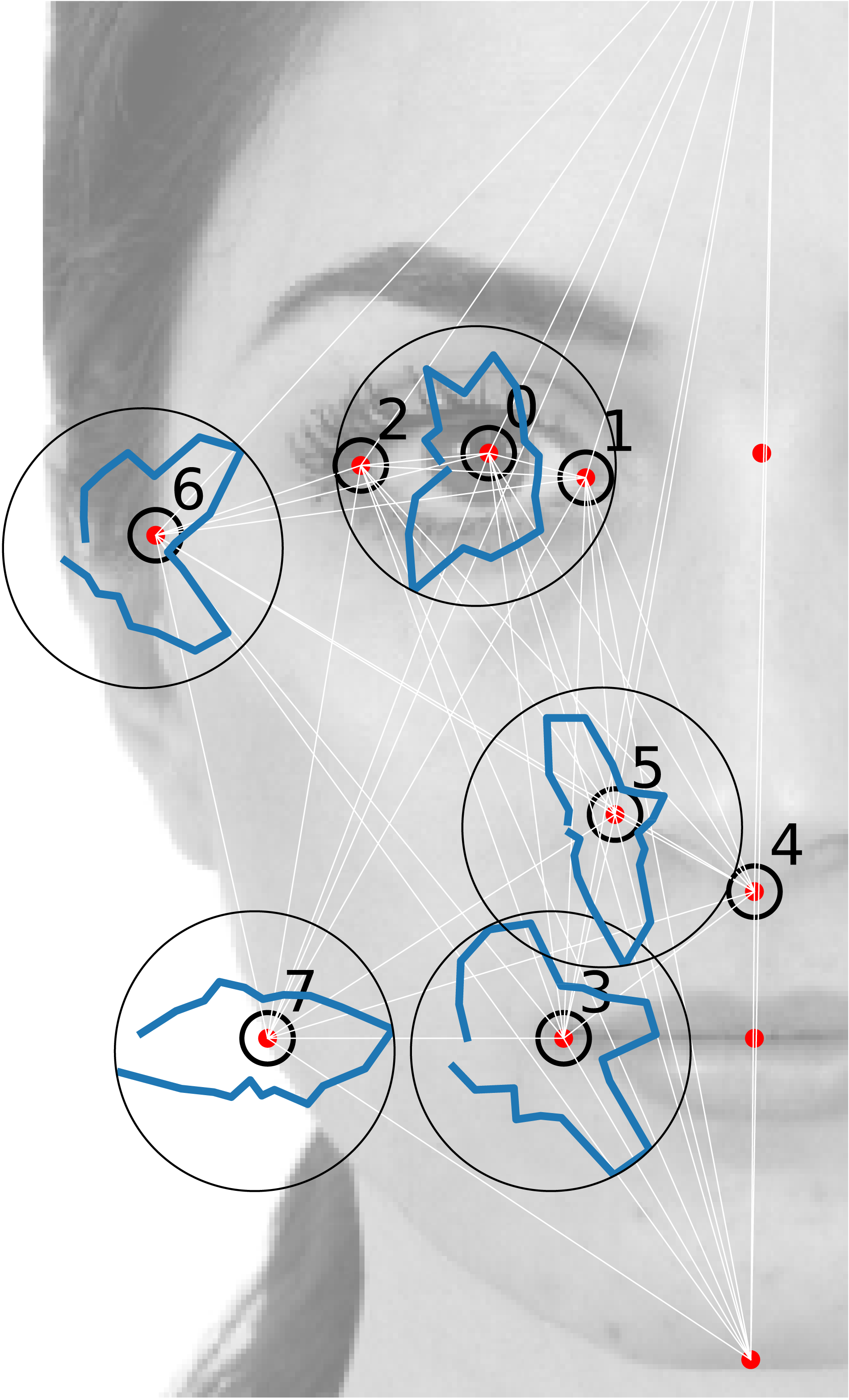
We analyse the dataset $\mathcal{S}$ described by Ibáñez-Berganza, Amico & Loreto (2019). In such experiments, each subject was allowed to sculpt her/his favorite deformation of a reference portrait (through the interaction with an software which combines image deformation techniques with a genetic algorithm for the efficient search in the face-space). The set of selected images are, hence, artificial, though completely realistic, variations of a common reference portrait (corresponding to a real person). In such a way, only the geometric positions of the landmarks are allowed to vary, the texture degrees of freedom are fixed (and correspond to the reference portrait RP1 (taken from the Chicago database, see (Ma, Correll & Wittenbrink (2015)) and Fig. 1). This representation of the face is, hence, rooted on a decoupling of geometric (also called shape) and texture (also called reflectance) degrees of freedom (Laurentini & Bottino, 2014).³ See Description of the E1 experiment in the Supplemental Information for a more detailed descriptions of the experimental protocol in Ibáñez-Berganza, Amico & Loreto (2019).

The database consists in the set of landmark geometric coordinates $\mathcal{S}={\left\{{\mathbf{r}}^{\left(s\right)}\right\}}_{s=1}^S$, where s is the facial vector index corresponding to the $\mathcal{N}=28$ vectors sculpted by each of the n_s = 95 experimental subjects (hence: $S=n_{\mathrm{s}}\mathcal{N}=\text{2,660}$).⁴ We will call ${\mathbf{r}}^{\left(s\right)}=\left(r_{\left(\mathsf{x},1\right)}^{\left(s\right)},\dots ,r_{\left(\mathsf{x},n\right)}^{\left(s\right)},r_{\left(\mathsf{y},1\right)}^{\left(s\right)},\dots ,r_{\left(\mathsf{y},n\right)}^{\left(s\right)}\right)$ the vector whose 2n components are the (x, y) Cartesian coordinates of a set of n = 8 landmarks, in units of the facial height. Such landmarks (those signaled with an empty circle in Fig. 1) are a subset of the set of landmarks used for the image deformation in Ibáñez-Berganza, Amico & Loreto (2019) (signaled with red points in Fig. 1). We will also refer to the 2D Cartesian vector of the ith landmark as ${\overrightarrow{r}}_i=\left({\mathsf{x}}_i,{\mathsf{y}}_i\right)$, and define the fluctuations of the landmark positions with respect to their average value as ${\overrightarrow{\Delta }}_i={\overrightarrow{r}}_i-〈{\overrightarrow{r}}_i〉$, where 〈⋅〉 denotes the experimental average, 〈⋅〉 = (1∕S)∑_s⋅. Analogously, Δ^(s) = r^(s) − 〈r〉. An important aspect of the dataset is that even the coordinates of the restricted set of n = 8 landmarks, r^(s), are redundant and depend on 10 coordinates only, due to the presence of 2n − 10 = 6 constraints that result from the very definition of the face-space. Such constraints are described in detail in the Supplemental Information.

Unsupervised inference

We now present some non-technical notion of unsupervised learning. In the next subsection we will describe the probabilistic models with which we describe the dataset. These are generative models that induce a likelihood probability density $\mathcal{L}\left(\cdot |\theta \right)$ over the space of facial vectors Δ. The meaning of $\mathcal{L}\left(\Delta |\theta \right)$ is that the probability of finding a facial vector in an interval of facial vectors I is given by ${\int }_{\mathbf{I}}\mathcal{L}\left(\Delta |\theta \right)\mathrm{d}\Delta$. The probabilistic model $\mathcal{L}$ represents a generalisation of the database, from which it is not unambiguously elicited. Indeed, a probabilistic model of the data depends both on the functional form of $\mathcal{L}$ (often called simply the model), and on the learning algorithm, or the protocol with which its parameters θ are inferred form the data.

For the learning algorithm, in the present work we adopt the Maximum Likelihood principle. We fix the parameters to the value that maximises the database likelihood: ${\theta }^{\ast }=arg{max}_{\theta }{\prod }_s\mathcal{L}\left({\Delta }^{\left(s\right)}|\theta \right)$, where the product is over all the samples in the database (please, see Inter- and intra-subject correlations and errors in the Supplemental Information for further information at this regard).

The functional form is given by the kind of unsupervised model. In this article we will consider three models (2- and 3-MaxEnt, GRBM), that will be described in the following subsections. The 2- and 3-MaxEnt models follows from the Maximum Entropy principle (Jaynes, 1957; Berg, 2017; Nguyen, Zecchina & Berg, 2017; Martino & Martino, 2018), which provides the functional form of the probability distribution $\mathcal{L}\left(\cdot |\theta \right)$ that exhibits maximum entropy and, at the same time, is consistent with the average experimental value of some observables of the data, 〈Σ〉, that will be called sufficient statistics. $\mathcal{L}$ must satisfy ${〈\Sigma 〉}_{\mathcal{L}}=〈\Sigma 〉$, where ${〈\cdot 〉}_{\mathcal{L}}$ refers to the expected value according to $\mathcal{L}$. In other words, $\mathcal{L}$ is the most general probability distributions constrained to exhibit a fixed expectation value of ${〈\Sigma 〉}_{\mathcal{L}}$ (and this value, under the Maximum Likelihood prescription, is given by the corresponding experimental value). The precise choice of the sufficient statistics determines the functional form of $\mathcal{L}\left(\Delta |\theta \right)$. A more detailed description is given in the next section and in section Introduction to the Maximum Entropy principle: correlations vs effective interactions of the Supplemental Information.

The maximum entropy models

We propose two MaxEnt probabilistic generative models of the set of selected faces, inferred from the dataset $\mathcal{S}$. In the case of the Gaussian or 2-MaxEnt model, the sufficient statistics is given by the 2n averages 〈Δ_μ〉 and by the 2n × 2n matrix of horizontal, vertical and oblique correlations among couples of vertical and horizontal landmark coordinates, whose components are C_μν = 〈Δ_μΔ_ν〉. In these equations, the 2n Greek indices μ = i, c_i denote the c_i = x, y coordinates of the ith landmark. The 2-MaxEnt model probability distribution takes the form (see Supplemental Information) of a Maxwell–Boltzmann distribution, $\mathcal{L}\left(\Delta |\theta \right)=\frac{1}{Z}exp\left(-H\left(\Delta |\theta \right)\right)$. In this equation, Z is a normalising constant (the partition function, in the language of statistical physics) depending on θ, and H = H₂ (the Hamiltonian) is the function: (1)${\displaystyle H_2\left(\Delta |{\theta }_2\right)=\frac{1}{2}{\Delta }^{†}\cdot J\cdot \Delta +{\mathbf{h}}^{†}\cdot \Delta .}$ The model depends on the parameters θ₂ = {J, h}, or the 2n × 2n matrix of effective interactions J and the 2n vector of effective fields, h. Due to the symmetry of matrix J, the number of independent parameters in the 2-MaxEnt model is D + D(D + 1)∕2, where D = 2n is the dimension of the vectors of landmark coordinates Δ. The value of these parameters is such that the equations $〈\Delta 〉={〈\Delta 〉}_{\mathcal{L}}$ and ${〈{\Delta }_{\mu }{\Delta }_{\nu }〉}_{\mathcal{L}}=C_{\mu \nu }$ are satisfied. This is equivalent to require that θ₂ are those that maximise the likelihood of the joint $\mathcal{L}$ over the database $\mathcal{S}$ (the Maximum Likelihood condition). The solution of such an inverse problem is (see Supplemental Information): J = C⁻¹, h = J⋅〈Δ〉, and Z = (2π)ⁿexp(h^†⋅J⁻¹⋅h∕2)(detJ)^−1∕2, where the −1 power in equation J = C⁻¹ denotes the pseudo-inverse operation, or the inverse matrix disregarding the null eigenvalues induced by the database constraints (see Supplemental Information). The 2-MaxEnt model is equivalent in the present case, in which the coordinates Δ_μ are real numbers, to a Principal Component Analysis and $\mathcal{L}$ is in this case a multi-variate Normal distribution.

We will define as well the 3-MaxEnt model. In this case, the sufficient statistics is given by averages 〈Δ_μ〉, pairwise correlations C_μν, and correlations among 3-landmark coordinates, $C_{\mu \nu \kappa }^{\left(3\right)}=〈{\Delta }_{\mu }{\Delta }_{\nu }{\Delta }_{\kappa }〉$. The 3-MaxEnt model probability distribution function takes the form of a Maxwell–Boltzmann distribution multiplied by a regularisation term ensuring that it is normalisable: (2)${\displaystyle \mathcal{L}\left(\cdot |\mathbf{h},J,Q\right)=\frac{1}{Z_3}{e}^{-\left[H_2\left(\cdot |{\theta }_2\right)+H_3\left(\cdot |Q\right)\right]}\mathsf{H}\left(\cdot |B\right)}$

where H(⋅|B) is a multivariate Heaviside function, equal to one for vectors Δ lying in the hypercube −B ≤ Δ_μ ≤ B for all µand zero otherwise; Z₃ is the normalising factor, and the Hamiltonian is H = H₂ + H₃, where H₂ given by Eq. (1) and H₃ by: (3)${\displaystyle H_3\left(\Delta |Q\right)=\frac{1}{6}\sum _{\mu \nu \kappa }{\Delta }_{\mu }{\Delta }_{\nu }{\Delta }_{\kappa }{Q}_{\mu \nu \kappa }}$ Besides h and J, the non-linear MaxEnt model depends on a further tensor of three-wise interaction constants among triplets of landmark coordinates. Consequently, the number of independent parameters is [D] + [D(D + 1)∕2] + [(D³ − D²)∕6 + D] = D³∕6 + D²∕3 + 5D∕2.

The solution of the inverse problem for the non-linear MaxEnt model does not take a closed analytic form. The maximum likelihood value of the parameters (h, J, Q) is numerically estimated by means of a deterministic gradient ascent algorithm (see Monechi, Ibáñez-Berganza & Loreto, 2020). A detailed explanation of the learning protocol may be found in the Supplemental Information (see Learning in the non-linear MaxEnt model). Before inferring the data with the non-linear models (3-MaxEnt and GRBM) we have eliminated a subset of 6 redundant coordinates from the original 2n coordinates. The data has been standardised in order to favor the likelihood maximisation process. The value of B has been chosen to be B = 6, so that the probability distribution function is nonzero only in an hypercube whose side is six times the standard deviation of each standardised variable.

The Restricted Boltzmann Machine model for unsupervised inference

We have learned the data with the (Gaussian-Binary) Restricted Boltzmann Machine (GRBM) model of unsupervised inference (Wang, Melchior & Wiskott, 2012; Wang, Melchior & Wiskott, 2014). It is a 2-layer unsupervised ANN, a variant, processing input real vectors, of the binary-binary RBM model. The model induces a probability distribution $\mathcal{L}\left(\Delta |\theta \right)={\sum }_{\mathbf{h}}p\left(\Delta ,\mathbf{h}|\theta \right)$ which is obtained by the marginalisation, over a set of N_h binary hidden variables (or hidden neurons), h_j ∈ {0, 1}, j = 1, …, N_h, of a joint probability distribution p: (4)${\displaystyle \mathcal{L}\left(\Delta |\theta \right)=\sum _{\mathbf{h}}p\left(\Delta ,\mathbf{h}|\theta \right),p\left(\mathbf{v},\mathbf{h}|\theta \right)=\frac{1}{Z_{\theta }}{e}^{-E\left(\mathbf{v},\mathbf{h}|\theta \right)}}$ The interaction among visible and hidden variables, and the dependence of p(Δ, h|θ) on all its arguments is described by an energy function E that couples hidden to visible neurons. E is defined in terms of a set of parameters θ consisting, among others, on the D × N_h matrix of synaptic weights among visible (input) and hidden variables. Although E presents only a linear coupling among v and h, the marginalisation over binary hidden neurons actually induce nonlinear effective couplings at all orders among the visible variables v (or Δ), couplings that may be accessed from the network parameters θ (MacKay, 2003; Cossu et al., 2019).

We have employed the open-source software (Melchior, 2017) for the efficient learning of GRBM. The learning protocol and parameters are described in detail, along with an introduction to the GRBM model, in the Supplemental Information, see: Learning the database with the Gaussian Restricted Boltzmann Machine.

Quality of the MaxEnt models as generative models

Histograms of single landmark-angle fluctuations

The quality of the 2-MaxEnt generative model as a faithful description of the database may be evaluated by the extent to what the model $\mathcal{L}$ reproduces observables O that it is not required to reproduce by construction. In other words, observables that cannot be written in terms of couples and triplets of coordinates Δ_α. The model is faithful in the extent to what $〈O〉\simeq {〈O〉}_{\mathcal{L}}$.

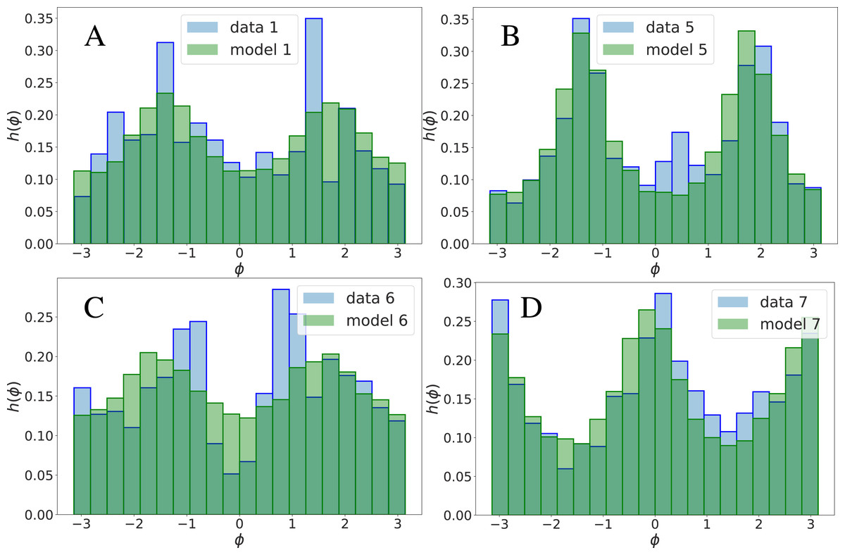
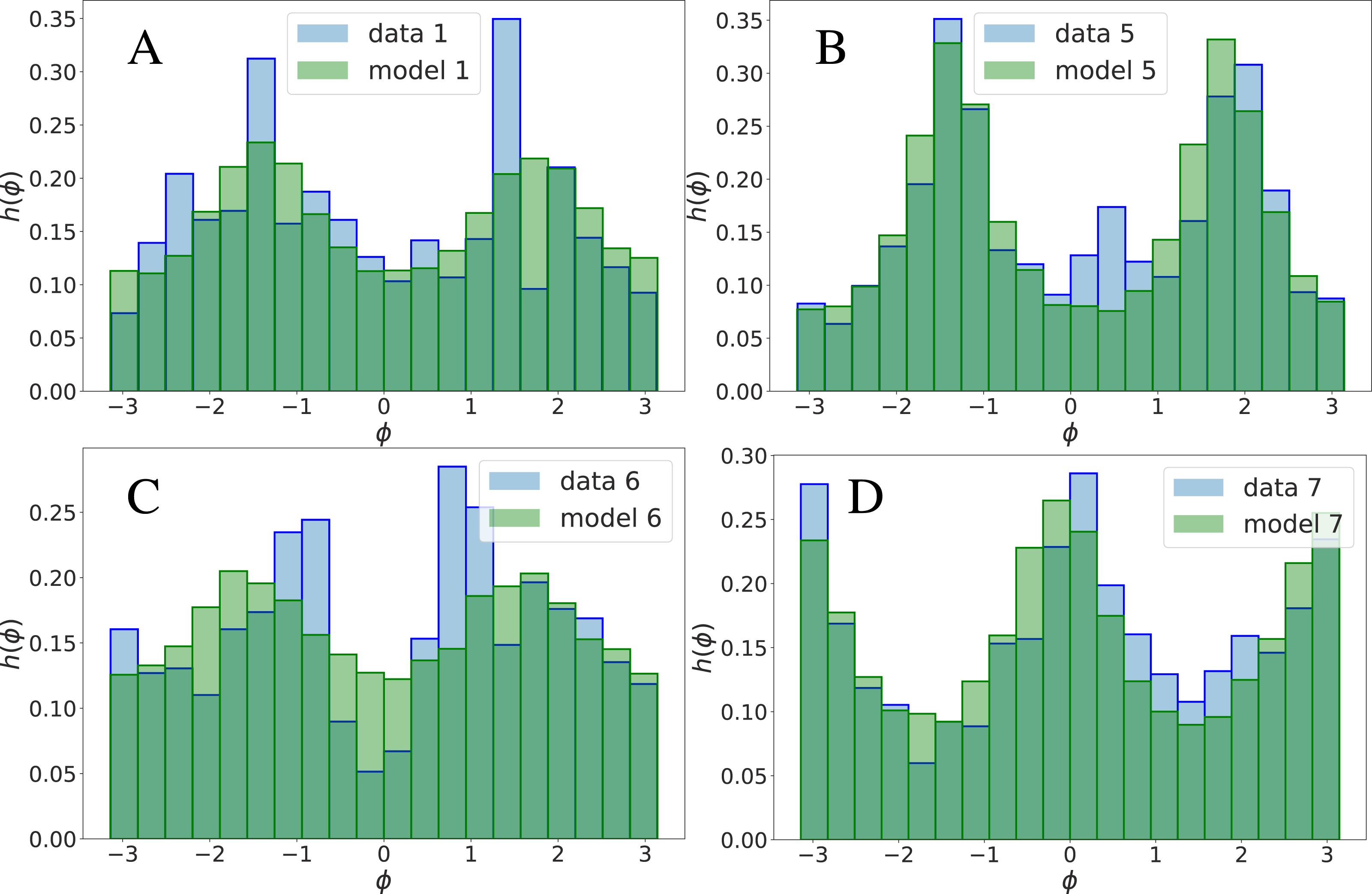
The ith landmark coordinates ${\overrightarrow{\Delta }}_i$ tend to fluctuate in the database with respect their average position $〈{\overrightarrow{\Delta }}_i〉=\overrightarrow{0}$. As a nonlinear observable O we will consider the angle that the ith landmark fluctuation ${\overrightarrow{\Delta }}_i$ forms with the x-axis. This quantity will be referred to as ${\varphi }_i^{\left(s\right)}=arctan\left({\Delta }_{i,\mathsf{y}}^{\left(s\right)}∕{\Delta }_{i,\mathsf{x}}^{\left(s\right)}\right)$. In Figs. 1 and 2, we report the empirical histogram of angles, h(ϕ_i) for some landmarks i. Remarkably, some landmarks’ angle distribution exhibit local maxima, probably reflecting their tendency to follow the direction of some inter-landmark segments (as it is apparent for the 3-rd and 6-th landmark’s in Fig. 1).⁵ We have compared the empirical histograms with the theoretical ϕ_i distributions according to the model. These have been obtained as the angle histograms of a set of S vectors Δ sampled from the inferred distribution $\mathcal{L}\left(\cdot |\theta \right)$ (see Fig. 2). The 2-MaxEnt model satisfactorily reproduces most of the landmark angle distributions. The empirical angle distribution, in other words, is reasonably well reproduced by the theoretical distribution $\mathsf{h}\left(\phi \right)=\int \mathrm{d}\Delta \mathcal{L}\left(\Delta |\theta \right)\delta \left(\varphi \left(\Delta \right)-\phi \right)$.

It is important to remark that the model-data agreement on h(ϕ_i) is observed also for large values of |ϕ_i| ∈ (0, π) (see Fig. 2), and not only for small values of |ϕ_i|, for which it approximately becomes |Δ_i,y∕Δ_i,x| (whose average is related to the correlation C_αβ, see Supplemental Information).

We conclude that, very remarkably, a highly non-linear observable as ϕ is well described by the 2-MaxEnt model, albeit it has been inferred from linear (pairwise) correlations only. In this sense, the 2-MaxEnt model is a faithful and economic description of the dataset. This picture is confirmed by the results of the following section which suggest, however, that a description of the gender differences in the dataset require taking into account effective interactions of order p > 2.

Performance of the MaxEnt model in a classification task

We now further evaluate the quality of the 2- and 3-MaxEnt models by assessing their efficiency to classify a test database of vectors in two disjoint subsets $\mathcal{S}={\mathcal{S}}_A\cup {\mathcal{S}}_B$ corresponding to the gender of the subject that sculpted the facial vector in Ibáñez-Berganza, Amico & Loreto (2019). We compare such efficiency with that of the GRBM model of ANN (see Wang, Melchior & Wiskott (2012) and Wang, Melchior & Wiskott (2014), ‘Materials and Methods’ and the Supplemental Information). This comparison allows to assess the relative relevance of products of p-facial coordinates Δ_α in the classification task: averages (p = 1), pairwise correlations (p = 2), and non-linear correlations of higher, p > 2 order (modelled by the 3-MaxEnt and GRBM models only).

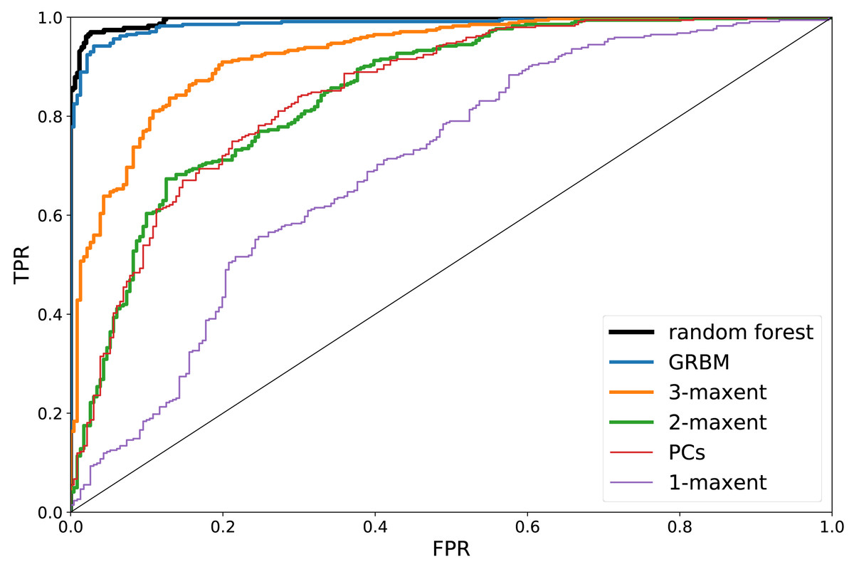
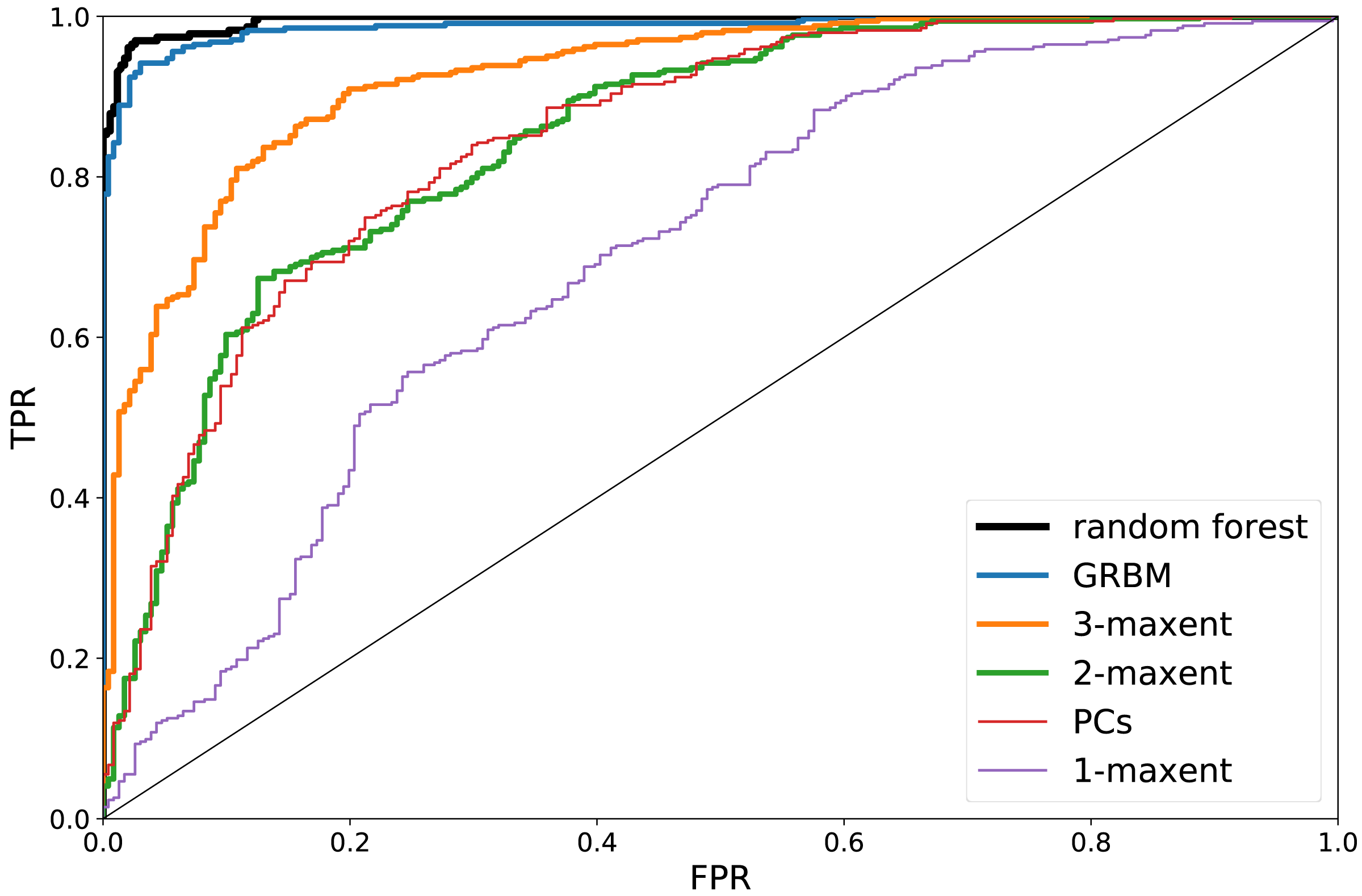
The dataset is divided in two disjoint classes ${\mathcal{S}}_A,{\mathcal{S}}_B$. Afterwards, both ${\mathcal{S}}_{A,B}$ are divided in training- and test- sets (20% and 80% of the elements of ${\mathcal{S}}_{A,B}$, respectively), and inferred the A and B training sets separately, with the MaxEnt and GRBM models. This results in six ({2, 3, G} × {A, B}) sets of parameters ${\theta }_{A,B}^{2,3,G}$, where the super-index refers to the model. Given a vector Δ belonging to the A or B test set, the score $\mathsf{s}\left(\Delta \right)=ln\mathcal{L}\left(\Delta |{\theta }_A\right)-ln\mathcal{L}\left(\Delta |{\theta }_B\right)$ is taken as the estimation of the model prediction for $\Delta \in {\mathcal{S}}_A$. The resulting Receiver Operating Characteristic (ROC) curves (Murphy, 2012) are shown in Fig. 3 for the various models considered.⁶

Considering only the averages 〈Δ〉 as sufficient statistics (or, equivalently, inferring only the fields h and setting $J_{ij}={\sigma }_i^{-2}{\delta }_{ij}$ in Eq. (1)) results in a poor, near-casual classification (specially in the most interesting region of the ROC curve, for small FPR and large TPR), see Fig. 3. The 2-MaxEnt model allows, indeed, for a more efficient classification. Rather remarkably, with the 3-MaxEnt and GRBM models the classification accuracy gradually increases. We interpret this as an indication of the fact that non-linear effective interactions at least of fourth order are necessary for a complete description of the database. For completeness, we have included a comparison with the Random Forest (RF) algorithm (Murphy, 2012). As shown in Fig. 3, RF achieves the highest classification accuracy (auRO C = 0.995, see Supplemental Information). We notice that this does not imply that the unsupervised models are less accurate: the RF algorithm is advantaged, being a specific model trained to classify at best the A, B partitions, not to provide a generative model of the A and B partitions separately.

We report the maximal accuracy scores for all the algorithms: RF (0.971); GRBM (0.952); 3-MaxEnt (0.865); 2-MaxEnt (0.764); 1-MaxEnt (0.680). The 2-MaxEnt model efficiency is, as expected, compatible with that of a t-Student test regarding the differences in the principal component values of A and B vectors, see Fig. 3. See the auROC scores of all the algorithms in the Supplemental Information.

We conclude that, on the one hand, the subjects’ gender strikingly determines her/his preferred set of faces, to such an extent that it may be predicted from the sculpted facial modification with an impressively high accuracy score (Murphy, 2012): a 97.1% of correct classifications. On the other hand, the relative efficiency of various models highlights the necessity of non-linear interactions for a description of the differences among male and female facial preference criterion in this database. Arguably, such nonlinear functions play also a role in the cognitive process of facial perception. The criterion with which the subjects evaluate and discriminate facial images seems to involve not only proportions r_α∕r_β (related to the pairwise correlations C_αβ, see Supplemental Information), but also triplets and quadruplets of facial coordinates influencing each other (yet, see the Supplemental Information for an alternative explanation).⁷

It is believed that the integration of different kinds of facial variables (geometric, feature-based versus texture, holistic, see Trigueros, Meng & Hartnett, 2018; Valentine, Lewis & Hills, 2016) improve the attractiveness inference results, suggesting that both kinds mutually influence each other in attractiveness (Eisenthal, Dror & Ruppin, 2006; Xu et al., 2017; Laurentini & Bottino, 2014; Ibáñez-Berganza, Amico & Loreto, 2019). The present results indicate that, even restricting to geometric coordinates (at fixed texture degrees of freedom), it is necessary a holistic approach, in the sense that it considers the mutual influence of many geometric coordinates.

Actually, our results indicate that pairwise influence of geometric coordinates are enough for a fair and economic description of the database (the 2-MaxEnt model predicts nonlinear observables, beyond the empirical information with which it has been fed). However, the differences among the facial vectors sculpted by males and females are not only encoded in pairwise correlations among geometric coordinates. Facial vectors reveal the gender of the sculpting subject with almost certainty only when non-linear models are used.

Analysis of the matrix of effective interactions

We now show that the generative models may provide directly interpretable information. This is an advantage of the MaxEnt method, whose parameters, the effective interaction constants, may exhibit an interpretable significance. We prove, in particular, that at least the matrix of effective interactions J admits an interpretation in terms of “resistance” (elastic constant) of inter-landmark segment distances and angles to differ with respect to their average or preferred value.

The 2-MaxEnt model admits an immediate interpretation. The associated probability density $\mathcal{L}\left(\Delta |\theta \right)=exp\left(-H_2\left(\Delta |\theta \right)\right)∕Z$ formally coincides with a Maxwell–Boltzmann probability distribution of a set of n interacting particles in the plane (with positions ${\overrightarrow{\Delta }}_i$, i = 1, …, n), subject to the influence of a thermal bath at constant temperature. Each couple i, j of such fictitious set of particles interacts through an harmonic coupling that corresponds to a set of three effective, virtual springs with non-isotropic elastic constants, J^{(x x)}_ij, J^{(y y)}_ij, J^{(x y)}_ij corresponding (see Eq. (1)) to horizontal, vertical and oblique displacements, Δ_i,x − Δ_j,x, Δ_i,y − Δ_j,y, and Δ_i,x − Δ_j,y, respectively.

The inferred effective interactions are more easily interpretable if one considers, rather than their x x, y y and x y components, the longitudinal and torsion effective interactions, $J_{ij}^{\parallel }$ and $J_{ij}^{\perp }$, respectively. The longitudinal coupling $\left|J_{ij}^{\parallel }\right|$ may be understood (see the Supplemental Information for a precise definition) as the elastic constant corresponding to the virtual spring that anchors the inter- ij landmark distance to its average value, 〈r_ij〉 (where ${\overrightarrow{r}}_{ij}={\overrightarrow{r}}_j-{\overrightarrow{r}}_i$). In its turn, the torsion interaction $\left|J_{ij}^{\perp }\right|$ is the elastic constant related to fluctuations of ${\overrightarrow{r}}_{ij}$ along the direction normal to ${\overrightarrow{r}}_{ij}$ or, equivalently, to fluctuations of the ij-segment angle, with respect to its average value that we will call α_ij = arctan(〈r_ij,y〉∕〈r_ij,x〉).

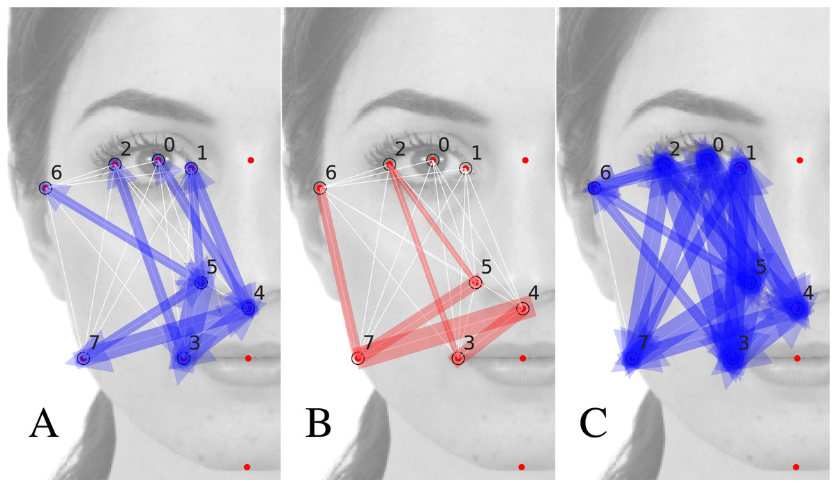
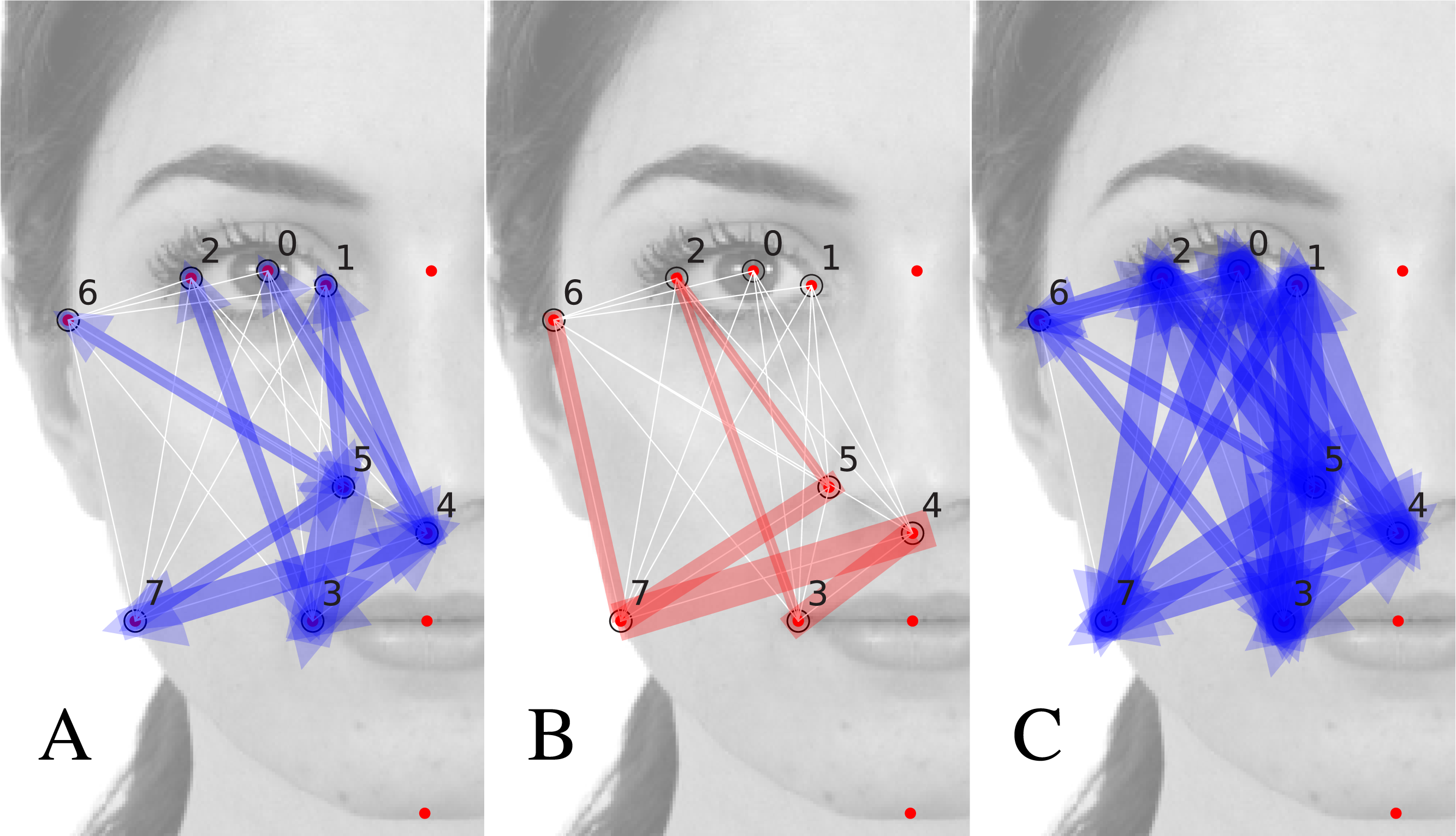
In Figs. 4A, 4B we show the quantities $\left|J_{ij}^{\parallel }\right|$ and $\left|J_{ij}^{\perp }\right|$ for those couples i, j presenting a statistically significant value (for which the t-value t_ij = |J_ij|∕σ_Jij > 1 (a description of the calculation protocol of the bootstrap error σ_ij may be found in the Supplemental Information). The width of the colored arrow over the i, j segment is proportional to $\left|J_{ij}^{\parallel }\right|$ (blue arrows in Fig. 4A) and $\left|J_{ij}^{\perp }\right|$ (red arrows in Fig. 4B). We notice that there exist inter-landmark segments for which $\left|J_{ij}^{\parallel }\right|$ is significant while $\left|J_{ij}^{\perp }\right|$ is not (as the 0, 4 or the 5, 6 segments) and vice-versa (as the 6, 7 and 2, 5). This suggests that $\left|J_{ij}^{\parallel }\right|$, $\left|J_{ij}^{\perp }\right|$ actually capture the cognitive relative relevance of distance fluctuations around 〈r_ij〉, and of angle fluctuations around α_ij.

We remark that the prominent importance of the inter-segment angles ij highlighted in Fig. 4B is fully compatible with the analysis presented in (Ibáñez-Berganza, Amico & Loreto, 2019) at the level of the oblique correlation matrix C^{(x y)}, and it goes beyond, as far as it quantitatively assess their relative relevance. As we will see in the next subsection, such information cannot be retrieved from the experimental matrix C only.

In the Supplemental Information we explain in more detail the analogy with the system of particles. We also analyse the dependence of the torsion and longitudinal effective interactions, $\left|J_{ij}^{\parallel }\right|$ and $\left|J_{ij}^{\perp }\right|$, with the average distance and angle of the ij inter-landmark segment, showing that there is a moderate decreasing trend of $\left|J_{ij}^{\parallel }\right|$ with 〈r_ij〉. This fact admits an interpretation: large inter-landmark distances are less “locked” to their preferred value with respect to shorter distances. Very interestingly, such trend is less evident for $\left|J_{ij}^{\perp }\right|$: the relative relevance of the inter-landmark angles according to J is not lower for farther away landmarks. This confirms the holistic nature of facial perception. The mutual influence among landmarks is not among nearby landmarks only, but over the scale of the entire face.