the Creative Commons Attribution 4.0 License.
the Creative Commons Attribution 4.0 License.
 | 12 Jan 2024
Field-data-based validation of an aero-servo-elastic solver for high-fidelity large-eddy simulations of industrial wind turbines
Etienne Muller
Simone Gremmo
Félix Houtin-Mongrolle
Bastien Duboc
Pierre Bénard
To design the next generations of wind turbines, engineers from the wind energy industry must now have access to new numerical tools, allowing the high-fidelity simulation of complex physical phenomena and thus a further calibration of lower-order models. For instance, the rotors of offshore wind turbines, whose diameters can now exceed 200 m, are highly flexible and fluid–structure interactions cannot be neglected any longer. Accordingly, this paper presents a new aero-servo-elastic solver designed to perform high-fidelity large-eddy simulation (LES) of wind turbines, as well as of rotor–wake interactions classically occurring in wind farms. In this framework, the turbine blades are modeled as flexible actuator lines. In terms of operating parameters (rotation speed and pitch angles) and power output, the solver is first validated against field data from the Westermost Rough offshore wind farm, for three different operation points. A very good agreement between the numerical results and field data is obtained. To push the validation further, additional results are compared to those given by a certified aero-servo-elastic solver used in the industry, which relies on a blade element momentum (BEM) method. The internal loads throughout the first blade and the deflections at the tip are studied in detail, and some discrepancies are observed. Of a reasonable amplitude overall, those are legitimately related to intrinsic modeling differences between the two solvers.
- Article
(15770 KB) - Full-text XML
- BibTeX
- EndNote


The aerodynamic high-fidelity simulation of an operating horizontal-axis wind turbine is challenging as it features a very high Reynolds number. Therefore one can expect a large range of spatial scales in the flow. Even today, despite the continuous growth of computational power, the direct numerical simulation of such a problem is still out of reach. In contrast, the large-eddy simulation (LES) approach is an interesting compromise to deal with this type of problem, especially when it comes to investigating the complex multi-scale physics of wind turbine wakes. Although mainly used in academic research, this approach is also attractive for the wind energy industry. Indeed, the results of LESs can complement partial field data when conducting the calibration, validation, and certification of low-order engineering models widely used in the industry. Such numerical results can also provide valuable insights into turbine–wake interactions at the scale of a wind farm. Understanding this phenomenon is indeed critical for siting engineers at the wake losses can significantly impact the annual energy production.
Yet, an LES can remain very costly depending on how the wind turbine is modeled. Using a full 3D model for the rotor, nacelle, and tower necessarily results in constraints on the cell size used in the vicinity of the walls and even more if the boundary layers developing in those regions are to be fully resolved. Regarding the authors' knowledge, the latter approach has only been reported by Lawson et al. (2019). In their work, the wall-resolved simulation of a National Renewable Energy Laboratory (NREL) 5 MW wind turbine was performed, for both laminar and turbulent inflows, on a grid counting more than 6 billion nodes. Noteworthy alternative approaches consist in hybrid LES–Reynolds-averaged Navier–Stokes (RANS) (detached-eddy simulation (DES) and derivatives) (Corson et al., 2012; Li et al., 2015; Thé and Yu, 2017) and wall-modeled techniques (Bénard et al., 2018), to achieve a lower time to solution. Still, simulating a whole wind farm using one of the aforementioned methods remains computationally unaffordable. This explains why the actuator line method (ALM), initially introduced by Sørensen and Shen (2002), is still a state-of-the-art approach to model a wind turbine at a reasonable cost in an LES framework. Originally, this method was designed to model the rotor blades as simple lines, discretized into 1D elements. The blade element theory is then used to compute the aerodynamic loads applied at the center of each element. The boundary layers around the blades are no longer resolved, thus considerably relaxing the constraints on the local cell size and avoiding the need to manage rotating or overlapping 3D meshes. To enhance the turbine representation, one can either add the tower and nacelle 3D geometries (Santoni et al., 2017; Ciri et al., 2017; Bénard et al., 2018) or model them as additional actuator lines/disks (Aitken et al., 2014; Churchfield et al., 2015; Gao et al., 2021; Stanly et al., 2022) to limit the extra computational cost.
The simulation of an operating wind turbine becomes even more challenging if one needs to predict the deflections of the blades. As a result, this aspect is still often overlooked in CFD (computational fluid dynamics) simulations reported in the literature. However, the latest offshore wind turbine prototypes have rotors whose diameters can exceed 200 m. By their composite structure and slenderness, the blades possess a degree of flexibility likely to induce fluid–structure interactions with the surrounding flow. Especially for a flexible blade, turbulent inflows can drastically increase the fluctuations over time of the aerodynamic coefficients and thus the fatigue (Rezaeiha et al., 2017).
To consider the structural response of a wind turbine to an incident flow, several cost-effective solvers have been designed in the wind energy community: OpenFAST (Jonkman and Buhl, 2005; National Renewable Energy Laboratory, 2022), HAWC2 (Larsen and Hansen, 2007), and BHawC (Rubak and Petersen, 2005), developed by NREL, the Technical University of Denmark (DTU), and Siemens Gamesa Renewable Energy (SGRE), respectively, are typical examples. All these solvers rely on the blade element momentum (BEM) method to compute the aerodynamic forces. Although predictive, these tools are limited by their inability to simulate the surrounding flow and especially the wakes. As such, one can no longer qualify these solvers as true CFD tools. To address the various design load cases (DLCs) referenced in the standards from the International Electrotechnical Commission (IEC), an appropriate modeling of the incoming flow, capturing the main physical mechanisms involved, is needed. For instance, assessing the loads experienced by a turbine operating in the wake of an upstream one is of critical importance. In such a scenario, the dynamic wake meandering (DWM) model, initially introduced by Larsen et al. (2007), can be used to mimic the dynamic of an incoming wake. Because they also feature a very low time to solution, these tools and wind models altogether are extensively used by wind turbine manufacturers to drive the design iterations or siting studies. Yet, careful calibrations of all models are needed for them to be certified and thus usable. This can be achieved by validating the predictions with field data and/or results from high-fidelity tools.
The latter, significantly more computationally intensive, mainly consist in a two-way coupling between a vortex-based or a CFD-like aerodynamic solver and a structural solver. The first one is in charge of getting the flow field, while the second one computes the structural response of the turbine. The literature already includes numerous works where this kind of approach is described (Lee et al., 2012; Li et al., 2015; Heinz et al., 2016; Dose et al., 2018; Meng et al., 2018; Sprague et al., 2020; Hodgson et al., 2021; Elie et al., 2022; Della Posta et al., 2022).
In this paper, we present the implementation and validation of a new solver derived from such a coupling: the high-order LES code YALES2 (Moureau et al., 2011) is used to solve the flow and compute the loads acting on the blades using the ALM, while the structural response is computed by BHawC (Rubak and Petersen, 2005). Besides, BHawC also allows us to embed the logic from the actual controller of industrial wind turbines. To the authors' best knowledge, for a coupling of the type described, the latter capability has only been reported in Gremmo et al. (2022). Still, it is worth mentioning that the external library used in this work to apply the controller logic was used as a black box in all simulations performed, as the authors never had access to the controller source code. In this study, the authors investigated a row of seven industrial wind turbines, operating in several wind conditions.
The paper is organized as follows. First of all, the two codes involved in the coupling are briefly described in Sect. 2, after which Sect. 3 presents thoroughly the coupling implementation. Finally, Sect. 4 presents the solver validation based on the simulation of an isolated turbine of the Westermost Rough offshore wind farm. Several operation points are considered in terms of wind speed and turbulence intensity. For each of them both YALES2 and YALES2–BHawC are used to model the wind turbine. The numerical predictions of the turbine overall performance are compared with field data. Additional numerical results, representative of the structural response, are also analyzed and compared in more depth.
2.1 YALES2: an aerodynamic solver
2.1.1 Governing equations
In the context of wind-energy-related LESs, one can solve the filtered Navier–Stokes equations for incompressible flows. Noting that ∼ represents the implicit spatial filtering resulting from the mesh resolution, these equations can be formally written as
where ν is the kinematic viscosity, the reduced pressure, and f a body force such as the gravity. The stress tensor τSGS results from the filtering operation and is a function of the unsolved sub-grid scales (SGSs) in the flow. In the present work, this tensor is assessed using the localized version of the dynamic model of Smagorinsky (Lilly, 1992).
2.1.2 Solver description
YALES2 (Moureau et al., 2011) is an in-house massively parallel finite-volume library intended for solving various fluid-mechanics-related problems. YALES2 includes, among other things, an incompressible solver for carrying out LESs of wind turbine wakes (Bénard et al., 2018).
When considering the equations given in Sect. 2.1.1, the pressure–velocity coupling is handled by a projection method (Chorin, 1968). In this framework, the Poisson equation for the pressure is solved with the deflated preconditioned conjugate gradient method reported in Malandain et al. (2013). Additionally, the solver makes use of a fourth-order two-step Runge–Kutta method to carry out the time integration. Likewise, the central scheme used for spatial discretization is fourth-order. To enhance the computing performance, an in-house two-level grid partitioning is used (Moureau et al., 2011). The first level consists in splitting the computational domain into partitions. A partition is a fraction of the computational domain, which is fully managed by one Message-Passing Interface (MPI) rank. Each partition is then further decomposed into a collection of cell groups. The number of cells included in each group is set to avoid any cache-memory miss.
2.1.3 Wind turbine modeling
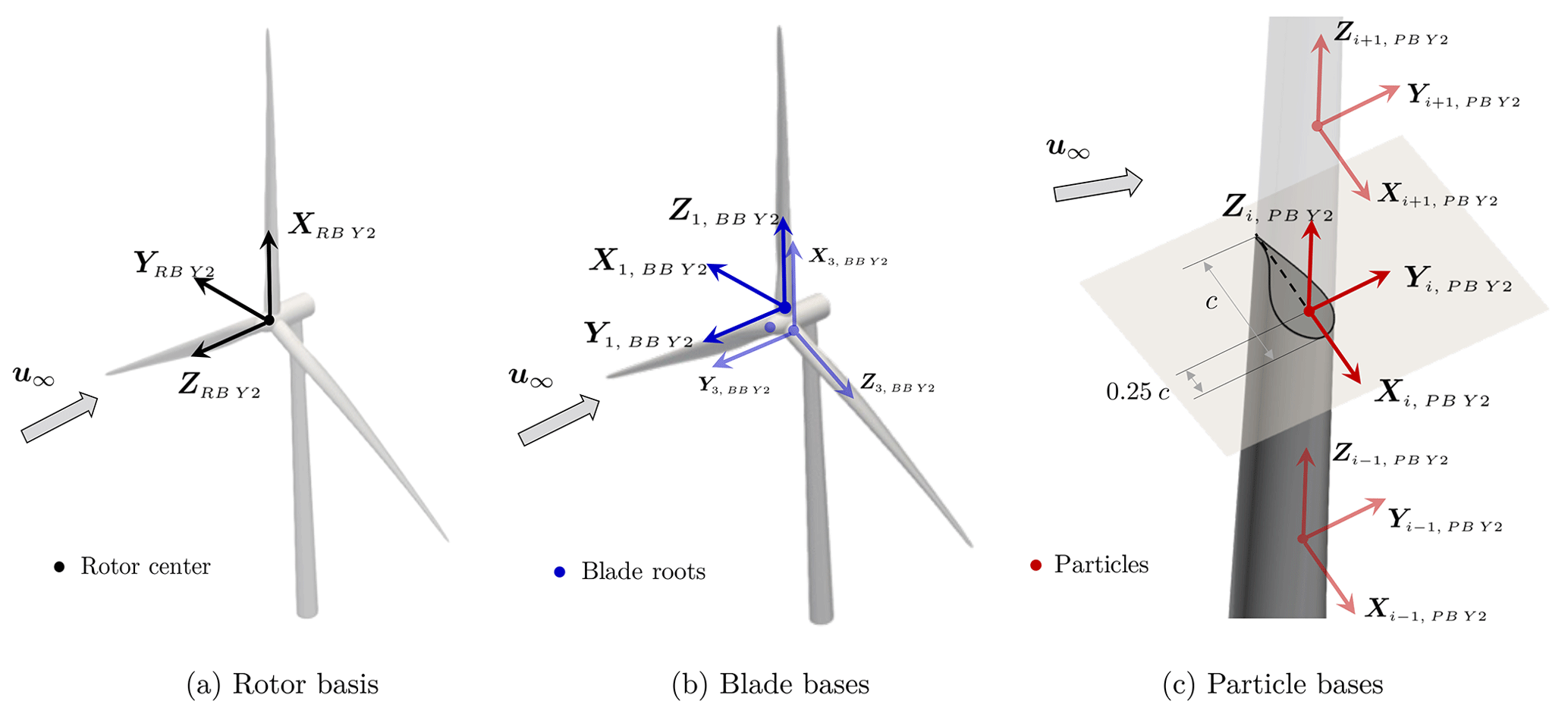
In YALES2, the ALM is used to model operating wind turbines. As stated in the Introduction, the approach allows us to model the forces applied by wind turbine blades on an incident flow. It is particularly suitable for investigating the physics of wind turbine wakes at a reasonable cost. Each blade geometry is replaced by a simple line, discretized into 1D elements of equal width w. The center point of an element is called the particle. The particle location is also chosen to match the quarter-chord point of the corresponding airfoil. In order to ease its handling, the rotor is simplified geometry relies on a set of 3D bases.
-
The rotor basis (RB). Linked to the rotor center, this basis allows us to represent the tilt and yaw angles. However, its orientation remains independent of the azimuthal rotation.
-
The blade bases (BB). Their origins coincide with the blade roots. They accurately translate the orientation of each blade, by taking into account their azimuthal position and the pitch angle. The turbine coning can also be represented by their means.
-
The particle bases (PB). They are attached to each blade element. They allow us to represent the local twist angle, as well as the prebend and sweep of the blades.
All these additional bases, illustrated in Fig. 1, are given in the global (GB) reference frame of YALES2 (Y2). For instance, the rotor basis can thus be written as the transition matrix . This natural framework proves very advantageous for navigating from one basis to another. Initially, the particle bases are linearly interpolated in a lookup table, which defines the blade undeformed geometry and contains similar bases associated with specific spanwise positions along the blade.
The lift L and drag D forces, assumed constant on each blade element, are computed at the particle location as follows:
where urel is the magnitude of the fluid velocity seen by the moving airfoil and ρ is the fluid density. The lift and drag coefficients, denoted CL and CD, respectively, here, are interpolated linearly in the aforementioned lookup table, which provides them as a function of both the angle of attack α and the spanwise position s along the blade. The airfoil chord c is also retrieved from the same lookup table. The velocity urel is further defined as a combination of both the local fluid velocity uf and the particle velocity :
Once given in the particle frame, this velocity enables us to compute the angle of attack α.
Yet, the forces obtained this way are singular and must be smoothed before being added as a body force in the Navier–Stokes equations. In the ALM framework, this operation is known as the mollification process. It acts as a spatial filtering operation, typically based on a Gaussian-like kernel η (Sørensen and Shen, 2002):
where d is the distance to the kernel center and ϵ is the kernel radius. The latter is usually chosen as twice the maximum cell size encountered in the rotor region.
For an exhaustive description of the ALM implementation in YALES2, the reader is referred to the PhD thesis of Houtin-Mongrolle (2022). Issues regarding the optimization of the ALM computational cost are also covered.
2.2 BHawC: an aero-servo-elastic solver
BHawC (Rubak and Petersen, 2005) is a nonlinear aero-servo-elastic solver intended to support the design and certification of wind turbines. Validated continuously against field data, the code allows a fast assessment of a wind turbine structural response to external loads so as to investigate numerous design load cases (DLCs) in a reasonable time. Indeed, for an appropriate discretization of the structure, the code can provide a 1:1 time to solution.1
A BHawC run can only handle one turbine at a time as it allows the definition of only one inflow. The assessment of the performance of a wind farm for given free-stream wind conditions, as well as the prediction of the loads applied to each individual turbine, remains feasible, provided that each BHawC instance relies on an appropriate inflow model (such as a DWM model). Nevertheless, all considered inflows are fully decoupled and thus possibly inconsistent.2
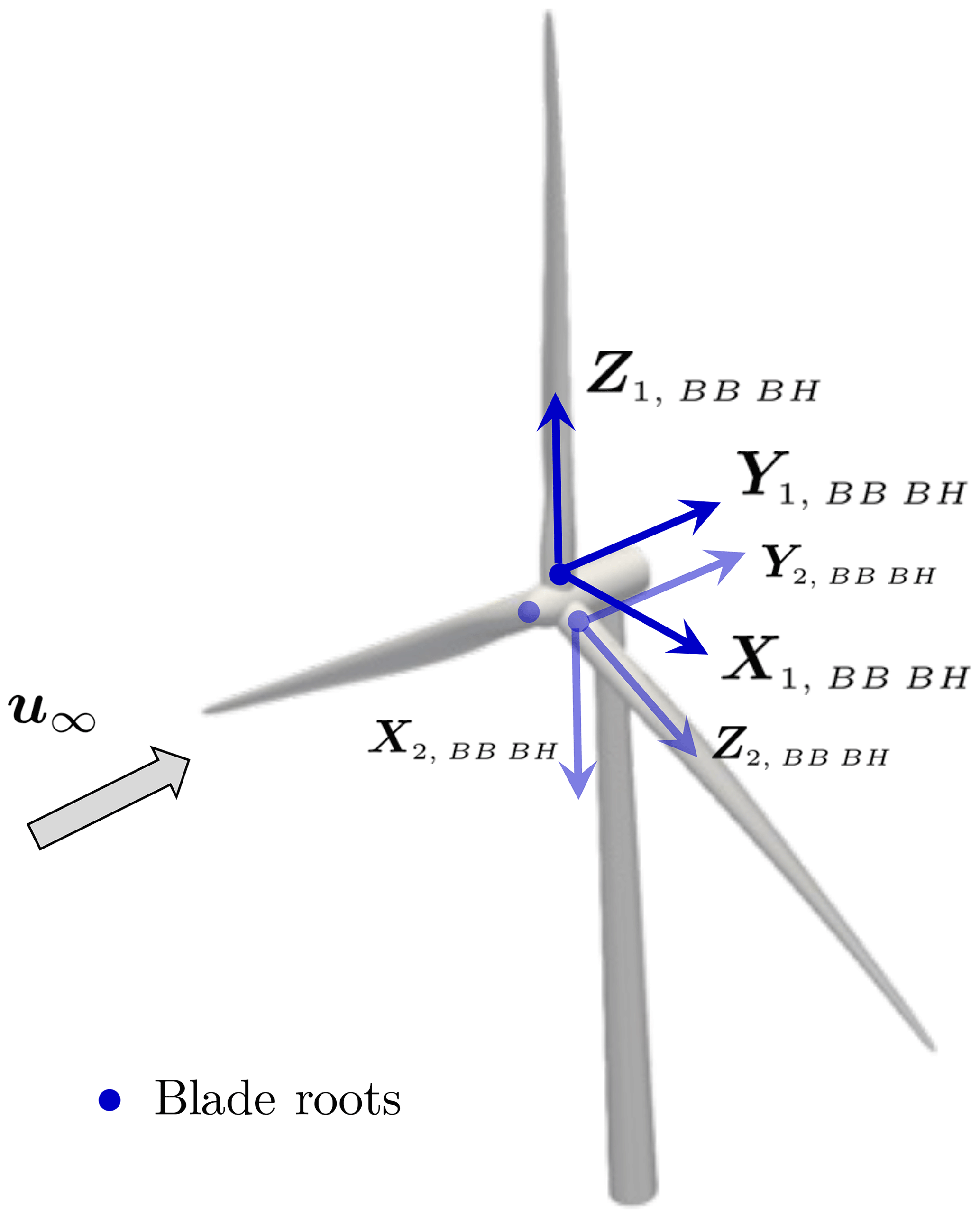
The modeling of a wind turbine consists of several sub-structures used to represent the foundation, tower, nacelle, hub, drivetrain, shafts, and rotor blades. Most of the sub-structures are modeled with equilibrium-based non-homogeneous anisotropic beam elements counting 12 degrees of freedom: three rotations and three translations per node (Krenk and Couturier, 2017). The drivetrain and the different bearings are modeled as purely torsional elements. Similarly to YALES2, BHawC also makes use of additional frames to manage the mentioned sub-structures and the elements used to discretize them. In particular, all the bases discussed in Sect. 2.1.3 have their twin in the BHawC (BH), even though their orientations can differ. This is the case for the blade bases, depicted in Fig. 2.
All the structural degrees of freedom, as well as their velocity and acceleration, are solved in BHawC (BH) global frame, which is attached to the bottom of the turbine foundation. The vector containing all the degrees of freedom is denoted by x(t) and its first and second derivative by and , respectively. BHawC targets the following equilibrium at each time step (Skjoldan, 2011):
where finer, fdamp, fint, and fext are the inertial, viscous damping, internal, and external loads, respectively. Especially the latter encompasses the aerodynamic loads. To solve the previous equation, the Newton–Raphson method is used to derive its residual form and iterate over it:
where M, C, and K are the mass, damping, and stiffness matrices, respectively. Additionally, the Newmark method is used to advance the system in time and relate and to x. This solution procedure leads to a linear system at each Newton iteration, where the correction vector δx is the only unknown. An LU factorization method is typically used to invert the system. Once δx is factored into x, the code updates the aforementioned matrices and all the components of the residual r except for the aerodynamic loads.
Those are computed only once per time step, prior to the first Newton iteration. To do so, BHawC relies on a blade element momentum (BEM) method (Sørensen, 2016), enhanced by many corrections. For instance, BHawC benefits from a modeling of the dynamic stall phenomenon (Leishman and Beddoes, 1989) and from the Prandtl correction for the tip/root losses, to cite only a few examples.
Finally, a complete framework is available in BHawC to include an emulation of a real controller in the wind turbine modeling. As a result, the rotor rotation speed is intrinsically unsteady. This approach also allows us to update other operating parameters in time, especially the pitch angles.
As implemented in YALES2, the ALM models the blades of a wind turbine as fully rigid lines, animated only by rotational movements. The azimuthal rotation speed is usually imposed as constant. This ALM implementation allows us to simulate the flow surrounding an arbitrary number of wind turbines. Phenomena such as wake steering, wake meandering, and wakes' combination can therefore be studied with YALES2. However, the structural response of a wind turbine to an incident flow remains unknown. Conversely, BHawC can provide the structural response of an industrial wind turbine, for a wide variety of incident flows, while also emulating real control strategies, meaning the azimuthal rotation speed is unsteady. Yet, the code does not offer any information on the resulting wake, and only one turbine can be handled at a time. In light of this, a coupling between YALES2 and BHawC was thus interesting to obtain accurate insights into the flow surrounding a turbine and the fluid–solid interactions involved when this turbine operates.
As designed, the coupling between YALES2 and BHawC only affects the blades of the wind turbine. The remaining sub-structures, such as the nacelle and the tower, are still represented in BHawC, but the aerodynamic loads they would normally experience are disabled. In the following, the coupling strategy is described in detail, as well as the mathematical framework upon which the coupling relies to transfer data between YALES2 and BHawC. Additional technical information regarding the coupling itself can be found in Appendix B.
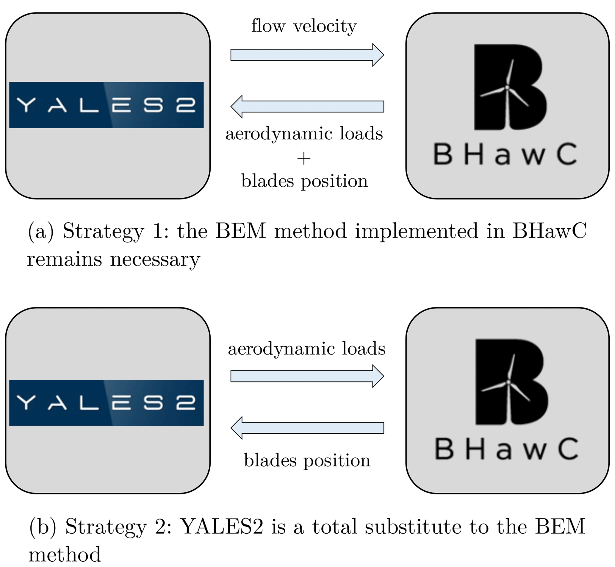
Figure 3Possible strategies to adopt for the coupling between YALES2 and BHawC. The second one was finally retained because it is more generic.
Regarding the coupling strategy, two options were available, which are depicted in Fig. 3. The first one is for instance employed in Lee et al. (2012), Sprague et al. (2020), Hodgson et al. (2021), and Elie et al. (2022). In this strategy, the structural solver (BHawC) first provides the position of the blade elements to the aerodynamic solver (YALES2), which can then assess the flow velocity at these positions. The flow velocity is returned to the structural solver and then combined with the blade elements' velocity to derive the relative velocity urel. The blade element theory, which is part of the BEM method, is then used to compute the aerodynamic loads acting on the blades. The loads contribute to the movement and deflections of the blades in the structural solver, but they are also sent back to the aerodynamic solver to be mollified on the Eulerian grid. From the authors' perspective, this approach is however not generic enough for several reasons. First, a standalone structural solver is not expected to compute external loads, as these are normally provided as inputs. In other words, this approach requires the structural solver to integrate a BEM module as well. Second, assuming that it is desired to also couple the tower and nacelle of the turbine, this strategy requires the structural solver to compute the loads acting on these sub-parts in the same way as for the blades, meaning by use of the blade element theory. Third, if the tower and nacelle were to be body-fitted in the aerodynamic solver, deriving the appropriate fluid velocities to send to the structural solver would not be straightforward anymore, as blockage effects would be fully represented in the vicinity of these sub-parts.
Given these limitations, the second coupling strategy was selected. In essence, BHawC communicates the current position and velocity of the blade elements to YALES2, and the ALM framework is used to compute and mollify the aerodynamic loads. The loads are also returned to BHawC to update the position and the deflections of the blades. One should note that this second approach completely bypasses the BEM method implemented in BHawC. This type of strategy is also used in Li et al. (2015) and Meng et al. (2018). In detail, the computation of the aerodynamic loads requires more information. In particular, the transition matrix must be known at each time step and for each blade element. This matrix represents the element bases, as given in the YALES2 global frame. It can be obtained as a chain of transition matrices:
Matrix (1) is computed only once as
The rotor deformations and rigid movements are managed directly in BHawC. This makes the rotor basis in YALES2 completely steady during the simulation. Thus, the second term on the right-hand side can be hard-coded. Matrices (2) and (3) are computed and sent by BHawC at every time step. Despite the particle bases in YALES2 (PB Y2) sharing the same overall orientation as those of the aerodynamic nodes in BHawC (PB BH), matrix (4) differs from the identity matrix. In a coupled simulation, the number of blade elements is enforced by YALES2 in order to guarantee their even distribution along the blade. This follows from the chosen mollification kernel (see Eq. 6), whose radius does not depend on the spanwise position. In this context, BHawC is unaware of the twist angle evolution along the blades and assumes it to be uniformly zero. In YALES2, the element bases remain set up as in a standalone simulation: their orientation therefore includes the twist angle. As the modeled airfoils are assumed to be fully rigid, this matrix is then computed only once as follows:
Like matrix (3), matrix (i) is computed and sent by BHawC. Matrix (ii) is trivially derived from Figs. 1 and 2, while matrix (iii) is interpolated from a lookup table (see Sect. 2.1.2).
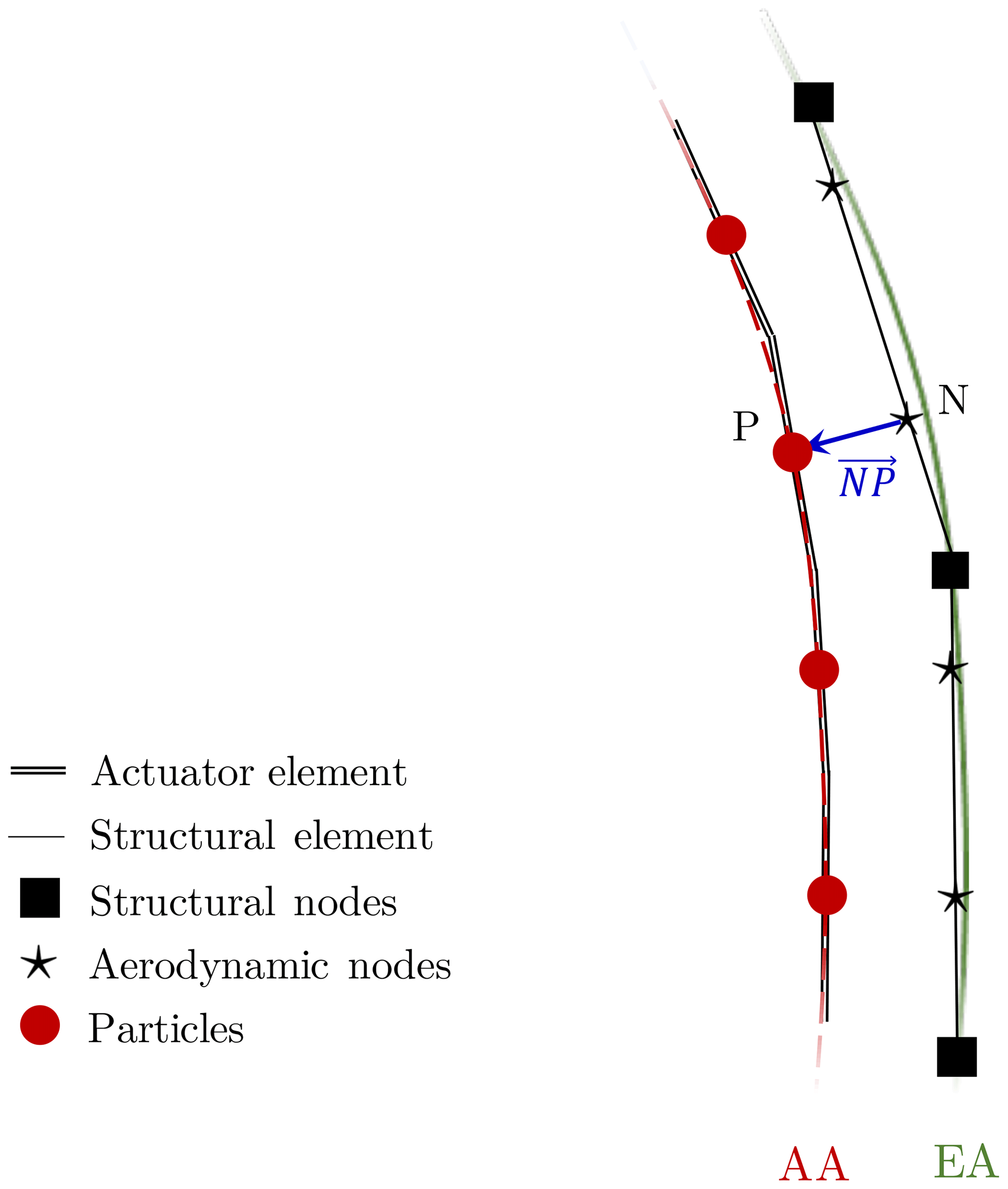
Figure 4Sketch of the blade discretization, illustrating the distinction between the aerodynamic axis (AA) and the elastic axis (EA).
The computation of the aerodynamic loads in YALES2 also requires obtaining the relative flow velocity at the particle position. As shown in Fig. 4, the particles are placed on a first axis, here called the aerodynamic axis (AA) for the sake of clarity. This axis differs from the elastic axis (EA) defined in BHawC, on which the corresponding aerodynamic nodes are located. Specifically, these nodes are positioned on the structural elements, which define the discretized elastic axis. During a coupled simulation, BHawC communicates to YALES2 the velocity and position of the aerodynamic nodes only. In that sense, the vector NP is needed for each blade element to (1) interpolate the fluid velocity at the particle actual position and (2) deduce the particle velocity from the one of the aerodynamic node:
where ΩGB Y2 is the rotation vector of the airfoil given in the YALES2 global frame.
As with the transition matrix , NP can be computed only once in the corresponding element basis, where it should remain constant afterwards. Once computed, the aerodynamic forces F and moments M are transferred back to the aerodynamic nodes and returned to BHawC. Here again, the vector NP is used to transport the moment from the AA to the EA:
At the beginning of each of its time steps, BHawC predicts the velocities and positions of the blade elements. The converged velocities and accelerations from the previous time step are used for this purpose. In addition, the next orientation of the element bases is also predicted. These data are then sent to YALES2. However the corresponding variables are not updated immediately so as to evaluate a relative velocity which accounts for the last mollification of the aerodynamic forces. Angles of attack are inferred using the element bases from the previous time step, and the aerodynamic loads are derived subsequently in these bases. The position, velocity, and basis of each element are then updated to transfer the loads into the global frame of both YALES2 and BHawC:
The forces FN,GB BH and moments MN,GB BH thus obtained are sent back to BHawC, and the iterative structural solver returns the next position and shape of each blade. The aerodynamic loads are kept constant in all Newton iterations to significantly speed up the simulation. This approximation is motivated by the small azimuthal angle swept by the blades during a time step. Meanwhile, the mollification of the forces takes place in YALES2, at the predicted position of the blade elements. The one or two iterations usually needed for the structural solver to converge warrant this second approximation. As previously described, the advancement of a blade is further illustrated in Fig. 5.
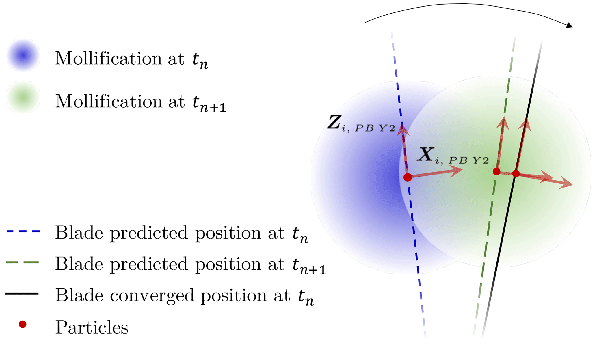
Figure 5Displacement of a blade portion during a time step. The predicted and final positions were made significantly different only for the sake of clarity, but in practice they almost overlap.
For an adequate trade-off between accuracy, stability, and time to solution, the time-step size commonly used in BHawC is ΔtBH=0.02 s. However, applying the CFL conditions (related to both the local fluid velocity and blade-element velocities) in YALES2 can provide significantly larger time steps, depending on the far-field wind speed and mesh used. Therefore, imposing ΔtY2=ΔtBH leads to a computational overhead in most cases. This motivated the development of a sub-stepping mechanism to circumvent this situation. Specifically, the time step in YALES2 is allowed to be a multiple of the one used in BHawC, within the limit of ΔtY2=3 ΔtBH for stability issues. In this context, the aerodynamic loads are computed only once, during the first sub-step. During the subsequent one(s), YALES2 uses the predicted element bases to update the loads' orientation, before sending them to BHawC. While BHawC corrects the blades' shape and position, YALES2 performs the mollification of the aerodynamic forces at the predicted location of the blade elements.
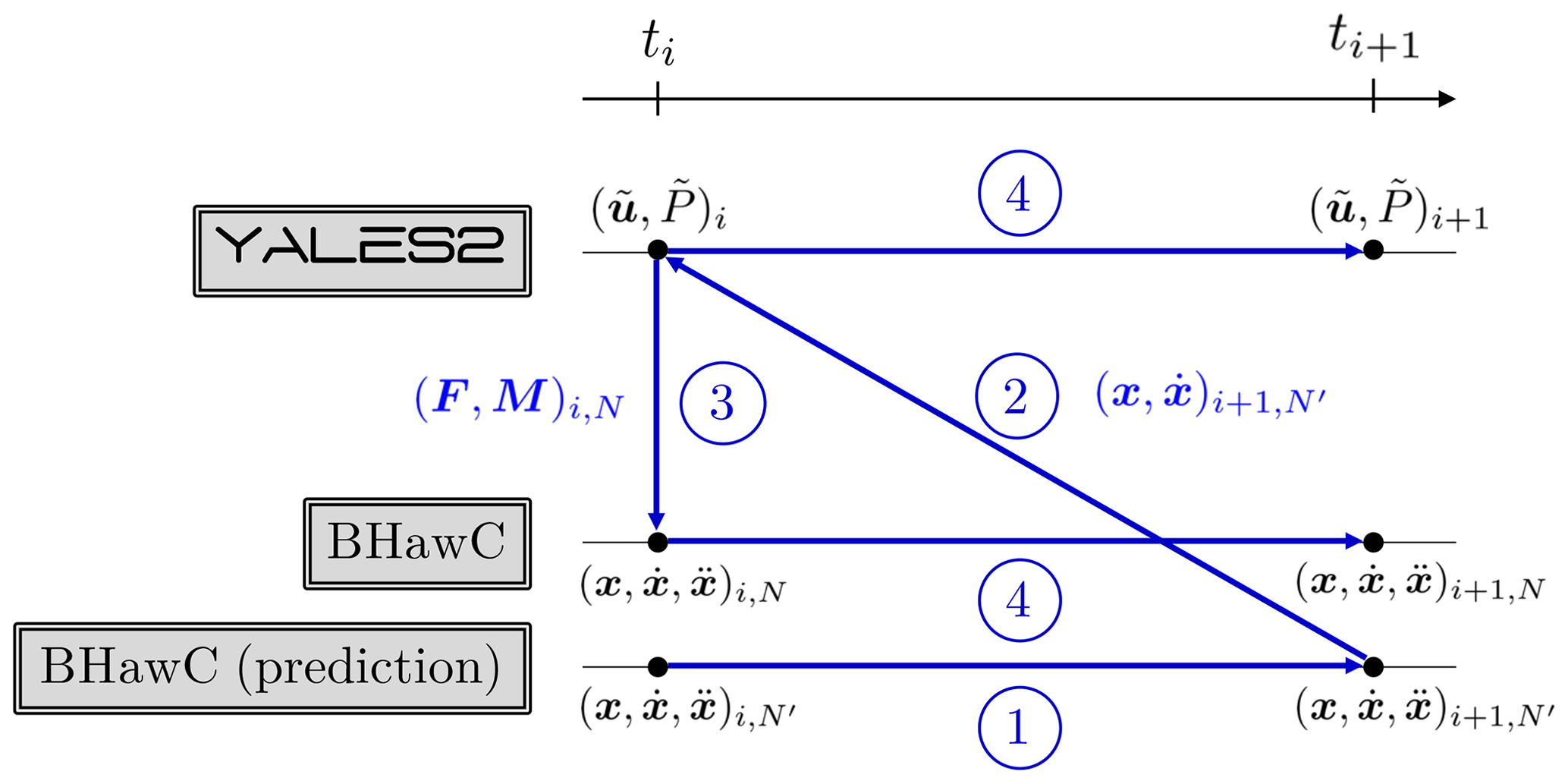
YALES2–BHawC is thus a partitioned loosely coupled solver. The coupling implementation is a combination of the conventional serial staggered (CSS) and conventional parallel staggered (CPS) procedures described by Farhat and Lesoinne (2000) (see Fig. 6). The CPS procedure aims at reducing the total computational cost of the coupled simulation by allowing the concurrent execution of the aerodynamic and structural solvers. However, its stability and accuracy require a sufficiently small time step (Farhat and Lesoinne, 2000). In the coupled simulations carried out, the structural solver occasionally diverged for wind speeds in the range from 8 to 12 m s−1 at hub height. We expect this issue to be at least partially removed by implementing an appropriate dynamic stall model in YALES2. Indeed, simulations carried out with the standalone version of BHawC (referred to in the text as “BHawC standalone”) showed a link between the divergence of the structural solver and the dynamic stall phenomenon model activation. It is emphasized that the induction is close to being maximum in the mentioned wind speed range, leading to a strong coupling between the structure and the ambient flow. Therefore, the relaxation of aerodynamic forces induced by the dynamic stall phenomenon is likely to be essential in these cases.
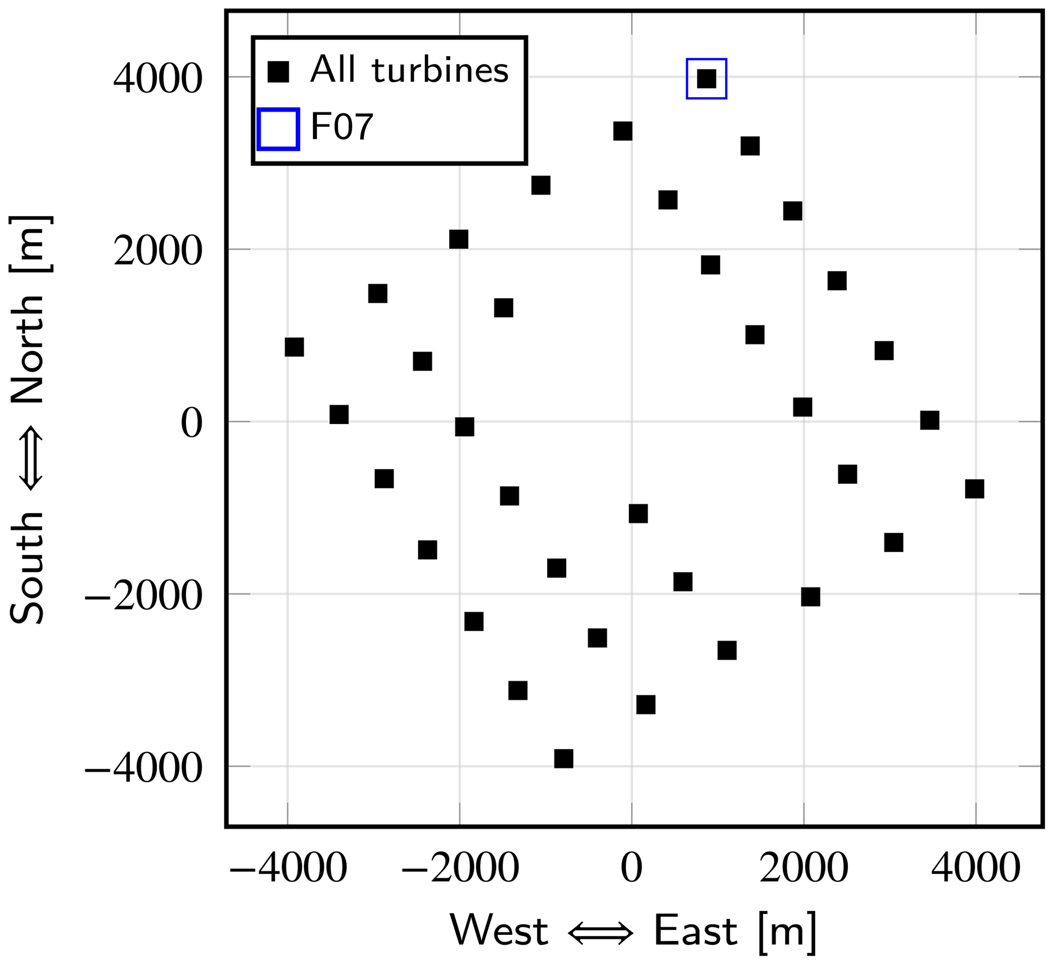
The validation of the coupled code YALES2–BHawC is carried out by considering the case of an isolated turbine of the Westermost Rough production site. This offshore wind farm, located near the Holderness coast of England, consists of 35 SWT-6.0-154 turbines (Siemens Gamesa Renewable Energy, 2014) for a covered area of 35 km2. The chosen turbine (whose identifier is F07) is highlighted with a blue square in Fig. 7, which also provides the rest of the wind farm layout. For a north wind, the turbine performance can be numerically predicted with YALES2–BHawC, without requiring any modeling of the neighboring turbines. Operating parameters obtained numerically are compared to field data, which derive from 10 min on-site recordings. To enhance the validation, BHawC standalone is also used to model the operating turbine. The deflections and internal loads of the blades obtained numerically are then compared in depth. Prior to this validation exercise, it should be emphasized that the coupling implementation has been thoroughly verified. Specifically, both the kinematic aspects (i.e., displacement/rotation of blade particles and attached bases) and the dynamic aspects (i.e., calculation and application of aerodynamic loads) were examined in detail. The related results are presented in Appendix A.
4.1 Numerical setups
The geometry of the computational domain used with YALES2 and the cell size mapping enforced within are provided in Fig. 8. The mesh counts 10 899 287 nodes and thus as many control volumes because YALES2 is node centered. The smallest cells are located in close vicinity to the turbine, and their size is set to to comply with the ALM common guidelines (Jha et al., 2014). The mesh size in the wake is however set to twice this value so that the whole mesh remains of reasonable size despite the domain extents. Close to the lower boundary, the mesh size is also set to to properly capture the stronger velocity gradient occurring in this region because of the wind shear.
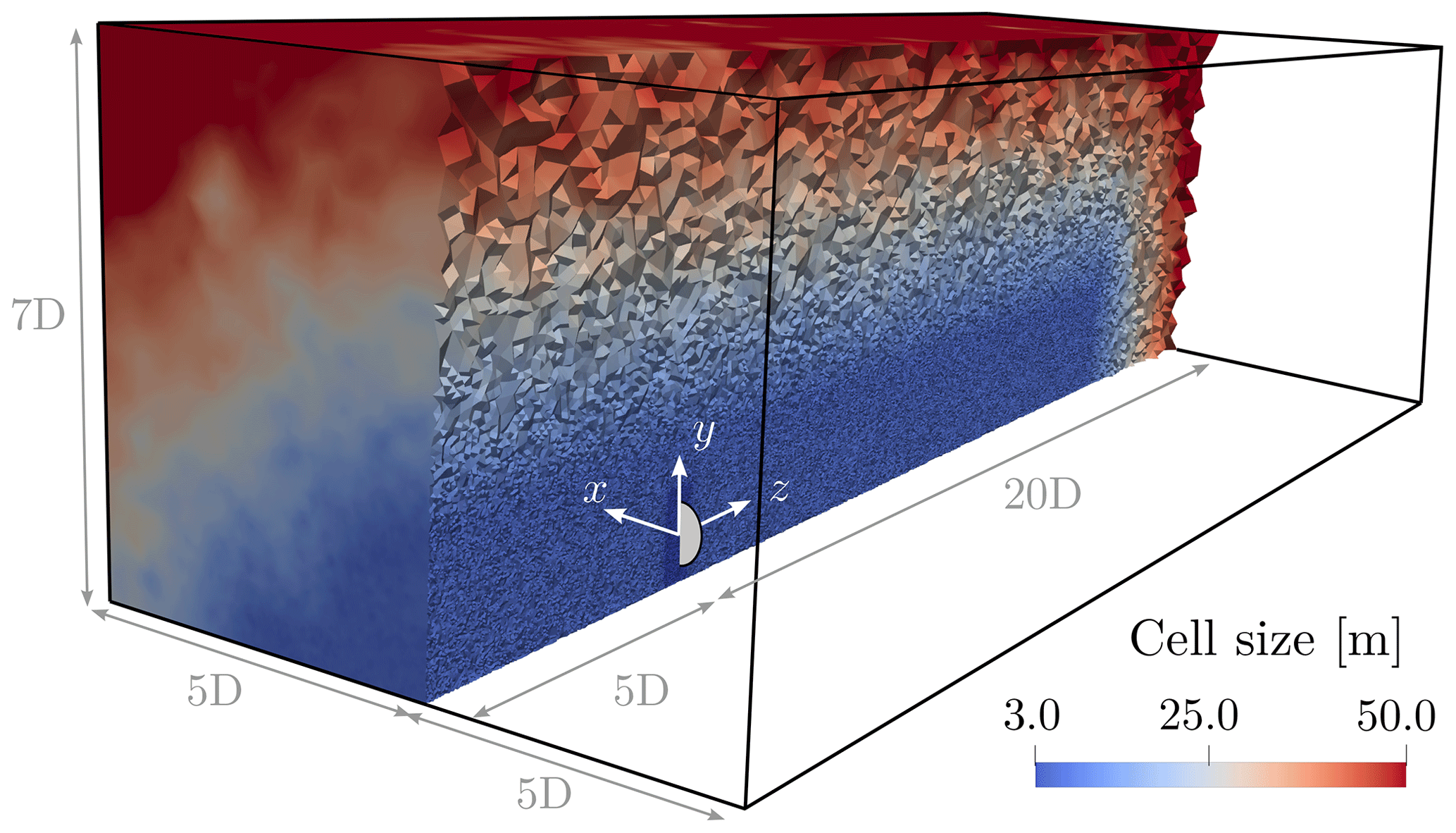
Figure 8Mesh and geometry of the computational domain used to investigate turbine F07 with YALES2–BHawC.
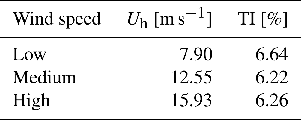
Regarding the boundary conditions, the lateral and upper surfaces are modeled as slipping walls. On the bottom surface, a classical logarithmic wall law including a roughness parameter is used to work around the full resolution of the atmospheric boundary layer. Due to the lack of reliable wind-assessment tools on the field, the inlet conditions result from a wind estimator. First, the recorded mean nacelle yaw angle is assumed to provide the wind direction. In the considered field data samples, the recorded mean yaw angles indicated a wind coming almost exactly from the north, with all deviations being below 1∘. Still, it should be noted that the standard deviations of the yaw angles were not zero, reaching 3.14∘ at most. This was deemed small enough to overlook the neighboring turbines' influence on the results. Second, the wind speed Uh and turbulence intensity at hub height are computed based on the power output and pitch angles of the turbine. In this study we consider three operating points, as given in Table 1. The inlet boundary condition is finally modeled as follows:
where denotes a synthetic turbulent velocity field based on the Mann model (Mann, 1994, 1998) and W(y) is the power law given by
The exponent α is set to 0.13, as this is a typical value for offshore applications (Burton et al., 2011). The velocity fluctuations are computed prior to the actual simulations, using the turbulence simulator from the International Electrotechnical Commission (IEC) (DTU Wind Energy, 2018), and then saved into periodic 3D boxes. Although anisotropic, this synthetic turbulence remains homogeneous, meaning for instance that the turbulence damping induced by the sea in the vertical direction is not factored in. The velocity field considered by BHawC in the BEM method is modeled identically.
Table 1Mean wind speeds and target turbulence intensities (TIs) at hub height on the inlet boundary.
As additional noteworthy parameters, the air density and kinematic viscosity are set to ρ=1.235 kg m−3 and m2 s−1, respectively. For simplicity's sake, we also enforce s in all simulations, thus putting aside the sub-stepping capability described in Sect. 3. For all considered wind speeds, this time-step size complies with the CFL conditions based on the flow velocity and the particle velocity.3
Concerning the turbine modeling, 75 evenly distributed aerodynamic nodes were used in BHawC to discretize each blade. Similarly, 75 particles were evenly distributed along each actuator line in YALES2–BHawC. This number was chosen to prevent interpolation errors when getting the aerodynamic coefficients from the blade lookup table. Indeed, 75 blade sections were referenced in the latter, which are at the exact same spanwise positions, respectively, as the defined aerodynamic nodes. The isotropic mollification kernels in YALES2 are defined with a radius . This choice was motivated by two main reasons. First this value, used along with a constant cell size in the rotor area, is widely used in the literature (Troldborg, 2009; Jha et al., 2014). Second, this work addresses the question of using LESs in an industrial context to further support improvements of lower-fidelity approaches, such as BEM-like methods or analytical wake models. The LES approach, from an industrial perspective at least, is still considered very costly due to the required CPU resources. Therefore, some trade-offs must be found between achievable accuracy and simulation cost. It is indeed shown in the literature that one should ideally opt for a varying value of ε along the blade span, to comply with the local length c of the blade section chord. The value of ε=0.25 c was for instance reported as a suitable choice (Shives and Crawford, 2013). Yet, as one must still comply with ε≥2Δgrid, the consistent mesh size in the rotor region would become prohibitive.
From a structural point of view, the blades are discretized with 19 beam elements of various lengths in order to achieve a suitable representation of the elastic-axis geometry at a reasonable cost. The nacelle and tower are not represented on the YALES2 side. Accordingly, the loads acting on them are forced to zero on the BHawC side, at all times. Regarding the wind turbine actual controller, it is emulated thanks to external libraries compiled beforehand.
4.2 Results
For confidentiality reasons, all the quantitative results shown in the current section are made nondimensional. Also, we first define the following operators:
where • is a quantity of interest, θN is defined as in Sect. A1, and T=600 s is a physical duration. These operators refer to azimuth-averaged and time-averaged results, respectively. We also introduce an additional discrete operator, referring to a mean value obtained at a given azimuth Θ:
For each wind speed considered, Fig. 9 starts by comparing the field data with the numerical results obtained with YALES2–BHawC and BHawC standalone, in terms of time-averaged rotation speed, pitch angle (first blade), and electrical power output. Overall, average values and standard deviations are well predicted with YALES2–BHawC for all the wind speeds of interest. The time-averaged values provided by BHawC appear to be almost the same as those given by the coupled code. However, one can observe meaningful differences in the standard deviations. Those obtained with BHawC standalone are up to 3 times lower than those given by the coupled code. This is especially visible for the rotation speed at low wind speed.
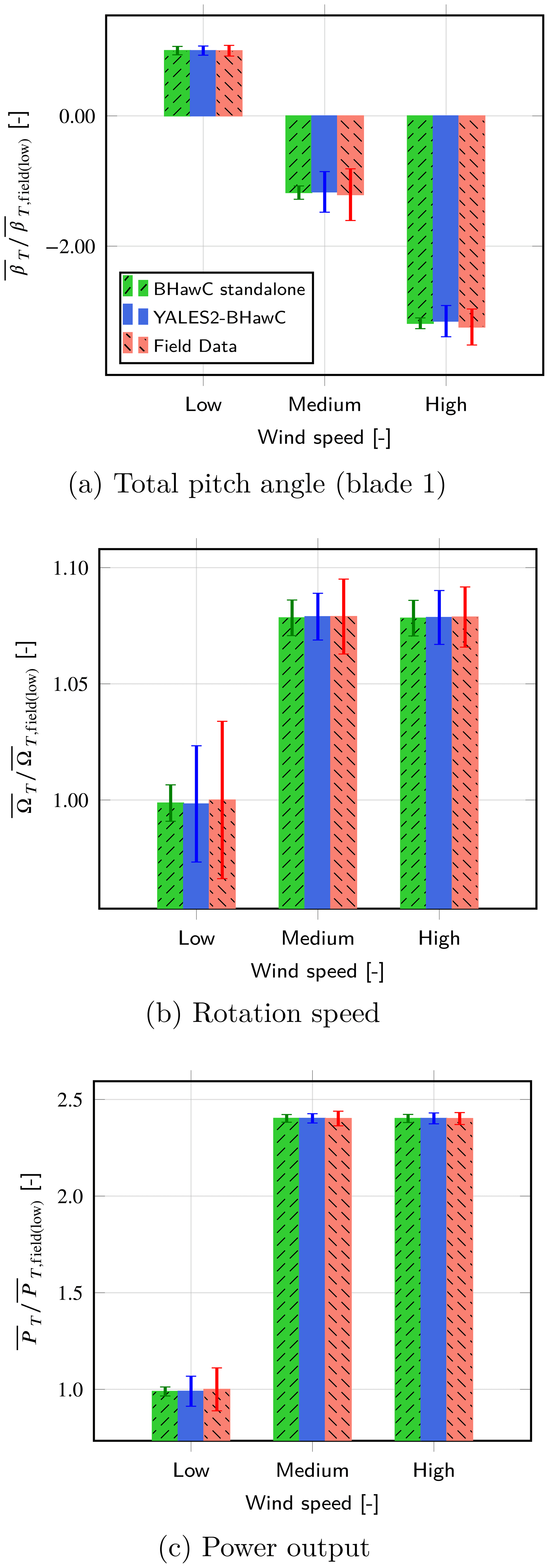
Figure 9Comparison of the time-averaged rotation speed, total pitch angle (first blade), and power, for the three wind speeds of interest. The corresponding standard deviations are depicted as error bars.
The edgewise and flapwise bending moments at a spanwise position close to the blade root are compared for the first blade in Fig. 10. Field data were also available for such quantities thanks to strain gauges. Again, the results numerically obtained with both codes are fairly accurate. Discrepancies, reaching up to 20 % of the field data, are visible, but the trends are very well captured.
Figure 10Comparison of the time-averaged edgewise and flapwise bending moments, on the first blade and at the strain gauge location. The standard deviations are depicted as error bars.
In what follows, the numerical results are now compared in greater detail. Despite the lack of field data for the quantities considered, the results from BHawC stand as a reference. Indeed this tool is a keystone in the design cycles of actual turbines and thus has been extensively validated against field data in those specific conditions (no yaw error and no upstream wake).
The first-blade tip deflection δf in the flapwise direction YBB BH is compared for all wind speeds in Fig. 11. Results of both codes are depicted for N=10 rotor full revolutions. The periodicity due to the rotor revolution is clearly visible in the two signals, while the turbulent inflow causes additional fluctuations. One can note significant differences between the curves. This is expected as the rotor azimuth at a given time has no reason to be the same in the two simulations. Indeed, inductions at the aerodynamic nodes' location are not computed in the same way, which leads to different aerodynamic loads and in the end to a different feedback from the controller. Besides, the turbulence seen by the rotor is not exactly the same in both codes, even initially. The reason is further developed later in this section. Yet, the amplitude of the deflections compares very well for all wind speeds.
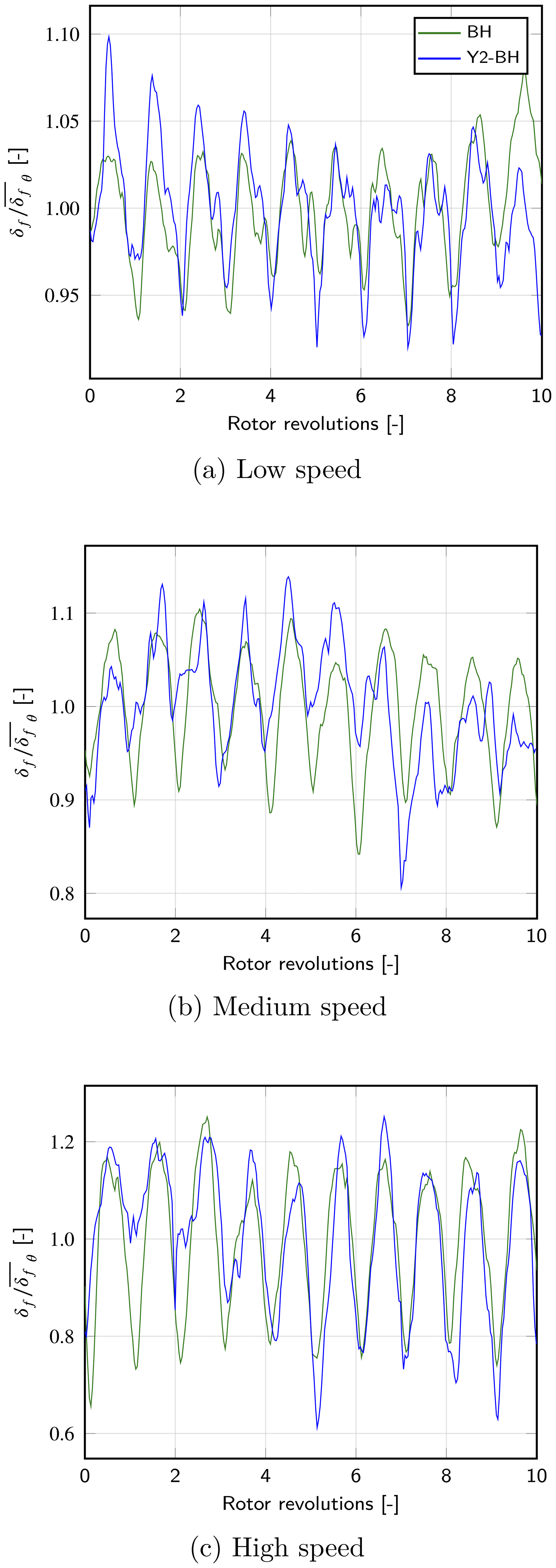
Figure 11Comparison of the first-blade tip deflection δf, in the flapwise direction, over the 10 last revolutions of the rotor, as obtained by BHawC and YALES2–BHawC.
In Fig. 12, the comparison is continued in polar coordinates to visualize the distribution of discrepancies according to the azimuthal position. To this end, we compare the mean deflection obtained at 36 azimuthal positions, based on the data from the last N=50 revolutions of the rotor. Overall, the results from both codes agree fairly well at all wind speeds, with discrepancies mostly lying in the range . No clear trend appears, meaning the coupled code does not tend to either over-predict or under-predict the results from BHawC. The local gap between the results peaks in the azimuthal range , for the high-wind-speed case, where the deflection predicted by YALES2–BHawC is on average 10 % higher than the one computed by BHawC. For the medium wind speed, we can notice that the discrepancies also reach their maximum (in algebraic values) in the same azimuthal range. However, the same cannot be said for the low-wind-speed case, where the relative difference in the results remains constant over all the azimuth positions. This behavior is not fully understood yet. It may be related to the turbulence injected in YALES2 not being in equilibrium with the mean flow, especially close to the ground. An artificial boundary layer developing on the bottom wall from the inlet was indeed observed. Its thickness increased while moving downstream, all the more at low wind speed to encompass the whole rotor. In the high-wind-speed case, on the other hand, this artificial boundary layer only partially overlaps the rotor area.
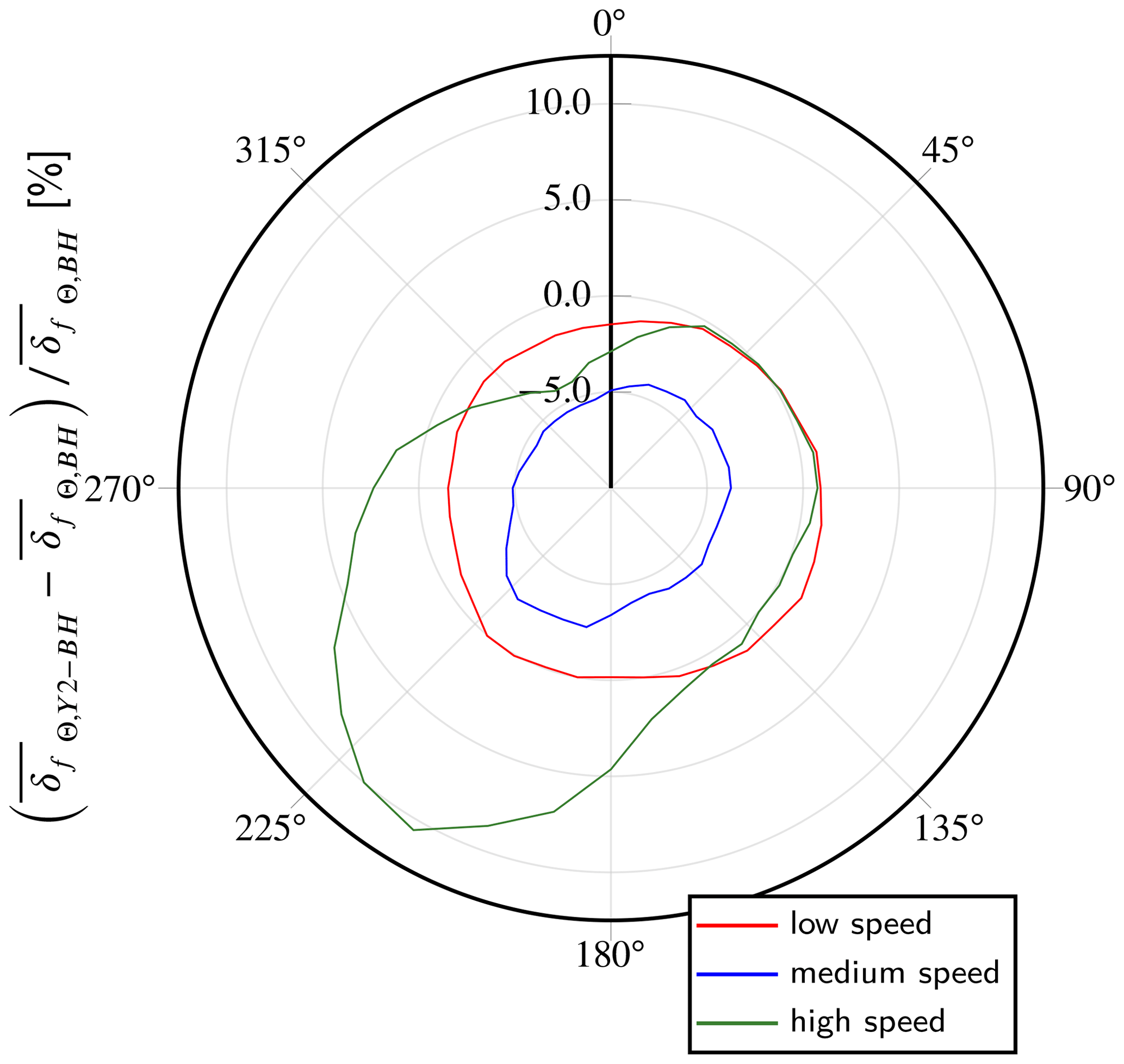
Figure 12Comparison of the first-blade tip deflection δf in the flapwise direction, averaged per azimuthal position. The data from the last 50 revolutions of the rotor are considered.
To deepen the analysis, Fig. 13 compares the frequency decomposition of the flapwise deflection just discussed for all the investigated wind speeds. To get representative results, the data from the last N=50 revolutions of the rotor were considered input. For each wind speed, the main peak matches the frequency frot, derived from the time-averaged rotation speed of the rotor. This peak, as well as its two first harmonics, is well captured by both codes. In the three wind speed scenarios, a good overlap between the results from BHawC and YALES2–BHawC is obtained overall. Nonetheless, the peaks are slightly more diffused in the results of the coupled code. This is consistent with the standard deviations of the rotation speed being higher in YALES2–BHawC than in BHawC (see Fig. 9).
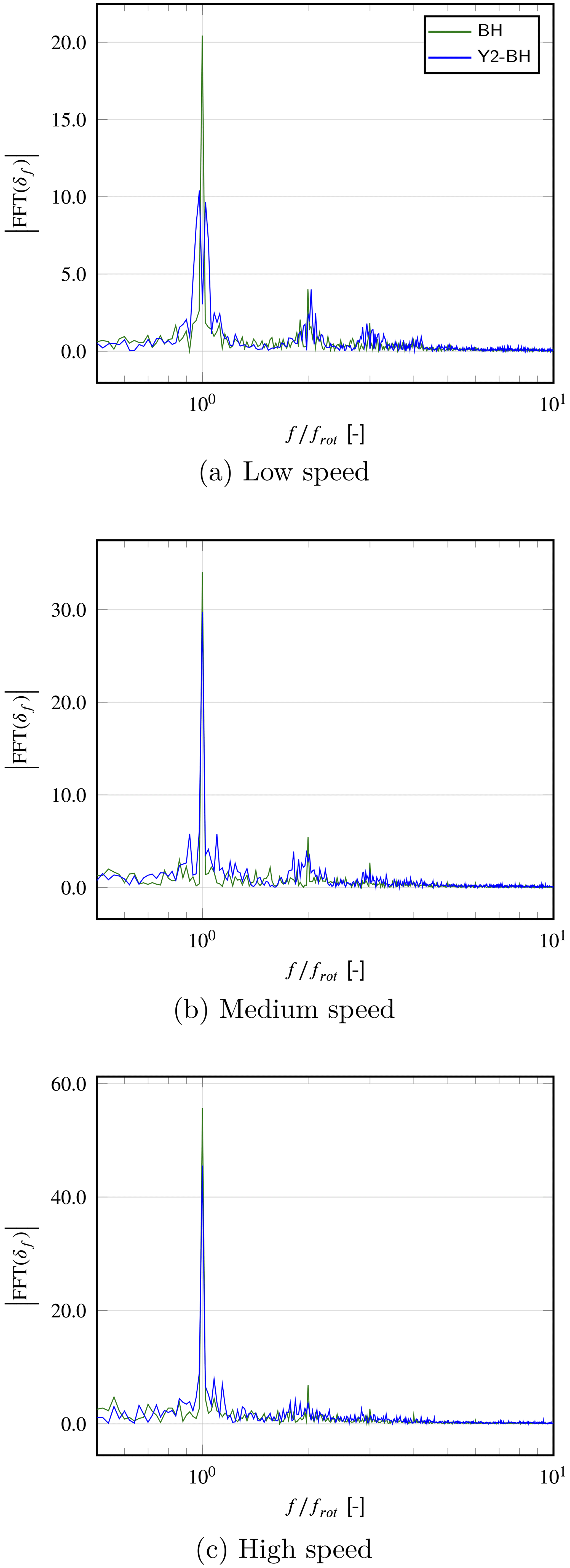
Figure 13Fast Fourier transform of the first-blade tip deflection δf in the flapwise direction, considering the results from the last 50 revolutions of the rotor for both YALES2–BHawC and BHawC.
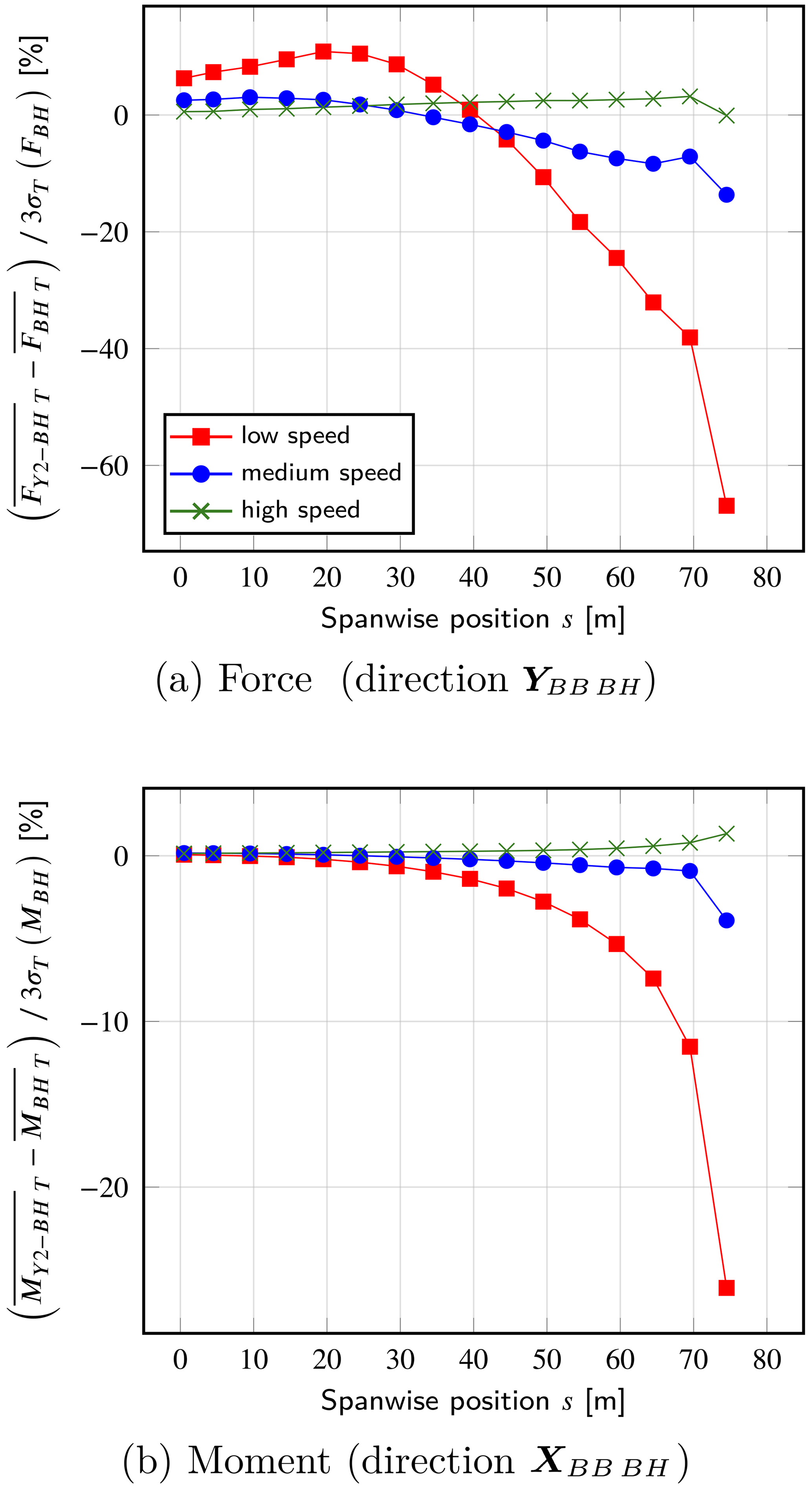
Figure 14Comparison of the internal loads (forces and moments) at several spanwise positions across the first blade. The quantity σT(•) refers to the standard deviation of the argument over the time range T.
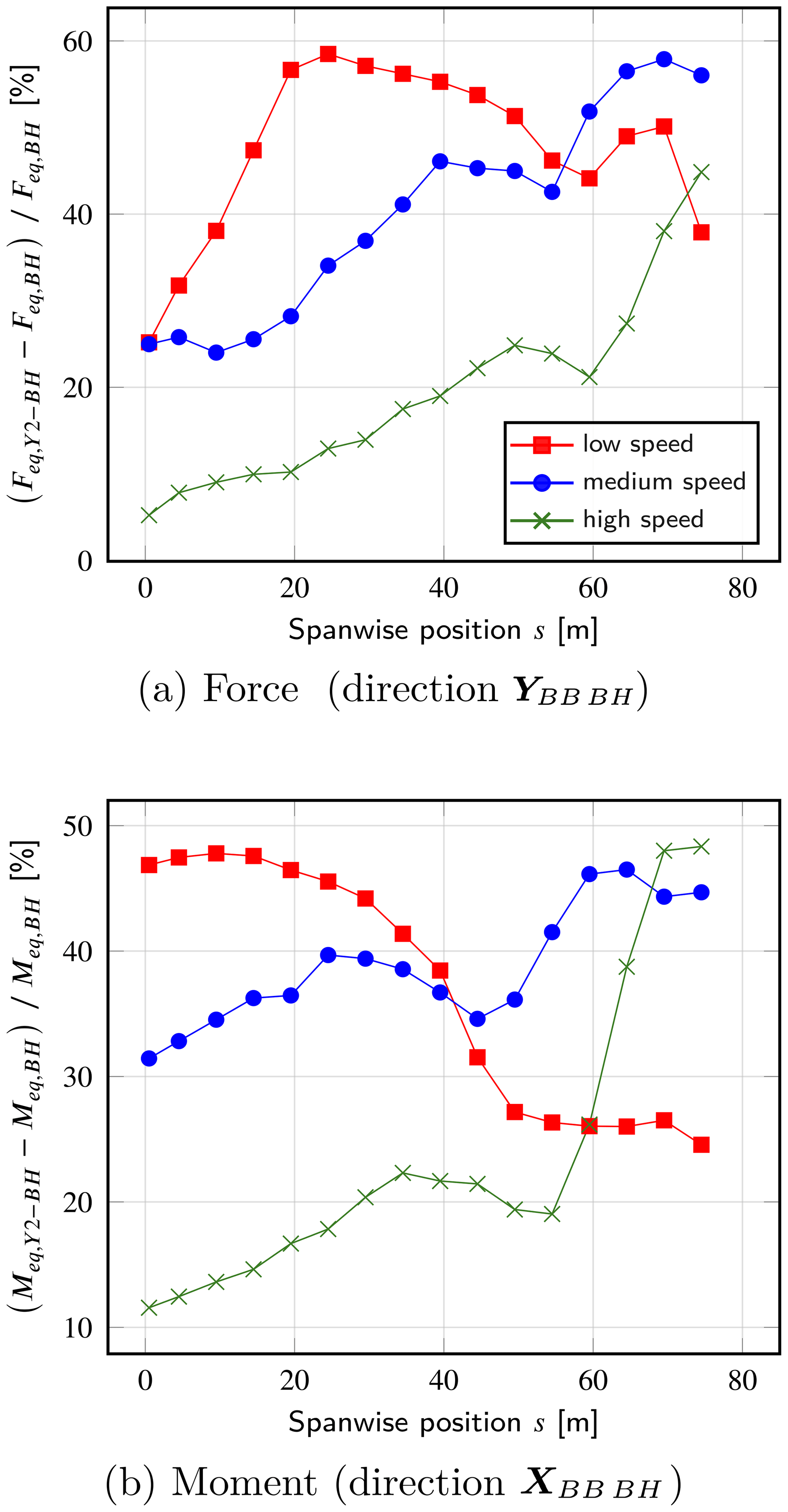
Figure 15Comparison of the damage equivalents loads, computed from the internal loads (forces and moments) at several spanwise positions across the first blade.
The time-averaged internal force F and moment M obtained in the flapwise direction YBB BH and edgewise direction XBB BH, respectively, are now compared at several spanwise positions across the first blade. The results are provided in Fig. 14 for all the wind speeds of interest. The discrepancies between the results from YALES2–BHawC and BHawC are given relatively to 3 times the standard deviation in time σT of BHawC results. Most of the discrepancies appear to lie within the range [−10 %, 10 %]. Still, one can observe higher gaps in the low-wind-speed case, especially close to the blade tip, where the loads computed by YALES2–BHawC are shown to be significantly lower than those coming from BHawC standalone. Nevertheless, it seems important to stress that the standard deviations in time of the depicted loads, as their time-averaged values, become smaller and smaller when heading towards the blade tip, to be almost zero at the tip.
The variability in the internal loads in time is also of great interest for engineers as it conditions the structural fatigue. Thus, the damage equivalent loads (DELs) were computed from the internal loads F and M just discussed. The Palmgren–Miner rule (Miner, 1945) allows the assessment of the damage d of a blade element, resulting from an unsteady internal force F (or moment M) acting during the period T:
The whole variation range of F is split into Nb bins, which define as many discrete amplitudes Fj for the included loading cycles. A rainflow algorithm (Matsuishi and Endo, 1968) is used to count the number of cycles nj associated with each amplitude Fj. The quantity denotes the maximum number of loading cycles of amplitude Fj that the blade element can withstand before breaking by fatigue. Simply put, the previous law states that a pure sinusoidal load F′, of amplitude Feq and frequency , will lead to the same damage as the real load F would. The number of cycles is usually provided through a Wöhler curve (also known as S–N curve), which can be fitted by the following law:
where k and m are material-dependent properties. For a wind turbine blade, even though it may vary with the deformation direction, the value m=10 is traditionally used (Sutherland, 1999; Lee et al., 2012), as it refers to the glass fiber which comes in the composition of the blade reinforced parts (Mishnaevsky et al., 2017). The combination of Eqs. (20) and (21) leads to the following expression for Feq:
Only the choice of the frequency feq remains. In order to compare the results from all cases, we set feq=1 Hz, which is decorrelated from the wind conditions.
The relative differences in the results obtained are reported in Fig. 15. They are shown to be significantly higher than those observed in the results commented on previously. This is particularly true for the low-wind-speed and medium-wind-speed cases, for which the equivalent loads predicted by YALES2 exceed those of BHawC by about 30 % on average, considering the entire blade span. Two trends are also noticeable depending on the wind speed. In the medium-wind-speed and high-wind-speed cases, the discrepancies increase from the root to the mid-span region and then tend to decrease slightly before significantly increasing back when heading towards the blade tip. On the contrary, the discrepancies obtained in the low-wind-speed case evolve differently, especially for the flapwise equivalent moment, for which they are maximum in the blade root region.
4.3 Discussion on the reported discrepancies
Given their amplitude, the gaps observed in the numerical results reported in the previous sub-section likely relate to three main factors. First, as mentioned at the end of Sect. 3, BHawC includes the model of Beddoes–Leishman (Leishman and Beddoes, 1989) to take into account the dynamic stall effect and correct the aerodynamic coefficients accordingly. As suggested by Øye (1991), the dynamic stall effect can be roughly translated into a time relaxation of the aerodynamic loads. Disabling this model in BHawC was impossible in practice, as this led to the failure of the structural solver.
Second, BHawC computes annular inductions, which could also weaken the shear-induced variability in the aerodynamic loads inferred afterwards.
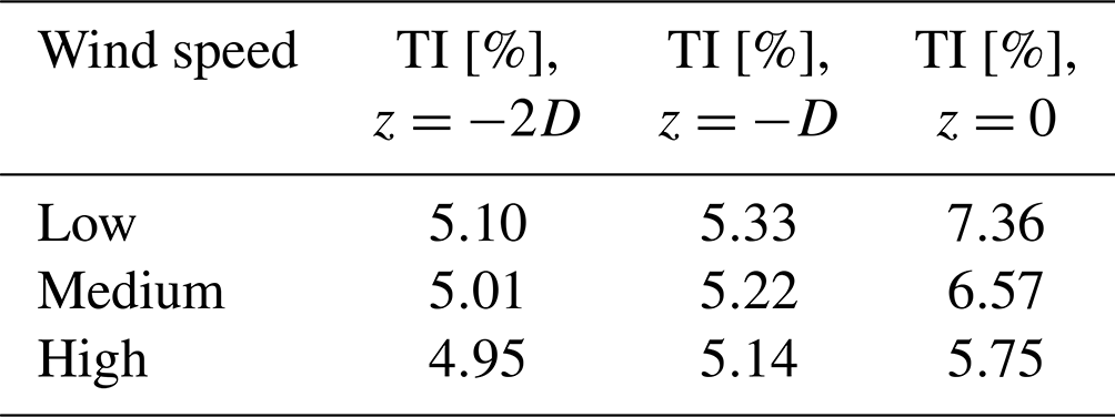
Third, the turbine in BHawC does not exactly face the same turbulent structures as in the coupled code, primarily because the relative position between the turbine and the turbulence box differs. Besides, the turbulence is static in BHawC, meaning the velocity fluctuations factored into the induction computation are the ones present in the Mann boxes. Similarly, the shear profile remains equal to the one provided at all times. On the other hand in YALES2–BHawC, the Mann turbulence will evolve while being convected to the rotor position, especially close to the ground. A slight distortion of the shear profile is also expected. Such shortcomings directly result from the unbalanced combination of the injected synthetic turbulence, the power law, and the boundary conditions (especially the one used at the bottom boundary). To better illustrate this, the streamwise time-averaged velocity and the streamwise turbulence intensity considered in both YALES2–BHawC and BHawC are depicted in Figs. 16 and 17. It can be seen that the turbulence injected at the inlet in YALES2 first tends to decay at hub height, while it significantly increases close to the bottom boundary and then induces the most significant distortions of the shear profile. As complementary results, the mean turbulence intensity in the projected rotor area was assessed in all coupled simulations at several streamwise positions: one and two diameter(s) upstream of the turbine as well as in the rotor plane. The obtained values are gathered in Table 2. Considering the low-wind-speed and medium-wind-speed cases in the rotor plane, it appears that the turbulence intensity is above the target values from Table 1. While this overall issue cannot be fully worked around, one way to address it would be to replace the Mann boxes in BHawC with velocity fluctuations extracted from the YALES2–BHawC simulation, say one diameter upstream of the turbine (Houtin-Mongrolle, 2022).
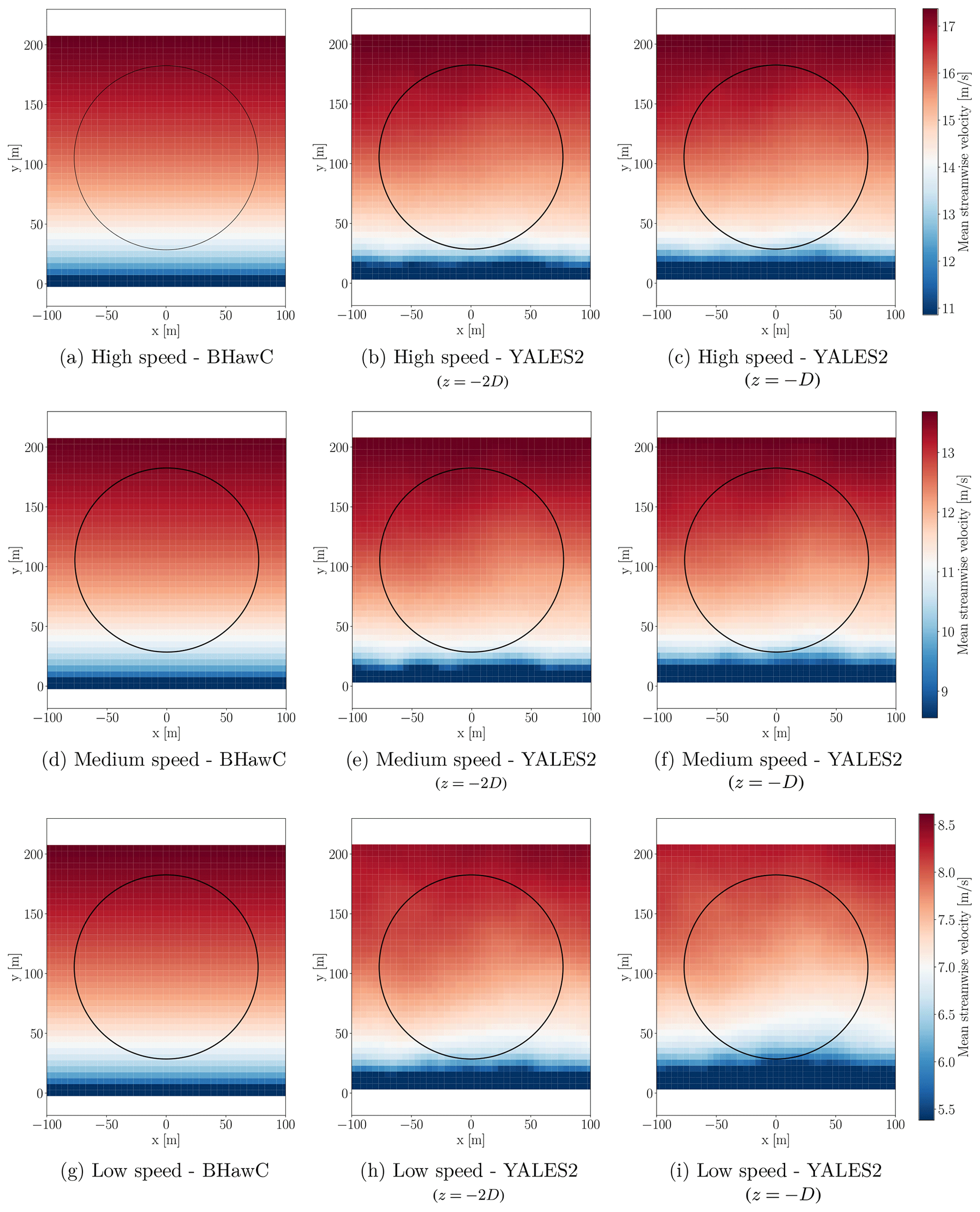
Figure 16Comparison of the shear profile imposed in BHawC (left column) with the one actually obtained in YALES2–BHawC two diameters and one diameter upstream of the rotor. The rotor position is depicted in each plot as a black circle.
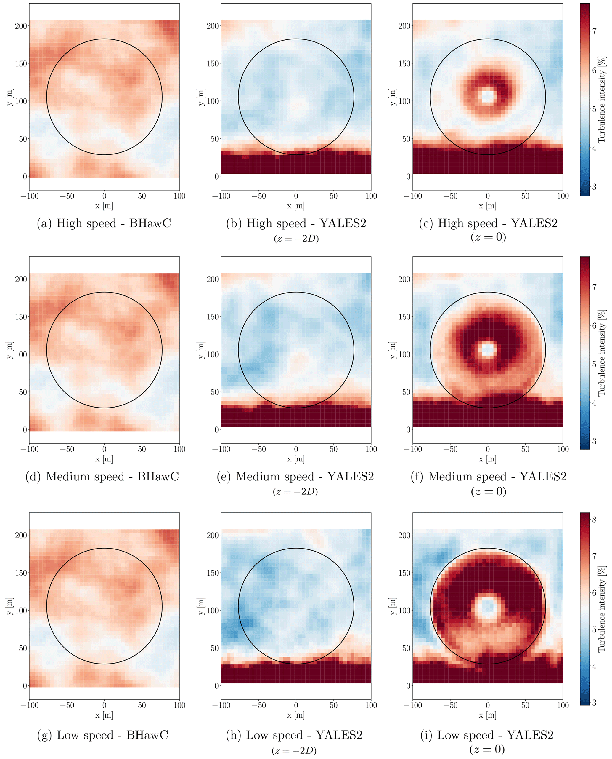
Figure 17Comparison of the turbulence intensity imposed in BHawC (left column) with the one actually obtained in YALES2–BHawC two diameters upstream of the rotor and in the rotor plane. The rotor position is depicted in each plot as a black circle.
Table 2Mean effective streamwise turbulence intensities obtained in YALES2–BHawC one and two diameters upstream of the rotor, as well as in the rotor plane, in the projected rotor area.
Considering all the aforementioned sources of discrepancies, the results given by the code YALES2–BHawC for the structural part are therefore deemed encouraging and promising. As for the prediction of the main operating parameters and performance of the turbine, the coupled code already provides accurate results. Even though additional investigations are definitely needed, the results so far presented constitute an encouraging first step towards a full validation of YALES2–BHawC.
4.4 Surrounding flow
Unlike BHawC standalone, YALES2–BHawC provides insights into the flow surrounding the turbine. For all the wind speeds considered, Fig. 18 presents the streamwise instantaneous velocity field and the corresponding time-averaged field in vertical slices. All the fields shown are divided by the related target velocity at hub height Uh to allow easy comparisons. One can observe the wake regions to be very different. The velocity deficit behind the turbine is indeed stronger in the low-wind-speed scenario, which is indicative of a significantly higher induction. This is consistent with the low wind speed being slightly below the rated one. Conversely, the velocity deficit obtained at high wind speed is about 20 %. This is caused by the rotation speed being only 8 % higher than in the low-wind-speed case (see Fig. 9) while the wind speed is close to being 100 % higher. Therefore the resulting blockage effect is lower. Additionally, the cell size mapping used in the mesh allows the representation of a wide range of velocity fluctuations, both upstream of the turbine and in the wake.
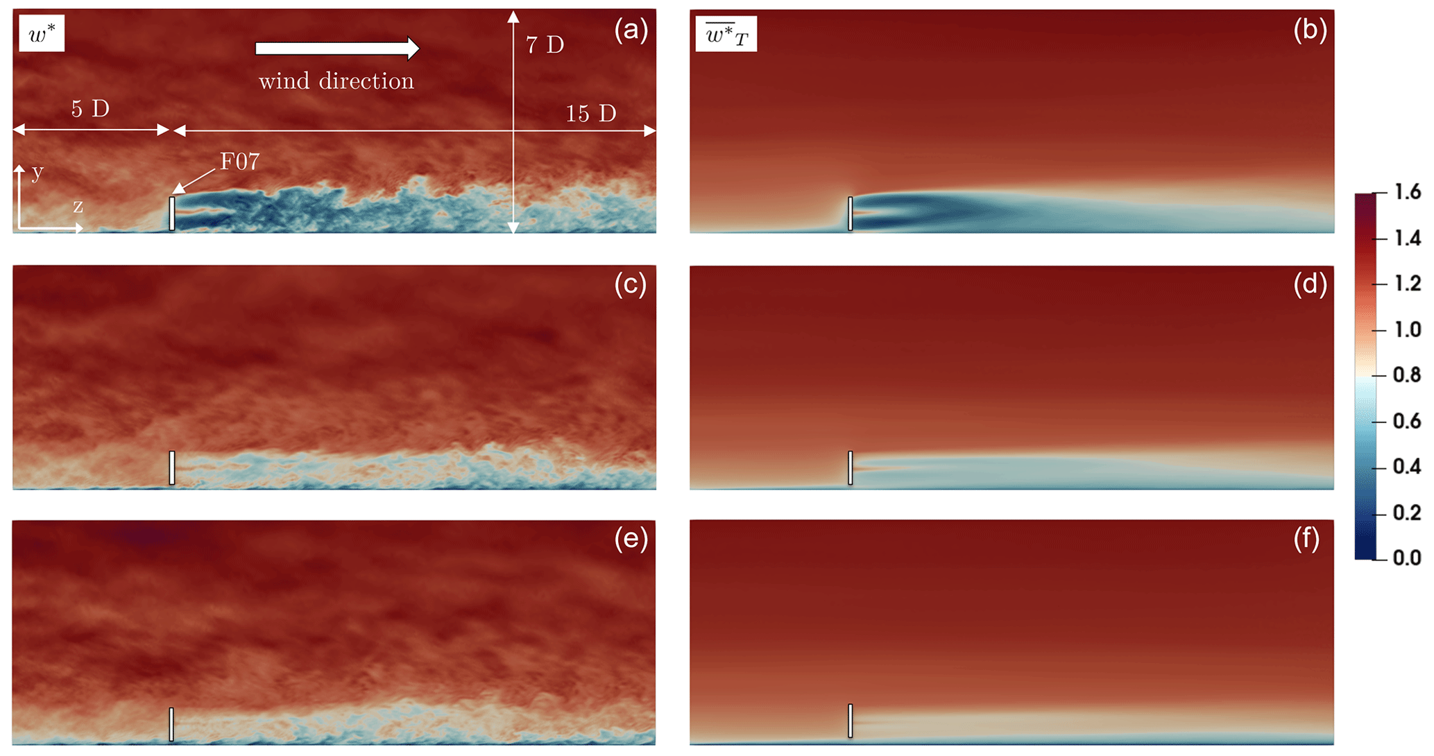
Figure 18Vertical slices, including the rotor center, of the instantaneous (a, c, e) and time-averaged (b, d, f) streamwise velocity fields for the low (a, b), medium (c, d), and high (e, f) wind speeds. Extents of the region focused on are given in a number of rotor diameters D.
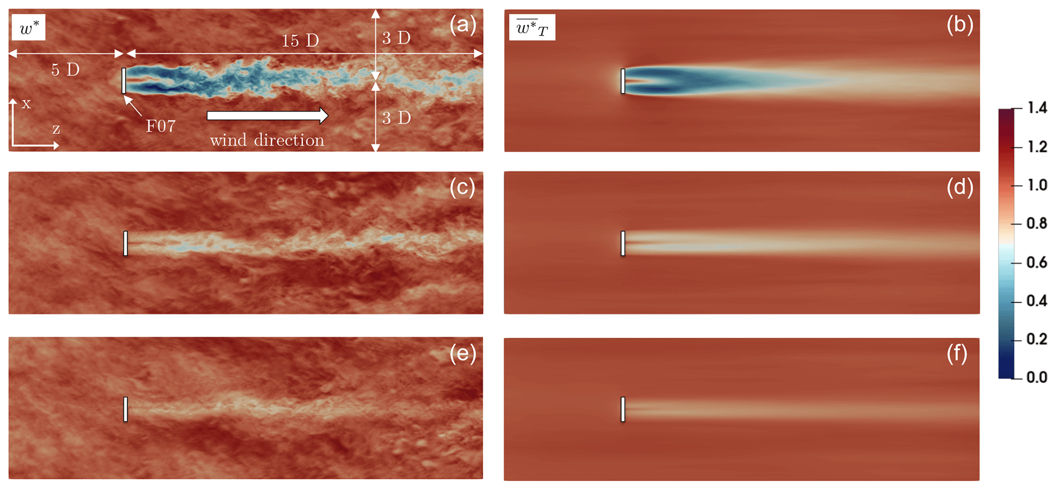
Figure 19Horizontal slices, taken at hub height, of the instantaneous (a, c, e) and time-averaged (b, d, f) streamwise velocity fields for the low (a, b), medium (c, d), and high (e, f) wind speeds. Extents of the region focused on are given in a number of rotor diameters D.
Figure 19 shows the same fields but in a horizontal plane taken at hub height. The comments made previously stand, but one can further notice some meandering in the wake, especially at low wind speed.
4.5 Computing performance
Finally, we briefly report the computing performance obtained with BHawC standalone and YALES2–BHawC. All the numerical simulations previously commented on were run on the AMD Rome partition of the Joliot-Curie supercomputer from TGCC. The simulations carried out with BHawC standalone (BH) were handled with only one CPU core, as the code is fully serial, while all the coupled simulations (YALES2–BHawC: Y2-BH) used 255 CPU cores: one for BHawC and the remaining ones for YALES2. The return time of each simulation, given per second of computed physical time, is reported in Table 3. In all cases, the exclusivity flag of the job scheduler was deliberately activated to achieve a better computing performance. Still, one should note that all the simulations were run only once to save CPU hours. Thus, the values given in Table 3 could be slightly biased. Yet, as expected, the return times of the coupled simulations are shown to be significantly higher.
Table 3Return times of the numerical simulations, given per second of computed physical time.
This paper first presents the details of a new aero-servo-elastic solver, obtained from the coupling between a high-fidelity massively parallel LES solver (YALES2) and an aero-servo-elastic solver (BHawC) in use in the wind energy industry. In this coupling, YALES2 completely replaces the BEM method normally used in the standalone version of BHawC, meaning that the aerodynamic loads come entirely from YALES2. Thus designed, the coupled solver allows one to obtain a detailed picture of the flow surrounding an actual wind turbine (or even a wind farm), where the effects of the flexible rotating blades are factored in thanks to an elastic ALM framework. Besides, the coupled solver also enables the investigation of the structural response of each individual blade, within the limits set by a 1D beam modeling approach. Profiting from an emulation of real control strategies, the variation over time of the main operating parameters (rotor rotation speed and pitch angles) can be considered to predict a turbine power output realistically.
For validation sake, we considered the case of an isolated turbine of the Westermost Rough offshore wind farm. The power output obtained numerically, as well as the rotation speed and pitch angles, was compared to field data derived from 10 min on-site recordings. Overall, an excellent agreement was pointed out. Difficulties in translating the actual incident wind into boundary conditions may explain the remaining discrepancies. To deepen the validation process, the deflections and internal loads of the blades, predicted by both YALES2–BHawC and BHawC, were compared. Again, the results agreed reasonably well, despite the discussed differences in the numerical setups and in how the local inductions are computed. Further investigations will be needed to assess the exact causes of the observed discrepancies. Nevertheless, the reported results can be seen as a first encouraging step towards a full validation of YALES2–BHawC.
As a final word, it seems important to stress that, from an industrial perspective, the coupled code YALES2–BHawC remains too demanding in memory and CPU resources and too time-consuming to be used directly in actual design cycles. However, as field data do not always provide insights into the physics involved, this tool can be used advantageously to help in designing, calibrating, and certifying lower-order approaches such as the BEM method or wake engineering models. Because those are computationally affordable and predictive, they are indeed used on a daily basis in the industry to assist mechanical design and siting studies.
Before attempting real-application cases, the coupled code YALES2–BHawC has been extensively checked. Relying on appropriate unit tests, we verified both the kinematic and the dynamics aspects involved in the coupling.
Discussed in Sect. A1, the kinematic verification is carried out by comparing the results from simulations run with YALES2 standalone (Y2) and YALES2–BHawC (Y2-BH), respectively. On the other hand, the verification of the dynamic aspects, reported in Sect. A2, is supported by a comparison of the results obtained with BHawC standalone (BH) and YALES2–BHawC. In all cases, we consider the SWT-6.0-154 wind turbine model (Siemens Gamesa Renewable Energy, 2014), whose rotor diameter D is 154 m.
The rotor rotation speed is fixed to a constant value in YALES2 standalone, as it is the most straightforward approach. However, this cannot be enforced as easily in BHawC and in the coupled code. Indeed, BHawC needs a controller component to adjust the rotation speed. A simulation can still be run without it, but the rotation speed will then increase progressively without any limitation. Given the structural modifications of the blades that were also necessary to complete the verification activities, targeting a given rotation speed in BHawC with the actual controller was considered too challenging. We thus replaced this controller by a dummy one, designed to track a user-supplied rotation speed by adjusting the rotor torque only.
In both YALES2 and BHawC, the incident flow is chosen to be uniform with no synthetic turbulence added, and its speed is set to 8 m s−1. Besides, for the sake of similarity, we nullified the induction factors in all simulations. In YALES2, the resulting flow is thus uniform throughout the whole domain, which allows the use of a narrow computational domain (as illustrated in Fig. A1), along with a very coarse Cartesian grid (cell size ∼12.5 m).
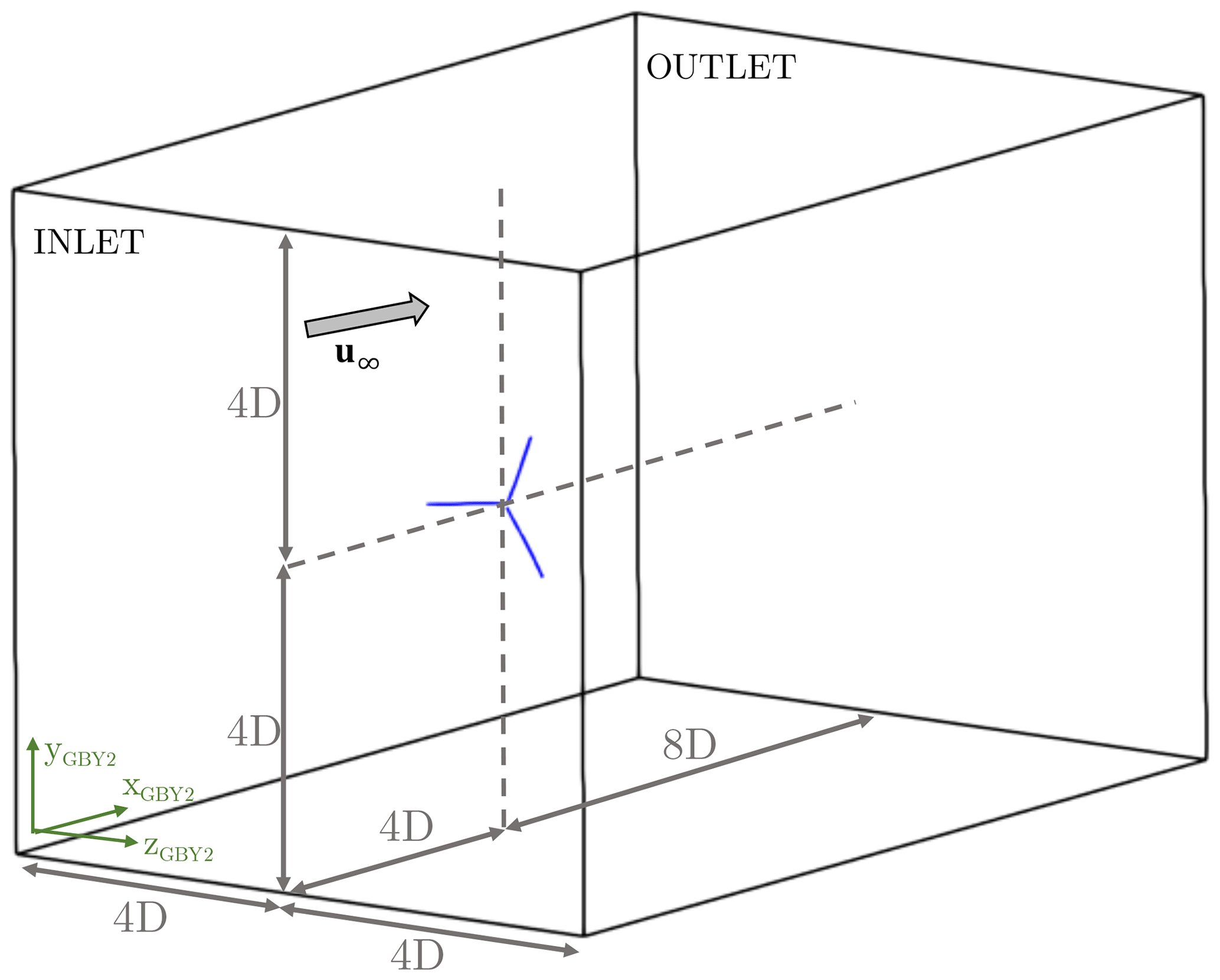
Figure A1Geometry of the computational domain used with YALES2 and YALES2–BHawC during the verification campaign.
In all numerical setups, the blades are equally discretized: 75 aerodynamic nodes/particles are evenly distributed along the blades' span. The lookup table used in YALES2 was built to contain the blade data that BHawC would attach to its aerodynamic nodes in such a configuration. This way, blade data at the particles' location in YALES2 are forced to match those used in BHawC, as interpolation errors are avoided.
Besides, the blades' elasticity and shear moduli are chosen to be 1000 times larger than the actual ones, almost nullifying the blade deflections. Obviously, this does not apply to YALES2 standalone simulations where blades are fully rigid. Consistently, the remaining wind turbine sub-structures present in the structural solver are also modeled as almost fully rigid, and the aerodynamic loads acting on them are nullified.
A1 Kinematic aspects
As explained in Sect. 3, in a coupled simulation BHawC communicates to YALES2 the position and velocity of all actuator line (AL) particles, as well as the 3D basis attached to them. Therefore, we need to ensure, at first, that the AL particles in YALES2–BHawC are moving as they would in YALES2 standalone. The results obtained with both codes using the configuration previously described are thus compared. However, two differences between the numerical setups must be stressed, as they cannot be removed. The first one concerns the blades: they are fully rigid in YALES2, while they almost are in YALES2–BHawC. As a result, the blades in the coupled simulation necessarily experience tiny deflections. The second difference is related to the rotor rotation speed: it is imposed as constant throughout the whole simulation in YALES2, while a transient state occurred in the coupled code because of the dummy controller. For this reason, we waited for the rotation speed to converge in YALES2–BHawC before considering the results. In the following, we display the mean error and corresponding standard deviations obtained between the two codes for various quantities of interest. A mean error is defined as follows:
where • is one of the quantities of interest and θN is the total azimuth angle swept by the blade during the N last full revolutions of the rotor. For this verification study, N was set to 10.
First, the effect of the residual blade deflection on the particle position should be quantified. Figure A2 shows the average difference in the particles' x, y, and z coordinates in the blade basis nondimensionalized by the blade length Lblade=75 m. The maximum deformation occurs at the tip of the blade and is oriented in the flapwise direction YBB BH, which is also the streamwise direction. As expected, this deformation is still very small compared to the length of the blade. The spanwise stretching (direction ZBB BH) and edgewise bending (direction XBB BH) are about 10 times smaller and thus neglected in the following analysis. Standard deviations are also given in the figure but are barely (if not) visible as they are extremely small.
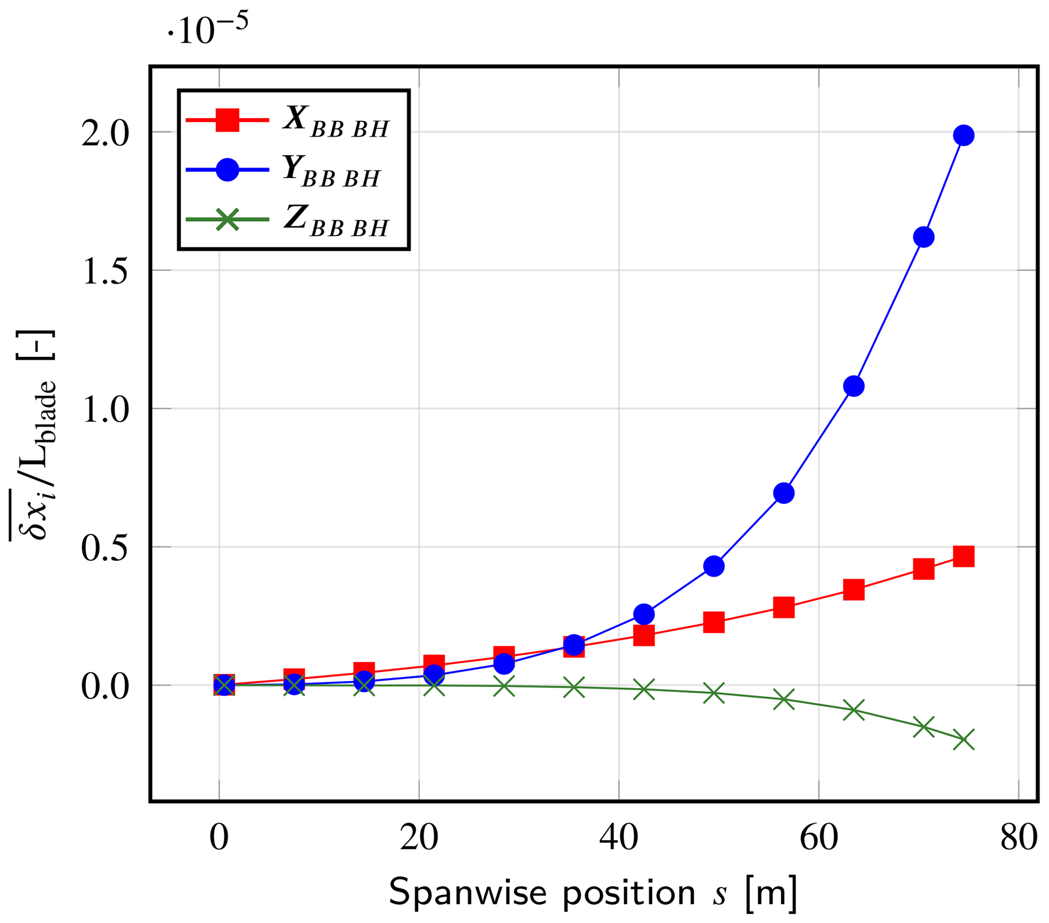
Figure A2Nondimensional mean discrepancy between YALES2 and YALES2–BHawC at the particle position xP in the BHawC blade basis, given as a function of the spanwise position. Residual blade deflection due to the structural flexibility of the YALES2–BHawC solver is small compared to the blade length. The corresponding standard deviations are represented as error bars (not visible).
Similarly, the orientation of the particle bases is also checked. To perform the comparison, we compute the dot product between the respective particle-basis x, y, z vectors of the YALES2 standalone and coupled simulations. As depicted in Fig. A3, the dot products are all very close to 1, which means that the particle bases are equally oriented. The standard deviations are also provided here but again are too small to display. These first results lead us to conclude that the particle position and related bases are correctly retrieved from the data sent by BHawC in a coupled simulation.
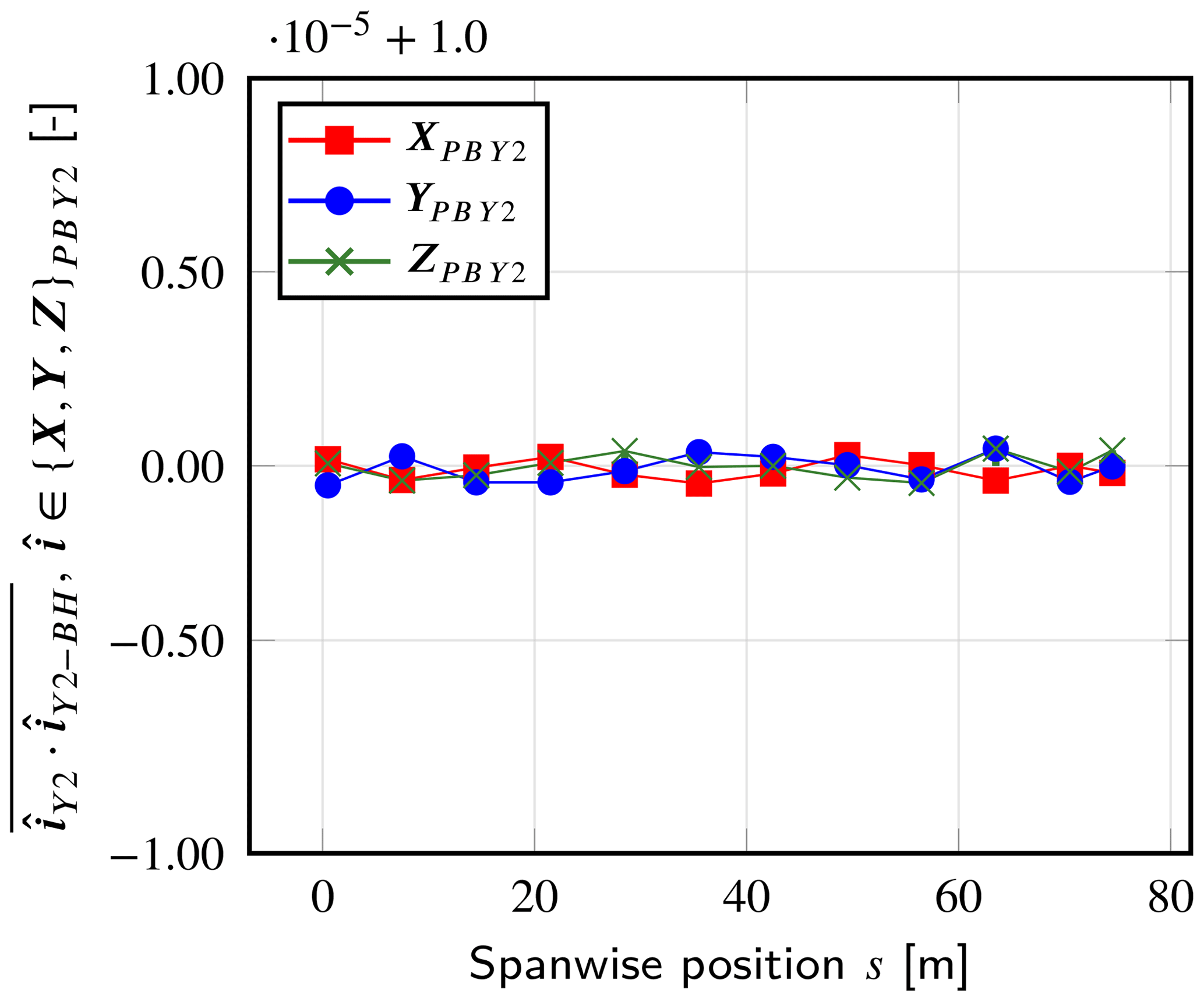
Figure A3Mean dot products between the particle bases obtained in YALES2 and YALES2–BHawC. Results are given as a function of the spanwise position. The associated standard deviations are represented as error bars (not visible).
The next step is to check the particle velocity, which is also part of the communications between BHawC and YALES2 (see Eq. 12). Figure A4 shows the errors for the three velocity components, expressed in the global basis of YALES2. A particle velocity in the streamwise direction (direction XGB Y2) is due to the tilt angle and to the potential flapwise deflection of the blades. The discrepancies observed on this velocity component are about 10 times smaller than those for the other two components that mainly evolve in the rotor plane. For these two, the error grows linearly with the blade span to be maximum at the tip. This is easily related to the remaining flexibility of the blade in YALES2–BHawC. Overall, the mean errors and standard deviations remain small compared to the modulus of the rotational speed at the tip utip≈75 m s−1.
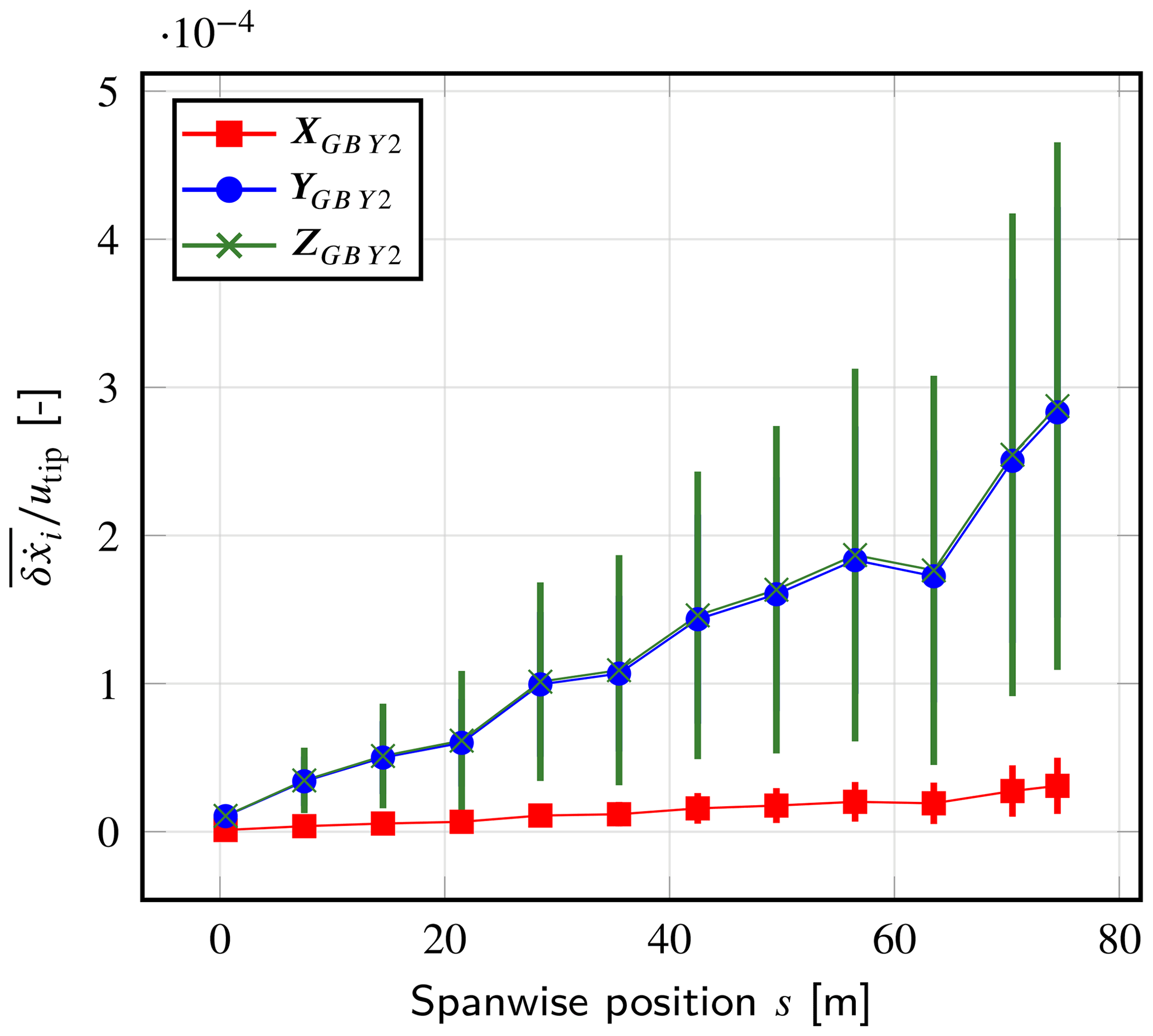
Figure A4Nondimensional mean errors in the particles' velocity , given in the YALES2 global basis. Results are given as a function of the spanwise position. The corresponding standard deviations are represented as error bars.
Finally, the angle of attack computed at each particle location is also looked at, as it contributes to the aerodynamic loads' computation. The discrepancies obtained between the two approaches are presented in Fig. A5. It can be observed that they remained below 0.012∘ on the whole blade span, which is completely acceptable.
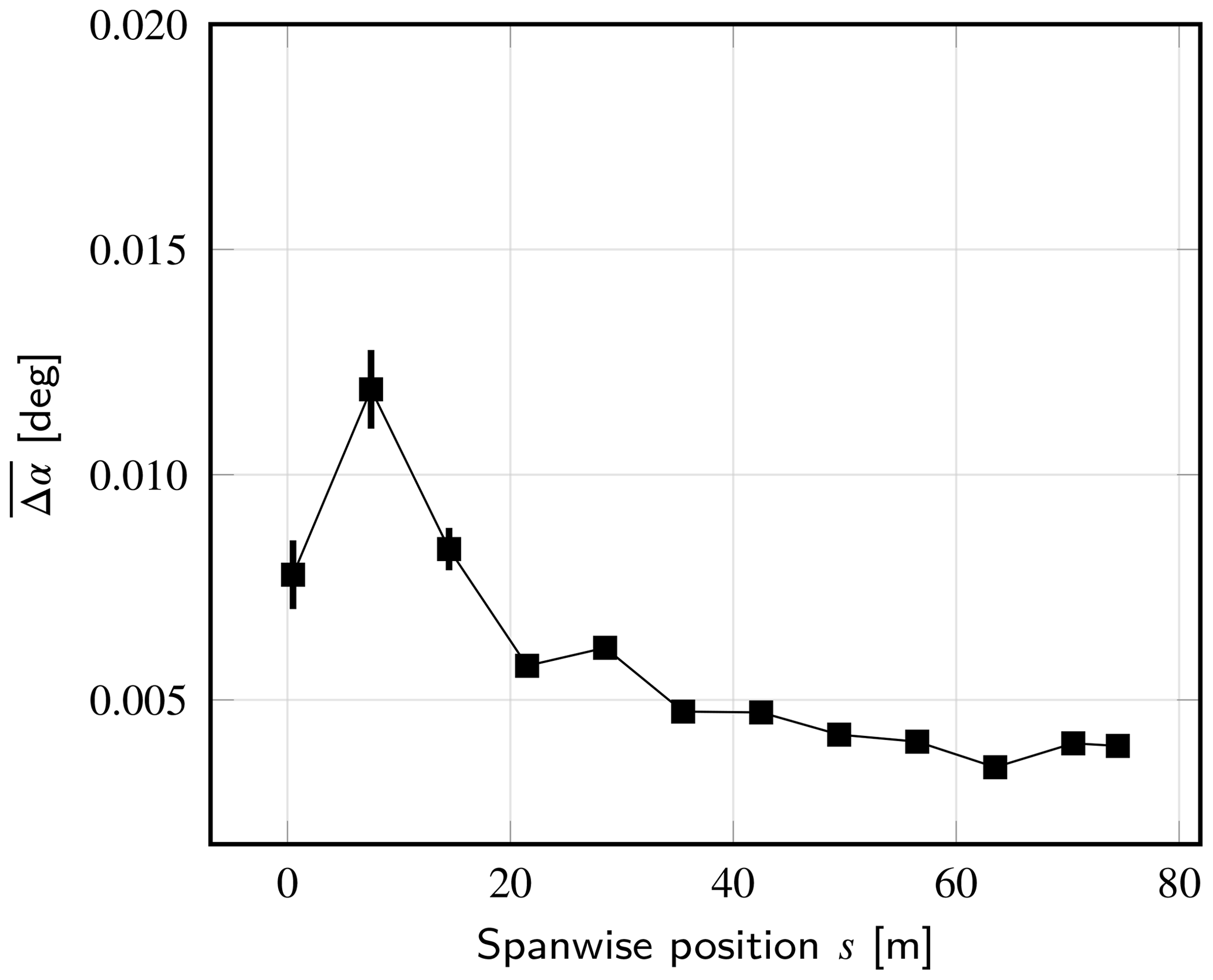
Figure A5Mean error in the angle of attack α, as a function of the spanwise position. The corresponding standard deviations are represented as error bars.
A2 Dynamic aspects
In order to consider the coupling implementation bug-free, an extra analysis of the aerodynamic loads is required. Indeed, the dummy controller used with YALES2–BHawC could make the rotation speed reach its target even though the predicted aerodynamic torque was completely wrong. Likewise, rigid blades cannot reflect a possibly poorly predicted thrust since their flapwise deflection would be close to zero.
To carry on this analysis, the internal loads computed by BHawC and YALES2–BHawC are compared. Indeed, with the induction removed in both cases, the BEM and AL methods should compute identical aerodynamic loads, as they are both downgraded to a simple polar reading. Consequently, the resulting internal loads computed by each code are also expected to be exactly the same. Here again, we use the configuration described at the beginning of the current section.
In both approaches, we consider the internal forces Fi and moments Mi (with ) in blade sections located at different spanwise positions s to build the following mean relative error:
where • stands for either Fi or Mi and θN is defined as in Sect. A1.
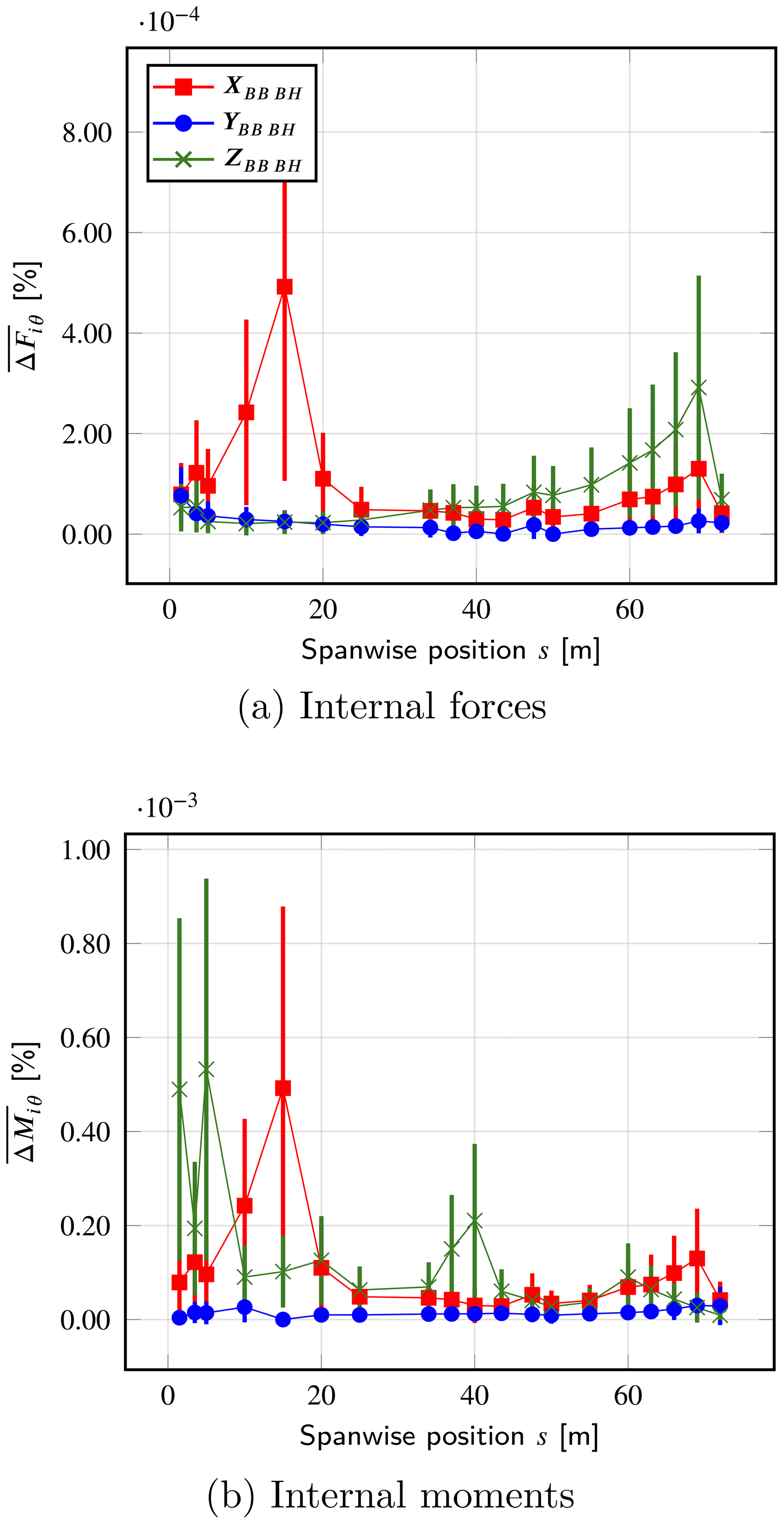
Figure A6Mean relative error in the internal loads, given as a function of the integration interval Δs. The corresponding standard deviations are depicted as error bars.
The results are given in Fig. A6. Overall the relative errors are very low, with values of less than 0.001%. The same observation applies to the corresponding standard deviations.
Explaining the remaining errors is not straightforward. In contrast to Sect. A1, the small deformations of the structure cannot be blamed as they exist in both simulations. However, the linear system solved by the structural solver proved to be ill-conditioned, likely because of the artificial stiffness added to the structure. Therefore, the structural responses could still significantly deviate even though the initial discrepancies in the aerodynamic loads were close to the machine single precision. Such differences are expected as BHawC and YALES2–BHawC rely on input files that are formatted differently. Nevertheless, the relative errors presented are deemed small enough to consider the coupled code fully operational.
No specific directive was included in the YALES2 library directly. Alternatively, an additional library is called dynamically from YALES2 to manage the communications with BHawC. This generic approach can be used to design a subsequent coupling between YALES2 and a BHawC-like code, such as OpenFAST (Jonkman and Buhl, 2005; National Renewable Energy Laboratory, 2022) or HAWC2 (Larsen and Hansen, 2007). Moreover, this new library was also coded in Fortran 90 to make all the subroutines of YALES2 readily accessible. However, this approach was not used with BHawC, which stands as an executable once compiled. For simplicity, communication directives were therefore written in BHawC directly. This architecture is outlined in Fig. B1.
All the required communications between the two codes were handled by means of the MPI library (Message Passing Interface Forum, 2021) (see Fig. B2). So defined, the coupling allows us to model both an isolated wind turbine and a wind farm. To each turbine corresponds a single BHawC process. Conversely, in YALES2, a turbine is known by all the MPI processes involved in the partition of the computational domain. This straightforward approach was chosen to easily comply with the mesh adaptation capabilities of YALES2, which may change the partition and cell groups initially known by a YALES2 process. Yet, this feature was not used in this work. An additional MPI communicator is created for each turbine, which encompasses the corresponding BHawC process and all YALES2 processes. In each communicator, the master rank is the BHawC process, which can thus be easily identified thereafter. All data exchanges between BHawC and YALES2 are carried out via these communicators. Data from BHawC are broadcasted to all YALES2 processes, while transfers from YALES2 to BHawC are achieved via point-to-point communications. At the beginning of the simulation, a YALES2 process is chosen to perform the latter. For convenience, this process is called the sub-master of the communicator. To balance the workload, a YALES2 process can be the sub-master of only one turbine communicator at most. The code will deviate from this scenario only when the turbines outnumber the YALES2 processes. Yet, this never happens during realistic simulations: the mesh size increases with the number of turbines, thus requiring the use of additional cores. Besides, each turbine is controlled independently of the others. No specific MPI communicator is therefore needed between the BHawC processes.
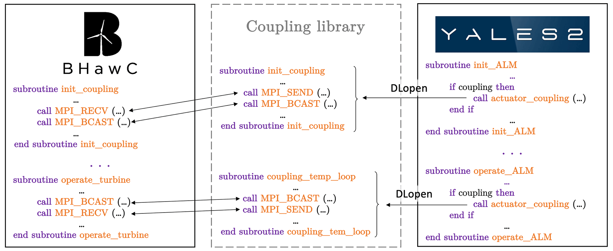
Figure B1Sketch of the coupling architecture. An external library is called dynamically from YALES2 to manage all the communications with BHawC.
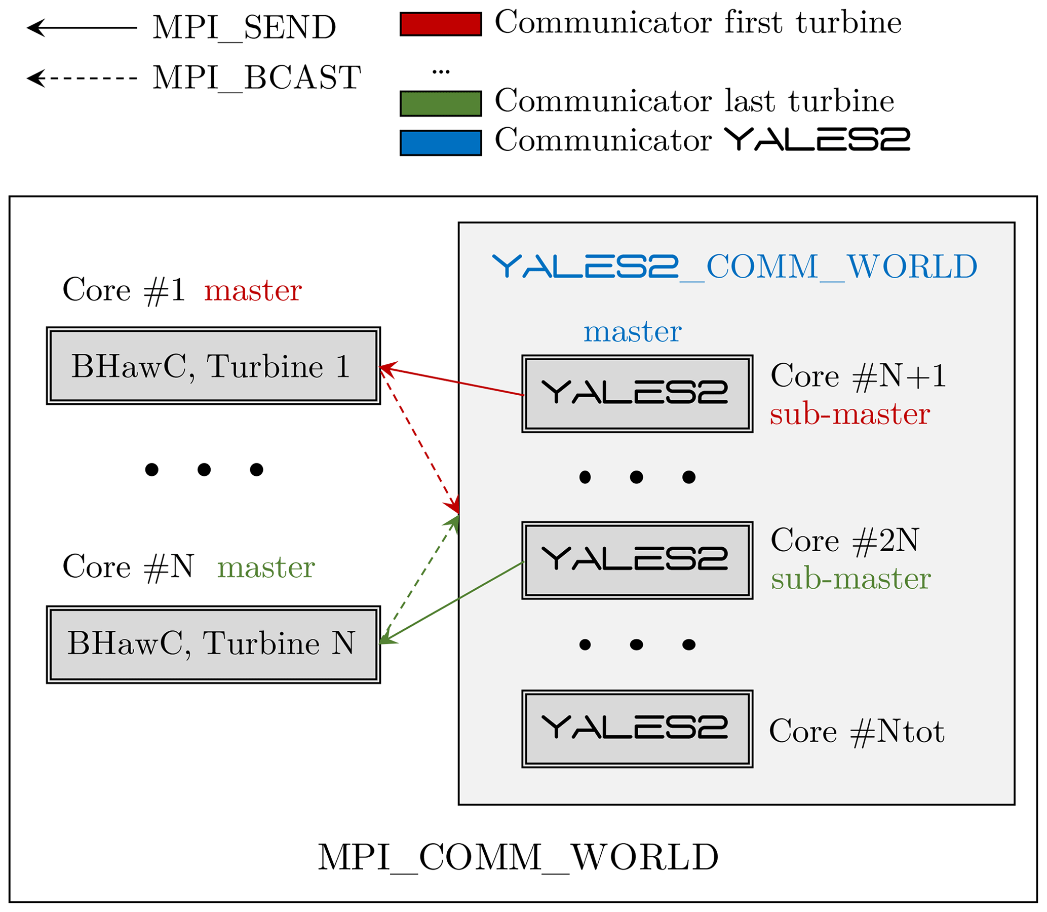
Figure B2Sketch of the MPI communications involved in the coupling between YALES2 and BHawC.
BHawC code (Rubak and Petersen, 2005) is proprietary software of the Siemens Gamesa Renewable Energy company, and its source code is strictly confidential. The YALES2 code (Moureau et al., 2011) is the property of CNRS (Centre National de la Recherche Scientifique); it is freely shared for academic studies and has a public website (https://www.coria-cfd.fr/index.php/YALES2, Moureau and Lartigue, 2023).
The raw field data used in this work have been generously provided by Ørsted to the authors but remain its private property. It is therefore not possible for the authors to disclose the initial data set. Similarly, all numerical results provided by YALES2 and BHawC cannot be shared for confidentiality reasons related to the simulated turbine design.
EM and SG both contributed to the following aspects of this work: conceptualization, methodology, software development, formal analysis, verification, validation, simulations setup and post-processing, and writing of the original draft and final paper. Valuable support was provided by FHM, BD, and PB regarding the conceptualization, methodology, and software development, as well as for reviewing the original draft. The field data were provided by BD. Finally, BD and PB were also in charge of the supervision, project administration, and funding acquisition.
Bastien Duboc declares that he was a full-time employee of Siemens Gamesa Renewable Energy at the time this work was carried out.
Publisher’s note: Copernicus Publications remains neutral with regard to jurisdictional claims made in the text, published maps, institutional affiliations, or any other geographical representation in this paper. While Copernicus Publications makes every effort to include appropriate place names, the final responsibility lies with the authors.
We acknowledge PRACE for awarding us access to Joliot-Curie at GENCI–CEA, France. This work was also granted access to the HPC–AI resources of TGCC under the allocation 2021-A0102A11335 made by GENCI and to CRIANN resources under the allocation 2012006. Finally, we also want to acknowledge Ørsted A/S for sharing the Westermost Rough field data used in this work.
This research, as part of the WAKE OP project, has been supported by the FEDER-FSE/IEJ Haute Normandie 2014–2020 program (grant no. 19P01828).
This paper was edited by Jens Nørkær Sørensen and reviewed by two anonymous referees.
Aitken, M. L., Kosović, B., Mirocha, J. D., and Lundquist, J. K.: Large eddy simulation of wind turbine wake dynamics in the stable boundary layer using the Weather Research and Forecasting Model, J. Renew. Sustain. Ener., 6, 033137, https://doi.org/10.1063/1.4885111, 2014. a
Bénard, P., Viré, A., Moureau, V., Lartigue, G., Beaudet, L., Deglaire, P., and Bricteux, L.: Large-eddy simulation of wind turbines wakes including geometrical effects, Comput. Fluids, 173, 133–139, 2018. a, b, c
Burton, T., Jenkins, N., Sharpe, D., and Bossanyi, E.: Wind energy handbook, John Wiley & Sons, https://doi.org/10.1002/9781119992714, 2011. a
Chorin, A. J.: Numerical solution of the Navier-Stokes equations, Math. Comput., 22, 745–762, 1968. a
Churchfield, M. J., Lee, S., Schmitz, S., and Wang, Z.: Modeling wind turbine tower and nacelle effects within an actuator line model, in: 33rd Wind Energy Symposium, Kissimmee, Florida, 5–9 January 2015, p. 0214, https://doi.org/10.2514/6.2015-0214, 2015. a
Ciri, U., Petrolo, G., Salvetti, M. V., and Leonardi, S.: Large-eddy simulations of two in-line turbines in a wind tunnel with different inflow conditions, Energies, 10, 821, https://doi.org/10.3390/en10060821, 2017. a
Corson, D., Griffith, D. T., Ashwill, T., and Shakib, F.: Investigating aeroelastic performance of multi-mega watt wind turbine rotors using CFD, in: 53rd AIAA/ASME/ASCE/AHS/ASC Structures, Structural Dynamics and Materials Conference 20th AIAA/ASME/AHS Adaptive Structures Conference 14th AIAA, Honolulu, Hawaii, 23–26 April 2012, 1827, https://doi.org/10.2514/6.2012-1827, 2012. a
Della Posta, G., Leonardi, S., and Bernardini, M.: A two-way coupling method for the study of aeroelastic effects in large wind turbines, Renew. Energ., 190, 971–992, 2022. a
Dose, B., Rahimi, H., Herráez, I., Stoevesandt, B., and Peinke, J.: Fluid-structure coupled computations of the NREL 5 MW wind turbine by means of CFD, Renew. Energ., 129, 591–605, 2018. a
DTU Wind Energy: Wind conditions for fatigue loads, extreme loads and siting, https://www.wasp.dk/weng#details__iec-turbulence-simulator (last access: 19 December 2023), 2018. a
Elie, B., Oger, G., Vittoz, L., and Le Touzé, D.: Simulation of two in-line wind turbines using an incompressible Finite Volume solver coupled with a Blade Element Model, Renew. Energ., 187, 81–93, 2022. a, b
Farhat, C. and Lesoinne, M.: Two efficient staggered algorithms for the serial and parallel solution of three-dimensional nonlinear transient aeroelastic problems, Comput. Method. Appl. M., 182, 499–515, 2000. a, b
Gao, Z., Li, Y., Wang, T., Ke, S., and Li, D.: Recent improvements of actuator line-large-eddy simulation method for wind turbine wakes, Appl. Math. Mech., 42, 511–526, 2021. a
Gremmo, S., Muller, E., Houtin-Mongrolle, F., Duboc, B., and Bénard, P.: Rotor-wake interactions in a wind turbine row: a multi-physics investigation with large eddy simulation, in: TORQUE2022, https://doi.org/10.1088/1742-6596/2265/2/022020, 2022. a
Heinz, J. C., Sørensen, N. N., and Zahle, F.: Fluid–structure interaction computations for geometrically resolved rotor simulations using CFD, Wind Energy, 19, 2205–2221, 2016. a
Hodgson, E., Andersen, S., Troldborg, N., Forsting, A. M., Mikkelsen, R., and Sørensen, J.: A quantitative comparison of aeroelastic computations using flex5 and actuator methods in les, J. Phys.-Conf. Ser., 1934, 012014, https://doi.org/10.1088/1742-6596/1934/1/012014, 2021. a, b
Houtin-Mongrolle, F.: Investigations of yawed offshore wind turbine interactions through aero-servo-elastic Large Eddy Simulations, PhD thesis, INSA Rouen Normandie, https://theses.hal.science/tel-03987411 (last access: 19 December 2023), 2022. a, b
Jha, P. K., Churchfield, M. J., Moriarty, P. J., and Schmitz, S.: Guidelines for volume force distributions within actuator line modeling of wind turbines on large-eddy simulation-type grids, J. Sol. Energ.-T. ASME, 136, 031003, https://doi.org/10.1115/1.4026252, 2014. a, b
Jonkman, J. M. and Buhl Jr., M. L.: FAST user's guide, vol. 365, National Renewable Energy Laboratory Golden, CO, USA, https://doi.org/10.2172/15020796, 2005. a, b
Krenk, S. and Couturier, P. J.: Equilibrium-based nonhomogeneous anisotropic beam element, AIAA J., 55, 2773–2782, 2017. a
Larsen, G. C., Aagaard Madsen, H., and Bingöl, F.: Dynamic wake meandering modeling, Tech. rep., Technical University of Denmark, https://orbit.dtu.dk/en/publications/dynamic-wake-meandering-modeling (last access: 19 December 2023), ISBN 978-87-550-3602-4, 2007. a
Larsen, T. J. and Hansen, A. M.: How 2 HAWC2, the user’s manual, Risø National Laboratory, 1597, https://orbit.dtu.dk/en/publications/how-2-hawc2-the-users-manual (last access: 19 December 2023), ISBN 978-87-550-3583-6, 2007. a, b
Lawson, M. J., Melvin, J., Ananthan, S., Gruchalla, K. M., Rood, J. S., and Sprague, M. A.: Blade-Resolved, Single-Turbine Simulations Under Atmospheric Flow, Tech. rep., National Renewable Energy Lab.(NREL), Golden, CO (United States), https://doi.org/10.2172/1493479, 2019. a
Lee, S., Churchfield, M., Moriarty, P., Jonkman, J., and Michalakes, J.: Atmospheric and wake turbulence impacts on wind turbine fatigue loadings, in: 50th AIAA Aerospace Sciences Meeting including the New Horizons Forum and Aerospace Exposition, p. 540, https://doi.org/10.2514/6.2012-540, 2012. a, b, c
Leishman, J. G. and Beddoes, T.: A Semi-Empirical model for dynamic stall, J. Am. Helicopter Soc., 34, 3–17, 1989. a, b
Li, Y., Castro, A., Sinokrot, T., Prescott, W., and Carrica, P.: Coupled multi-body dynamics and CFD for wind turbine simulation including explicit wind turbulence, Renew. Energ., 76, 338–361, 2015. a, b, c
Lilly, D. K.: A proposed modification of the Germano subgrid‐scale closure method, Phys. Fluids A-Fluid, 4, 633–635, https://doi.org/10.1063/1.858280, 1992. a
Malandain, M., Maheu, N., and Moureau, V.: Optimization of the deflated conjugate gradient algorithm for the solving of elliptic equations on massively parallel machines, J. Comput. Phys., 238, 32–47, 2013. a
Mann, J.: The spatial structure of neutral atmospheric surface-layer turbulence, J. Fluid Mech., 273, 141–168, 1994. a
Mann, J.: Wind field simulation, Probabilist. Eng. Mech., 13, 269–282, 1998. a
Matsuishi, M. and Endo, T.: Fatigue of metals subjected to varying stress, Japan Society of Mechanical Engineers, Fukuoka, Japan, 68, 37–40, 1968. a
Meng, H., Lien, F.-S., and Li, L.: Elastic actuator line modelling for wake-induced fatigue analysis of horizontal axis wind turbine blade, Renew. Energ., 116, 423–437, 2018. a, b
Message Passing Interface Forum: MPI: A Message-Passing Interface Standard Version 4.0, https://www.mpi-forum.org/docs/mpi-4.0/mpi40-report.pdf (last access: 19 December 2023), 2021. a
Miner, M. A.: Cumulative damage in fatigue, J. Appl. Mech., 12, A159–A164, https://doi.org/10.1115/1.4009458, 1945. a
Mishnaevsky, L., Branner, K., Petersen, H. N., Beauson, J., McGugan, M., and Sørensen, B. F.: Materials for wind turbine blades: an overview, Materials, 10, 1285, https://doi.org/10.3390/ma10111285, 2017. a
Moureau, V. and Lartigue, G.: YALES2 public page, CORIIA – CFD [code], https://www.coria-cfd.fr/index.php/YALES2 (last access: 3 January 2024), 2023. a
Moureau, V., Domingo, P., and Vervisch, L.: Design of a massively parallel CFD code for complex geometries, C.R. Mécanique, 339, 141–148, https://doi.org/10.1016/j.crme.2010.12.001, 2011. a, b, c, d
National Renewable Energy Laboratory: OpenFast, GitHub [code], https://github.com/OpenFAST (last access: 26 July 2022), 2022. a, b
Øye, S.: Dynamic stall simulated as time lag of separation, in: Proceedings of the 4th IEA Symposium on the Aerodynamics of Wind Turbines, vol. 27, p. 28, Rome, Italy, 1991. a
Rezaeiha, A., Pereira, R., and Kotsonis, M.: Fluctuations of angle of attack and lift coefficient and the resultant fatigue loads for a large horizontal axis wind turbine, Renew. Energ., 114, 904–916, 2017. a
Rubak, R. and Petersen, J. T.: Monopile as part of aeroelastic wind turbine simulation code, Proceedings of Copenhagen Offshore Wind, 20, https://www.academia.edu/8377332/Siemens_Wind_Power_A_S_Copenhagen_Offshore_Wind_2005_Monopile_as_Part_of_Aeroelastic_Wind_Turbine_Simulation_Code (last access: 19 December 2023), 2005. a, b, c, d
Santoni, C., Carrasquillo, K., Arenas-Navarro, I., and Leonardi, S.: Effect of tower and nacelle on the flow past a wind turbine, Wind Energy, 20, 1927–1939, 2017. a
Shives, M. and Crawford, C.: Mesh and load distribution requirements for actuator line CFD simulations, Wind Energy, 16, 1183–1196, 2013. a
Siemens Gamesa Renewable Energy: SWT-6.0-154 Offshore wind turbine, https://www.thewindpower.net/turbine_en_807_siemens_swt-6.0-154.php (last access: 19 December 2023), 2014. a, b
Skjoldan, P. F.: Aeroelastic modal dynamics of wind turbines including anisotropic effects, PhD thesis, Danmarks Tekniske Universitet, https://orbit.dtu.dk/en/publications/aeroelastic-modal-dynamics-of-wind-turbines-including-anisotropic (last access: 19 December 2023), ISBN 978-87-550-3848-6, 2011. a
Sørensen, J. N.: Blade-element/momentum theory, in: General Momentum Theory for Horizontal Axis Wind Turbines, 99–121, Springer, https://doi.org/10.1007/978-3-319-22114-4_7, 2016. a
Sørensen, J. N. and Shen, W. Z.: Numerical Modeling of Wind Turbine Wakes, J. Fluid. Eng.-T. ASME, 124, 393, https://doi.org/10.1115/1.1471361, 2002. a, b
Sprague, M. A., Ananthan, S., Vijayakumar, G., and Robinson, M.: ExaWind: A multifidelity modeling and simulation environment for wind energy, J. Phys.-Conf. Ser., 1452, 012071, https://doi.org/10.1088/1742-6596/1452/1/012071, 2020. a, b
Stanly, R., Martínez-Tossas, L. A., Frankel, S. H., and Delorme, Y.: Large-Eddy Simulation of a wind turbine using a Filtered Actuator Line Model, J. Wind Eng. Ind. Aerod., 222, 104868, https://doi.org/10.1016/j.jweia.2021.104868, 2022. a
Sutherland, H. J.: On the fatigue analysis of wind turbines, Tech. rep., Sandia National Lab.(SNL-NM), Albuquerque, NM (United States), https://doi.org/10.2172/9460, 1999. a
Thé, J. and Yu, H.: A critical review on the simulations of wind turbine aerodynamics focusing on hybrid RANS-LES methods, Energy, 138, 257–289, 2017. a
Troldborg, N.: Actuator line modeling of wind turbine wakes, PhD thesis, Danmarks Tekniske Universitet, https://orbit.dtu.dk/en/publications/actuator-line-modeling-of-wind-turbine-wakes (last access: 19 December 2023), 2009. a
Simulating 1 s of physical time requires 1 s of wall clock time.
Besides, setting an inflow representative of multiple wakes in combination may not be straightforward, as one needs, for instance, to know which wakes are expected to combine prior to the simulations.
A particle defined on an actuator line element should not cross more than one cell of the domain grid over a time step.
- Abstract
- Introduction
- Solvers involved in the coupling
- YALES2–BHawC: a coupled high-fidelity aero-servo-elastic solver
- Validation
- Conclusions
- Appendix A: Verification
- Appendix B: Coupling between YALES2 and BHawC – technical details
- Code availability
- Data availability
- Author contributions
- Competing interests
- Disclaimer
- Acknowledgements
- Financial support
- Review statement
- References