the Creative Commons Attribution 4.0 License.
the Creative Commons Attribution 4.0 License.
 | 25 Nov 2021
NUScon: a community-driven platform for quantitative evaluation of nonuniform sampling in NMR
Yulia Pustovalova
Frank Delaglio
D. Levi Craft
Haribabu Arthanari
Ad Bax
Martin Billeter
Mark J. Bostock
Hesam Dashti
D. Flemming Hansen
Sven G. Hyberts
Bruce A. Johnson
Krzysztof Kazimierczuk
Hengfa Lu
Mark Maciejewski
Tomas M. Miljenović
Mehdi Mobli
Daniel Nietlispach
Vladislav Orekhov
Robert Powers
Xiaobo Qu
Scott Anthony Robson
David Rovnyak
Gerhard Wagner
Jinfa Ying
Matthew Zambrello
Jeffrey C. Hoch
David L. Donoho
Although the concepts of nonuniform sampling (NUS) and non-Fourier spectral reconstruction in multidimensional NMR began to emerge 4 decades ago (Bodenhausen and Ernst, 1981; Barna and Laue, 1987), it is only relatively recently that NUS has become more commonplace. Advantages of NUS include the ability to tailor experiments to reduce data collection time and to improve spectral quality, whether through detection of closely spaced peaks (i.e., “resolution”) or peaks of weak intensity (i.e., “sensitivity”). Wider adoption of these methods is the result of improvements in computational performance, a growing abundance and flexibility of software, support from NMR spectrometer vendors, and the increased data sampling demands imposed by higher magnetic fields. However, the identification of best practices still remains a significant and unmet challenge. Unlike the discrete Fourier transform, non-Fourier methods used to reconstruct spectra from NUS data are nonlinear, depend on the complexity and nature of the signals, and lack quantitative or formal theory describing their performance. Seemingly subtle algorithmic differences may lead to significant variabilities in spectral qualities and artifacts. A community-based critical assessment of NUS challenge problems has been initiated, called the “Nonuniform Sampling Contest” (NUScon), with the objective of determining best practices for processing and analyzing NUS experiments. We address this objective by constructing challenges from NMR experiments that we inject with synthetic signals, and we process these challenges using workflows submitted by the community. In the initial rounds of NUScon our aim is to establish objective criteria for evaluating the quality of spectral reconstructions. We present here a software package for performing the quantitative analyses, and we present the results from the first two rounds of NUScon. We discuss the challenges that remain and present a roadmap for continued community-driven development with the ultimate aim of providing best practices in this rapidly evolving field. The NUScon software package and all data from evaluating the challenge problems are hosted on the NMRbox platform.
- Article
(1638 KB) -
Supplement
(1106 KB) - BibTeX
- EndNote


Jeener (1971) devised the conceptual basis for converting multiple-resonance NMR experiments into multidimensional experiments by parametric sampling of the free induction decays (FIDs) along “indirect time dimensions.” The subsequent application of the discrete Fourier transform (DFT) to the analysis of pulsed NMR experiments revolutionized NMR spectroscopy, opened the door to multidimensional experiments, and resulted in the 1991 Nobel Prize in Chemistry being awarded to Richard Ernst (Ernst, 1997). However, despite the resulting advances in the development and application of NMR to challenging problems in the biomedical sciences, the limitations of the DFT also became apparent. The DFT operates on a series of equally spaced values measured over time and identifies the weighted sum of frequency components (i.e., the Fourier basis terms) needed to represent the time series. The requirement that the input data be equally spaced results in on-grid uniform sampling (US). The constraints of US are demonstrated by the following three observations: (1) sampling must be performed to an evolution time of π×T2 in order to resolve a pair of signals separated by one linewidth; (2) uniform data collection beyond 1.26×T2 reduces the signal-to-noise ratio (SNR) (Matson, 1977; Rovnyak, 2019), a proxy for sensitivity, with the majority of SNR obtained by ; and (3) sampling must be performed rapidly to avoid signal aliasing described by the Nyquist sampling theorem (Nyquist, 1928), which means that attaining high resolution along any indirect dimension that is sampled parametrically will be costly in terms of the data acquisition time. These simple observations result in a forced compromise between sensitivity, resolution, and experiment time. These DFT limitations are exacerbated at higher magnetic fields, where increased dispersion requires shorter sampling intervals, resulting in the acquisition of more samples in order to reach the same evolution time as the corresponding experiment collected at lower fields. Higher-dimensionality experiments also help access the increased resolution afforded by high-field magnets by introducing separation of closely spaced peaks along perpendicular dimensions but at the cost of longer experiment times.
As a consequence of the fundamental limitations of US, there has been an ongoing effort to develop nonuniform sampling (NUS) schemes and non-Fourier spectral reconstruction methods in multidimensional NMR. NUS allows for a subset of the FIDs from the US grid to be collected. NUS spectral-processing methods reconstruct the missing data instead of replacing them with zeros, which is the inherent consequence of applying the DFT to NUS data. To date, the field has developed numerous spectral reconstruction methods and novel FID sampling strategies (e.g., Poisson gap sampling, Hyberts et al., 2010; quantile sampling, Craft et al., 2018), yet quantitative tools needed for the robust analysis of these methods and the development of standards have been comparatively slow to emerge. The field of NUS has often relied upon heuristics to design experiments (e.g., selecting sampling coverage or setting adjustable parameters for reconstruction algorithms). There are numerous reports based on a single experiment, a single sample schedule, or select 1D traces through “representative peaks” – all of which are prone to over-interpretation. While these investigations have revealed important aspects of NUS, they often carry limited applicability to other experiments. In addition, the nonlinear nature of non-Fourier methods and the wide range of data characteristics (e.g., sparsity of signals in the spectrum, overlapping peak positions, and dynamic range of peak intensities) makes the identification of best practices both a challenge and an imperative. Extensive reviews have been undertaken (Billeter and Orekhov, 2012; Mobli et al., 2012; Bostock and Nietlispach, 2017; Pedersen et al., 2020), but without a common set of problems or community-adopted metrics, best practices remain elusive.
The field of compressed sensing (CS, Donoho, 2006) has pursued intense theoretical investigations, revealing, among other insights, the importance of incoherence in the sampling scheme and the phenomenon of phase transitions in the ability to recover the spectrum as a function of the number of samples collected and the number of non-zero elements in the spectrum (Donoho and Tanner, 2009). However, the theoretical work in CS assumes a measure of sparsity as defined by a strict counting of non-zero values in the spectrum. This condition is violated in NMR by experimental noise and by the broadness of peaks from decaying signals, as compared to delta spikes. In addition, CS theory is founded on random sampling, whereas NUS often employs biased sampling. CS theory offers significant qualitative insights for NMR (Candes et al., 2008; Qu et al., 2010; Kazimierczuk and Orekhov, 2011; Mayzel et al., 2014), but because its quantitative predictions are not directly applicable to NMR, additional research on CS-based NUS in NMR is needed.
The design of optimal sampling schemes for multidimensional NMR is still an open question. Further, an explosion of computational approaches for spectral estimation from NUS data poses the additional challenge of identifying optimal spectral reconstruction methods and parameter choices. The approaches vary widely and can be loosely categorized by the extent to which the algorithms impose assumptions about the nature of the signals. At one extreme are the parametric methods, which explicitly model the signals: Bayesian (Yoon et al., 2006), maximum likelihood (Chylla and Markley, 1995), SMILE (Ying et al., 2017), and CRAFT (Krishnamurthy, 2021). At the other extreme are the non-parametric methods, which make no assumptions about the nature of the signals but typically assume noise is randomly distributed: maximum entropy (Schmieder et al., 1993), NESTA (Sun et al., 2015), and CS. Methods like multi-way decomposition (Orekhov et al., 2001), which describe the recovered spectra as an outer product of 1D projections, fall in between the parametric and non-parametric. Regardless of the approach, a number of factors complicate the critical evaluation of any NUS reconstruction. Most importantly, virtually all non-Fourier methods are nonlinear, and the nonlinearities manifest in different ways and to different extents. The same non-Fourier method may even produce varying degrees of nonlinearity when applied to data with different characteristics such as noise level, complexity, or dynamic range. An additional difficulty arises from how software packages may differently implement a similar theory or signal processing scheme. For example, results from algorithms that employ iterative soft thresholding (IST, Donoho, 1995), a class of CS methods that minimize the ℓ1 norm, differ depending on where the algorithm exits the fixed-point iteration. Algorithms that exit following a step in which samples in the time-domain instance of the reconstructed spectrum are replaced by the measured data yield reconstructions that exactly match the measured NUS data. This differs from algorithms that exit the iteration following the soft-thresholding step.
The protein-folding and molecular-docking communities have addressed similar obstacles in the evaluation of complex workflows with community-driven challenges. The Critical Assessment of Structure Prediction (CASP, Moult et al., 1995; Kryshtafovych et al., 2019) challenged the protein-folding community by presenting amino acid sequences for recently solved (but unpublished) structures and then evaluating the structure submissions from contestants. This format helped the community develop and refine approaches based on template libraries, ab initio physical principles, and most recently machine learning. Similarly, the challenges of predicting how molecules bind has been addressed by the Critical Assessment of PRedicted Interactions (CAPRI, Janin et al., 2003; Lensink et al., 2017), resulting in numerous and powerful web-based docking platforms.
The Nonuniform Sampling Contest (NUScon) was conceived with inspiration from the CASP and CAPRI community initiatives. The objective of NUScon is to perform a critical assessment of NUS reconstruction tools, a task that required novel solutions to unique problems in designing the challenges and the scoring metrics to meet the needs of the broader NMR community. We met this objective by delivering a well-defined, workflow-based, quantitative platform that fosters access, development, and optimization of the wide range of NUS tools available to spectroscopists. This modular platform was designed to perform critical evaluations of each step in an NUS workflow with the goal of identifying best practices. NUScon provides the following deliverables: (1) a simple interface that improves access to the wide range of NUS sampling and reconstruction tools that are presently available but under-utilized; (2) a quantitative workflow and a corresponding series of NUS challenges designed to elucidate the best practices for collecting and processing NUS experiments; and (3) a public archive of challenge data, sample schedules, reconstruction scripts, spectra, and metrics that can be used as a benchmark when developing and optimizing new tools. The design of the synthetic data, the processing workflow, and the metrics will all evolve in response to knowledge gained from future rounds of NUScon. This continued refinement is especially true for the metrics as our community develops novel quantitative tools that capture essential qualitative spectral features. All of the resources presented here are distributed on the NMRbox computing platform (Maciejewski et al., 2017) and can be freely accessed by anyone with an academic, government, or non-profit affiliation.
The objectives of NUScon were met by delivering a workflow-based software package that performs quantitative analyses of the quality of spectral reconstructions. A quantitative evaluation is dependent on how the “truth” is defined (i.e., the benchmark against which candidates are evaluated). While it may be tempting to use the DFT of a US experiment as the reference and then use an ℓ2 norm to compare it against a candidate NUS reconstruction, this approach fails on several counts. First, using the DFT as the reference is inappropriate since a goal of NUS is to improve spectral quality relative to DFT. Second, NUS reconstruction methods are nonlinear, so that metrics commonly used to quantitatively compare spectra obtained with the DFT are no longer appropriate. For example, SNR is not a reliable proxy for sensitivity. Similarly, root-mean-square (rms) differences may not be meaningful, although they often provide some insight.
In response to these obstacles, the NUScon workflow was designed around synthetic peaks. This ensures that the reference values (i.e., peak positions, intensities, and linewidths) are known quantities and that our metrics are based on their recovery. In addition, the synthetic peaks are injected into a uniformly sampled experimental data set, as opposed to being injected into a “clean” background or a background of experimental noise. This was a critical design choice as the CS results of Donoho and Tanner (2009) show the dependence of all spectral reconstruction methods on the ratio between sampling coverage and signal sparsity. In other words, the recovery of synthetic peaks in the absence of experimental data (or noise) would present an artificial situation where the observed results are likely not applicable to real-world experiments. Another key benefit of using synthetic peaks is that an arbitrary number of peaks of varying characteristics may be injected. This ensures that spectral reconstruction workflows cannot be overfit to a given spectrum and thus remain transferable to similar experiments.
The NUScon workflow is illustrated in Fig. 1, and the following subsections provide details about each component.
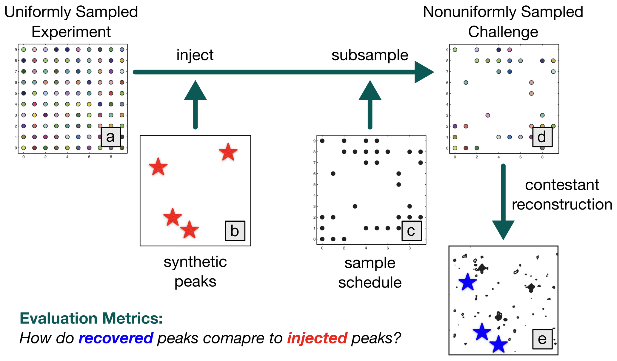
Figure 1NUScon workflow. The uniformly sampled experiment (a) is injected with synthetic peaks (b, red stars) and subsampled (c) to generate a nonuniformly sampled challenge data set (d). Contestants provide scripts to reconstruct the spectra (e). The recovered peaks (e, blue stars) are compared against the injected peaks (b, red stars) using a variety of metrics to determine spectral quality.
2.1 Challenges
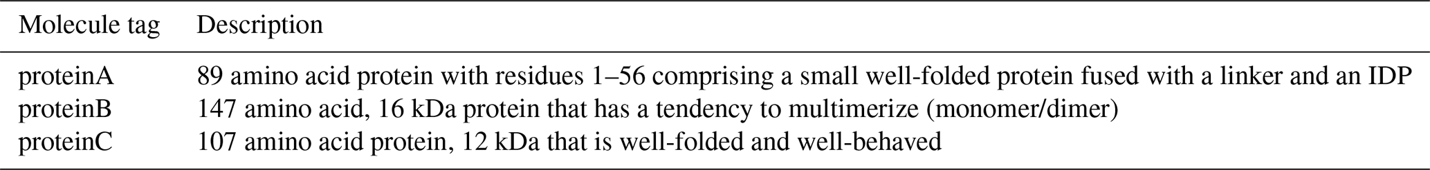
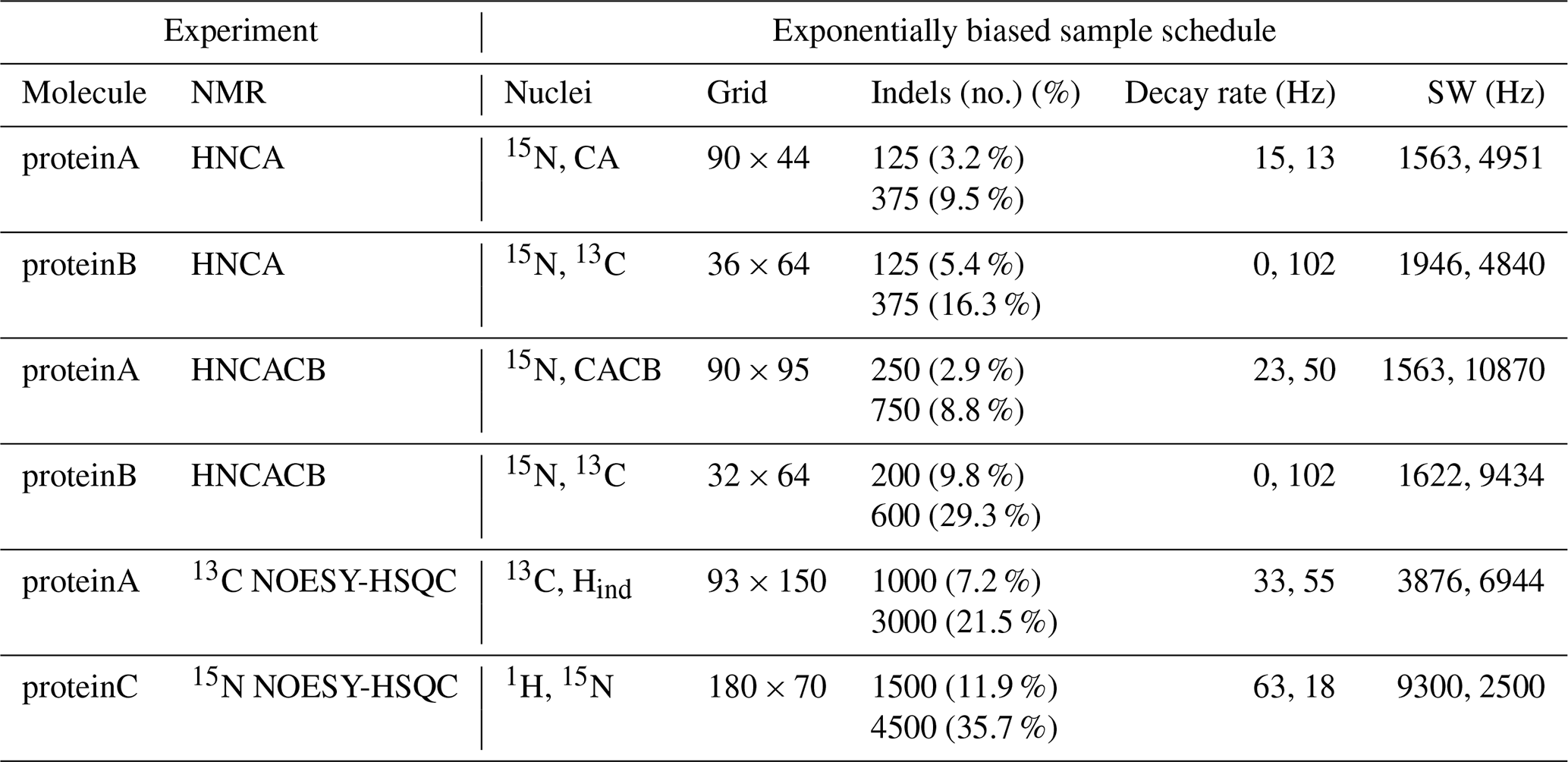
Each NUScon challenge began with an unpublished experiment that was collected with US. The Challenge Committee was tasked with identifying appropriate experimental data that are high quality and representative of molecular sizes and experiment types of interest to our community. The descriptions provided to the contestants for each molecule used in a challenge data set are given in Table 1. A configuration file was deposited with each experiment, which provided basic metadata (e.g., number of points along the indirect dimensions, spectral width, and region of interest to be extracted along the direct dimension) that were used by the processing workflow. An example configuration file is included in the Supplement. We also include 1H,15N projections from the 3D challenge data in the Supplement; these were not provided to contestants during the open challenge.
Table 1Descriptions provided to the contestants for each of the molecules used in the challenge data.
2.2 Synthetic peaks
Evaluating the performance of a spectral reconstruction method is a challenging proposition, especially if the procedure must be automated. The central challenge is that NMR spectra are used for many purposes, and the properties that make a reconstruction most fit for purpose are not always the same. Also, in practice, parameters of interest are generally extracted from spectra rather than from time-domain data. So, while it is possible to make an unbiased, automated evaluation of agreement between observed time-domain data and the corresponding time-domain version of a reconstruction, this does not necessarily capture how effectively a reconstruction may serve a particular spectral analysis task.
Along these lines, while it may be possible to measure fidelity of frequency, amplitude, and signal envelope (decay) of individual signals, this does not necessarily capture the fitness of a reconstruction to suit a given use. In particular, while NUS reconstruction methods can have excellent lineshape fidelity (Stern et al., 2002; Bostock and Nietlispach, 2017; Roginkin et al., 2020), it is seldom important in practice that a lineshape be conserved by a reconstruction, hence the common use of apodization that alters the lineshape, even if it conserves the integral (Naylor and Tahic, 2007). This is particularly true in multidimensional biomolecular data, where the indirect dimensions have little or no decay, so that the observed lineshape is primarily due to signal processing details rather than to any property of the underlying time-domain data. Furthermore, many applications, such as typical backbone assignment tasks, do not use peak heights or integrals quantitatively. Therefore, as a general point, it is often more useful to sharpen peaks or to suppress reconstruction artifacts than it is to faithfully reproduce lineshape.
The NUScon Planning Committee developed strong consensus that the single most important property of spectral reconstruction is for a real peak to be detectable, a fundamental requirement for all subsequent analyses. This, in turn, means that the evaluation of a reconstruction method is conflated with the procedure used to detect a peak. This is especially problematic for NMR, since the final decision about whether a spectral feature is a peak is often performed visually. Evaluation of the fidelity of the frequency, amplitude, and decay of a signal is likewise conflated with the procedure used to extract these parameters. The performance of such procedures is influenced by the presence and dynamic range of other peaks in the spectrum and by residual phase distortion, systematic artifacts, thermal noise, and the true functional form of the underlying NMR signals. Regarding this latter point, evaluations are further complicated by the potential for a single multidimensional peak to actually be a composite of mixed-phase signals in the presence of one or more unresolved couplings (Mulder et al., 2011) or the mixtures of signals with different relaxation pathways (Pervushin et al., 1997).
Keeping these challenges in mind, we developed a flexible procedure to automatically define and insert synthetic signals into existing time-domain data. These synthetic signals have a similar appearance and arrangement to signals in the original data. For example, signals in an HNCA spectrum will generally occur in pairs at the same 1H,15N chemical shift and will share the same lineshape in the 1H and 15N dimensions. Accordingly, the signal injection procedure provides options to specify how the synthetic signals should be placed relative to existing peaks. For example, we can specify that two synthetic HNCA peaks are inserted at a random 1H,15N position where no peaks exist anywhere in the original 3D data but also that these two peaks are placed at 13C positions that correspond to peaks elsewhere in the original data. In order to better mimic the appearance of measured data and to help minimize any evaluation bias due to use of synthetic data, the individual signals allow for random perturbations of linewidth and phase and optionally one or more random unresolved couplings in each dimension. It should be noted that there are opportunities to improve the realism of simulations still further, including using composite signals of mixed phases or linewidths or by attempting to match the coupling constants and decays of synthetic peaks to the values of related peaks in the measured spectrum. For example, in the current HNCA peak generation procedure, peaks can be inserted to align with a 13C chemical shift of a peak elsewhere in the measured spectrum, and that synthetic peak will have randomly chosen 13C decay and couplings. In a more realistic simulation, the synthetic peak could be generated to match not only the 13C chemical shift of a peak elsewhere in the spectrum, but also that measured peak's 13C decay and couplings, provided that these details are known.
The signal injection procedure automatically characterizes the experimental reference spectrum to prepare for the injection of synthetic peaks. The procedure was built from C-shell and TCL scripts using the facilities of NMRPipe and its custom TCL interpreter nmrWish (Delaglio et al., 1995; Johnson and Blevins, 1994; Ousterhout, 1994). Here, we present an outline of an HNCA example used in the first NUScon, with complete data and scripts available on NMRbox (Maciejewski et al., 2017). The input to the procedure was the measured reference 3D time-domain data, which were used to establish acquisition parameters used for simulating time-domain data, and the corresponding 3D spectrum, which was used to establish the phase values for simulated signals so that the simulated data can be processed by the exact same scheme applied to the measured data. The output of the procedure was a table of synthetic 3D signals, a 3D time-domain simulation with only the synthetic signals, and a version of the reference 3D time-domain data with the synthetic signals added.
-
The fully sampled 3D time-domain reference data are Fourier processed to generate a corresponding spectrum.
-
Automated peak detection (detection of local maxima) was applied, and the largest peaks were retained (256 peaks for this HNCA example). The NMRPipe peak detection procedure estimated heights and linewidths by a multidimensional parabolic fit of the points around the maxima.
-
Using knowledge of median linewidths from peak detection, each point in the 3D spectrum was evaluated to decide whether it was in an “empty” region, meaning that there are no substantial signals within ±2 median linewidths. The criteria are that the rms of the region must be below 1.15 times the estimated noise and that no points in the region are above 5.0 times the estimated noise. The results were saved as a mask of the 3D spectrum, where intensities were set to 1 for each point with an empty neighborhood and 0 otherwise. Two-dimensional projections of the 3D mask were also prepared as shown in Fig. 2.
-
Using the peak and mask information from the steps above, the utility
genSimTab.tclwas used to generate a synthetic peak table. Synthetic signals were only inserted in empty regions of the original data. Each row in the output peak table described one signal by a single amplitude and by a frequency, exponential decay, and phase for each dimension. Optionally, one or more couplings (cosine modulations) for each dimension may be specified. An example NMRPipe command illustrating the use ofgenSimTab.tclis shown in Fig. 3. A key feature ofgenSimTab.tclis that the desired properties of the signals to insert can be specified by a “program” of keywords and values, allowing substantial flexibility. Each program generates one or more “strips” (3D peaks at the same 1H,15N coordinate). For HNCA data, each strip of synthetic signals consists of two 3D peaks. For example, the programmeans generate one strip (
count=1) of two peaks (HNCA peaks are generated in pairs) at a randomly chosen 1H,15N location where no peaks exist anywhere in the original 3D data (xy=novel) but at 13C positions of known peaks elsewhere in the spectrum (z=existing). -
Synthetic time-domain data were generated by the
simTimeNDapplication using the synthetic peak table and the acquisition parameters from the measured data as inputs. This included the placement of a group delay of “negative time” points at the start of each 1D time-domain vector if the reference data did not properly account for digital oversampling, as is the case for data from Bruker spectrometers (Moskau, 2002). The synthetic signals had exponential decays, with options for mixed-time data (Ying et al., 2007). The synthetic data also included a synthetic solvent signal of fixed width whose amplitude, phase, and frequency varied randomly in each 1D time-domain vector according to specified lower and upper bounds. -
The synthetic time-domain data were added to the experimentally measured reference time-domain data. Example 2D projections and strip plots are shown in Figs. 2 and 4, respectively.
-
Given an appropriate sampling schedule, the fully sampled time-domain data can be resampled to generate NUS data via the
nusCompress.tclutility.
An advantage of this scheme is that it produces a spectrum processed identically to the experimental data but containing only synthetic peaks. This allows the simulated signals to be subjected to any desired detection or quantification method in either the presence or absence of signals and noise from the measured data.
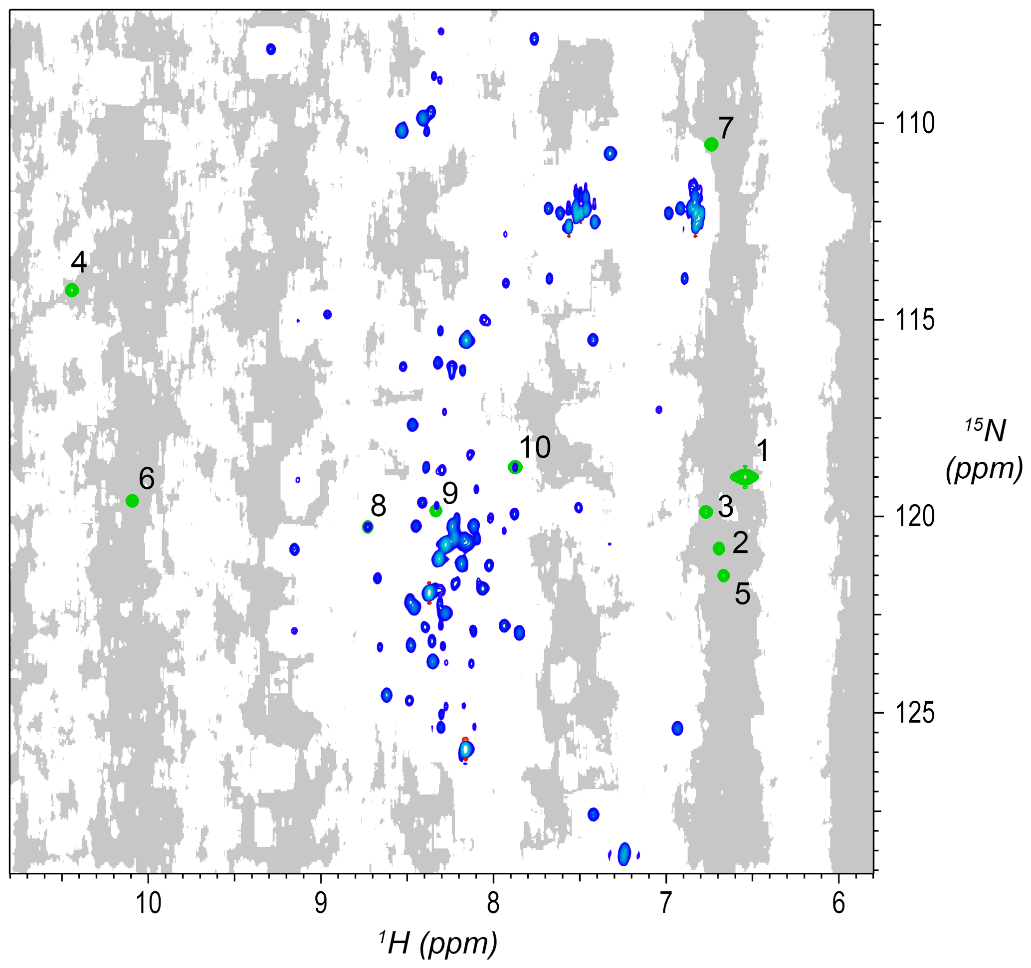
Figure 2Synthetic peaks injected into HNCA empirical data. Two-dimensional projection of the 3D empty region mask (gray) overlayed with the 2D projections of the 3D reference spectrum (blue) and simulated signals (green). The areas shaded gray are regions in the measured data determined to be signal-free, such that a signal inserted at any shaded position will have no substantial signals nearby anywhere in the 3D spectrum. Synthetic signals were generated by the command in Fig. 3, which generates 10 strips of synthetic peaks at the 1H,15N positions labeled here. Strips from positions 7 to 10 are shown in Fig. 4. As can be seen here, strips 1 to 7 are at 2D coordinates with no existing peaks, strip 9 is at a 2D coordinate that partially overlaps with existing peaks, and strips 8 and 10 are at 2D coordinates that correspond exactly to existing peaks.
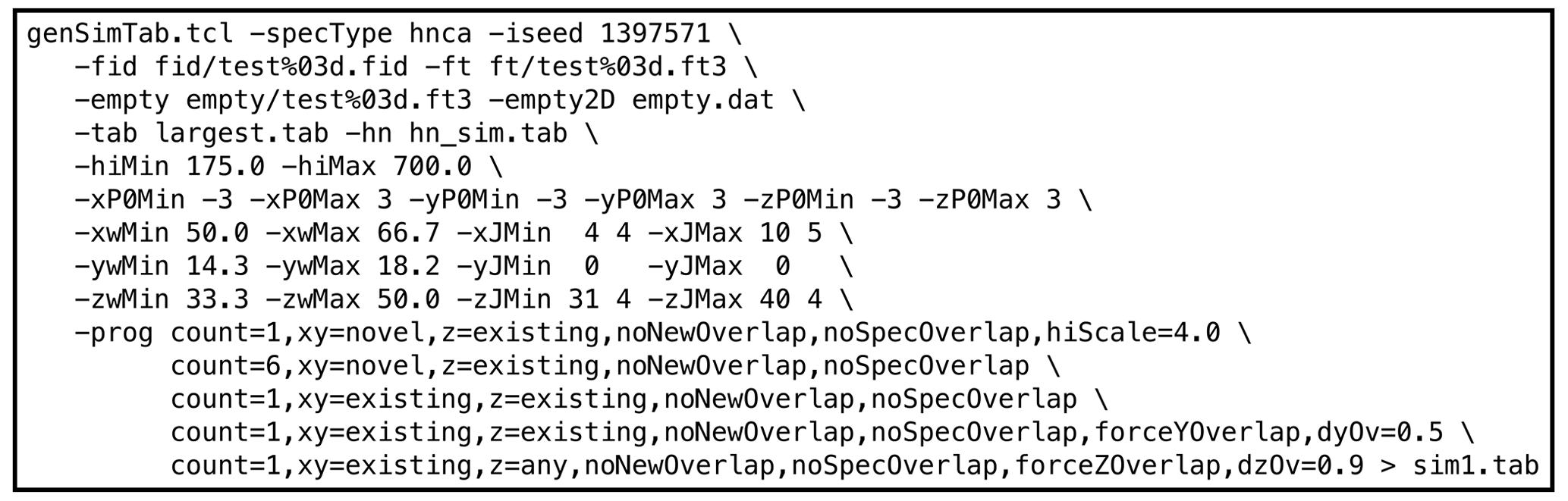
Figure 3Example genSimTab.tcl command. This command generates a table of synthetic peaks for an HNCA spectrum.
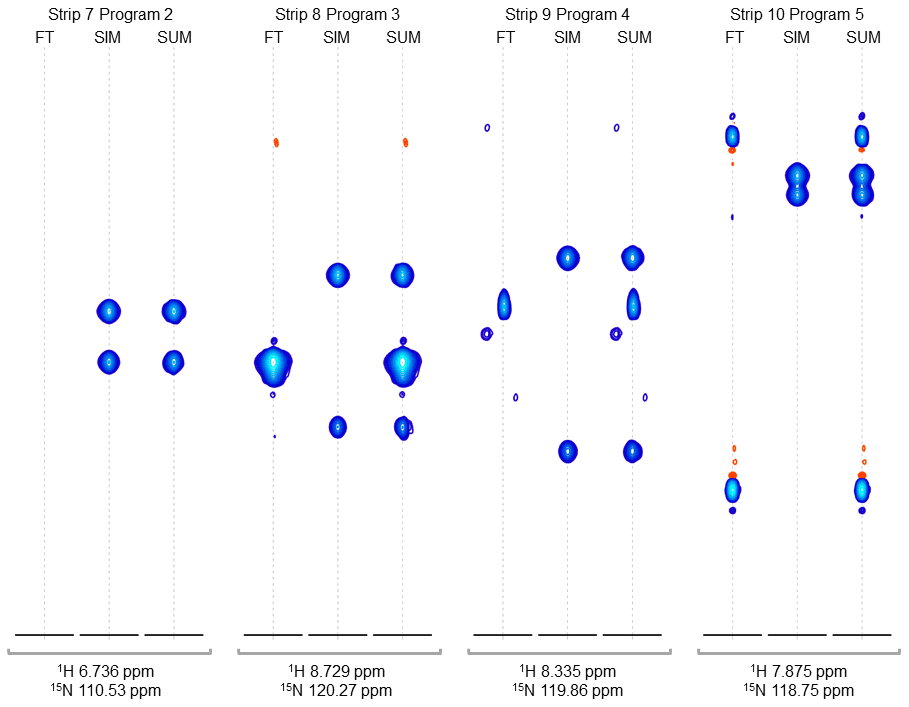
Figure 4Strip plots of synthetic peaks. These strips show the auto-generated synthetic peaks and the corresponding measured data from the command in Fig. 3. The command uses five “programs” to produce strips of synthetic 3D signals at 10 1H,15N positions. The last four groups of strips (groups 7 to 10) are shown here, from the measured spectrum, simulated spectrum, and sum, labeled FT, SIM, and SUM, respectively. For these HNCA data, two simulated signals are inserted in every case. Strip group 7 corresponds to a program which inserts signals at 1H,15N locations where there are no peaks anywhere in the original data, so that the “FT” strip in group 7 shows no signals. Strip group 8 corresponds to a program that inserts non-overlapping peaks at a 1H,15N position where there are signals at other 13C positions in the original data. Strip group 9 corresponds to a program that inserts peaks which are offset by 0.5 ppm in the 15N dimension relative to an existing peak in the original data. Strip group 10 corresponds to a program which inserts two peaks that are 0.9 ppm apart in the 13C dimension. It can also be seen that the measured data for this case have a combination of peaks with a broad appearance, as in FT strip 8, and peaks with a narrow appearance, as in FT strips 9 and 10.
2.3 NUS sample schedules
The NUScon software generates sample schedules by passing parameters to the nus-tool software package on NMRbox. The NUScon contest employed an exponentially biased sample schedule at a low and high coverage for each experiment. The parameters that defined each sample schedule are described in Table 2. The public archive of NUScon data contains the sample schedules along with the complete nus-tool command used to generate each schedule, including the random seed.
Table 2 has a column that shows the “grid” size, which is the dimensions of the Nyquist grid that spans the indirect dimensions. Following the notation established in Monajemi et al. (2017), each point in a sampling grid is an indel (indirect element). The column in Table 2 labeled “Indels” shows the number of indels that were collected by the corresponding sample schedule. Each indel represents four FIDs for these three-dimensional experiments with quadrature detection employed. All schedules used “full component sampling,” so all four FIDs were collected at each indel. In future work, we may consider partial component sampling (PCS; Schuyler et al., 2013), where the group of FIDs at each indel may be subsampled.
Table 2Challenge experiments and sample schedules. The left half of the table shows the NMR experiments that define each challenge data set. The right half of the table shows the sampling parameters used to generate a lower and a higher coverage exponentially biased sample schedule for each experiment. The column “Nuclei” lists the indirect dimensions, as specified in the fid.com scripts. The term “Indels” (i.e., “indirect elements”) is a single combination of evolution times taken across all indirect dimensions. Sample schedules customarily list the indels at which FIDs are collected. Dimensions that are constant time are indicated by zero-valued decay rates.
The nus-tool command to generate each sample schedule used input flags to force the collection of all FIDs at the “first” and “last” indels (i.e., the FIDs taken at the lowest and highest combinations of evolution times). The first indel, which contains the largest signal intensity, would very likely be sampled by any reasonable exponentially biased sampling schedule, but forcing its inclusion is an advantageous convention. The size of the Nyquist grid was explicitly defined in the NUScon workflow metadata. However, in practice, empirical data may not include such information, and the largest time increments observed in a sample schedule are often the best indicators of the size of the Nyquist grid. To comply with that convention, we forced the inclusion of the last indel.
2.4 Spectral reconstruction
We provided contestants with a template script for submission that accepts NUS time-domain data, a sample schedule, and various other parameters as inputs. Contestants were charged with using any of the tools on the NMRbox platform to process the data and produce a spectrum, subject to a basic set of rules. These rules include general guidelines, like the ethics statement “Any script that is not `reasonable' or tries to cheat the challenge problem is disqualified.” The rules also contain specific processing guidelines to ensure fair evaluations: “The spectrum produced by the user script must not exceed a final size larger than `rounding up' each dimension to the next Fourier number and 3 zero fills.” The rules document is available in the NUScon archive on NMRbox.
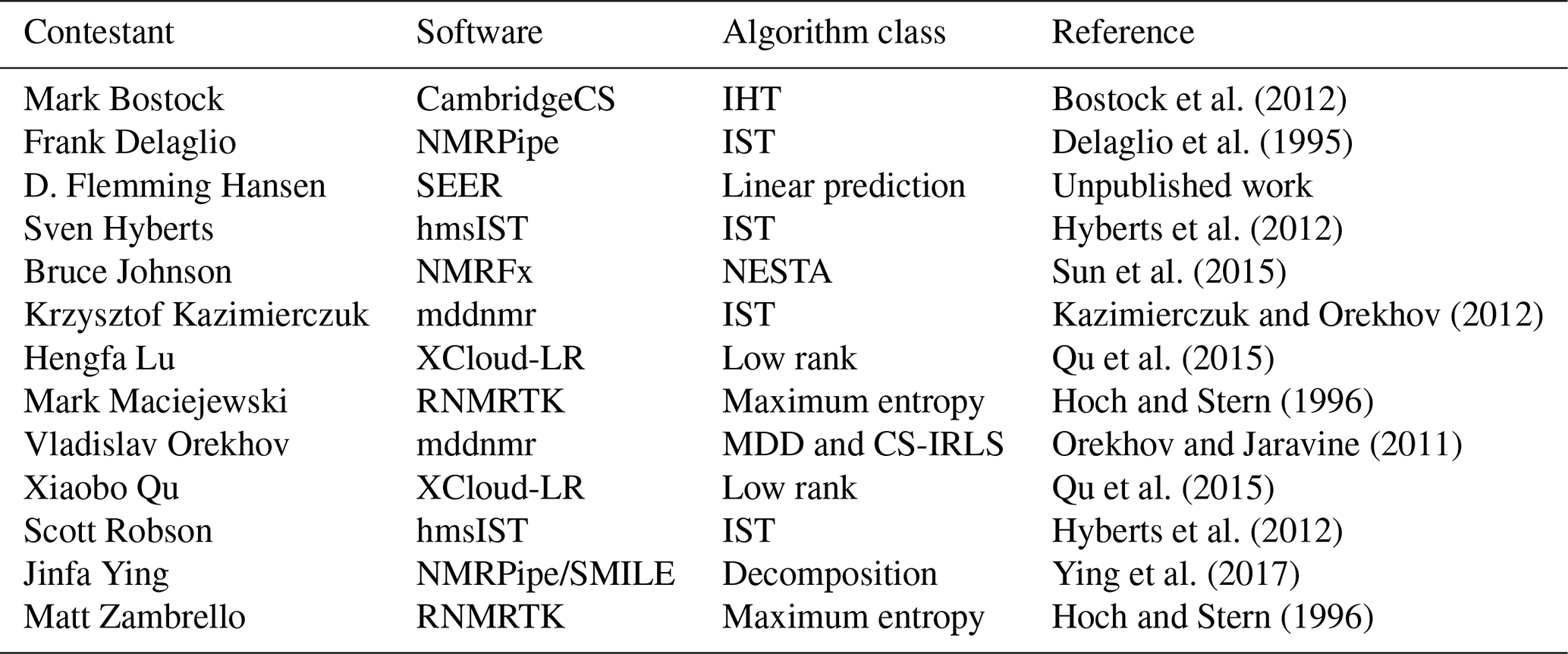
The range of reconstruction software programs employed is summarized in Table 3. Several of the software packages provide access to various reconstruction algorithms, and some contestants used different algorithms for different challenges. The specific methods and parameters used by each contestant for each challenge should be referenced directly in their submission scripts inside the NUScon archive. It is worth noting that the SEER (from Hansen) and low-rank (from Qu and Lu) software packages were new to NMRbox and were provided along with the contest submissions. This showcases the ability of the NUScon workflow to promote the exploration of novel techniques and the agility of the NMRbox platform to readily incorporate them.
Bostock et al. (2012)Delaglio et al. (1995)Hyberts et al. (2012)Sun et al. (2015)Kazimierczuk and Orekhov (2012)Qu et al. (2015)Hoch and Stern (1996)Orekhov and Jaravine (2011)Qu et al. (2015)Hyberts et al. (2012)Ying et al. (2017)Hoch and Stern (1996)Table 3Contestants and categorization of their chosen spectral reconstruction methods.
2.5 Peak picking
The peak picking step in the workflow was simple to deliver but deceptively complex to interpret. We used the peak picker from NMRPipe, but setting the threshold and controlling the number of peaks recovered required some attention. The recovered peak table was used by the metrics discussed in the next section and, as will become clear, the number of peaks in the recovered table had an effect on the resulting metrics. As a consequence, the threshold used when peak picking had a direct effect on the metrics. Given that NUS reconstruction methods are nonlinear, there is no single intensity threshold that can be used across all reconstructions for a given data set. Therefore, the peak picking was performed with a low threshold; the resulting peak table was sorted by peak intensity and truncated to include 1500 of the most intense peaks. The fixed number was determined by manual inspection of the uniformly sampled empirical data and was set conservatively high to ensure that all true peaks would be captured.
The current approach based on a fixed number of recovered peaks was effective but will be replaced by the use of the in situ receiver operator characteristic (IROC, Zambrello et al., 2017) method in future rounds. The IROC method is advantageous since it continuously varies the peak picking threshold from the most intense peak down to the noise and reports the recovery rate and false discovery rate at each threshold. The resulting set of data defines the quality of the reconstruction independently of a specific peak picking threshold.
2.6 Metrics
The NUScon metrics were designed to quantify how well reconstruction workflows recover synthetically injected peaks. The metrics are briefly described here, and their full mathematical definitions are presented in Appendix A.
-
M1: frequency accuracy. A symmetric Hausdorff metric was used with a maximum distance penalty to determine the accuracy of the recovered chemical shift positions. This metric allowed for different numbers of peaks in the injected and recovered sets (i.e., it does not require a one-to-one correspondence between the sets).
-
M2: linearity of peak intensity. This quantifies how well the intensities of the recovered peaks were mapped by a linear function to their corresponding injected intensities. The correlation coefficient was calculated from the NumPy python package.
-
M3: true positive rate. This reports the percentage of injected peaks that were recovered.
-
M4: false positive rate. This reports the percentage of recovered peaks that were false.
-
M5: linearity of peak intensity. This metric delivers the same evaluation as M2 but was implemented using an NMRPipe function.
2.7 Rank lists
A rank list was generated for each metric applied to each combination of experiment data, synthetic peak table, and NUS schedule. These rank lists are in the NUScon archive on NMRbox in comma-separated value (CSV) files. The report function in the NUScon software package can be used to extract arbitrary subsets of these rank lists to assemble aggregate results, which is how the NUScon challenges were evaluated.
The NUScon software package is a modular, workflow-based, python3 software package that is installed on the NMRbox platform (Maciejewski et al., 2017). NMRbox accounts are freely available to those with academic, government, and nonprofit affiliations. The NUScon software is licensed with GPL3. Users may run the software on NMRbox by executing the command nuscon, access the source code in /usr/software/nuscon, or import the NUScon python package into their own projects. NMRbox users can also execute the command nuscon -h to see a help message that defines input syntax and provides information about auto-generating a template file to run NUScon jobs. This publication uses NUScon software version 5.0.
The NUScon software was designed to manage a collection of project directories that contains the US experiment data, synthetic peak tables, sample schedules, and user submission scripts. As each evaluation was performed, workflow output was written to project directories that contain the spectra, projections, and peak tables. In addition, a JavaScript Object Notation (JSON) file was written to the output directory for each reconstruction that documented the metadata that defined the particular reconstruction, the compute times for each task in the NUScon workflow, and the metric scores. When rank lists were generated, the software simply queried the JSON files to aggregate all scoring data needed for the report. Compartmentalizing all of the workflow resources into nested project directories made it easy to run the NUScon workflow in parallel across the NMRbox computing cluster and to extract arbitrary subsets of evaluation data from the NUScon archive by experiment, user, metric, etc. JSON files are human-readable and contain a nested structure of key–value pairs. JSON files are easy for users to browse, efficient for computing workflows to parse, and straightforward to augment as new evaluation tasks may be retroactively performed on existing data.
It is worth noting that the design of the NUScon software made it trivial to deploy across the NMRbox cluster for parallel computing. Since each virtual machine (VM) in the NMRbox cluster has its own scratch disk, NUScon operations that were file input and output intensive saw tremendous performance improvements. All NMRbox VMs connect to the same file system, so the parallel jobs were written back into a common project. The NUScon software includes a status utility that reports on the progress of each evaluation task defined in the project.
The Supplement shows examples of the input configuration files and an output JSON file.
A very generous gift from the Miriam and David Donoho Foundation allowed us to provide significant cash prizes to the contestants of the 2018 and 2019 challenges. This seed money provided incentive for the leading users and developers of the most prominent NUS software to participate, with the goal of ushering NUScon into a community-driven initiative that is self-sustaining. The publicly available software package is the first deliverable presented here, and the remainder of this section addresses the utilization of the software package to support two rounds of challenge problems.
Varying the type of experiment, nature of the synthetic peaks, sample schedule parameters (including coverage and random seed), and the metrics allowed for a comprehensive analysis of spectral reconstructions. It is important to note that while we customize the properties of the synthetic peaks for use with each metric, there are compounding factors to consider. When peaks are weak, broad, and/or close in proximity to additional peaks, they become difficult to recover. In particular, their sensitivity, frequency accuracy, and resolution are intimately connected, and quantitatively isolating any single property becomes challenging. We strive to minimize these complicating factors in our evaluation workflow by using a variety of synthetic peak collections for each experiment; the -prog section of the command in Fig. 3 defines five different strips of synthetic peaks. Strong synthetic peaks in closely spaced pairs are employed to assess resolution, strong peaks in isolation are used to evaluate frequency accuracy, and variable intensity peaks in isolation are employed to measure sensitivity.
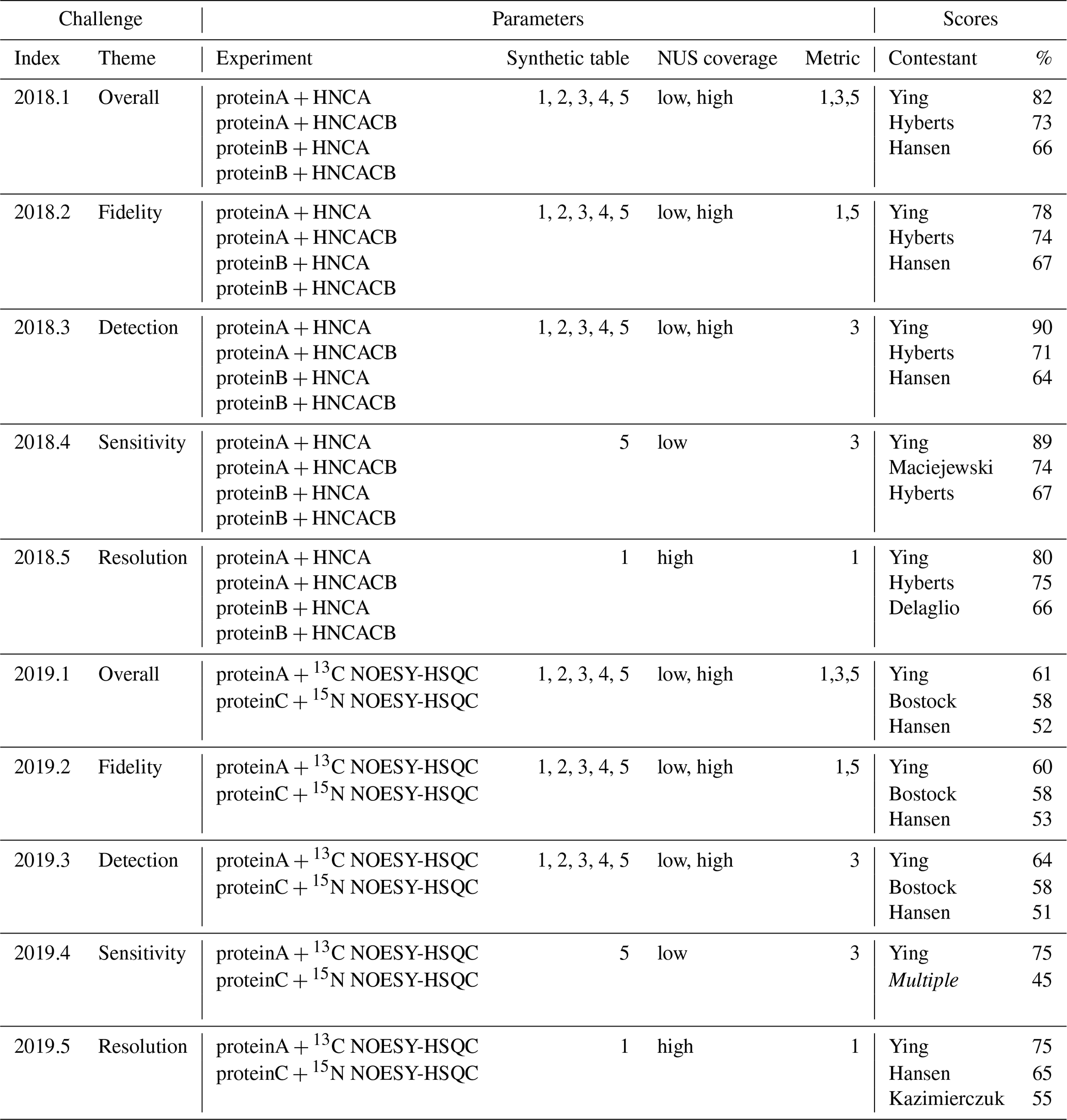
In the context of NUScon, it was desirable to combine the scoring results for multiple data sets in order to evaluate each of the challenges, as summarized in Table 4. Since all metrics are normalized onto the interval [0,1], it may be tempting to combine multiple metrics through averaging. However, the dynamic range of each metric is hard to pre-determine, and thus a mean score would be dominated by whichever metric had the largest range of values. Instead, we chose to rank order all submissions for each metric on each data set, converted these ranks into percentiles (i.e., a representation that is independent of the number of contestants), and then combined results by averaging the percentiles. This approach has the consequence that adding new evaluation scripts to the archive of existing challenges requires the re-scoring of the percentiles for all evaluations. Computationally this is insignificant, but it is worth noting that percentile rankings are dependent on their context, whereas the raw scores will remain unchanged and are a better choice for running iterative optimization.
Table 4NUScon challenges 2018/2019. Each row group (separated by horizontal lines) shows a NUScon challenge and the parameters that define it: “Experiment” defines the molecule and NMR experiment providing the uniformly sampled time-domain data. “Synthetic table” gives the index value(s) of the five synthetic peak tables that are generated for each experiment (see the Workflow discussion for information about the design of each). “NUS coverage” indicates the usage of the “low” and “high” coverage sample schedules generated for each experiment, as defined in Table 2. “Metric” lists the index value(s) of the metrics used to evaluate the reconstructions (see the Workflow discussion for information about each metric). The “Scores” column shows the top-performing contestants for the given challenge along with their average percentile taken across the evaluations of all parameter combinations that define the challenge. Note that not all contestants provided a submission for each challenge. The entry “Multiple” indicates a tie; complete results available in the NUScon archive.
Another consequence of using rank order is that a difference in rank may result from either a small change in the underlying raw scores when many contestants are tightly grouped or from a large change in the underlying raw score when contestants are well-separated. The former may be insignificant, whereas the latter may indicate an important difference in performance. As an illustrative example, consider an alternative version of metric M1 that computes differences in peak positions in parts per million (ppm) rather than in Hertz. This approach resulted in small changes in the raw scores, which in many of the challenges resulted in a shuffling of the ranked results. This example suggests one be cautious not to over-interpret the ranked results in Table 4.
The parameter combinations that defined each NUScon challenge are given in Table 4. The NUScon archive inside NMRbox at /NUScon/archive/report contains CSV files showing the rank lists by contestant for each metric on each data set. There are also CSV files showing the aggregated ranked results for each of the challenges shown in Table 4. Note that not all contestants provided a submission for each challenge; the CSV files of rank lists should be consulted to determine participation in each challenge. It is also important to note that the “Scores” column in Table 4 should be cautiously interpreted; it should not be used as a way to select a best reconstruction algorithm for an arbitrary experiment, and it should not be used to eliminate a reconstruction method from consideration. The challenge experiments, synthetic peaks, contestant reconstruction scripts, and metrics represent a diverse collection of data that will guide the community towards best practices. However, the collection is still a slice through a very complex workspace. We intend to expand the scope of NUScon and to continually refine the evaluation metrics through future rounds of challenges. This follows the successful framework used in CASP (Kryshtafovych et al., 2019) and will help drive our evolving understanding of the challenges we face with NUS NMR.
The summary of computations performed for NUScon is provided in Table 5. These data are provided as a qualitative way to describe the overall computational costs of the NUScon challenges. Direct comparison of compute times between various methods is beyond the current scope of the project and would depend on the optimization of each method to run multi-threaded operations. In addition, the NMRbox platform is a shared community resource with active users. The NUScon evaluations were performed in this dynamic environment where resource availability fluctuates.
Table 5Summary of computations. The number of spectral reconstructions and the compute times they required. Most of the reconstruction methods are multi-threaded, and all computations are spread across 10 NMRbox VMs to yield a substantial reduction in the “wall time” for completing the evaluations.
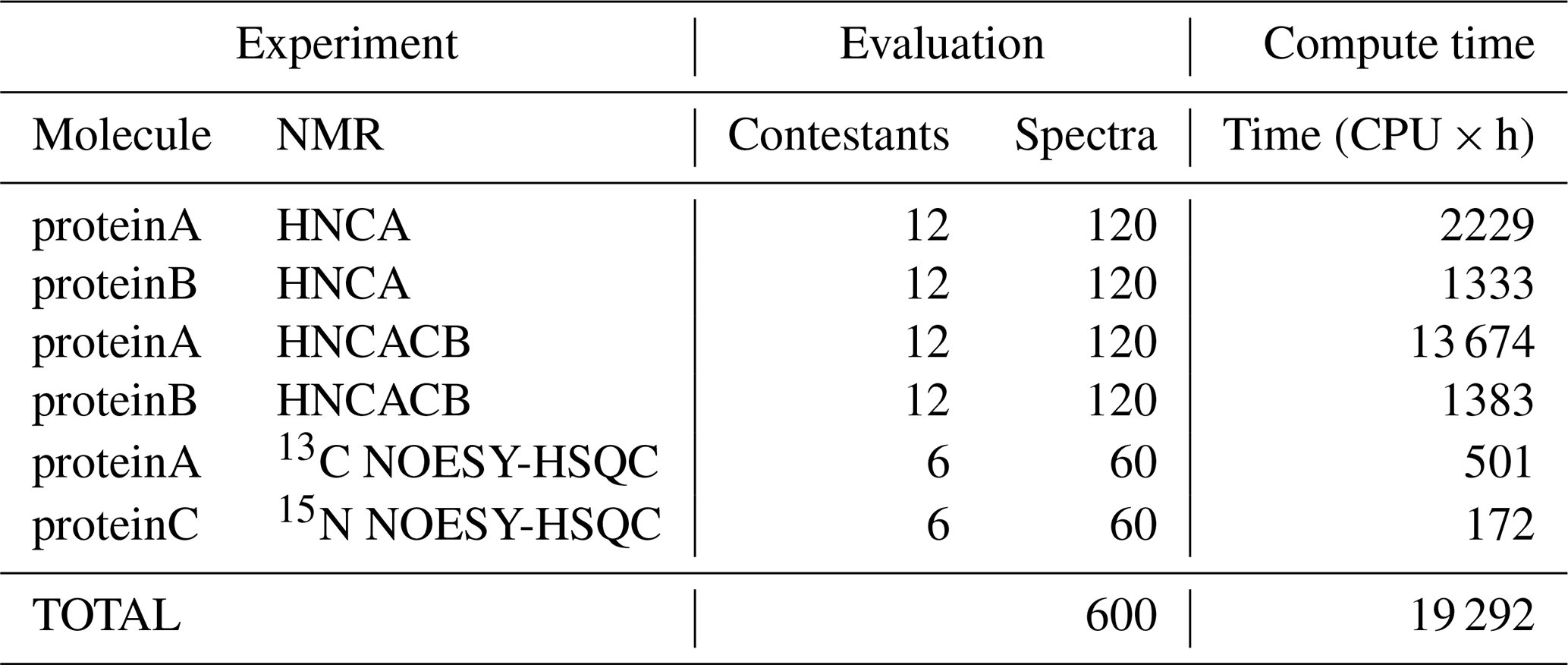
It is important to note that M2 was not used in the NUScon evaluation; M5 was used instead. M4 will not be used until IROC methods are incorporated (discussed in Conclusions). The number of peaks recovered was held constant, and M4 was thus redundant to M3. Rather than reducing the set of metrics supported by the NUScon software, we instead intend to support an arbitrary variety of metrics and welcome contributions from the community.
To ensure that the metrics were robust, we performed visual inspection of spectra to validate that differences in metric performance corresponded to expected differences in spectral quality. This ensured that future efforts to optimize reconstruction methods can be based on maximizing metric performance. Figure 5 shows a side-by-side comparison of the best and worst performers for each metric for the protein A/HNCA challenge data. Row 1 shows a spectral region with two synthetic peaks, which are indicated by the intersections of the labeled vertical and horizontal lines. Panel a shows a reconstruction that displays some distortion and inaccuracy in the recovered peak positions (M1 score = 0.01), whereas panel b shows an improved recovery of peak position (M1 score = 0.10). Row 2 shows a spectral region with two relatively weak synthetic peaks. Panel c shows a reconstruction that fails to recover one of the peaks (M3 score = 0.10), and panel d recovers both peaks (M3 score = 0.85). Row 3 shows a scatter plot of the recovered peak intensities versus their injected intensities. Panel e has a broader spread as well as a fairly intense peak that is not recovered (data point on the horizontal axis), resulting in a poor correlation (M5 score = 0.40). Panel f shows a reconstruction with a better linearity of intensities (M5 score = 0.99).
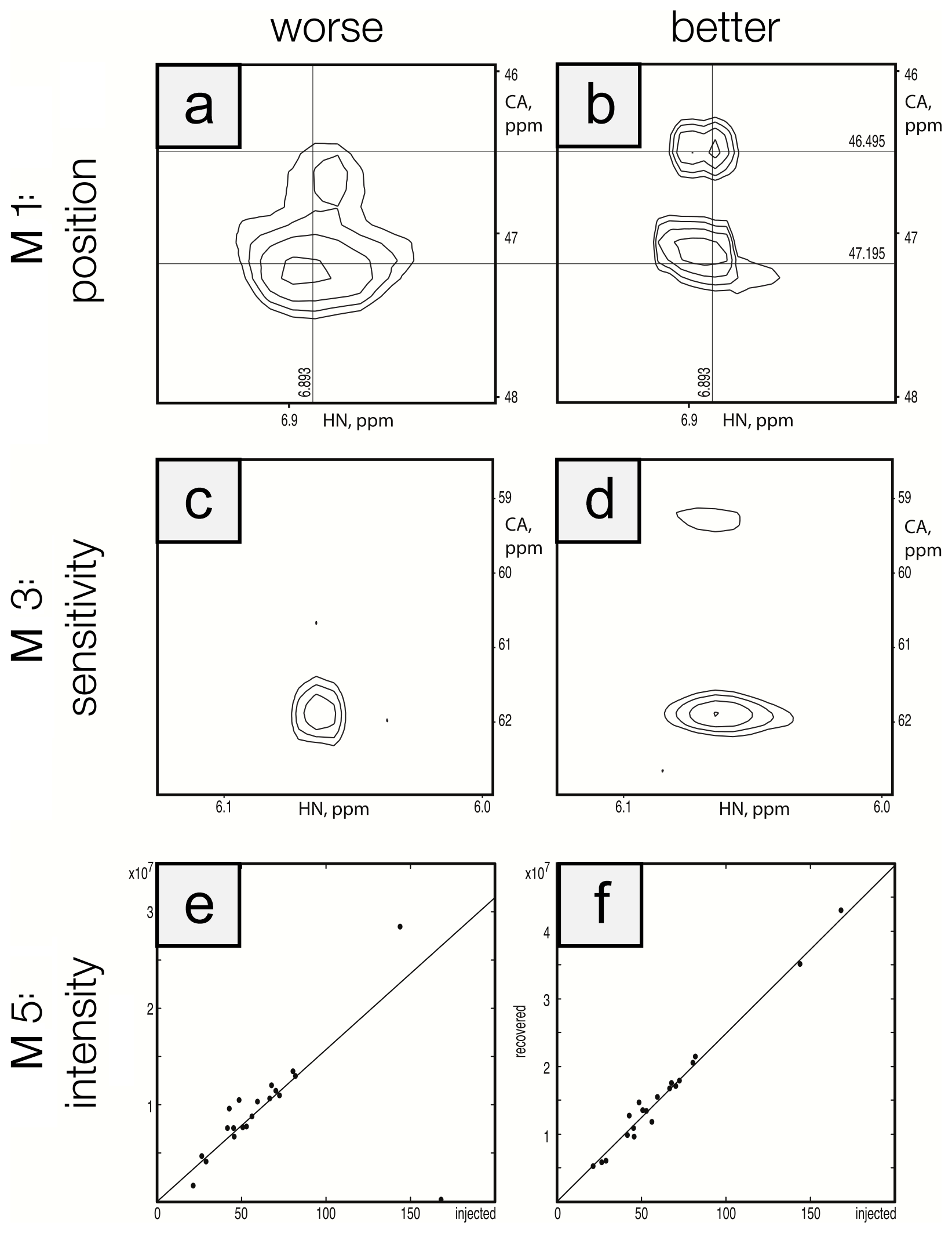
Figure 5Visualization of metric performance. Reconstructions that perform relatively worse (a, c, e) and that perform relatively well (b, d, f) are shown for each of the metrics M1 (row 1), M3 (row 2), and M5 (row 3) on the protein A/HNCA challenge data. The crossing lines in panels (a) and (b) intersect where a pair of synthetic peaks has been injected. The peaks in panel (a) are clearly offset and distorted. Panels (c) and (d) show a pair of weak peaks, only one of which is recovered in panel (c). Panels (e) and (f) show correlations between injected and recovered synthetic peak intensities.
The NUScon software, contest, and archive of spectral evaluation data provide a comprehensive platform for addressing the most challenging questions related to NUS experiments and even to broader topics in the quantitative analysis of NMR data. Establishing both a standardized workflow and a set of curated reference data holds tremendous power for the robust quantitative assessment of current methods and provides benchmarks by which novel methods may be compared and optimized. The NUScon workflow will expand in scope as new challenges are addressed (e.g., sample schedule design and peak picking), and the quantitative modules deployed in the workflow (e.g., metrics and peak simulation) will be subjected to continuous refinement.
A critical component of the NUScon workflow, which also has significant impact beyond the workflow presented here, is the genSimTab.tcl synthetic peak simulation package that Frank Delaglio delivered as an extension to NMRPipe (Delaglio et al., 1995). As discussed in the introduction and clearly presented by Donoho and Tanner (2009), quantitative evaluations of spectral reconstructions require that candidate peaks (i.e., the synthetic peaks used here as a “ground truth”) be surrounded by other spectral data of suitable complexity and density. The synthetic peak simulation package was custom built to specifically deliver these needed features for the NMR experiments addressed in NUScon challenges. The package is extensible and can readily be maintained to support future challenges.
Peaks in a spectrum generated by conventional discrete Fourier processing will include truncation artifacts and the effects of any window function applied. This means that peaks in a discrete Fourier spectrum will never actually be simple ideal functions, such as Lorentzians, even though such simple functions can often be good approximations of observed lineshapes. In addition, measured NMR signals will deviate from ideal behavior in other ways, such as in the case when sample instabilities occur (Gołowicz et al., 2020). The NUScon approach injects time-domain signals with known parameters into measured data and tests how well the injected signals can be recovered by the reconstruction method being evaluated. The synthetic time-domain signal injection approach, despite its advantages, comes at the price of a potential bias that was extensively discussed during the planning of NUScon. The synthetic signals are generated using ideal exponential decays, but several adjustments are applied in order to more effectively mimic experimental distortions. These adjustments include application of small random phase distortions, small random unresolved couplings, and addition of a synthetic solvent signal to induce baseline distortions. The simulated signals can also include placement of a group delay of “negative time” points at the start of each 1D time-domain vector to account for the potential distortion introduced by digital oversampling (Moskau, 2002). Even with these attempts to generate more realistic simulations, since the signal injection procedure uses signals with ideal exponential decays as a starting point, this might still favor parametric reconstruction methods that use the same ideal model without conferring this benefit on non-parametric reconstruction methods.
The results captured in our archive of spectral reconstructions have shaped our preliminary definition of best practices and provide a quantitative benchmark. Future challenge problems (scheduled to be released annually in September/October, with results showcased at the Experimental NMR Conference in March/April) will enable us to build a database of quantitative evaluations across the entire NMR data processing workflow. We have thus far focused on NUS data reconstructions for common triple-resonance experiments used in protein NMR. We plan to expand the workflow by releasing challenges that address sample schedule design and peak picking. We plan to expand the scope of the contest to include data processing for experiments on small molecules, where the performance of the algorithms observed here for 3D protein NMR experiments may differ and require alternate optimization. We plan to offer challenges on 4D experiments where quantitative guidance in the description of best practices has great potential to significantly reduce experiment time and improve spectral quality for a class of powerful but under-utilized experiments. The reconstruction methods included in this work are among the most heavily used, but there are numerous other approaches. We plan to solicit submissions from developers, and we will initially focus on emerging tools in the area of machine learning. The modular design and open access to the NUScon platform provide an easy mechanism for integrating novel tools into the NUScon workflow, where they can be retroactively applied to all previous challenge data.
There are several features that are in development and scheduled for release during the next round of challenges. The first major planned development is the incorporation of the IROC method into the peak picking task; this will eliminate the need for an arbitrary peak picking threshold. We have written the IROC functionality into a stand-alone API and wrapped this using the Common Workflow Language (CWL, Amstutz et al., 2016) – a framework for defining analysis workflows.
The second major planned development is to provide the NUScon software with distributed computing capabilities. This is currently managed by manually running batches of evaluation tasks on various NMRbox virtual machines. However, NMRbox has an instance of HTCondor installed, and we will provide a mechanism to easily run distributed and balanced computing jobs on the NMRbox cluster. One possible approach is to wrap the entire NUScon workflow in CWL and make use of emerging high-throughput management systems like REANA, which has direct support for connecting CWL to HTCondor (Mačiulaitis et al., 2019).
The final major planned development is the implementation of a GUI front end, which will assist users with building NUScon evaluation jobs and browsing the database of quantitative results.
The notation in Table A1 is used in defining the metrics.
Table A1Metric notation. These symbols are used to define the quantitative functions for the evaluation metrics.
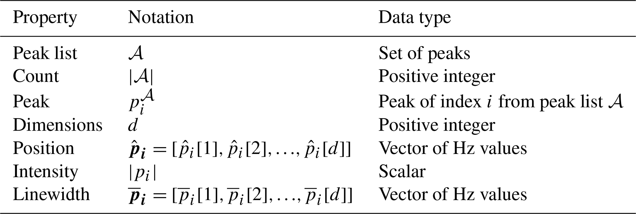
Note that subscripts are used to denote indexing of peaks and that square brackets are used to reference values specific to each dimension.
A1 M1: frequency accuracy
In order to quantify the frequency accuracy of a list of recovered peaks (ℛ) relative to a list of master peaks (ℳ), we need a method for computing the “distance” between peak positions. While it is trivial to compute the distance between pairs of peaks, it is not trivial to assign the pairings when the two lists may have different numbers of peaks due to artifacts, inadequate resolution, or low sensitivity; this is compounded when nearest neighbors are not mutual.
For example, consider Fig. A1, which depicts four master peaks (circles)
and three recovered peaks (squares)
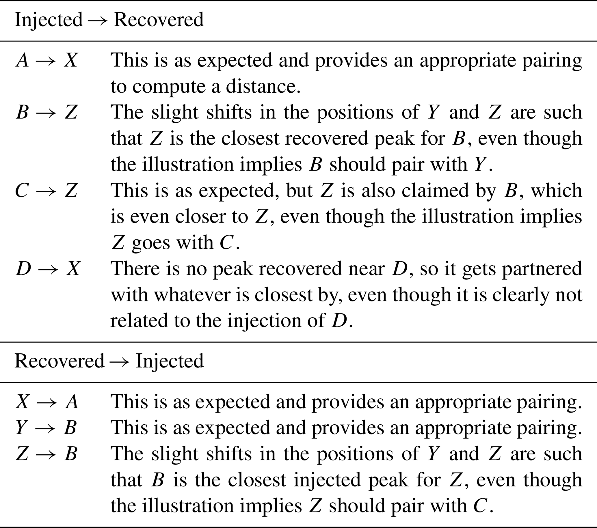
This illustration is meant to represent a case where three of the master peaks are recovered, but at slightly offset positions (A→X, B→Y, C→Z), and a fourth master peak (D) is not recovered at all. Table A2 shows the recovered peak that is closest to each master peak and vice versa (note that correspondence is not always mutual, hence the bi-directional assignments). In comparing the two assignment tables, we see a variety of situations.
-
A and X are mutual partners.
-
B and Z are mutual partners.
-
C selects Z, but Z selects B, which is also selected by Y.
-
D has no appropriate partner and selects X, which is clearly paired with A.
-
No injected peak selects Y.
-
No recovered peak selects C.
We account for the situations depicted above by using a symmetric Hausdorff distance, which considers the correspondence problems from both directions (and takes the average distance). We also include a maximum penalty term to guard against the distance penalty on D being highly dependent on the surroundings. This metric is formally defined as
The root-mean-square deviation (RMSD) obtained by selecting each peak in ℳ and finding its closest neighbor in ℛ is computed as
The function used to compute the distance between two arbitrary peaks, p1 and p2, is defined as
The first term in the “min” statement is the ℓ2 norm, which computes the distance (Hz) between peaks p1 and p2. The second term in the “min” statement, δmax, puts an upper bound on the distance and ensures that if the metric is used to compare two peak lists, a missing peak does not introduce an arbitrary distance term according to whatever is closest. The max value enforces a neighborhood around each peak when assigning correspondence. For each experiment, the table of synthetic peaks is used to establish an average linewidth along each dimension. These average linewidth values define a box, and the distance from the center of the box to a corner is used as the cutoff. In other words, the neighborhood around a peak position extends half a linewidth along each dimension.
The values of the symmetric Hausdorff distance in Eq. (A3) fall on the interval [0,δmax], with 0 indicating a perfect recovery of peak positions and a value of δmax indicating that no injected peaks have a recovered peak within the cutoff distance. This is normalized onto the interval [0,1] and reversed, so that 1 reports perfect recovery and 0 reports no peaks recovered, as
It is important to note that there are several ways to compute distances between peaks. We have chosen to perform this evaluation with peak positions in Hertz. Another approach we considered is to perform the computations in ppm and include weighting factors along the dimensions. Without this weighting, a 1 ppm difference along a proton dimension would be equivalent to a 1 ppm difference along a nitrogen dimension. In this example, it would be appropriate to use a weighting factor of c=1 for the nitrogen dimension and roughly c=0.25 for the proton dimension (Williamson, 2013).
A2 M2: linearity of peak intensity
The intention of this metric is to quantify the linearity of the peak intensities recovered by a reconstruction relative to the known intensities from a synthetically injected peak list. This metric assumes that the recovered peaks are limited in neither sensitivity nor resolution and that the correspondence of peaks between ℳ and ℛ is clearly defined. That is, the peaks are detectable above the noise, not overlapping, and the same indexing can be used to refer to both sets.
Let a set of n peaks from ℳ and ℛ be denoted as
where is the recovered peak corresponding to the master peak . The intensities of the peak lists are given as the vectors
The Pearson correlation coefficient is computed as
The correlation coefficient is on the interval , where the sign indicates a positive/negative correlation and the magnitude indicates the strength of correlation. This is converted to a value on the interval [0,1] as
The metric as defined above is computed using the Numerical Python (NumPy) library function numpy.corrcoef.
A3 M3: true positive rate
It might be tempting to simply count the number of peaks in ℛ that are within a cutoff distance of a peak in ℳ or count how many peaks in ℳ have a peak in ℛ within a cutoff distance. However, these approaches would allow a peak from one set to be considered a neighbor to multiple peaks in the other, thus artificially raising the count. We approach this metric by framing it as a bipartite graph, where the two peak lists form the two sets of vertices and the edges connect peaks from ℳ to peaks from ℛ that are within the cutoff distance (δmax), as defined in metric 1. The metric is then equivalent to finding the cardinality of a maximal matching on the bipartite graph (i.e., the most number of pairings between ℳ and ℛ where peaks are in at most one pairing). We solve this problem using the networkx module in python. We denote a maximal matching as
We denote the true positive rate as the percentage of master peaks that appear in the maximum matching
A4 M4: false positive rate
This metric reports on the rate of false positives in the recovered peak list. The false positive rate, which is defined as the percentage of peaks from ℛ that do not correspond to a master peak, is obtained as
This rate is on the interval [0,1], but the best performance (i.e., no false positive peaks in ℛ) corresponds to a value of 0. The output of the metric can be simply reversed, so that the best performance is at a value of 1 and the worst is at 0. This is done by subtracting the false positive rate from 1, producing
A5 M5: linearity of peak intensity
This metric uses the NMRPipe function pkDist.tcl to compute the Pearson correlation coefficient comparing the heights of synthetically injected peaks with the heights of the recovered peaks. This function establishes a correspondence between each injected peak and the closest corresponding recovered peak. This metric should be employed on synthetic peaks that can clearly be recovered in order to avoid an ambiguous correspondence between the recovered and injected peaks. The correlation coefficient is defined on the interval −1 to 1, but it would not be plausible to observe a negative correlation for the way this metric is deployed. As such, the reported M5 metric is simply the correlation coefficient.
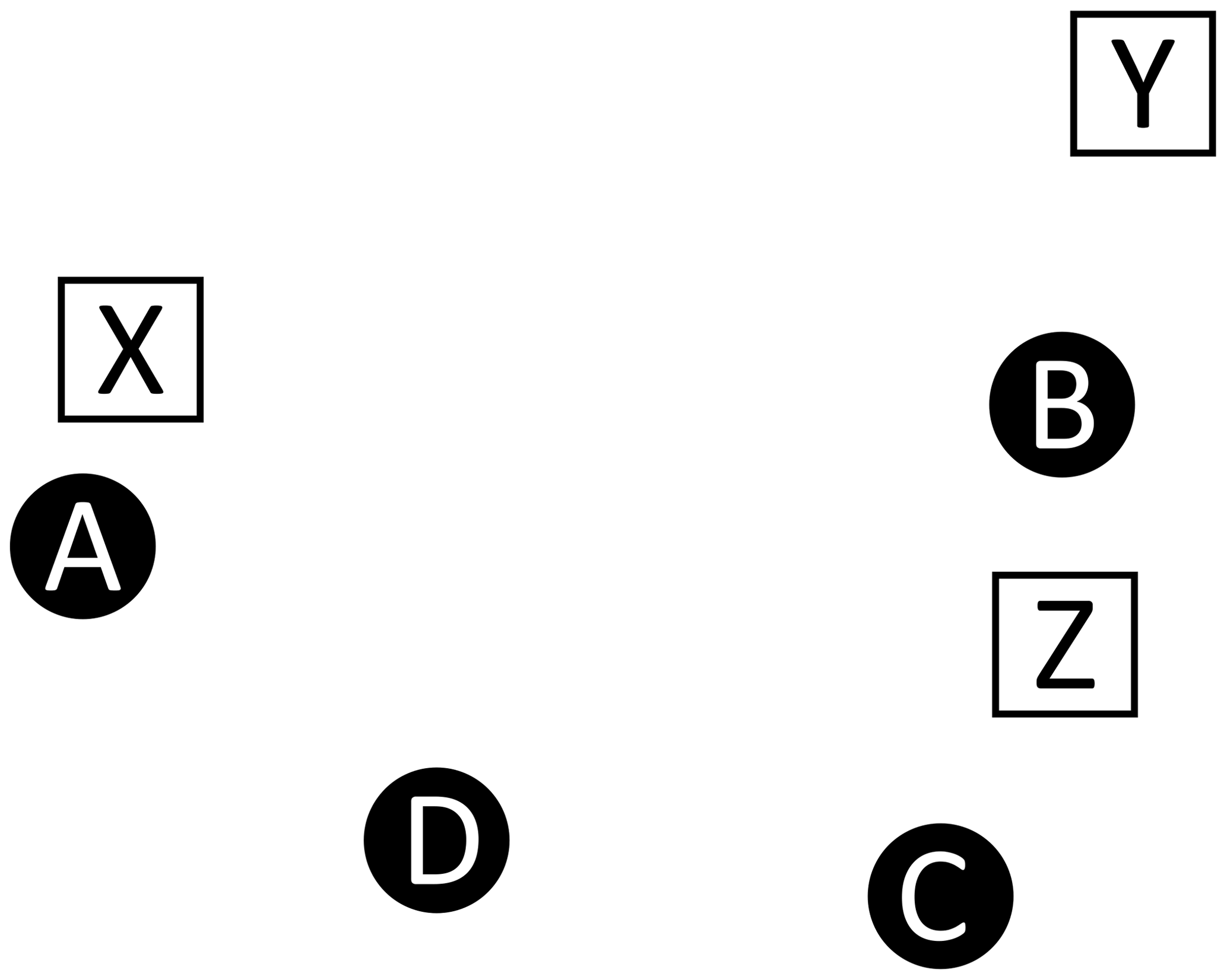
Figure A1Correspondence. This example illustrates a case where recovered peaks (white squares) are slightly offset from the injected master peaks (black circles). One injected peak (D) is not recovered and the offset introduces challenges relating to the correspondence between the two lists, as described in Table A2.
Table A2Correspondence. This table describes Fig. A1, by listing how each of the injected peaks is mapped to their closest recovered peak. This mapping is also performed in the reverse direction, as correspondence assignment is not mutual.
We dedicate this publication to Nobel Laureate Richard R. Ernst for his extraordinary contributions to what we recognize as modern, high-resolution NMR. Ernst's development of pulsed NMR and subsequent usage of the Fourier transform improved the sensitivity of the technique by orders of magnitude, which opened up new applications across the biological and physical sciences. He revolutionized the field again with his contributions to the development of multidimensional experiments, which enhanced resolution and made the study of larger and more complex molecules possible. These monumental advances emerged in concert with the increasing power and availability of computational resources, leading Ernst to declare, “Without computers – no modern NMR” (Ernst, 1991). The NUScon community continues in this spirit of discovery and gratefully acknowledges him.
The NUScon software package (nuscon v5.0) is installed on NMRbox, and all contest data are archived and available on NMRbox at the mount point: /NUScon.
The supplement related to this article is available online at: https://doi.org/10.5194/mr-2-843-2021-supplement.
ADS, DLD, and JCH conceived of the community challenge. ADS wrote the NUScon software package and is Chair of the NUScon Competition and Advisory Board. FD made substantial contributions to the NUScon workflow, designed/implemented the synthetic peak simulation package, and authored the corresponding sections of the manuscript. YP, DLC, and ADS ran the evaluations of contestant submissions. ADS wrote the manuscript with contributions from JCH and FD. All the remaining authors served as advisory board members and/or contestants; these authors provided critical feedback and advice in implementing the community challenges and technical support to ensure that their reconstruction methods were installed and configured correctly on the NMRbox platform.
Some authors are members of the editorial board of Magnetic Resonance. The peer-review process was guided by an independent editor, and the authors have also no other competing interests to declare.
Mark J. Bostock is a current employee of AstraZeneca.
Publisher’s note: Copernicus Publications remains neutral with regard to jurisdictional claims in published maps and institutional affiliations.
This research has been supported by the David and Miriam Donoho Foundation and uses resources from NMRbox: National Center for Biomolecular NMR Data Processing and Analysis, a Biomedical Technology Research Resource (BTRR), which is supported by the National Institutes of Health (grant no. P41GM111135). Ad Bax and Jinfa Ying received funding from the Intramural Research Program of the National Institute of Diabetes and Digestive and Kidney Diseases. Mehdi Mobli received funding from the Australian Research Council (Future Fellowship and Discovery Projects). Robert Powers received funding from the National Science Foundation (grant no. 1660921) and the Nebraska Center for Integrated Biomolecular Communication funded by the National Institutes of Health (grant no. P20GM113126).
This paper was edited by Perunthiruthy Madhu and reviewed by two anonymous referees.
Amstutz, P., Crusoe, M. R., Tijanić, N., Chapman, B., Chilton, J., Heuer, M., Kartashov, A., Kern, J., Leehr, D., Ménager, H., Nedeljkovich, M., Scales, M., Soiland-Reyes, S., and Stojanovic, L.: Common Workflow Language, v1.0, figshare [data set], https://doi.org/10.6084/m9.figshare.3115156.v2, 2016. a
Barna, J. C. and Laue, E. D.: Conventional and exponential sampling for 2D NMR experiments with application to a 2D NMR spectrum of a protein, J. Magn. Reson., 75, 384–389, https://doi.org/10.1016/0022-2364(87)90047-3, 1987. a
Billeter, M. and Orekhov, V.: Novel sampling approaches in higher dimensional NMR, vol. 316, Springer Science & Business Media, Heidelberg, https://doi.org/10.1007/978-3-642-27160-1, 2012. a
Bodenhausen, G. and Ernst, R.: The accordion experiment, a simple approach to three-dimensional NMR spectroscopy, J. Magn. Reson., 45, 367–373, 1981. a
Bostock, M. and Nietlispach, D.: Compressed sensing: Reconstruction of non-uniformly sampled multidimensional NMR data, Concepts Magn. Reson. A, 46, e21438, https://doi.org/10.1002/cmr.a.21438, 2017. a, b
Bostock, M. J., Holland, D. J., and Nietlispach, D.: Compressed sensing reconstruction of undersampled 3D NOESY spectra: application to large membrane proteins, J. Biomol. NMR, 54, 15–32, 2012. a
Candes, E. J., Wakin, M. B., and Boyd, S. P.: Enhancing sparsity by reweighted ℓ1 minimization, J. Fourier Anal. Appl., 14, 877–905, 2008. a
Chylla, R. A. and Markley, J. L.: Theory and application of the maximum likelihood principle to NMR parameter estimation of multidimensional NMR data, J. Biomol. NMR, 5, 245–258, 1995. a
Craft, D. L., Sonstrom, R. E., Rovnyak, V. G., and Rovnyak, D.: Nonuniform sampling by quantiles, J. Magn. Reson., 288, 109–121, 2018. a
Delaglio, F., Grzesiek, S., Vuister, G., Zhu, G., Pfeifer, J., and Bax, A.: NMRPipe: A multidimensional spectral processing system based on UNIX pipes, J. Biomol. NMR, 6, 277–293, https://doi.org/10.1007/bf00197809, 1995. a, b, c
Donoho, D. and Tanner, J.: Observed universality of phase transitions in high-dimensional geometry, with implications for modern data analysis and signal processing, Philos. T. R. Soc. A, 367, 4273–4293, 2009. a, b, c
Donoho, D. L.: De-noising by soft-thresholding, IEEE T. Inform. Theory, 41, 613–627, 1995. a
Donoho, D. L.: Compressed sensing, IEEE T. Inform. Theory, 52, 1289–1306, 2006. a
Ernst, R. R.: Without Computers – No Modern NMR, in: Computational Aspects of the Study of Biological Macromolecules by Nuclear Magnetic Resonance Spectroscopy, , Springer, Boston, MA, USA, 1–25, https://doi.org/10.1007/978-1-4757-9794-7_1, 1991. a
Ernst, R. R.: Nuclear Magnetic Resonance Fourier Transform Spectroscopy, in: Nobel Lectures, Chemistry 1991–1995, edited by: Malmström, B. G., World Scientific Publishing Company, Singapore, 1997. a
Gołowicz, D., Kasprzak, P., Orekhov, V., and Kazimierczuk, K.: Fast time-resolved NMR with non-uniform sampling, Prog. Nucl. Mag. Res. Sp., 116, 40–55, https://doi.org/10.1016/j.pnmrs.2019.09.003, 2020. a
Hoch, J. C. and Stern, A. S.: NMR Data Processing, John Wiley & Sons, New York, ISBN 0-471-03900-4, 1996. a, b
Hyberts, S. G., Takeuchi, K., and Wagner, G.: Poisson-gap sampling and forward maximum entropy reconstruction for enhancing the resolution and sensitivity of protein NMR data, J. Am. Chem. Soc., 132, 2145–2147, 2010. a
Hyberts, S. G., Milbradt, A. G., Wagner, A. B., Arthanari, H., and Wagner, G.: Application of iterative soft thresholding for fast reconstruction of NMR data non-uniformly sampled with multidimensional Poisson Gap scheduling, J. Biomol. NMR, 52, 315–327, 2012. a, b
Janin, J., Henrick, K., Moult, J., Eyck, L. T., Sternberg, M. J., Vajda, S., Vakser, I., and Wodak, S. J.: CAPRI: a critical assessment of predicted interactions, Proteins: Structure, Function, and Bioinformatics, 52, 2–9, 2003. a
Jeener, J.: Ampere International Summer School, Basko Polje Yugoslavia, 1971. a
Johnson, B. A. and Blevins, R. A.: NMR View: A computer program for the visualization and analysis of NMR data, J. Biomol. NMR, 4, 603–614, https://doi.org/10.1007/bf00404272, 1994. a
Kazimierczuk, K. and Orekhov, V. Y.: Accelerated NMR spectroscopy by using compressed sensing, Angewandte Chemie International Edition, 50, 5556–5559, 2011. a
Kazimierczuk, K. and Orekhov, V. Y.: A comparison of convex and non-convex compressed sensing applied to multidimensional NMR, J. Magn. Reson., 223, 1–10, https://doi.org/10.1016/j.jmr.2012.08.001, 2012. a
Krishnamurthy, K.: Complete Reduction to Amplitude Frequency Table (CRAFT) – A perspective, Magn. Reson. Chem., 59, 757–791, https://doi.org/10.1002/MRC.5135, 2021. a
Kryshtafovych, A., Schwede, T., Topf, M., Fidelis, K., and Moult, J.: Critical assessment of methods of protein structure prediction (CASP) – Round XIII, Proteins: Structure, Function, and Bioinformatics, 87, 1011–1020, 2019. a, b
Lensink, M. F., Velankar, S., and Wodak, S. J.: Modeling protein–protein and protein–peptide complexes: CAPRI 6th edition, Proteins: Structure, Function, and Bioinformatics, 85, 359–377, 2017. a
Maciejewski, M. W., Schuyler, A. D., Gryk, M. R., Moraru, I. I., Romero, P. R., Ulrich, E. L., Eghbalnia, H. R., Livny, M., Delaglio, F., and Hoch, J. C.: NMRbox: A Resource for Biomolecular NMR Computation, Biophys. J., 112, 1529–1534, https://doi.org/10.1016/j.bpj.2017.03.011, 2017. a, b, c
Mačiulaitis, R., Brenner, P., Hampton, S., Hildreth, M. D., Anampa, K. P. H., Johnson, I., Kankel, C., Okraska, J., Rodriguez, D., and Šimko, T.: Support for HTCondor high-throughput computing workflows in the REANA reusable analysis platform, in: 2019 15th International Conference on eScience (eScience), San Diego, CA, 24–27 September 2019, pp. 630–631, IEEE, 2019. a
Matson, G. B.: Signal integration and the signal-to-noise ratio in pulsed NMR relaxation measurements, J. Magn. Reson., 25, 477–480, 1977. a
Mayzel, M., Kazimierczuk, K., and Orekhov, V. Y.: The causality principle in the reconstruction of sparse NMR spectra, Chem. Commun., 50, 8947–8950, 2014. a
Mobli, M., Maciejewski, M. W., Schuyler, A. D., Stern, A. S., and Hoch, J. C.: Sparse sampling methods in multidimensional NMR, Phys. Chem. Chem. Phys., 14, 10835–10843, 2012. a
Monajemi, H., Donoho, D. L., Hoch, J. C., and Schuyler, A. D.: Incoherence of Partial-Component Sampling in multidimensional NMR, arXiv [preprint], arXiv:1702.01830, 7 February 2017. a
Moskau, D.: Application of real time digital filters in NMR spectroscopy, Concept Magn. Res., 15, 164–176, https://doi.org/10.1002/cmr.10031, 2002. a, b
Moult, J., Pedersen, J. T., Judson, R., and Fidelis, K.: A large‐scale experiment to assess protein structure prediction methods, Proteins: Structure, Function, and Genetics, 23, ii–iv, https://doi.org/10.1002/prot.340230303, 1995. a
Mulder, F. A. A., Otten, R., and Scheek, R. M.: Origin and removal of mixed-phase artifacts in gradient sensitivity enhanced heteronuclear single quantum correlation spectra, J. Biomol. NMR, 51, 199–207, https://doi.org/10.1007/s10858-011-9554-9, 2011. a
Naylor, D. A. and Tahic, M. K.: Apodizing functions for Fourier transform spectroscopy, J. Opt. Soc. Am. A, 24, 3644–3648, https://doi.org/10.1364/josaa.24.003644, 2007. a
Nyquist, H.: Certain topics in telegraph transmission theory, Transactions of the American Institute of Electrical Engineers, 47, 617–644, 1928. a
Orekhov, V. Y. and Jaravine, V. A.: Analysis of non-uniformly sampled spectra with multi-dimensional decomposition, Prog. Nucl. Mag. Res. Sp., 59, 271–292, 2011. a
Orekhov, V. Y., Ibraghimov, I. V., and Billeter, M.: MUNIN: a new approach to multi-dimensional NMR spectra interpretation, J. Biomol. NMR, 20, 49–60, 2001. a
Ousterhout, J. K.: TCL and the Tk Toolkit, 1st edn., Addison-Wesley Professional, Boston, USA, 480 pp., ISBN 978-0-2016-3337-5, 1994. a
Pedersen, C. P., Prestel, A., and Teilum, K.: Software for reconstruction of nonuniformly sampled NMR data, Magn. Reson. Chem., 59, 315–323, https://doi.org/10.1002/mrc.5060, 2020. a
Pervushin, K., Riek, R., Wider, G., and Wüthrich, K.: Attenuated T2 relaxation by mutual cancellation of dipole–dipole coupling and chemical shift anisotropy indicates an avenue to NMR structures of very large biological macromolecules in solution, P. Natl. Acad. Sci. USA, 94, 12366–12371, https://doi.org/10.1073/pnas.94.23.12366, 1997. a
Qu, X., Cao, X., Guo, D., and Chen, Z.: Compressed sensing for sparse magnetic resonance spectroscopy, in: International Society for Magnetic Resonance in Medicine, vol. 10, p. 3371, 2010. a
Qu, X., Mayzel, M., Cai, J.-F., Chen, Z., and Orekhov, V.: Accelerated NMR spectroscopy with low-rank reconstruction, Angewandte Chemie International Edition, 54, 852–854, 2015. a, b
Roginkin, M. S., Ndukwe, I. E., Craft, D. L., Williamson, R. T., Reibarkh, M., Martin, G. E., and Rovnyak, D.: Developing nonuniform sampling strategies to improve sensitivity and resolution in 1, 1-ADEQUATE experiments, Magn. Reson. Chem., 58, 625–640, 2020. a
Rovnyak, D.: The past, present, and future of 1.26T2, Concept. Magn. Reson. A, 47, e21473, https://doi.org/10.1002/cmr.a.21473, 2019. a
Schmieder, P., Stern, A. S., Wagner, G., and Hoch, J. C.: Application of nonlinear sampling schemes to COSY-type spectra, J. Biomol. NMR, 3, 569–576, 1993. a
Schuyler, A. D., Maciejewski, M. W., Stern, A. S., and Hoch, J. C.: Formalism for hypercomplex multidimensional NMR employing partial-component subsampling, J. Magn. Reson., 227, 20–24, 2013. a
Stern, A. S., Li, K.-B., and Hoch, J. C.: Modern spectrum analysis in multidimensional NMR spectroscopy: comparison of linear-prediction extrapolation and maximum-entropy reconstruction, J. Am. Chem. Soc., 124, 1982–1993, 2002. a
Sun, S., Gill, M., Li, Y., Huang, M., and Byrd, R. A.: Efficient and generalized processing of multidimensional NUS NMR data: the NESTA algorithm and comparison of regularization terms, J. Biomol. NMR, 62, 105–117, 2015. a, b
Williamson, M. P.: Using chemical shift perturbation to characterise ligand binding, Prog. Nucl. Mag. Res. Sp., 73, 1–16, https://doi.org/10.1016/j.pnmrs.2013.02.001, 2013. a
Ying, J., Chill, J. H., Louis, J. M., and Bax, A.: Mixed-time parallel evolution in multiple quantum NMR experiments: sensitivity and resolution enhancement in heteronuclear NMR, J. Biomol. NMR, 37, 195–204, https://doi.org/10.1007/s10858-006-9120-z, 2007. a
Ying, J., Delaglio, F., Torchia, D. A., and Bax, A.: Sparse multidimensional iterative lineshape-enhanced (SMILE) reconstruction of both non-uniformly sampled and conventional NMR data, J. Biomol. NMR, 68, 101–118, 2017. a, b
Yoon, J. W., Godsill, S., Kupče, E., and Freeman, R.: Deterministic and statistical methods for reconstructing multidimensional NMR spectra, Magn. Reson. Chem., 44, 197–209, 2006. a
Zambrello, M. A., Maciejewski, M. W., Schuyler, A. D., Weatherby, G., and Hoch, J. C.: Robust and transferable quantification of NMR spectral quality using IROC analysis, J. Magn. Reson., 285, 37–46, 2017. a