the Creative Commons Attribution 4.0 License.
the Creative Commons Attribution 4.0 License.
 | 04 Jul 2023
A global analysis of water storage variations from remotely sensed soil moisture and daily satellite gravimetry
Annette Eicker
Laura Jensen
Andreas Güntner
Water storage changes in the soil can be observed on a global scale with different types of satellite remote sensing. While active or passive microwave sensors are limited to the upper few centimeters of the soil, satellite gravimetry can detect changes in the terrestrial water storage (TWS) in an integrative way, but it cannot distinguish between storage variations in different compartments or soil depths. Jointly analyzing both data types promises novel insights into the dynamics of subsurface water storage and of related hydrological processes. In this study, we investigate the global relationship of (1) several satellite soil moisture products and (2) non-standard daily TWS data from the Gravity Recovery and Climate Experiment/Follow-On (GRACE/GRACE-FO) satellite gravimetry missions on different timescales. The six soil moisture products analyzed in this study differ in the post-processing and the considered soil depth. Level 3 surface soil moisture data sets of the Soil Moisture Active Passive (SMAP) and Soil Moisture and Ocean Salinity (SMOS) missions are compared to post-processed Level 4 data products (surface and root zone soil moisture) and the European Space Agency Climate Change Initiative (ESA CCI) multi-satellite product. On a common global 1∘ grid, we decompose all TWS and soil moisture data into seasonal to sub-monthly signal components and compare their spatial patterns and temporal variability. We find larger correlations between TWS and soil moisture for soil moisture products with deeper integration depths (root zone vs. surface layer) and for Level 4 data products. Even for high-pass filtered sub-monthly variations, significant correlations of up to 0.6 can be found in regions with a large, high-frequency storage variability. A time shift analysis of TWS versus soil moisture data reveals the differences in water storage dynamics with integration depth.


Freshwater stored on the continents sustains life on Earth and is a key variable in the global cycles of water, energy, and matter. Among the different continental storage compartments that make up terrestrial (or total) water storage (TWS), such as glaciers and ice caps, surface waterbodies, and groundwater, soil moisture (SM) plays a particularly important role at the soil–vegetation–atmosphere interface. Recognizing its important control of numerous processes in the climate system, SM and TWS have been declared as essential climate variables (Dorigo et al., 2021a). SM is defined as the water contained in the unsaturated soil zone (i.e., the zone above the groundwater table that is not completely filled with water). Even though SM only accounts for 0.05 % of the total freshwater resources on Earth (Shiklomanov, 1993), SM is fundamental for providing the water supply for the Earth's vegetation cover and for ecosystems in the critical zone. In spite of its small absolute volume, SM can make a large contribution to TWS variations (e.g., Güntner et al., 2007). SM is directly influenced by water fluxes at the land surface, such as precipitation, snowmelt, and evapotranspiration, and plays a decisive role in how the water input is distributed among root water uptake and groundwater recharge or runoff, for instance (i.e., how water fluxes are partitioned between different storage compartments). While near-surface SM usually exhibits high fluctuations on short timescales due to its direct exposure to the hydrometeorological forcing, temporal SM variations tend to be smoother and delayed with increasing soil depth (e.g., Xu et al., 2021b), while the degree of coupling between near-surface, deeper, or depth-integrated water storage may vary considerably with the site conditions (e.g., Carranza et al., 2018). Overall, jointly analyzing both SM and TWS data sets may reveal better insights into the hydrological dynamics and the processes that govern water storage changes in the subsurface. Monitoring SM and TWS is thus crucial for understanding the variations and changes in the global water cycle. In spite of considerable efforts in collecting in situ SM observations at the global scale (Dorigo et al., 2021b), a global coverage that includes even remote regions of the globe is only possible by means of satellites. Moreover, for TWS monitoring, only very few in situ observations exist (e.g., Güntner et al., 2017), while large-scale and global coverage can be achieved by remote sensing. Two different types of satellite observations are sensitive to changes in the water in the subsurface. (1) Active or passive microwave remote sensing can observe SM in the top few centimeters of the soil, exploiting the fact that the dielectric constant of the soil changes with varying soil water content. Several dedicated instruments are currently in operation on different satellite missions (e.g., Soil Moisture and Ocean Salinity (SMOS), Soil Moisture Active Passive (SMAP), Advanced SCATterometer (ASCAT), or Advanced Microwave Scanning Radiometer 2 (AMSR2)). Also, the first results were obtained based on reflected signals of navigation satellite systems received in space (e.g., Camps et al., 2016; Chew and Small, 2018; Kim and Lakshmi, 2018). For estimating soil moisture with higher spatial and temporal resolution, optical approaches are used (e.g., Sadeghi et al., 2017). (2) Due to the fact that any redistribution of water mass on or above the Earth's surface leads to variations in the Earth's gravity field, satellite gravimetry can relate the changes in the gravitational acceleration that are acting on a satellite to variations in TWS, which includes SM. The twin satellite missions of Gravity Recovery and Climate Experiment (GRACE; Tapley et al., 2004) and its successor mission GRACE Follow-On (GRACE-FO; Landerer et al., 2020) have been observing gravity field changes since 2002.
The two types of satellite observations (remotely sensed surface soil moisture (SSM) and TWS from satellite gravimetry) both have their individual advantages and drawbacks. Satellite gravimetry is sensitive to all parts of TWS on and underneath the Earth's surface but cannot distinguish between water mass changes in individual water compartments (e.g., snow cover, groundwater, SM, and surface water). The separation of the integrative signal for studying individual compartments, e.g., SM variations, is challenging (Schmeer et al., 2012). Furthermore, the low spatial resolution of the GRACE data of a few 100 km makes the analysis of local phenomena difficult. SM remote sensing provides a much higher spatial resolution (20–40 km) but observes SM only in the top few centimeters (∼ 2 cm) of the soil (Escorihuela et al., 2010). Also, measuring SM with microwave satellites is problematic in regions such as tropical rainforests due to dense vegetation or in Arctic regions because of snow cover or frozen ground (Karthikeyan et al., 2017). How (and if) the satellite-based surface SM can best be used to empirically extrapolate the wetness conditions into deeper soil layers and thus give evidence of large-scale contributions to the global water cycle is still under investigation (De Lannoy and Reichle, 2016). Approaches for estimating root zone SM from satellite surface SM data have been exploited by the operational Copernicus Global Land Service, which provides soil water index values (Bauer-Marschallinger et al., 2018), and by the EUMETSAT H SAF root zone SM products (H SAF, 2020). However, existing vertical extrapolation or depth-scaling algorithms exhibit large discrepancies, and their validation is difficult (Zhang et al., 2017). The comparison of the extrapolated root zone soil moisture (RZSM) dynamics against the integrative observations of TWS variations can be a valuable means of evaluating the depth-scaling approaches, in particular in areas where TWS is dominated by water storage variations in the unsaturated zone.
However, the temporal resolution of the standard GRACE data of 1 month is too low to record any fast water mass changes in the upper soil layers. Recent developments in GRACE data processing (Kvas et al., 2019) have enabled the computation of daily gravity fields with increased accuracy. Such daily gravity data were successfully used to study high-frequency, wind-driven sea level changes (Bonin and Chambers, 2011), short-term transport variations in the Antarctic Circumpolar Current (Bergmann and Dobslaw, 2012), the characteristics of major flood events (Gouweleeuw et al., 2018), high-frequency atmospheric fluxes (Eicker et al., 2020), and to analyze the development and propagation of water extremes by using a standardized drought and flood potential index (SDFPI; Xiong et al., 2022). Furthermore, the daily gravity-based TWS data appear particularly promising for capturing SM variations at short timescales but have not been used for this purpose yet.
While a large number of studies have examined TWS and SM individually, joint (global) analyses of the two observation types are largely missing. Only Abelen et al. (2015) and Abelen (2016) have provided the first comparisons between two satellite SM products and TWS but only on monthly and not on daily timescales. Besides the direct data comparison, the joint assimilation of both observables into hydrological models is currently an emerging field (e.g., Tian et al., 2019; Tangdamrongsub et al., 2020).
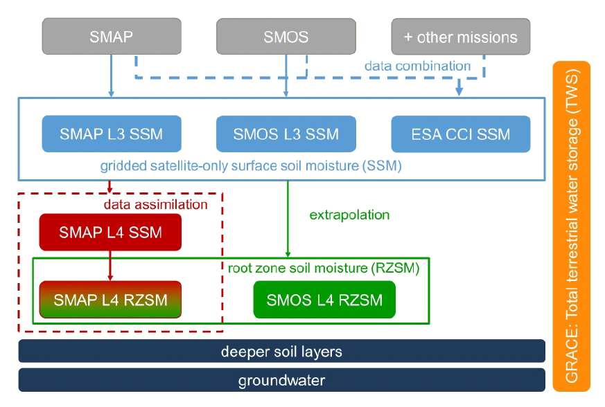
Given the potential value of combining SM and TWS observations for understanding water cycle dynamics as outlined above, the aim of this study is to investigate the global relationship between (1) non-standard daily TWS data from GRACE(-FO) and (2) several satellite SM products on different timescales to derive novel information content on Earth system dynamics. An overview of the data sets and their characteristics is shown in Fig. 1. The six SM products analyzed in this study can be categorized based on their degree of post-processing and their integration depth into the soil. Original Level 3 (L3) surface SM data sets of SMAP (Entekhabi et al., 2010) and SMOS (Kerr et al., 2010) are compared to post-processed Level 4 (L4) data products (SSM and RZSM) and a multi-satellite product provided by the European Space Agency Climate Change Initiative (ESA CCI; Gruber et al., 2019; Dorigo et al., 2017). While strong correlations of the two data types in the dominant seasonal cycle are to be expected, finding such correlations on shorter (down to sub-monthly and daily) timescales would be first-time evidence that satellite gravimetry can indeed observe such fast-changing SM signals, opening new opportunities of applications of this observation technology.
The paper is organized as follows: in Sect. 2, we describe the satellite data products used for the comparison of the different data sets (SM and TWS), followed by information on the applied data processing in Sect. 3. The results are presented in Sect. 4, first for the full signal and afterwards for sub-monthly timescales isolated by high-pass filtering. In both cases, we first illustrate signal characteristics using an exemplary time series for a specific grid cell, followed by global maps of correlation coefficients and relative time shifts to show the (dis)agreement between the data types.
2.1 GRACE and GRACE-FO data
To investigate fast temporal water storage changes, we use the daily gravity field solutions of the ITSG-Grace2018 model (Kvas et al., 2019) converted to a global time series of daily TWS anomalies. Compared to the standard monthly solutions, the limited satellite ground track coverage during 1 d does not allow for a stable global gravity field inversion; thus, additional information has to be introduced. The processing of the daily solutions is therefore carried out using a Kalman smoothing approach (similar to Kurtenbach et al., 2012), which introduces statistical information on the expected evolution of the gravity field over time in its process model. As a tradeoff, the resulting daily gravity field data are not fully independent daily solutions but exhibit some degree of correlation with previous time steps.
Daily gravity field data are given in the form of spherical harmonic coefficients (so-called Level 2 products) of the gravitational potential up to a degree of n=40, corresponding to a spatial resolution of 500 km. During the data processing, temporally high-frequency mass variations caused by tides (ocean, Earth, and pole tides), in addition to non-tidal atmospheric and ocean mass variations, are removed by subtracting the output of the geophysical background models from the observations (dealiasing; Dobslaw et al., 2017). Post-processing steps account for the effect of geocenter motion (adding the degree 1 harmonic coefficients given by Sun et al., 2016, on the basis of Swenson et al., 2008), replace the c20 coefficient based on a time series from satellite laser ranging (Cheng and Ries, 2017), and subtract the influence of glacial isostatic adjustment (GIA), using the ICE6G-D model (Peltier et al., 2017). No extra spatial filtering is needed because the Kalman smoother effectively suppresses spatially correlated noise. After these processing steps, the resulting gravity field models are assumed to primarily contain water mass changes above and below the Earth's surface and can be converted to equivalent water heights on a global geographical grid of , according to the following:
where λ and ϑ symbolize the spherical coordinates, M and R are the mass and the radius of the Earth, ρw is the density of water , denote the load love numbers (Lambeck, 1988), cnm are the spherical harmonic coefficients of the gravitational potential, and Υ(λ,ϑ) are the surface spherical harmonic functions. The degree and order of the spherical harmonic functions are denoted by n and m. For a reasonable overlap with all satellite-based SM products, we used the time period from April 2015 to December 2021 for our study, excluding the time span between the end of the mission GRACE (August 2017) and the start of the successor mission GRACE-FO (July 2018). Even though the Kalman smoother output provides a continuous daily time series without data gaps for the mission time periods, all days with insufficient GRACE observations were excluded from our analysis (i.e., days with an observation count of less than 10 000 observations per day as given on the website of the ITSG-Grace2018 product). On these days, the daily solutions are mainly informed by the process model of the Kalman filter and thus tend towards an a priori mean trend and annual signal. Calculation of the GRACE TWS data was done using the Gravity Recovery Object Oriented Programming System (GROOPS; Mayer-Gürr et al., 2021).
Limitations of the GRACE TWS data that are relevant for this study relate to the limited spatial resolution (i.e., 500 km for daily data, as stated above), which results in the TWS grid cell values not being independent from neighboring grid cells. This can lead to leakage effects (Longuevergne et al., 2013) of spatially localized mass variations that are small in their spatial extent but strong in magnitude, such as surface water storage change in lakes or reservoirs. Coastal areas should also be regarded with care because the limited spatial resolution prevents a strict separation between land and ocean signals in the GRACE data sets. While a mere dampening of the continental signal caused by a much lower mass variability on the ocean does not influence the correlations between the TWS and SM discussed in the present study, the so-called “leakage in” (Baur et al., 2009; i.e., spurious high-frequency ocean signal being leaked onto land areas) might have an influence on the comparison of TWS and SM in coastal areas. A more detailed discussion on this and a map (with areas that should be regarded with caution) is shown in Eicker et al. (2020, see Fig. 4 in their Supplement). Another issue that needs to be kept in mind when comparing TWS with SM data is the fact that the GRACE TWS observations represent the fully integrated vertical water column, which includes SM but is not limited to it. On the one hand, this is a challenge, as the two quantities (TWS and SM) are not directly comparable. One the other hand, it is the particular strength of the TWS observations to be sensitive to water storage dynamics that otherwise are not observable by remote sensing, such as those in deep soil layers down to the groundwater. To explore what we might learn from such differences (TWS versus SM), regarding hydrological process dynamics in the subsurface, is one motivation for this study.
2.2 Soil moisture data sets
Active or passive microwave remote sensing can observe SM in the top few centimeters of the soil, exploiting the fact that the dielectric constant of the soil changes with varying soil water content. Several dedicated instruments are currently in operation on different satellite missions. Active microwave sensors (radars) transmit an electromagnetic pulse to the Earth and measure the pulse's backscattered energy from the surface of the Earth, whereas passive microwave sensors (radiometers) observe the radiation naturally emitted by the Earth's soil, which is expressed as the brightness temperature (Robinson et al., 2008). The observed parameters (backscattered energy and brightness temperature) of both techniques depend on the dielectric constant of the soil, which allows the measurement of SM.
In our study, we use satellite-derived SSM products from the missions SMOS, SMAP, and from the combination data product ESA CCI, as well as RZSM products from SMOS and SMAP. Both SMOS and SMAP provide so-called Level 3 (L3) and Level 4 (L4) data, with L3 referring to the original satellite observations acquired over a 24 h period given as a multi-orbit global map of retrieved soil moisture (L3 data do not have complete global coverage), while L4 relates to post-processed data products. The way of post-processing differs between the two satellite missions and will be detailed below. The overlapping time span of all missions between April 2015 (start of the SMAP mission) and December 2021 was selected. In addition, it should be mentioned that the orbit direction (ascending/descending orbit) differs across the L3 products and therefore also the overpass time. In this study, the early morning overpass is chosen for the L3 satellite SM products. This is suggested for passive measurement methods, as the temperature difference between the soil surface and the vegetation canopy in the morning and night, in addition to the thermal difference between various types of land cover, within a pixel is reduced; this results in a minimization of SM retrieval errors and better reliability (Owe et al., 2008; Entekhabi et al., 2014; Lei et al., 2015; Montzka et al., 2017).
2.2.1 SMOS
The Soil Moisture and Ocean Salinity (SMOS; Kerr et al., 2010) satellite was implemented by ESA as part of the Earth Explorer missions and launched in November 2009. The satellite operates in a sun-synchronous orbit, and the ascending orbit overpasses the Equator at 6:00 local time. SM is observed by using an L-band radiometer, which receives the radiation emitted by the Earth's surface and measures the brightness temperature. This technique allows observations in the first few centimeters of soil (SSM). SMOS needs less than 3 d to revisit the same area, with a maximum spatial resolution of around 40–50 km.
In this study, we use the daily L3 (v3.0) SSM product of the Centre Aval de Traitement des Données SMOS (CATDS), operated by the Centre National d'Etudes Spatiales (CNES). The L3 data contain all of the collected SM data for each day on a global grid, with a spatial resolution of 25 km × 25 km (Al Bitar et al., 2017). Additionally, the CATDS L4 RZSM product is used, which propagates the L3 SSM data set (0–5 cm) into the underlying soil (5–40 cm), using an exponential filter. Then, from the 40 cm layer to the root zone layer (up to 1 m soil depth), a budget model based on a linearized Richards equation formulation is adopted to compute the water content (Al Bitar et al., 2013). The RZSM is a weighted average of the two layers (expressed in m3 m−3). Starting in February 2020, the SMOS L4 data set has been processed using a new algorithm. The method uses the SSM product from SMOS to calculate the SM of the root zone (1 m depth), based on a modified formulation of a recursive exponential filter, while considering soil properties and an optional implementation of transpiration (Al Bitar and Mahmoodi, 2020). As the data from 2015 to 2020 have not yet been reprocessed using the new algorithm, we decided to concatenate the two time series in order to adhere to the general comparison period of April 2015 to December 2021. An offset between the two differently processed time spans was calculated from the 14 d overlap period from 31 January to 13 February 2020 and removed from the February 2020 to December 2021 data to achieve a seamless transition with the previous data (April 2015 to January 2020). The L4 RZSM data set is provided in a global grid, with a spatial resolution of 25 km × 25 km.
2.2.2 SMAP
The Soil Moisture Active Passive (SMAP; Entekhabi et al., 2010) satellite was launched in January 2015 by the National Aeronautics and Space Administration (NASA) to observe SSM with an L-band active radar and passive radiometer. After a few months, the active system failed and since then only the passive system has been operational; it observes the brightness temperature of the Earth. Like the SMOS satellite, SMAP operates in a sun-synchronous orbit, but in contrast to SMOS, the overpass of the Equator at 06:00 local time occurs on the descending orbit. SMAP needs a maximum of 3 d to revisit the same area and measures the brightness temperature with a spatial resolution of around 40 km.
In this study, the L3 and L4 products from SMAP are used. The daily L3 data (v8.0; O'Neill et al., 2021) contain all SSM retrievals for an entire day mapped to a global grid with a spatial resolution of 36 km. In contrast, the L4 products are derived by assimilating SMAP surface brightness temperature observations into the Goddard Earth Observing Model System version 5 (GEOS-5) catchment land surface model. The land surface model is driven by observation-based surface meteorological forcing data, including precipitation, and represents essential land surface processes, such as the vertical movement of water in the soil between the surface and the root zone. Therefore, it should be pointed out that the resulting L4 data products cannot be regarded as purely being based on satellite soil moisture observations but have to be interpreted as a modeled data set that is heavily influenced by data assimilation and thus by the climate data used as input for the land surface model and by its model structure. Finally, the assimilation system interpolates and extrapolates SMAP observations in time and space using the land model, which gives estimates for the SSM (5 cm depth) and the RZSM (up to 1 m depth), which is provided with a temporal resolution of 3 h and a 9 km spatial resolution. Both L4 data sets (SSM and RZSM v6.0; Reichle et al., 2021), available from the website of the National Snow and Ice Data Center (NSIDC), are used in our analysis. To evaluate all products at the same daily scale, the SMAP L4 products are resampled to daily data by taking the average of all observations for 1 d (eight observations per day for a 3 h temporal resolution).
2.2.3 ESA CCI
The ESA CCI SM data set (Gruber et al., 2019; Dorigo et al., 2017) is provided as part of ESA's Climate Change Initiative (CCI). The ESA CCI SM product is based on harmonizing and merging SM retrievals from multiple satellites into a combined daily product. Three different data sets are provided, namely an active-microwave-only-based product, a passive-microwave-only-based product and a combined active and passive SM product.
We select the combined active and passive SSM product (v7.1) for our analysis. It provides daily SM observations, with a spatial resolution of 0.25∘ and is available from the ESA data archive. This product includes SM retrievals from active satellites, such as the Active Microwave Instrument Wind Scatterometer (AMI-WS) European Remote Sensing satellites ERS 1 and ERS 2 Wind Scatterometer Mode (SCAT) and MetOp-A and MetOp-B Advanced Scatterometer (ASCAT), and from passive satellites, such as the Nimbus-7 Scanning Multichannel Microwave Radiometer (SMMR), Defense Meteorological Satellite Program (DMSP) Special Sensor Microwave/Imager (SSM/I), the Tropical Rainfall Measuring Mission's (TRMM) Microwave Imager (TMI), Aqua Advanced Microwave Scanning Radiometer for Earth Observation Satellite (AMSR-E), Coriolis/WindSat, SMOS, GCOM AMSR2, and SMAP. Overall, this product covers SM data from 1978 to the present. It should be noted that tropical rainforest areas are completely masked out because of the strong signal scattering in the microwave observations caused by vegetation (Ulaby and Long, 2014).
A comparison between satellite gravimetry and the SM products is carried out on grid cell level; therefore, the SM products are harmonized to the same geographical grid used in Eq. (1) to compute TWS from the GRACE and GRACE-FO data. Downsampling was performed using a first-order conservative remapping function, which leads to a lower spatial resolution for the various SM data sets. Despite a remaining difference in the spatial signal content between the frequency-limited TWS and the gridded SM data, no further downsampling was performed in order to preserve the characteristics of the SM time series.
The linear trend of the time series is removed before examining the agreement between SM and TWS. To isolate sub-monthly variations, a third-order Butterworth high-pass filter with a cutoff frequency of 30 d is applied in the forward and backward directions (to avoid a phase shift). This filter conserves the phase but removes signals with periods longer than 30 d which dominate the time series. The computation of the high-pass filtered signal is presented in further detail in Appendix B.
Since a direct comparison of the absolute values of SM and TWS is not possible due to the different integration depths and units of the respective data sets, we analyze their relationship using Pearson’s pairwise correlation coefficient ρxy. Possible time lags between TWS and SM are determined using a cross-correlation analysis, which indicates the time shift for which two signals best agree with each other. Appendix A1 provides further information on these metrics. The data gaps in the TWS data set (see Sect. 2.1) were also excluded from the SM time series prior to comparison. No further temporal masking, e.g., based on quality flags, was performed for the SM data.
3.1 Spatial mask
The type of land cover can lead to limitations for observing SM. In densely vegetated areas such as tropical rainforests, the observed emissivity by passive satellites or the backscattered energy by active satellites is primarily caused by the vegetation (Ulaby and Long, 2014; Owe et al., 2001). In deserts, the SM signal may be unreliable, as the variability in the water in the upper soil is low (Dorigo et al., 2010). The problem of reduced sensitivity in deserts also accounts for the satellite gravimetry observations from GRACE and GRACE-FO, as their signal-to-noise ratio is low, and the noise floor of GRACE strongly dominates the time series. Other surface characteristics that limit the measurements of satellite SM are snow cover and frozen soil, since the dielectric constant of snow and frozen water varies significantly from the one of liquid water (Wagner, 1998).
Therefore, three spatial masks have been defined to identify problematic regions for observing SM. These are dense vegetation, regions with snow and frozen ground throughout large parts of the year, and areas with low SM (e.g., deserts), as seen in Fig. 2. To indicate dense vegetation, in our study we use the tropical rainforest mask that is also applied in the ESA CCI data set. Also, for regions with a large fraction of snow cover and frozen soil, the same method used for the ESA CCI mask is applied. It uses soil temperature (TS) and snow water equivalent (SWE) estimates from the Global Land Data Assimilation System Noah (GLDAS Noah) to flag satellite observations that were taken under the conditions of frozen soil (TS < 0 ∘C) and snow cover (SWE > 0 mm; Gruber et al., 2019). Grid cells in which more than 40 % of all observations are influenced by these conditions were included in the mask. We classify dry (desert) regions based on the SM signal variability, i.e., the root mean square (rms) of the daily SM time series in each grid cell. As a threshold value for low variability, we use twice the mean rms of a test region in the Sahara desert, where no major day-to-day SM variations can be expected. To define the mask with this criterion, we used the SMOS L3 data product. Using the other SM data products led to very similar results. In some regions, the low SM variability mask overlaps with the snow cover and frozen ground mask. The low SM variability areas are excluded from further analyses because no discernible signals of both SM and TWS can be expected. As we want to use the maximum of the available information of both data sets for the first analysis of this kind performed in the present study, values in the region of the other two masks (dense vegetation and snow cover and frozen ground) are considered in the analyses but will be discussed with care to recognize the limitations of SM retrieval.
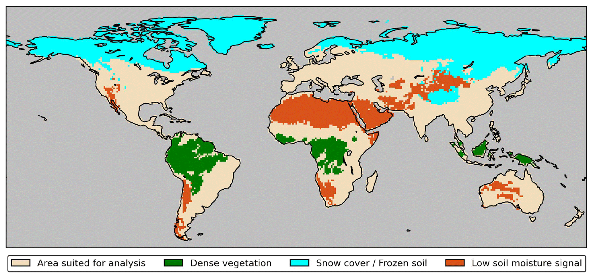
Figure 2Spatial masks applied in this study for low SM variability (red), dense vegetation (green), and snow cover and frozen ground (blue). In the other areas (beige; here denoted as the area suited for analysis), reasonable satellite-based SM signals can be expected.
4.1 Time series comparison for an example location
The comparison of time series between TWS from ITSG-Grace2018 and SM from various products is first shown for one exemplary grid cell. We chose one cell, with marked short-term and seasonal SM variations, close to the city of Kota (25∘ N, 75∘ E), located in the southeast of the Indian state of Rajasthan and characterized by a hot semi-arid climate, with a monsoon season from July to September. The location of this grid cell is indicated in the maps in Fig. 4 (blue circle). Figure 3 (top) shows daily TWS in this grid cell in comparison to SSM derived from satellite observations only. While TWS exhibits a comparatively smooth behavior for short timescales and a dominant seasonal signal, the SSM time series are of considerably higher variability at short timescales. One reason is the noise of the satellite SM observations themselves (e.g., Karthikeyan et al., 2017). On the other hand, this variability can partly represent a real signal, as near-surface SM exhibits quick wetting and drying dynamics from individual precipitation events and from subsequent evaporation. In contrast, the much larger integration depth of the GRACE observations down to groundwater results in integral water storage with much slower dynamics. Furthermore, it has to be noted that, for an integration depth of the SSM products of a few centimeters, the overall amplitudes of SM experience a change of the order of 40 vol. % (shown in Fig. 3) that corresponds to water storage changes that are 1 order of magnitude smaller than those of the GRACE-based TWS. An investigation into whether the fast-changing surface signals can also be detected in the GRACE data will be pursued in Sect. 4.3 for high-pass filtered time series. Comparing the time series of the three SSM products for this particular location, SMAP L3 and the multi-satellite combination product ESA CCI time series appear less noisy than the SMOS L3 time series, which is in good agreement with findings of, e.g., Montzka et al. (2017), Cui et al. (2017), Xu and Frey (2021), and Kim et al. (2021).
While there is a general correspondence in the dynamics of TWS and SSM regarding the dominating seasonal signal (strong rise in water storage and SM during the monsoon season followed by a quick decline), a time shift can be identified between both quantities. The seasonal maxima and minima of the GRACE time series occur approximately 1–2 months later than those of SSM. This can again be attributed to the slower and delayed water storage change in the deeper layers seen by GRACE, in which a change from dry to wet conditions (or vice versa) takes much longer to evolve than in the layers close to the surface. In addition to the main seasonal maximum, a minor secondary maximum can be identified each year in the period from November to January in the SSM time series, and it is particularly well visible in the SMAP L3 data (yellow line). For the TWS data, minor peaks or a less steep TWS recession can be observed during this period, although a more general statement is hindered by the gaps in the TWS time series. Further discussion on this feature follows in the next paragraph.
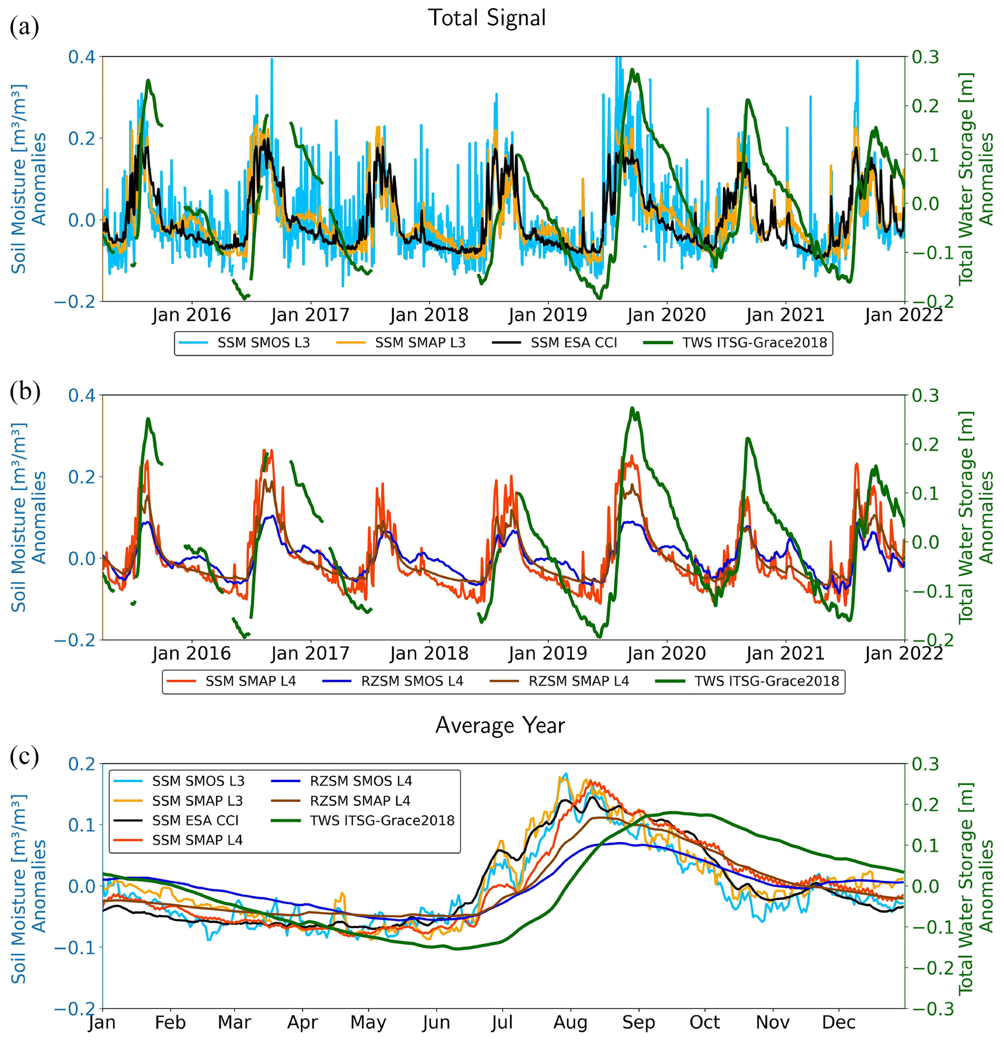
Figure 3Time series of TWS from ITSG-Grace2018 and satellite SM for an exemplary grid cell around Kota, Rajasthan, in India (25∘ N, 75∘ E). Linear trend components have been subtracted from all time series. (a) TWS ITSG-Grace2018 vs. SSM from SMOS L3, SMAP L3, and ESA CCI. (b) TWS ITSG-Grace2018 vs. SSM from SMAP L4 and RZSM from SMOS L4 and SMAP L4. (c) Time series of the average year between TWS and all SM products.
Figure 3 (middle) compares the TWS time series and the L4 SM products. For SMAP, both the surface (SSM) and the root zone (RZSM) products are the result of the data assimilation procedure described in Sect. 2.2.2. The SMAP L4 RZSM time series has a smaller variability compared to the SSM data at both short-term and at seasonal timescales. This is also the case for the L4 RZSM product of SMOS, in which the seasonal variability is dampened even more strongly. The secondary maximum in November–January obvious in the L3 products is still visible in the L4 RZSM data set of SMOS, since the physical extrapolation of the SSM data into deeper layers is applied for the SMOS L4 product. In contrast, the assimilation applied to SMAP L4 removes this second seasonal maximum for both the SSM and the RZSM data sets. This indicates that the signal seen in the direct satellite SM data is not represented by the forcing data of the underlying model (i.e., precipitation) and thus fades out in the L4 SMAP product. This shows how strongly SMAP L4 is influenced by the underlying model and the climate data used as model forcing. The secondary SM peak might thus be caused by extensive irrigation after the end of the monsoon season. The results corroborate a possible deficiency of the SMAP L4 product (i.e., that it is mainly driven by precipitation input in the data assimilation framework and thus does not represent the impact of irrigation). The combination of (near-surface) soil moisture products and TWS observations may thus shed light on how human activities and irrigation practices in particular translate into water storage changes in deeper soil zones. While the focus of this study is on shorter-term storage changes, overlapping trend signals in the unsaturated zone and in the groundwater that may be caused by these activities may be difficult to disentangle. However, a detailed analysis of this particular phenomenon is beyond the scope of this study.
The described characteristics of the different products are also confirmed when investigating the average year (i.e., the mean value for each day of the year shown in Fig. 3 at the bottom). Even though the short overlapping time span does not allow for the computation of a stable climatology, the increase in the seasonal signal with SM during the monsoon phase between July and September can clearly be identified. The SSM products exhibit a larger seasonal amplitude than the dampened RZSM counterparts. Furthermore, the time shift between SSM and TWS is generally larger than for the RZSM products. Here it can be concluded that the dynamics of RZSM are closer to the variability in the integral TWS signal that represents the entire water column, even though the RZSM data still miss the even slower processes in deeper soil layers and in groundwater.
4.2 Global analysis
The correspondence of the daily time series of TWS from ITSG-Grace2018 with the various SM products is analyzed globally for each 1∘ continental grid cell and displayed as global maps of the correlation coefficient in Fig. 4. Desert areas, according to the definition provided in Sect. 3.1, are excluded, as the GRACE signal is dominated by noise in these regions, and no reasonable comparison is possible. Additionally, Fig. 5 shows the cumulative distribution functions (CDFs) of cell-based correlation values, both globally and separately, for the major land cover types shown in Fig. 2.
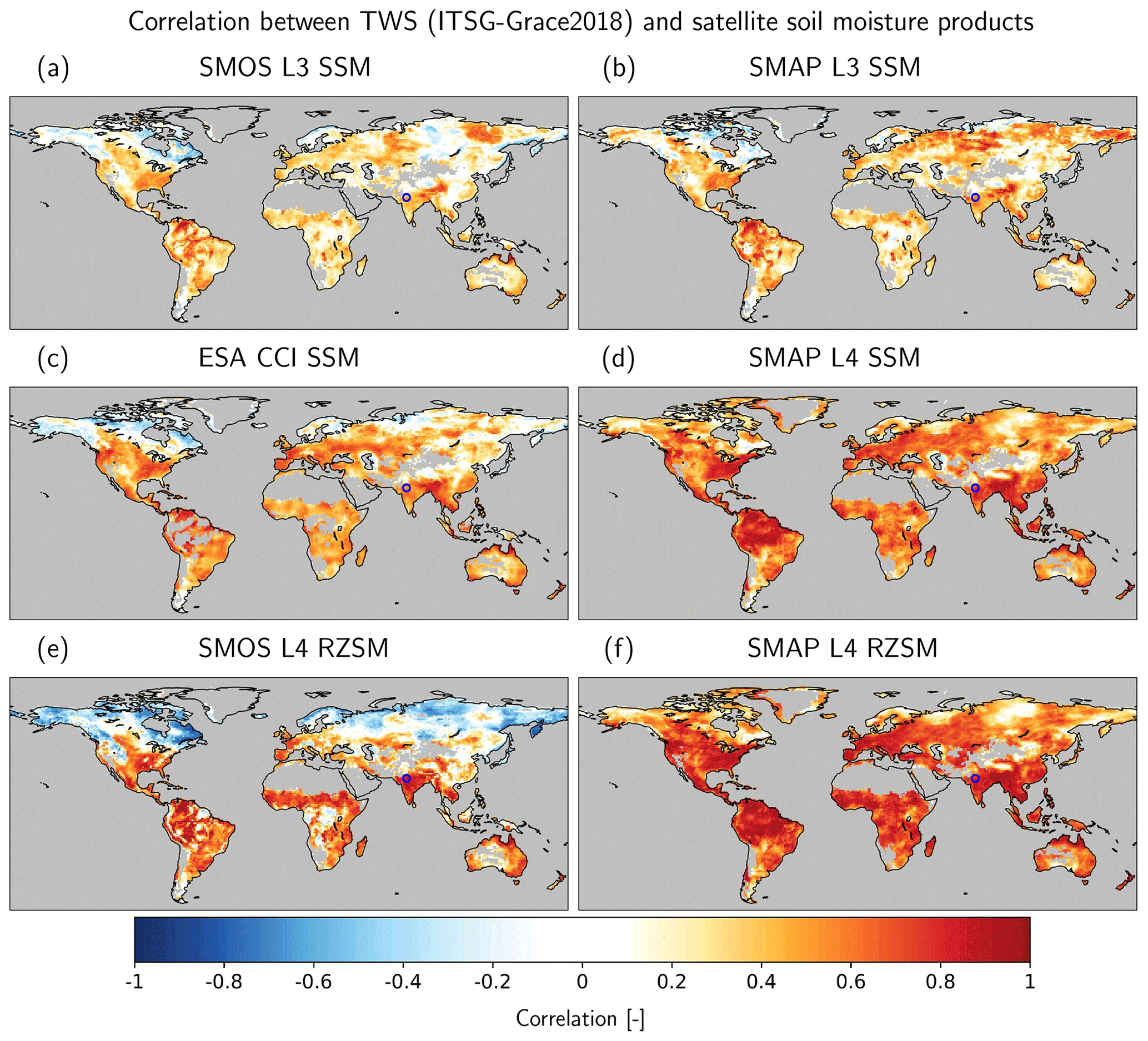
Figure 4Comparison of the correlation coefficient between all SM products and ITSG-Grace2018. Desert regions are masked out due to low water variability. In all maps, the location of the exemplary time series in India (see Fig. 3) is marked with a blue circle.
The global patterns of regions with comparably large correlations between GRACE TWS and SM are similar for all SM products. These regions are particularly found in humid climate zones and in seasonally dry climates (parts of tropical South America, Southeast Asia, southeastern USA, northern Australia, and the outer tropics in Africa). The absolute correlation values differ markedly between the SM products. The smallest correlations are found for the satellite-only L3 SSM data products (Fig. 4a–c). While maximum values in individual grid cells can reach up to 0.92 (SMOS) and 0.93 (SMAP), the median values amount to 0.23 (SMOS) and 0.27 (SMAP) only. SMOS L3 SSM has negative correlations (Fig. 5), particularly in the northern latitudes that are at least partly influenced by snow cover and frozen ground (Fig. 5c), and has fewer large positive correlations in grid cells that are potentially well suited for SM remote sensing (i.e., that are not influenced by snow, ice, or dense vegetation; Fig. 5b). The latter might be attributed to a larger noise level in the SMOS than in the SMAP time series. The combination data product ESA CCI (black curve in Fig. 5b) generally shows larger correlation values than both the single mission products (except in the northern latitudes), particularly in South America, Africa, and Australia (Fig. 4c). Please note that the masking of, e.g., rainforest areas in the CCI product leads to an overall smaller number of grid cells for the comparison than for SMOS or SMAP. The overall larger correlation of ESA CCI implies that the ensemble product weighs down the spurious contributions of individual data sets. Nevertheless, the interpretation needs to be done with caution, as TWS cannot be directly taken as a benchmark for SSM, and the limitations of the GRACE data product outlined in Sect. 2.1 might additionally hamper the comparison.
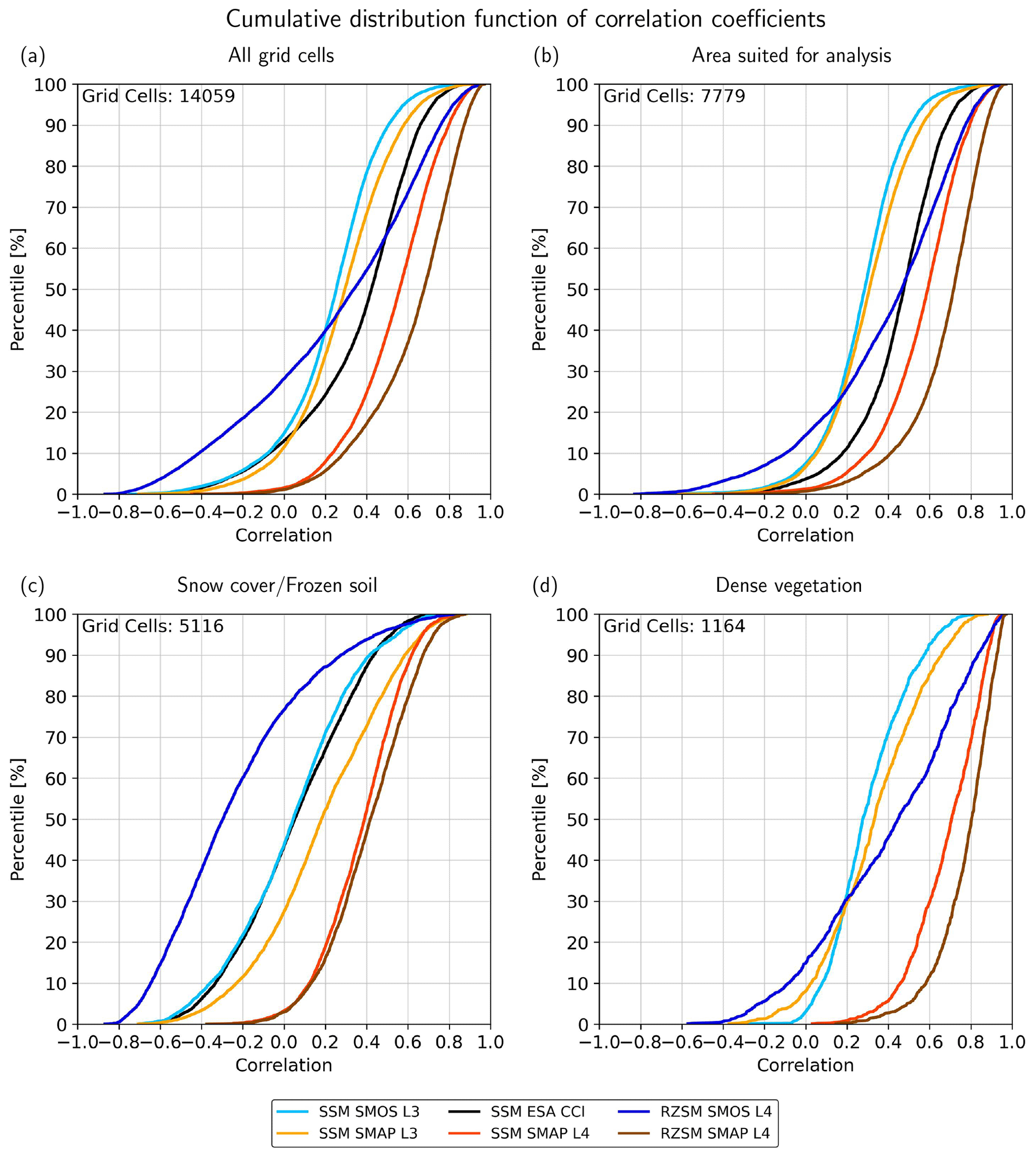
Figure 5Cumulative distribution functions (CDFs) of cell-based correlation values. (a) Showing the CDFs of all grid cells globally. (b, c, d) Showing the grid cells for the major land cover types, as defined in Fig. 2. In the upper left corner, the number of grid cells used for the creation of the individual CDFs is shown.
The effect of using a land surface model with data assimilation for generating the SMAP L4 SSM product is a strong increase in the correspondence of the temporal dynamics of this SM data set with GRACE-based TWS (Fig. 4d). The CDF in Fig. 5a (red line) reveals the most common correlation values in the range of 0.4–0.7, with a median of 0.52. This increase in the correlation for the L4 SSM data indicates that constraining the SM dynamics by a deterministic modeling approach and by independently observed forcing data, such as precipitation rates and air temperature, leads to a model-dominated product with considerably less noise than the L3 SSM product. For the L4 RZSM products of both SMOS and SMAP, their larger integration depth leads to another increase in the agreement with TWS compared to the respective surface products (Fig. 4e, f). This again indicates that reflecting the slower and delayed water transport processes in deeper soil layers in the L4 RZSM products causes their dynamics to be more similar to the integrative GRACE-based TWS, in particular with respect to the temporal phase (also see the time shift analysis below). This applies in particular to the grid cells that are reasonably suited for satellite-based SM monitoring for which the CDFs are shifted strongly to higher correlation values compared to the L3 data, with the most common values of around 0.7 (SMOS) and 0.8 (SMAP; Fig. 5b). In contrast, for SMOS L4 RZSM in high northern latitudes, correlations with TWS become even more negative than for SMOS L3 SSM (see the time shift analysis below). Xu et al. (2021a) have already shown that the SMAP L4 RZSM product outperforms the SMOS L4 product in terms of agreement with in situ measurements from the International Soil Moisture Network, particularly in the Northern Hemisphere.
The different integration volumes and the different processes acting on SM and TWS cause a time shift between their respective dynamics (e.g., Fig. 3). We use a cross-correlation analysis (see Appendix A1) for each grid cell to investigate the time shift on a global scale. Regarding the maps in Fig. 6, a negative time shift (blue colored grid cells) indicates a delay of the GRACE signal; i.e., the maximum of the dominant seasonal signal of TWS occurs later in the year than the maximum of SM. In the Arctic regions, mostly positive shifts (in some cases more than +120 d) are seen, in particular for the two SMOS products (see also the CDFs in Fig. 7). Snow accumulation leads to an increase and a maximum of TWS during the winter season, whereas the maximum of SM is reached during the melting season several months later, resulting in a delay of SM versus TWS. This effect becomes even more pronounced when the further delay by SM storage in deeper layers is considered in the L4 root zone products of SMAP and, in particular, SMOS. Negative correlation coefficients of TWS and SM time series are a consequence of the inverse seasonal dynamics of the two storage terms (Fig. 5). The least positive time shifts in the northern latitude regions are visible in the ESA CCI data set, which already masks out the data in the time series when observations were taken under the conditions of frozen soil and snow cover (see Sect. 3.1). Positive time shifts are also seen in some tropical forest regions (e.g., the Amazon and Congo rainforests), where the dense vegetation cover hampers the SM retrieval. This is particularly evident in the SSM L3 products (SMOS and SMAP) and persists in the SMOS RZSM, while the data assimilation introduced for SMOS L4 strongly reduces this effect. The positive time shifts can thus be attributed to artifacts in the SM data rather than to a hydrological signal.
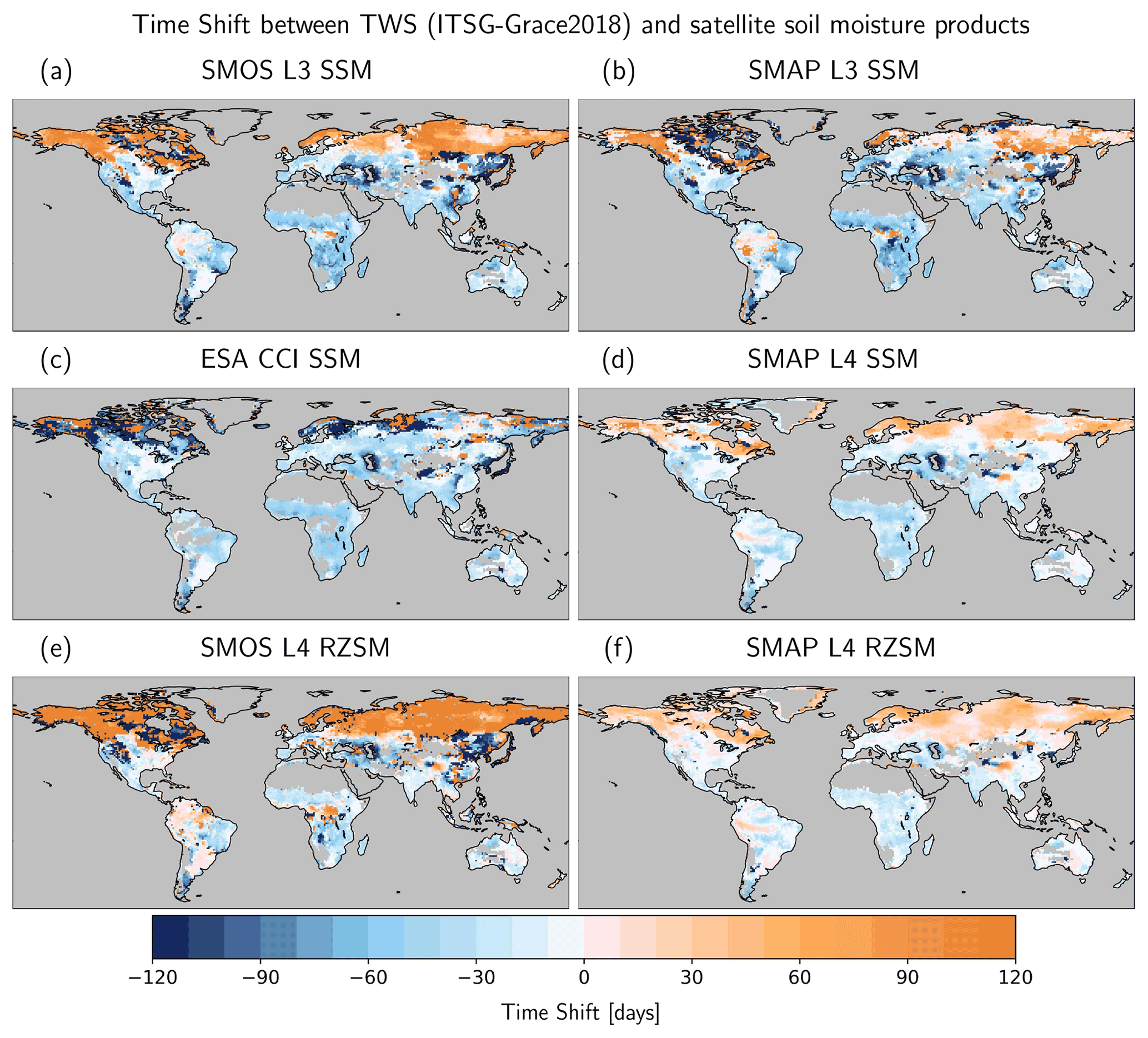
Figure 6Time shift between SM and TWS time series per grid cell. Negative numbers imply that TWS is delayed in comparison to SM.
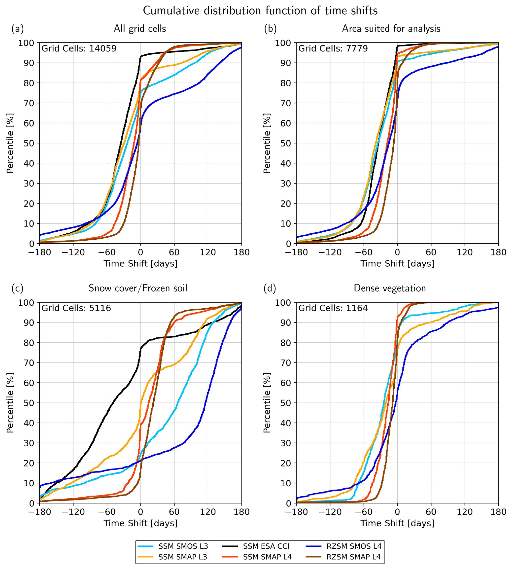
Figure 7Cumulative distribution functions (CDFs) of the cell-based time shift. (a) Showing the CDFs of all grid cells globally. (b, c, d) Showing the CDFs for grid cells for the major land cover types which are shown in Fig. 2. In the upper left corner, the number of grid cells used for the creation of the individual CDFs is shown.
In grid cells that are neither influenced by snow cover nor by dense vegetation (Fig. 7b), the time shifts are primarily negative, indicating the delayed dynamics of TWS compared to SM. For the majority of the products, the time shifts are negative and can reach up to −90 d and beyond. A comparison of the different products reveals that the time shifts decrease (i.e., become less negative) the closer the SM products conceptively resemble TWS. The three surface SM products from ESA CCI, SMAP L3, and SMOS L3 show the highest negative time shifts (up to −60 to −90 d in Fig. 6), with median values of −35 d (both ESA CCI and SMAP L3) and −32 d (SMOS L3). The time shifts are smaller for SMAP L4 (SSM; median of −17 d) and even smaller for the RZSM products, with median values of −5 d (SMAP L4 RZSM) and −13 d (SMOS L4 RZSM). This supports the assumption that adding the SM dynamics of deeper soil layers to SSM increases the resemblance to the integrated TWS signal. For SMOS L4 SM, the extrapolation into deeper soil layers even leads to a change from a negative time shift to a positive time shift (i.e., TWS dynamics preceding those of SMOS L4 RZSM) in 17 % of the land areas, e.g., in parts of South America, Asia, and Australia. This points out possible deficiencies in the depth-scaling algorithm for SMOS L4 in some regions in terms of the way that it represents the transport and storage processes from the surface to deeper soil layers with too many delays and that the rates of reduction in the water storage in the deeper layers by evapotranspiration and percolation and/or runoff may be underestimated, thus leaving too much water in the storage for a time period that is too long. While the limitations of the GRACE observations can also be expected to cause some discrepancy between the two data types, there is no known deficit in the GRACE data that may spuriously pull their dynamics to an earlier stage.
4.3 Sub-monthly variations (high-pass filtered data)
The exemplary comparison of the TWS and SM time series in Fig. 3 suggests that fast-changing SM signals might be masked in the TWS time series by the dominating slower dynamics of the deeper layers in the unsaturated zone and in groundwater. Therefore, we isolate the water storage changes on sub-monthly timescales by applying a high-pass filter (third-order Butterworth filter) with a 30 d cutoff frequency (see Appendix B for details). Exemplary high-pass filtered time series for 1.5 years of SMAP L4 RZSM and TWS from ITSG-Grace2018 are shown in Fig. 8 for the same grid cell as in Fig. 3. The overall correlation of the two time series amounts to ρ=0.33, but it varies strongly with signal strength. While the GRACE time series is dominated by noise and only a very small correlation to RZSM of ρ=0.17 was found in dry months (October to June) with very small high-frequency water storage fluctuations, the correlation is higher in the monsoon season (July to September) with ρ=0.45. Additional high-pass filtered time series for grid cells belonging to different climate zones are presented in Appendix C.
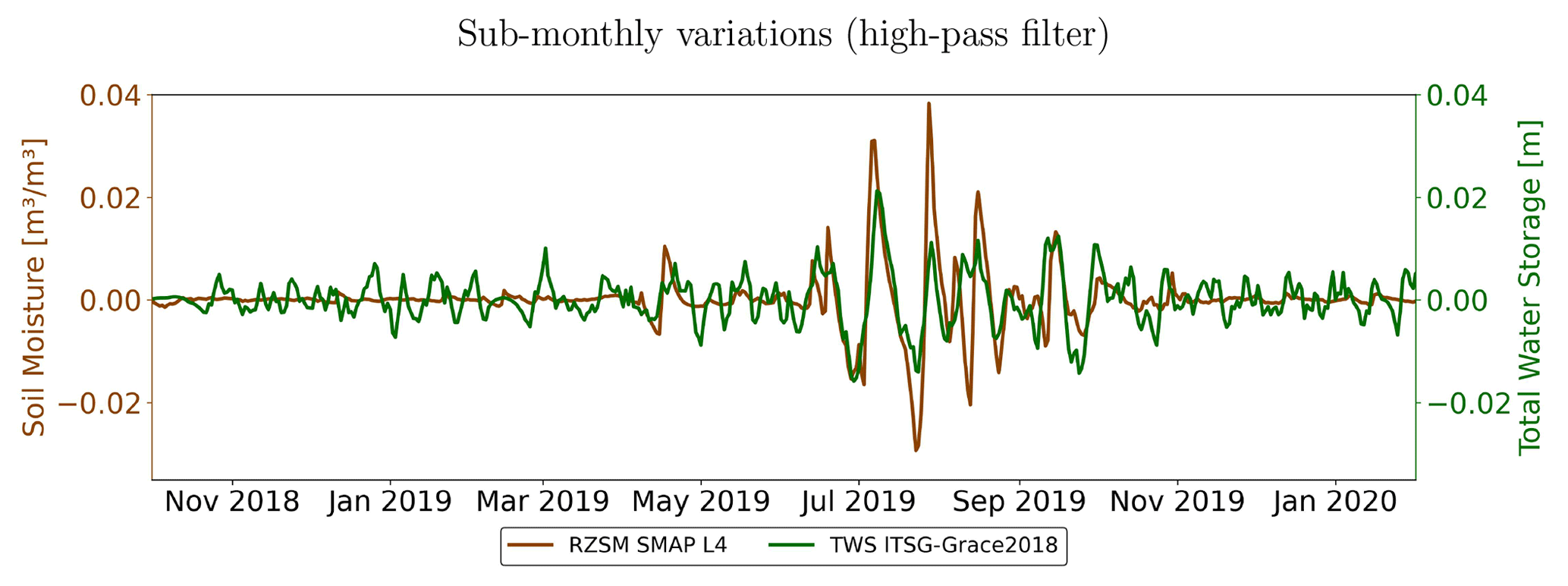
Figure 8High-pass filtered time series of TWS from ITSG-Grace2018 and RZSM from SMAP L4 for an exemplary grid cell in India (25∘ N, 75∘ E).
The correlations of the high-pass filtered TWS and SM time series (Fig. 9) are considerably smaller than those of the unfiltered time series. This can be expected, as the seasonal storage variations that often cause high correlation values for the unfiltered time series are not present anymore in the filtered ones. Nevertheless, correlations of the sub-monthly signals are generally positive, with only a few grid cells showing negative correlations. Non-significant correlations are stippled in Fig. 9 (for more information on significance testing, see Appendix A2). Again, it can be observed that RZSM products have a stronger correlation with TWS than their SSM counterparts. While the numbers are very small for the SSM of SMOS L3 (maximum value of ρmax=0.33 and significantly positive correlations in only 26 % of land areas covered by the data product, with desert areas excluded), they are larger for SMAP L3 SSM products (ρmax=0.37 and 43 % significantly positive). Again, the larger noise floor of the SMOS data set most likely dominates the high-pass filtered time series. The share of grid cells with significantly positive correlations increases for the combination data product ESA CCI (ρmax=0.38 and 58 % significantly positive) and even more for the data-assimilated product of SMAP L4 SSM (ρmax=0.40 and 71 % significantly positive). The former reveals the positive effect of combining several SSM data sets, which very likely results in a reduction in the high-frequency noise, and the latter indicates the influence of the forcing data of the underlying land surface model. In particular, it can be argued that model forcing with observation-based rainfall data causes major SSM increases to be closer in time and magnitude to the water storage increases that are seen by the GRACE observations. For the root zone, the percentage of the significantly positive grid cells is still low for SMOS L4 (37 %), with only a few larger areas in western Brazil, the south of Africa, and India, but the magnitude of the correlations has increased (ρmax=0.50). For SMAP L4 RZSM, the values are significantly positive in the largest parts of the continents (77 %), with exceptions only in the very high latitudes and some small spots in dry regions in Africa, Australia, and Asia. In large regions (particularly in the southeastern United States, large parts of South America's southeastern region, the Ganges–Brahmaputra basin and China, and northern Australia), the correlations are in the range of 0.5, reaching maximum values of ρmax=0.62. Overall, even though correlations are rather low for the high-pass filtered signals (with the exception of SMAP L4), they are significantly positive in large parts of the continents, hinting at the fact that satellite gravimetry and SM remote sensing are sensitive to the same hydrological dynamics, even for timescales shorter than 1 month.
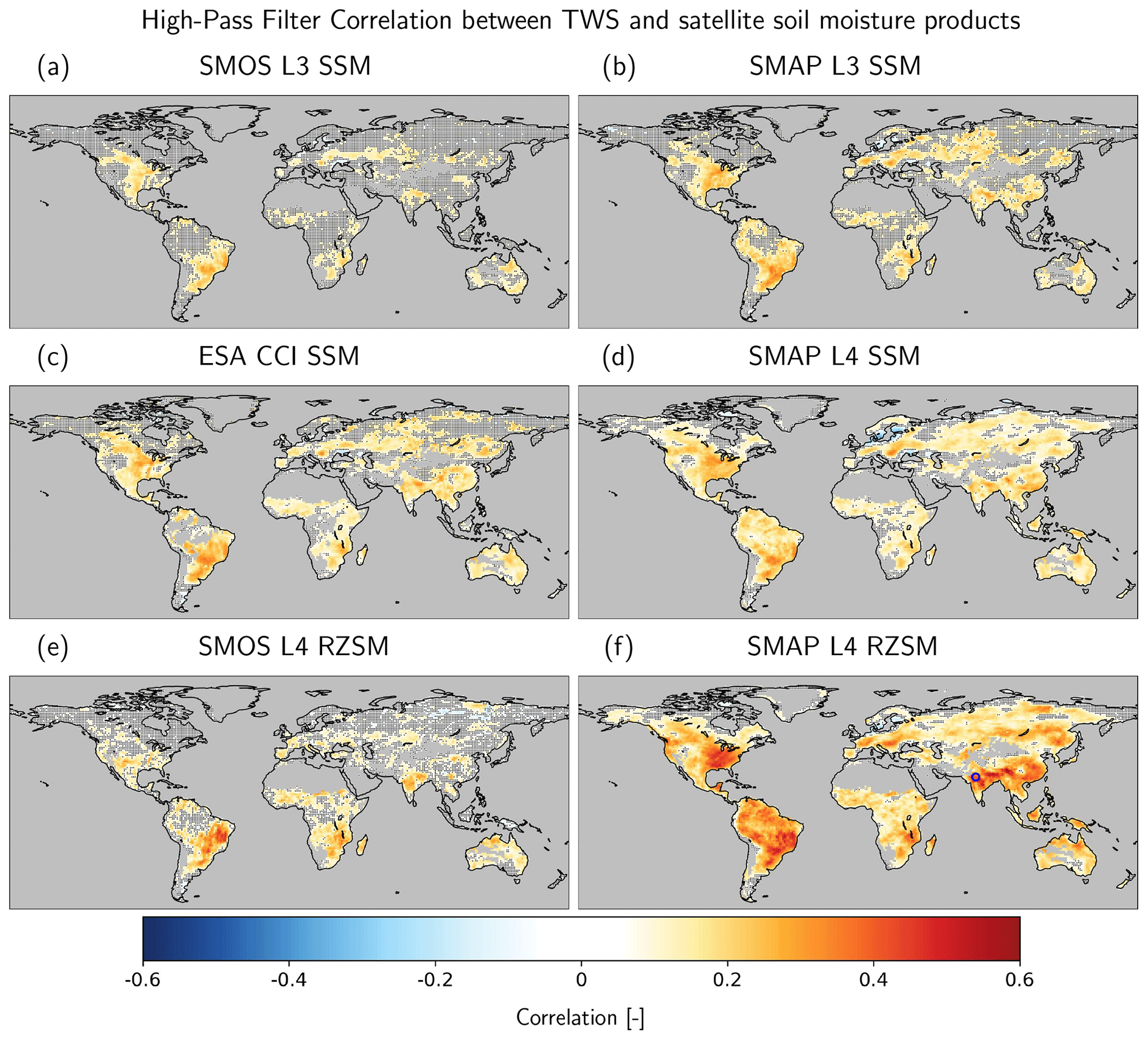
Figure 9Correlation coefficients of high-pass filtered SM and TWS time series. Grid cells with non-significant correlations are stippled. In the lower-right map (f), the location of the exemplary time series in India (see Fig. 8) is circled in blue.
Finally, by computing the cross-correlation function for the high-pass filtered signals, we determine, for each grid cell, the time shift in the TWS versus the SM time series that leads to the highest correlation (Fig. 10). Time shifts larger than ±15 d are masked out because they have no physical meaning, given that a high-pass filter of 30 d was used. The remaining regions with valid results noticeably overlap with the regions in which some correspondence of TWS and SM dynamics has already been found in the correlation analysis with an unshifted time series (Fig. 9). The time shifts found for the high-pass filtered time series are considerably smaller than those found for the full unfiltered signal. Time shifts tend to be negative, with up to −3 d for all SSM products (i.e., TWS is lagging behind SSM). For the RZSM products, however, the time shifts are less negative or close to zero (SMAP L4) or even positive (SMOS L4). The negative time shifts illustrate that GRACE observations represent the depth-integrated water storage dynamics in the subsurface that are delayed relative to SSM, even at sub-monthly timescales. This is corroborated by the observation that the time shifts mostly vanish when deeper layers are included in the SM product (SMAP L4; i.e., when the SM product becomes conceptually closer to the storage that is represented by the TWS observations). The positive time shifts for the SMOS L4 relative to TWS in most parts of the world indicate that the depth-scaling approach used for SMOS L4 may represent transport and storage processes from the surface to deeper soil layers with too much delay, which is similar to the results obtained with the full unfiltered signal. Even for the short timescales considered here with the high-pass filtered signal, some processes such as daily evapotranspiration or runoff that cause water to be removed from the storage may be underestimated.
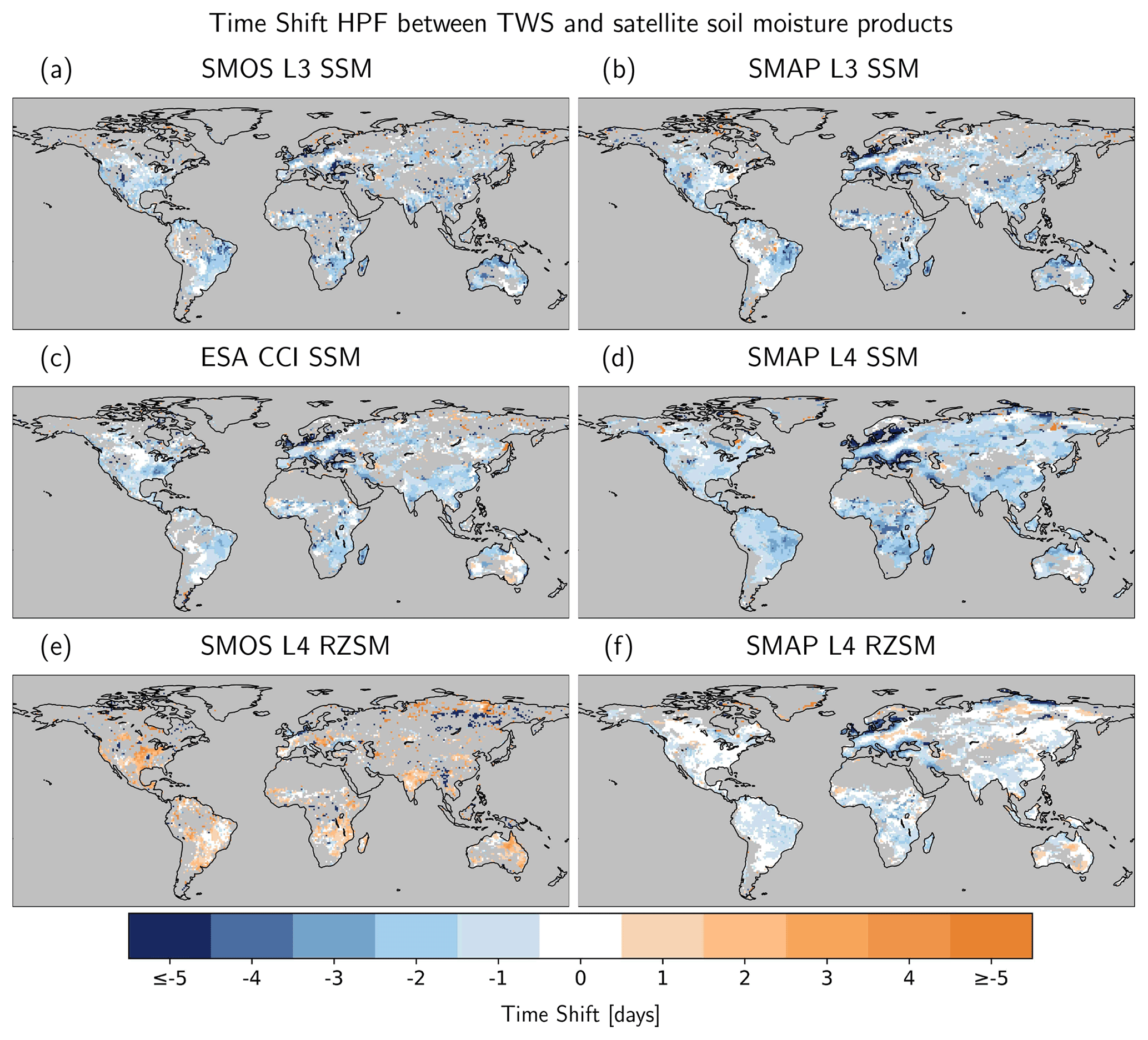
Figure 10Time shift between high-pass filtered soil moisture and total water storage time series per grid cell. Negative numbers imply that the TWS is delayed in comparison to the SM.
In this study, we investigated the global relationship of satellite-based SM products and non-standard daily water storage observations from the GRACE and GRACE-FO satellite gravimetry missions. The SM products differ with respect to satellite data (SMAP, SMOS, or a combination of various satellites), soil depth (surface SM or root zone SM), and the degree of post-processing (L3 or L4 data products). Comparisons were carried out by correlation analyses for both the full signal and for sub-monthly variations obtained via high-pass filtering the time series with a 30 d cutoff frequency. Strong correlations between TWS and the different SM products generally occur in the same regions. These regions are mainly characterized by a seasonally wet or semi-arid climate, such as the east and south of Africa, northern parts of India, east Australia, the southeast of China, Eastern Europe, the northwest and southeast of the United States, and significant parts of South America's southeastern region. For many regions, TWS dynamics are delayed relative to the SM dynamics for both short-term variations at the scale of few days and when considering the seasonal dynamics. In particular, in cold and snow-dominated regions, low correlations between TWS and SM dynamics prevail, and the seasonal TWS dynamics are ahead of the SM dynamics.
From a hydrological point of view, both quantities (SM and TWS) actually represent different quantities regarding their spatial domain (first centimeters of soil (SSM) vs. root zone (RZSM) vs. integrated water column of all storage compartments (TWS)), their units (volumetric percentage of water in the soil vs. water mass), and their spatial and temporal variability. The observed (dis)agreements of the SM and TWS time series and the time shifts between them therefore give insights into the relationships between the different water storage compartments, including moisture variations in different soil depths. It should be noted, though, that in some regions non-hydrological effects that remain in the GRACE data (e.g., major earthquakes) or storage variations in other terrestrial water storage compartments that have not explicitly been taken into account in the present study, in particular surface waterbodies, might affect these relationships. Due to the limited spatial resolution of GRACE (i.e., 500 km for the daily gravity field models use here), such strongly localizing effects might also hamper the comparison between SM and TWS in surrounding areas due to spatial leakage, as outlined in Sect. 2.1. While both SM and TWS products are sensitive to the effects of irrigation on near-surface soil moisture, GRACE-based TWS can provide additional information on the effect of such human impacts on water storage dynamics in the deeper unsaturated zone and in the groundwater, although the latter may be difficult to disentangle if it overlaps with groundwater withdrawal in the same region.
The fact that satellite gravimetry can detect high-frequency signals that are related to SM variations, at least in areas and time spans with sufficiently large short-term variability, is quite remarkable in itself and is shown for the first time in this study. While the standard products of the GRACE and GRACE-FO mission are monthly averages of water storage anomalies, the present study adds a new thematic field in which there is valuable information on the daily GRACE data that goes beyond earlier examples, e.g., floods or hydrometeorological fluxes (Gouweleeuw et al., 2018; Eicker et al., 2020).
For regions where SM plays a dominant role for TWS variations, the results indicate that satellite gravimetry can be used to identify the differences between SM products. Hydrological processes that are relevant for redistributing water vertically in the soil, particularly the percolation into deeper soil layers, can be identified as time shifts between the SM and TWS time series.
In this respect, our results give a preliminary indication that gravity-based TWS variations might have the potential to assess different methods of depth scaling (i.e., methods that are used to extrapolate surface SM variations to deeper soil layers). Such an assessment might be based on the analysis of time shifts between TWS and the depth-scaled SM time series. Assuming that the TWS signal for the region of interest and for the relevant temporal scale is dominated by SM variations, the absence of a time shift between TWS and the depth-scaled SM time series might be considered to be an indicator of a suitable depth-scaling approach. For the analyses presented here, this tends to be the case for the SMAP L4 RZSM data. In contrast, negative time shifts (i.e., SM dynamics that are ahead of those of TWS) may indicate that the delay of depth-integrated SM dynamics introduced by the depth-scaling approach is not sufficient enough. In turn, positive time shifts after depth scaling, as found here for some regions for the SMOS L4 RZSM data, may point out that the depth-scaling approach mimics the soil water redistribution processes in a way that causes a delay that is too large for the SM dynamics.
While satellite gravimetry can identify short-term SM changes in regions and time spans with large sub-seasonal storage variability, this does not work well in cases with low signal-to-noise ratios (SNRs) of high-frequency variations. In the current study, spatial masking was applied so that desert areas were completely excluded from the analysis, and some other regions (frozen ground and dense vegetation) were discussed separately from the areas that are not influenced by either effect. Nevertheless, there are still many areas worldwide where the SNR is high in certain periods, e.g., during the rain season but low in other time periods. Therefore, an additional temporal masking and the exploration of metadata such as snow flags or indicators of low SNR is promising for an extended comparison in future.
Ongoing improvements to the GRACE/-FO data processing and future improvements in gravity field determination with the GRACE-FO laser ranging instrument measurements and with next-generation gravity missions (NGGMs), such as a constellation of two GRACE-like missions operating simultaneously at differently inclined orbits (Purkhauser et al., 2020), will give prospective increases in the temporal and spatial resolution of satellite-based TWS data in future. This can be expected to be particularly beneficial for analyzing fast-changing and rather small-scale SM variations. The present study provides the first evidence of the insights into the hydrological dynamics that can be gained from a combination of TWS and SM remote sensing data.
A1 Correlation and cross-correlation
Suitable metrics are required to compare the time series of soil moisture (SM) and terrestrial water storage (TWS) for each continental grid cell. Since a direct comparison of the absolute values of the two variables is not possible due to the different integration depths and units, we analyze their relationship using Pearson’s pairwise correlation coefficient ρxy, which is defined as the covariance of two variables (x,y) divided by the product of their standard deviations:
The summation is performed over all daily time steps t of the available time series with a length of T days.
Possible time lags between the TWS and SM time series are determined using cross-correlation analysis, which identifies the time shift k for which the two time series show maximum correlation. The concept of cross-correlation is shown in Eqs. (A2) and (A3), according to Box et al. (1994), in which first the covariance cxy between the two time series xt and yt for a given time lag k is calculated as follows:
where and denote the mean values of the time series, and t indicates the respective point in time. We use n=180 in our analysis, resulting in a total of 360 different covariances for each grid cell ( to 180; ±6 months). From the covariance, the cross-correlation r is computed as follows:
where sx and sy denote the standard deviations of the time series. The time lag between SM and TWS is the value of k for which the maximum cross-correlations is obtained.
A2 Significance test
To identify grid cells with significant correlations between different time series, we use hypothesis testing, with the null hypothesis H0 stating that the correlation is not significantly different from zero and the alternative hypothesis HA assuming a non-zero correlation.
A statistical test is carried out by computing the test variable T, which is distributed with n−2 degrees of freedom, according to Student's t distribution.
In Eq. (A5), n is the total number of days with both TWS and SM observations for the respective grid cell. The test assumes uncorrelated observations from 1 d to the next, which, however, is not strictly the case for the time series at hand. An autocorrelation analysis was carried out for a large number of exemplary grid cells to determine a mean correlation length of 3 d for surface and 5 d for root zone products. Consequently, the degree of freedom was adjusted to (SSM) or (RZSM). For the significance test, we chose a significance level of α=0.05 and calculated the corresponding quantiles (SSM) or (RZSM). If T≤K, the null hypothesis cannot be rejected, and the correlation is assumed to be insignificant. If T>K, then it is reasonable to assume that the alternative hypothesis is correct and that the correlation deviates considerably from zero.
In this section, we demonstrate the computation of the high-pass filtered signals for the exemplary grid cell around Kota, India (also shown in Sect. 4.3 of the main text). Figure B1 shows the TWS from ITSG-Grace2018 (green lines) and RZSM from SMAP L4 (brown lines) over a 15-month period (October 2018 to December 2019). The Butterworth high-pass filter, with a cutoff frequency of 30 d, was applied to remove signals with periods longer than 30 d and thus to isolate sub-monthly fluctuations. The darker green and brown colors illustrate the high-pass filtered signal for both variables. Additionally, the corresponding low-pass filtered signals (i.e., containing signals with periods longer than 30 d) are added as dotted lines. Summing up the high-pass filtered signal and the low-pass filtered signal again results in the original full signal (shown in the respective brighter colors). It can clearly be seen that the high-pass filtered time series capture the fast variations present in the original time series. These time series are the same as those displayed in Fig. 8.
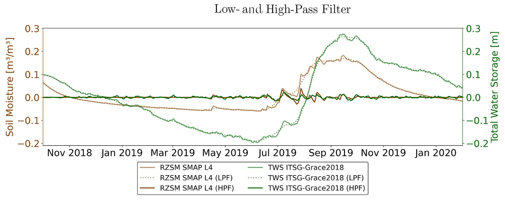
Figure B1Sub-monthly signals using a Butterworth high-pass filter (HPF), together with the full and the low-pass filtered (LPF) time series, which are shown here for TWS from GRACE and root zone soil moisture (RZSM) from SMAP.
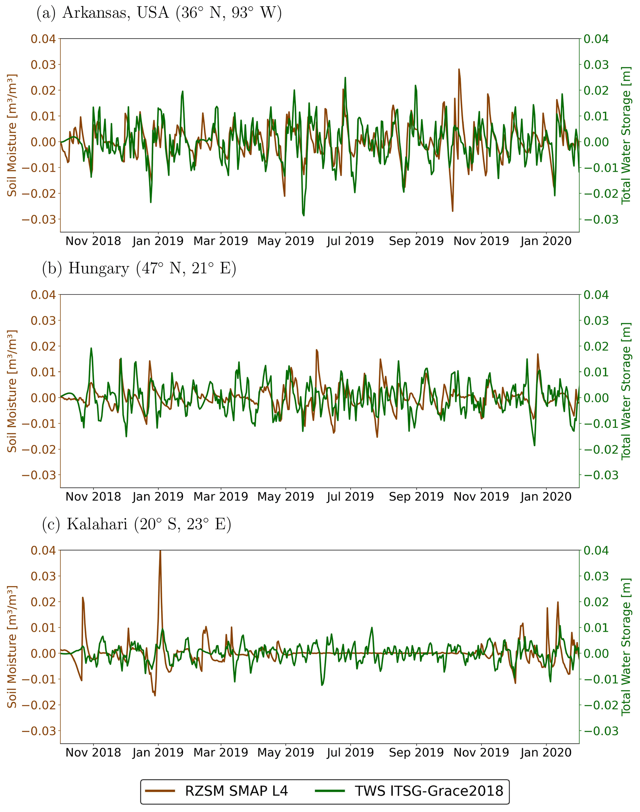
In addition to the high-pass filtered signal computed for the example grid cell in Kota, India, as shown before, Fig. C1 displays the high-pass filtered signals for SM from SMAP L4 RZSM and TWS from ITSG-Grace2018 in some other geographical locations of different aridity. These places were chosen to illustrate the dynamics of the two variables under different environmental conditions and signal characteristics. Figure C1a is for a location in the northwest of the state of Arkansas in the United States. The climate is humid and sub-tropical, with a hot summer and no specific dry season. Accordingly, the time series show fast fluctuations and a high correspondence of SM and TWS throughout the year, with a correlation of ρ=0.43. At a location in Hungary (Fig. C1b), with a humid and continental climate with warm summers, rain occurs throughout the year, while snow occurs during the winter months. The high-pass filtered SM and TWS time series show a correlation of ρ=0.31 at this location. The time series of Fig. C1c are for a location north of the Kalahari Desert in Botswana. The climate there is semi-arid and mostly dry throughout the year, but there is a wet period, with strong rainfall events during the summer. These events are clearly visible in both TWS and SM time series, with good correspondence, while no correlation and largely noise in the TWS data are visible during the dry period. At this location, the correlation over the entire time period is low, with ρ=0.11, but it is higher when only the precipitation period is considered, with ρ=0.23.
The daily GRACE data products of ITSG-Grace2018 are publicly available from TU Graz (https://doi.org/10.5880/ICGEM.2018.003, Mayer-Gürr et al., 2018). The ESA CCI soil moisture product can be downloaded from the ESA’s Climate Change Initiative (CCI) web page (https://doi.org/10.5285/ea3eb0714dc6402b905fe9f7ee50dbbc, Dorigo et al., 2023). Soil moisture products (Level 3 and Level 4) from the ESA’s SMOS mission are made available by the Centre Aval de Traitement des Données SMOS (CATDS; https://doi.org/10.12770/9cef422f-ed3f-4090-9556-b2e895ba2ca8, CATDS, 2022a; https://doi.org/10.12770/316e77af-cb72-4312-96a3-3011cc5068d4, CATDS, 2022b). Soil moisture products (Level 3 and Level 4) from NASA’s SMAP mission are provided by the National Snow and Ice Data Center (NSIDC; https://doi.org/10.5067/OMHVSRGFX38O, O'Neill et al., 2021; https://doi.org/10.5067/08S1A6811J0U, Reichle et al., 2021).
Conceptualization: DB and AE. Methodology: DB, AE, and LJ. Data curation and visualization: DB. Software: DB and LJ. Investigation: all authors. Funding acquisition: AE. Writing and review and editing of the original draft: all authors.
The contact author has declared that none of the authors has any competing interests.
Publisher’s note: Copernicus Publications remains neutral with regard to jurisdictional claims in published maps and institutional affiliations.
This paper was edited by Markus Hrachowitz and reviewed by two anonymous referees.
Abelen, S.: Signals of Weather Extremes in Soil Moisture and Terrestrial Water Storage from Multi-Sensor Earth Observations and Hydrological Modeling, PhD Thesis, Technische Universität München, München, https://nbn-resolving.de/urn/resolver.pl?urn:nbn:de:bvb:91-diss-20160627-1295206-1-4 (last access: 23 June 2023), 2016. a
Abelen, S., Seitz, F., Abarca-del Rio, R., and Güntner, A.: Droughts and Floods in the La Plata Basin in Soil Moisture Data and GRACE, Remote Sensing, 7, 7324–7349, https://doi.org/10.3390/rs70607324, 2015. a
Al Bitar, A. and Mahmoodi, A.: Algorithm Theoretical Basis Document (ATBD) for the SMOS Level 4 Root Zone Soil Moisture, v30_01, Zenodo, https://doi.org/10.5281/ZENODO.4298572, 2020. a
Al Bitar, A., Kerr, Y., Merlin, O., Cabot, F., and Wigneron, J.-P.: Global drought index from SMOS soil moisture, in: IEEE International Geoscience and Remote Sensing Symposium, IGARSS 2013. Melbourne, Australia, 21–26 July 2013, 2013. a
Al Bitar, A., Mialon, A., Kerr, Y. H., Cabot, F., Richaume, P., Jacquette, E., Quesney, A., Mahmoodi, A., Tarot, S., Parrens, M., Al-Yaari, A., Pellarin, T., Rodriguez-Fernandez, N., and Wigneron, J.-P.: The global SMOS Level 3 daily soil moisture and brightness temperature maps, Earth System Science Data, 9, 293–315, https://doi.org/10.5194/essd-9-293-2017, 2017. a
Bauer-Marschallinger, B., Paulik, C., Hochstöger, S., Mistelbauer, T., Modanesi, S., Ciabatta, L., Massari, C., Brocca, L., and Wagner, W.: Soil Moisture from Fusion of Scatterometer and SAR: Closing the Scale Gap with Temporal Filtering, Remote Sensing, 10, 1030, https://doi.org/10.3390/rs10071030, 2018. a
Baur, O., Kuhn, M., and Featherstone, W.: GRACE-derived ice-mass variations over Greenland by accounting for leakage effects, J. Geophys. Res.-Sol. Ea., 114, B06407, https://doi.org/10.1029/2008JB006239, 2009. a
Bergmann, I. and Dobslaw, H.: Short-term transport variability of the Antarctic Circumpolar Current from satellite gravity observations, J. Geophys. Res.-Oceans, 117, C05044, https://doi.org/10.1029/2012JC007872, 2012. a
Bonin, J. A. and Chambers, D. P.: Evaluation of high-frequency oceanographic signal in GRACE data: Implications for de-aliasing, Geophys. Res. Lett., 38, L17608, https://doi.org/10.1029/2011GL048881, 2011. a
Box, G., Jenkins, G., and Reinsel, G.: Time Series Analysis: Forecasting and Control, vol. 3, Prentice Hall, New Jersey, USA, ISBN 9780130607744, 1994. a
Camps, A., Park, H., Pablos, M., Foti, G., Gommenginger, C. P., Liu, P.-W., and Judge, J.: Sensitivity of GNSS-R Spaceborne Observations to Soil Moisture and Vegetation, IEEE J. Sel. Top. Appl., 9, 4730–4742, https://doi.org/10.1109/JSTARS.2016.2588467, 2016. a
Carranza, C. D. U., van der Ploeg, M. J., and Torfs, P. J. J. F.: Using lagged dependence to identify (de)coupled surface and subsurface soil moisture values, Hydrol. Earth Syst. Sci., 22, 2255–2267, https://doi.org/10.5194/hess-22-2255-2018, 2018. a
CATDS: CATDS-PDC L3SM Filtered – 1 day global map of soil moisture values from SMOS satellite, CATDS (CNES, IFREMER, CESBIO) [data set], https://doi.org/10.12770/9cef422f-ed3f-4090-9556-b2e895ba2ca8, 2022a. a
CATDS: CATDS-PDC L4SM RZSM – 1 day global map of root zone soil moisture values from SMOS satellite, CATDS (CNES, IFREMER, CESBIO) [data set], https://doi.org/10.12770/316e77af-cb72-4312-96a3-3011cc5068d4, 2022b. a
Cheng, M. and Ries, J.: The unexpected signal in GRACE estimates of C20, J. Geodesy, 91, 897–914, https://doi.org/10.1007/s00190-016-0995-5, 2017. a
Chew, C. C. and Small, E. E.: Soil Moisture Sensing Using Spaceborne GNSS Reflections: Comparison of CYGNSS Reflectivity to SMAP Soil Moisture, Geophys. Res. Lett., 45, 4049–4057, https://doi.org/10.1029/2018GL077905, 2018. a
Cui, C., Xu, J., Zeng, J., Chen, K.-S., Bai, X., Lu, H., Chen, Q., and Zhao, T.: Soil Moisture Mapping from Satellites: An Intercomparison of SMAP, SMOS, FY3B, AMSR2, and ESA CCI over Two Dense Network Regions at Different Spatial Scales, Remote Sensing, 10, 33, https://doi.org/10.3390/rs10010033, 2017. a
De Lannoy, G. J. M. and Reichle, R. H.: Global Assimilation of Multiangle and Multipolarization SMOS Brightness Temperature Observations into the GEOS-5 Catchment Land Surface Model for Soil Moisture Estimation, J. Hydrometeorol., 17, 669–691, https://doi.org/10.1175/JHM-D-15-0037.1, 2016. a
Dobslaw, H., Bergmann-Wolf, I., Dill, R., Poropat, L., Thomas, M., Dahle, C., Esselborn, S., König, R., and Flechtner, F.: A new high-resolution model of non-tidal atmosphere and ocean mass variability for de-aliasing of satellite gravity observations: AOD1B RL06, Geophys. J. Int., 211, 263–269, https://doi.org/10.1093/gji/ggx302, 2017. a
Dorigo, W., Wagner, W., Albergel, C., Albrecht, F., Balsamo, G., Brocca, L., Chung, D., Ertl, M., Forkel, M., Gruber, A., Haas, E., Hamer, P. D., Hirschi, M., Ikonen, J., de Jeu, R., Kidd, R., Lahoz, W., Liu, Y. Y., Miralles, D., Mistelbauer, T., Nicolai-Shaw, N., Parinussa, R., Pratola, C., Reimer, C., van der Schalie, R., Seneviratne, S. I., Smolander, T., and Lecomte, P.: ESA CCI Soil Moisture for improved Earth system understanding: State-of-the art and future directions, Remote Sens. Environ., 203, 185–215, https://doi.org/10.1016/j.rse.2017.07.001, 2017. a, b
Dorigo, W., Dietrich, S., Aires, F., Brocca, L., Carter, S., Cretaux, J.-F., Dunkerley, D., Enomoto, H., Forsberg, R., Güntner, A., Hegglin, M. I., Hollmann, R., Hurst, D. F., Johannessen, J. A., Kummerow, C., Lee, T., Luojus, K., Looser, U., Miralles, D. G., Pellet, V., Recknagel, T., Vargas, C. R., Schneider, U., Schoeneich, P., Schröder, M., Tapper, N., Vuglinsky, V., Wagner, W., Yu, L., Zappa, L., Zemp, M., and Aich, V.: Closing the Water Cycle from Observations across Scales: Where Do We Stand?, B. Am. Meteorol. Soc., 102, E1897–E1935, https://doi.org/10.1175/BAMS-D-19-0316.1, 2021a. a
Dorigo, W., Himmelbauer, I., Aberer, D., Schremmer, L., Petrakovic, I., Zappa, L., Preimesberger, W., Xaver, A., Annor, F., Ardö, J., Baldocchi, D., Bitelli, M., Blöschl, G., Bogena, H., Brocca, L., Calvet, J.-C., Camarero, J. J., Capello, G., Choi, M., Cosh, M. C., van de Giesen, N., Hajdu, I., Ikonen, J., Jensen, K. H., Kanniah, K. D., de Kat, I., Kirchengast, G., Kumar Rai, P., Kyrouac, J., Larson, K., Liu, S., Loew, A., Moghaddam, M., Martínez Fernández, J., Mattar Bader, C., Morbidelli, R., Musial, J. P., Osenga, E., Palecki, M. A., Pellarin, T., Petropoulos, G. P., Pfeil, I., Powers, J., Robock, A., Rüdiger, C., Rummel, U., Strobel, M., Su, Z., Sullivan, R., Tagesson, T., Varlagin, A., Vreugdenhil, M., Walker, J., Wen, J., Wenger, F., Wigneron, J. P., Woods, M., Yang, K., Zeng, Y., Zhang, X., Zreda, M., Dietrich, S., Gruber, A., van Oevelen, P., Wagner, W., Scipal, K., Drusch, M., and Sabia, R.: The International Soil Moisture Network: serving Earth system science for over a decade, Hydrol. Earth Syst. Sci., 25, 5749–5804, https://doi.org/10.5194/hess-25-5749-2021, 2021b. a
Dorigo, W. A., Scipal, K., Parinussa, R. M., Liu, Y. Y., Wagner, W., de Jeu, R. A. M., and Naeimi, V.: Error characterisation of global active and passive microwave soil moisture datasets, Hydrol. Earth Syst. Sci., 14, 2605–2616, https://doi.org/10.5194/hess-14-2605-2010, 2010. a
Dorigo, W., Preimesberger, W., Moesinger, L., Pasik, A., Scanlon, T., Hahn, S., Van der Schalie, R., Van der Vliet, M., De Jeu, R., Kidd, R., Rodriguez-Fernandez, N., and Hirschi, M.: ESA Soil Moisture Climate Change Initiative (Soil_Moisture_cci): Version 07.1 data collection, NERC EDS Centre for Environmental Data Analysis [data set], https://doi.org/10.5285/ea3eb0714dc6402b905fe9f7ee50dbbc, 2023. a
Eicker, A., Jensen, L., Wöhnke, V., Dobslaw, H., Kvas, A., Mayer-Gürr, T., and Dill, R.: Daily GRACE satellite data evaluate short-term hydro-meteorological fluxes from global atmospheric reanalyses, Sci. Rep., 10, 4504, https://doi.org/10.1038/s41598-020-61166-0, 2020. a, b, c
Entekhabi, D., Njoku, E. G., O'Neill, P. E., Kellogg, K. H., Crow, W. T., Edelstein, W. N., Entin, J. K., Goodman, S. D., Jackson, T. J., Johnson, J., Kimball, J., Piepmeier, J. R., Koster, R. D., Martin, N., McDonald, K. C., Moghaddam, M., Moran, S., Reichle, R., Shi, J. C., Spencer, M. W., Thurman, S. W., Tsang, L., and Van Zyl, J.: The Soil Moisture Active Passive (SMAP) Mission, P. IEEE, 98, 704–716, https://doi.org/10.1109/JPROC.2010.2043918, 2010. a, b
Entekhabi, D., Yueh, S., O'Neill, P. E., Kellogg, K. H., Allen, A., Bindlish, R., Brown, M., Chan, S., Colliander, A., Crow, W. T., Das, N., De Lannoy, G., Dunbar, R. S., Edelstein, W. N., Entin, J. K., Escobar, V., Goodman, S. D., Jackson, T. J., Jai, B., Johnson, J., Kim, E., Kim, S., Kimball, J., Koster, R. D., Leon, A., McDonald, K. C., Moghaddam, M., Mohammed, P., Moran, S., Njoku, E. G., Piepmeier, J. R., Reichle, R., Rogez, F., Shi, J., Spencer, M. W., Thurman, S. W., Tsang, L., Van Zyl, J., Weiss, B., and West, R.: SMAP Handbook: Soil Moisture Active Passive: Mapping Soil Moistureand Freeze/Thaw from Space, Pasadena, USA, https://asf.alaska.edu/wp-content/uploads/2019/03/smap_handbook.pdf (last access: 23 June 2023), 2014. a
Escorihuela, M., Chanzy, A., Wigneron, J., and Kerr, Y.: Effective soil moisture sampling depth of L-band radiometry: A case study, Remote Sens. Environ., 114, 995–1001, https://doi.org/10.1016/j.rse.2009.12.011, 2010. a
Gouweleeuw, B. T., Kvas, A., Gruber, C., Gain, A. K., Mayer-Gürr, T., Flechtner, F., and Güntner, A.: Daily GRACE gravity field solutions track major flood events in the Ganges–Brahmaputra Delta, Hydrol. Earth Syst. Sci., 22, 2867–2880, https://doi.org/10.5194/hess-22-2867-2018, 2018. a, b
Gruber, A., Scanlon, T., van der Schalie, R., Wagner, W., and Dorigo, W.: Evolution of the ESA CCI Soil Moisture climate data records and their underlying merging methodology, Earth Syst. Sci. Data, 11, 717–739, https://doi.org/10.5194/essd-11-717-2019, 2019. a, b, c
Güntner, A., Stuck, J., Werth, S., Döll, P., Verzano, K., and Merz, B.: A global analysis of temporal and spatial variations in continental water storage, Water Resour. Res., 43, W05416, https://doi.org/10.1029/2006WR005247, 2007. a
Güntner, A., Reich, M., Mikolaj, M., Creutzfeldt, B., Schroeder, S., and Wziontek, H.: Landscape-scale water balance monitoring with an iGrav superconducting gravimeter in a field enclosure, Hydrol. Earth Syst. Sci., 21, 3167–3182, https://doi.org/10.5194/hess-21-3167-2017, 2017. a
H SAF: Scatterometer Root Zone Soil Moisture (RZSM) Data Record 10km resolution – Multimission, EUMETSAT SAF on Support to Operational Hydrology and Water Management [data set], https://doi.org/10.15770/EUM_SAF_H_0008, 2020. a
Karthikeyan, L., Pan, M., Wanders, N., Kumar, D. N., and Wood, E. F.: Four decades of microwave satellite soil moisture observations: Part 2. Product validation and inter-satellite comparisons, Adv. Water Resour., 109, 236–252, https://doi.org/10.1016/j.advwatres.2017.09.010, 2017. a, b
Kerr, Y. H., Waldteufel, P., Wigneron, J.-P., Delwart, S., Cabot, F., Boutin, J., Escorihuela, M. J., Font, J., Reul, N., Gruhier, C., Juglea, S. E., Drinkwater, M. R., Hahne, A., Martín-Neira, M., and Mecklenburg, S.: The SMOS Mission: New Tool for Monitoring Key Elements of the Global Water Cycle, P. IEEE, 98, 666–687, https://doi.org/10.1109/JPROC.2010.2043032, 2010. a, b
Kim, H. and Lakshmi, V.: Use of Cyclone Global Navigation Satellite System (CyGNSS) Observations for Estimation of Soil Moisture, Geophys. Res. Lett., 45, 8272–8282, https://doi.org/10.1029/2018GL078923, 2018. a
Kim, S., Dong, J., and Sharma, A.: A Triple Collocation-Based Comparison of Three L-Band Soil Moisture Datasets, SMAP, SMOS-IC, and SMOS, Over Varied Climates and Land Covers, Frontiers in Water, 3, 693172, https://doi.org/10.3389/frwa.2021.693172, 2021. a
Kurtenbach, E., Eicker, A., Mayer-Gürr, T., Holschneider, M., Hayn, M., Fuhrmann, M., and Kusche, J.: Improved daily GRACE gravity field solutions using a Kalman smoother, J. Geodyn., 59–60, 39–48, https://doi.org/10.1016/j.jog.2012.02.006, 2012. a
Kvas, A., Behzadpour, S., Ellmer, M., Klinger, B., Strasser, S., Zehentner, N., and Mayer‐Gürr, T.: ITSG‐Grace2018: Overview and Evaluation of a New GRACE‐Only Gravity Field Time Series, J. Geophys. Res.-Sol. Ea., 124, 9332–9344, https://doi.org/10.1029/2019JB017415, 2019. a, b
Lambeck, K.: Geophysical geodesy: the slow deformations of the earth Lambeck, Oxford [England], Clarendon Press, New York, Oxford University Press, ISBN 9780198544371, 1988. a
Landerer, F. W., Flechtner, F. M., Save, H., Webb, F. H., Bandikova, T., Bertiger, W. I., Bettadpur, S. V., Byun, S. H., Dahle, C., Dobslaw, H., Fahnestock, E., Harvey, N., Kang, Z., Kruizinga, G. L. H., Loomis, B. D., McCullough, C., Murböck, M., Nagel, P., Paik, M., Pie, N., Poole, S., Strekalov, D., Tamisiea, M. E., Wang, F., Watkins, M. M., Wen, H., Wiese, D. N., and Yuan, D.: Extending the Global Mass Change Data Record: GRACE Follow‐On Instrument and Science Data Performance, Geophys. Res. Lett., 47, e2020GL088306, https://doi.org/10.1029/2020GL088306, 2020. a
Lei, F., Crow, W., Shen, H., Parinussa, R., and Holmes, T.: The Impact of Local Acquisition Time on the Accuracy of Microwave Surface Soil Moisture Retrievals over the Contiguous United States, Remote Sensing, 7, 13448–13465, https://doi.org/10.3390/rs71013448, 2015. a
Longuevergne, L., Wilson, C. R., Scanlon, B. R., and Crétaux, J. F.: GRACE water storage estimates for the Middle East and other regions with significant reservoir and lake storage, Hydrol. Earth Syst. Sci., 17, 4817–4830, https://doi.org/10.5194/hess-17-4817-2013, 2013. a
Mayer-Gürr, T., Behzadpour, S., Ellmer, M., Kvas, A., Klinger, B., Strasser, S., and Zehentner, N.: ITSG-Grace2018 – Monthly, Daily and Static Gravity Field Solutions from GRACE, GFZ Data Services [data set], https://doi.org/10.5880/ICGEM.2018.003, 2018. a
Mayer-Gürr, T., Behzadpour, S., Eicker, A., Ellmer, M., Koch, B., Krauss, S., Pock, C., Rieser, D., Strasser, S., Süsser-Rechberger, B., Zehentner, N., and Kvas, A.: GROOPS: A software toolkit for gravity field recovery and GNSS processing, Comput. Geosci., 155, 104864, https://doi.org/10.1016/j.cageo.2021.104864, 2021. a
Montzka, C., Bogena, H., Zreda, M., Monerris, A., Morrison, R., Muddu, S., and Vereecken, H.: Validation of Spaceborne and Modelled Surface Soil Moisture Products with Cosmic-Ray Neutron Probes, Remote Sensing, 9, 103, https://doi.org/10.3390/rs9020103, 2017. a, b
O'Neill, P. E., Chan, S., Njoku, E. G., Jackson, T., Bindlish, R., and Chaubell, M. J.: SMAP L3 Radiometer Global Daily 36 km EASE-Grid Soil Moisture, Version 8, NASA National Snow and Ice Data Center Distributed Active Archive Center [data set], https://doi.org/10.5067/OMHVSRGFX38O, 2021. a, b
Owe, M., de Jeu, R., and Walker, J.: A methodology for surface soil moisture and vegetation optical depth retrieval using the microwave polarization difference index, IEEE T. Geosci. Remote S., 39, 1643–1654, https://doi.org/10.1109/36.942542, 2001. a
Owe, M., de Jeu, R., and Holmes, T.: Multisensor historical climatology of satellite-derived global land surface moisture, J. Geophys. Res.-Sol. Ea., 113, 687, https://doi.org/10.1029/2007JF000769, 2008. a
Peltier, W. R., Argus, D. F., and Drummond, R.: Comment on “An Assessment of the ICE-6G_C (VM5a) Glacial Isostatic Adjustment Model” by Purcell et al., J. Geophys. Res.-Sol. Ea., 123, 2019–2028, https://doi.org/10.1002/2016JB013844, 2017. a
Purkhauser, A. F., Siemes, C., and Pail, R.: Consistent quantification of the impact of key mission design parameters on the performance of next-generation gravity missions, Geophys. J. Int., 221, 1190–1210, https://doi.org/10.1093/gji/ggaa070, 2020. a
Reichle, R., De Lannoy, G., Koster, R., Crow, W., Kimball, J., and Liu, Q.: SMAP L4 Global 3-hourly 9 km EASE-Grid Surface and Root Zone Soil Moisture Geophysical Data, Version 6, NASA National Snow and Ice Data Center Distributed Active Archive Center [data set], https://doi.org/10.5067/08S1A6811J0U, 2021. a, b
Robinson, D. A., Campbell, C. S., Hopmans, J. W., Hornbuckle, B. K., Jones, S. B., Knight, R., Ogden, F., Selker, J., and Wendroth, O.: Soil Moisture Measurement for Ecological and Hydrological Watershed-Scale Observatories: A Review, Vadose Zone J., 7, 358, https://doi.org/10.2136/vzj2007.0143, 2008. a
Sadeghi, M., Babaeian, E., Tuller, M., and Jones, S. B.: The optical trapezoid model: A novel approach to remote sensing of soil moisture applied to Sentinel-2 and Landsat-8 observations, Remote Sens. Environ., 198, 52–68, https://doi.org/10.1016/j.rse.2017.05.041, 2017. a
Schmeer, M., Schmidt, M., Bosch, W., and Seitz, F.: Separation of mass signals within GRACE monthly gravity field models by means of empirical orthogonal functions, J. Geodyn., 59–60, 124–132, https://doi.org/10.1016/j.jog.2012.03.001, 2012. a
Shiklomanov, I. A.: World fresh water resources, in: Water in Crisis: A Guide to the Word's Fresh Water Resources, edited by: Gleick, P. H., Oxford University Press, New York, USA, ISBN 9780195076288, 1993. a
Sun, Y., Riva, R., and Ditmar, P.: Optimizing estimates of annual variations and trends in geocenter motion and J2 from a combination of GRACE data and geophysical models, J. Geophys. Res.-Sol. Ea., 121, 8352–8370, https://doi.org/10.1002/2016JB013073, 2016. a
Swenson, S., Chambers, D., and Wahr, J.: Estimating geocenter variations from a combination of GRACE and ocean model output, J. Geophys. Res.-Sol. Ea., 113, B08410, https://doi.org/10.1029/2007JB005338, 2008. a
Tangdamrongsub, N., Han, S.-C., Yeo, I.-Y., Dong, J., Steele-Dunne, S. C., Willgoose, G., and Walker, J. P.: Multivariate data assimilation of GRACE, SMOS, SMAP measurements for improved regional soil moisture and groundwater storage estimates, Adv. Water Resour., 135, 103477, https://doi.org/10.1016/j.advwatres.2019.103477, 2020. a
Tapley, B. D., Bettadpur, S., Watkins, M., and Reigber, C.: The gravity recovery and climate experiment: Mission overview and early results, Geophys. Res. Lett., 31, L09607, https://doi.org/10.1029/2004GL019920, 2004. a
Tian, S., Renzullo, L. J., van Dijk, A. I. J. M., Tregoning, P., and Walker, J. P.: Global joint assimilation of GRACE and SMOS for improved estimation of root-zone soil moisture and vegetation response, Hydrol. Earth Syst. Sci., 23, 1067–1081, https://doi.org/10.5194/hess-23-1067-2019, 2019. a
Ulaby, F. T. and Long, D. G.: Microwave radar and radiometric remote sensing, The University of Michigan Press, Ann Arbor, ISBN 9780472119356, 2014. a, b
Wagner, W.: Soil moisture retrieval from ERS scatterometer data, in: Geowissenschaftliche Mitteilungen: Vol. 49, Veröffentlichung des Institutes für Photogrammetrie und Fernerkundung, Inst. für Photogrammetrie u. Fernerkundung d. Techn. Univ., https://resolver.obvsg.at/urn:nbn:at:at-ubtuw:3-619 (last access: 23 June 2023), 1998. a
Xiong, J., Guo, S., Abhishek, Li, J., and Yin, J.: A Novel Standardized Drought and Flood Potential Index Based on Reconstructed Daily GRACE Data, J. Hydrometeorol., 23, 1419–1438, https://doi.org/10.1175/JHM-D-22-0011.1, 2022. a
Xu, L., Chen, N., Zhang, X., Moradkhani, H., Zhang, C., and Hu, C.: In-situ and triple-collocation based evaluations of eight global root zone soil moisture products, Remote Sens. Environ., 254, 112248, https://doi.org/10.1016/j.rse.2020.112248, 2021a. a
Xu, X. and Frey, S.: Validation of SMOS, SMAP, and ESA CCI Soil Moisture Over a Humid Region, IEEE J. Sel. Top. Appl., 14, 10784–10793, https://doi.org/10.1109/JSTARS.2021.3122068, 2021. a
Xu, Z.-g., Wu, Z.-y., He, H., Guo, X., and Zhang, Y.-l.: Comparison of soil moisture at different depths for drought monitoring based on improved soil moisture anomaly percentage index, Water Sci. Eng., 14, 171–183, https://doi.org/10.1016/j.wse.2021.08.008, 2021b. a
Zhang, N., Quiring, S., Ochsner, T., and Ford, T.: Comparison of Three Methods for Vertical Extrapolation of Soil Moisture in Oklahoma, Vadose Zone J., 16, vzj2017.04.0085, https://doi.org/10.2136/vzj2017.04.0085, 2017. a
- Abstract
- Introduction
- Data sets
- Data processing
- Results
- Conclusions and outlook
- Appendix A: Metrics
- Appendix B: Derivation of sub-monthly signals using a Butterworth high-pass filter
- Appendix C: Other examples of high-pass filtered time series
- Data availability
- Author contributions
- Competing interests
- Disclaimer
- Review statement
- References