2.1 Study site description

This study is carried out in the Weierbach catchment, which has been the focus of an increasing number of investigations in the last few years about streamflow generation (Glaser et al., 2016, 2019; Scaini et al., 2017, 2018; Carrer et al., 2019; Rodriguez and Klaus, 2019), biogeochemistry (Moragues-Quiroga et al., 2017; Schwab et al., 2018), and pedology and geology (Juilleret et al., 2011).

The Weierbach catchment is a forested headwater catchment of 42 ha located in northwestern Luxembourg (Fig. 1). The vegetation consists mostly of deciduous hardwood trees (European beech and oak) and conifers (Picea abies and Pseudotsuga menziesii). Short vegetation covers a riparian area that is up to 3 m wide and surrounds most of the stream. The catchment morphology is a deep v-shaped valley in a gently sloping plateau. The geology is essentially Devonian slate of the Ardennes massif, phyllite, and quartzite (Juilleret et al., 2011). Pleistocene periglacial slope deposits (PPSDs) cover the bedrock and are oriented parallel to the slope (Juilleret et al., 2011). The upper part of the PPSDs (∼0–50 cm) has higher drainable porosity than the lower part of the PPSDs (∼50–140 cm; Martínez-Carreras et al., 2016). Fractured and weathered bedrock lies from ∼140 cm depth to ∼5 m depth on average. Below ∼5 m depth lies the fresh bedrock that can be considered impervious. The climate is temperate and semi-oceanic. The flow regime is governed by the interplay of seasonality between precipitation and evapotranspiration. Precipitation is fairly uniformly distributed over the year and averaged 953 mm yr⁻¹ over 2006–2014 (Pfister et al., 2017). The runoff coefficient over the same period is 50 %. Streamflow (Q) is double peaked during wetter periods (Martínez-Carreras et al., 2016) and single peaked during drier periods that normally occur in summer when evapotranspiration (ET) is high.

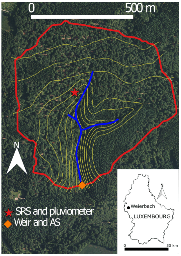
Figure 1Map of the Weierbach catchment and its location in Luxembourg. The weir is located at coordinates (5^∘47^′44^′′ E, 49^∘49^′38^′′ N). SRS is the sequential rainfall sampler. AS is the stream autosampler. The elevation lines increase by 5 m, from 460 m above sea level (a.s.l.) downstream close to the weir location to 510 m a.s.l. at the northern catchment divide.

Based on previous modeling (e.g., Fenicia et al., 2014; Glaser et al., 2019) and experimental studies (e.g., Martínez-Carreras et al., 2016; Juilleret et al., 2016; Scaini et al., 2017; Glaser et al., 2018), Rodriguez and Klaus (2019) proposed a perceptual model of streamflow generation in the Weierbach catchment. In this model, the first and flashy peaks of double-peaked hydrographs are generated by precipitation falling directly into the stream, by saturation excess flow from the near-stream soils, and by infiltration excess overland flow in the riparian area. The second peaks are generated by delayed lateral subsurface flow. The lateral fluxes are assumed higher at the PPSD/bedrock interface due to the hydraulic conductivity contrasts (Glaser et al., 2016, 2019; Loritz et al., 2017). Lateral subsurface flows are, thus, accelerated when groundwater rises after a rapid vertical infiltration through the soils (Rodriguez and Klaus, 2019). The model based on travel times presented in this study was developed in a step-wise manner, based on this hypothesis of streamflow generation, and the consistency between simulated and observed δ²H points toward a robust representation of the key processes. Water flow paths and streamflow-generation processes in this catchment are, however, not completely resolved. Other studies carried out in the Colpach catchment (containing the Weierbach) suggested that the first peaks are caused by a lateral subsurface flow through a highly conductive soil layer, and that second peaks are caused by groundwater flow in the bedrock (Angermann et al., 2017; Loritz et al., 2017). This is contrary to the conclusions from other studies in the Weierbach catchment (Glaser et al., 2016, 2020), showing that the key processes are still under debate.

2.2 Hydrometric and tracer data

In this study, we use precipitation (J; in mm h⁻¹), ET (mm h⁻¹), Q (mm h⁻¹), and δ²H (‰) and ³H (tritium units – TUs) measurements in precipitation (C_P,2 and C_P,3, respectively) and streamflow (C_Q,2 and C_Q,3, respectively). Here, the subscript 2 indicates deuterium (²H) and the subscript 3 indicates tritium (³H). The analysis in this study focuses on the period October 2015–October 2017 (Fig. 2). Details on the hydrometric data collection (J, ET, and Q), and on the ²H sample collection and analysis are given in Rodriguez and Klaus (2019).

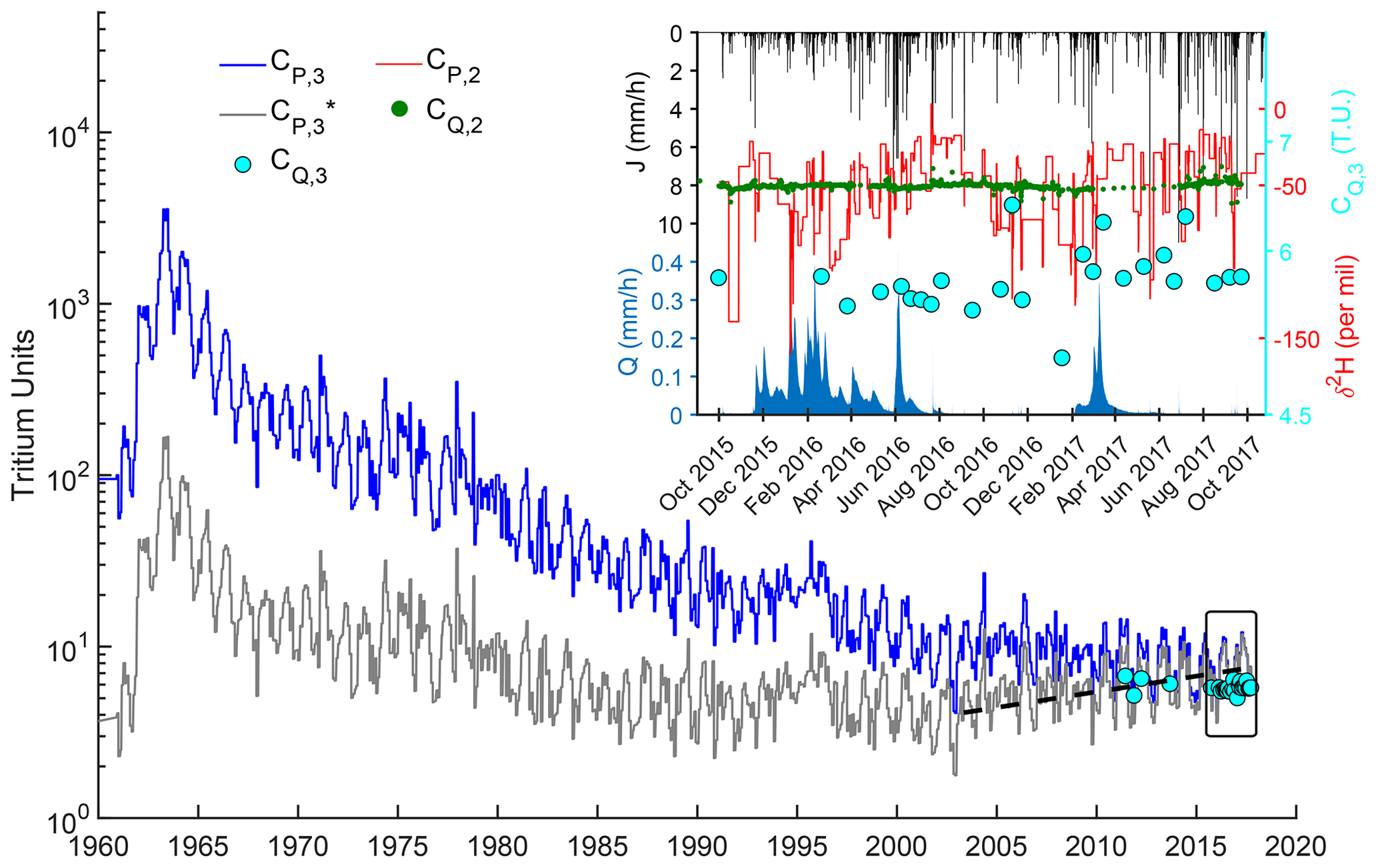
Figure 2Data used in this study – ³H in precipitation (C_P,3), the corresponding tritium activities accounting for radioactive decay until 2017 ($C_{\mathrm{P},\mathrm{3}}^{*}$), δ²H in precipitation C_P,2 (inset), precipitation J (inset), streamflow Q (inset), ³H measurements in the stream (C_Q,3 – both plots), and δ²H in the stream (C_Q,2; inset). The period contained in the inset is represented as a rectangle in the bigger plot. The dashed line visually represents the increasing trend in $C_{\mathrm{P},\mathrm{3}}^{*}$ that emerges as the effect of bomb peak tritium disappears (i.e., $C_{\mathrm{P},\mathrm{3}}(t-T)$ stops decreasing approximately from the year 2000 on, so $C_{\mathrm{P},\mathrm{3}}^{*}(T,t)=C_{\mathrm{P},\mathrm{3}}(t-T)e^{-\mathit{\alpha }T}$ starts decreasing with increasing T).

Download

The 1088 stream grab samples analyzed for ²H were instantaneous samples collected manually or automatically with an autosampler (AS; Fig. 1), resulting in samples taken, on average, every 15 h over October 2015–October 2017. These stream samples represent most flow conditions in the catchment in terms of frequency of occurrence (Fig. 3). The 525 precipitation samples analyzed for ²H were collected approximately every 2.5 mm rain increment (i.e., every 23 h on average) with a sequential rainfall sampler (SRS) and, in addition, as cumulative bulk samples on an approximately biweekly basis (but ranging from 1 to 4 weeks in some occasions). Both the sequential rainfall samples and the cumulative bulk samples represent a precipitation-weighted average δ²H over different time intervals (approximately daily intervals for sequential rainfall samples and approximately biweekly intervals for bulk samples). The samples were analyzed at the Luxembourg Institute of Science and Technology (LIST), using a Los Gatos Research (LGR) isotope water analyzer, yielding an analytical accuracy of 0.5 ‰ (equal to the LGR standard accuracy) for ²H and a precision-maintained <0.5 ‰ (quantified as 1 standard deviation of the measured samples and standards).

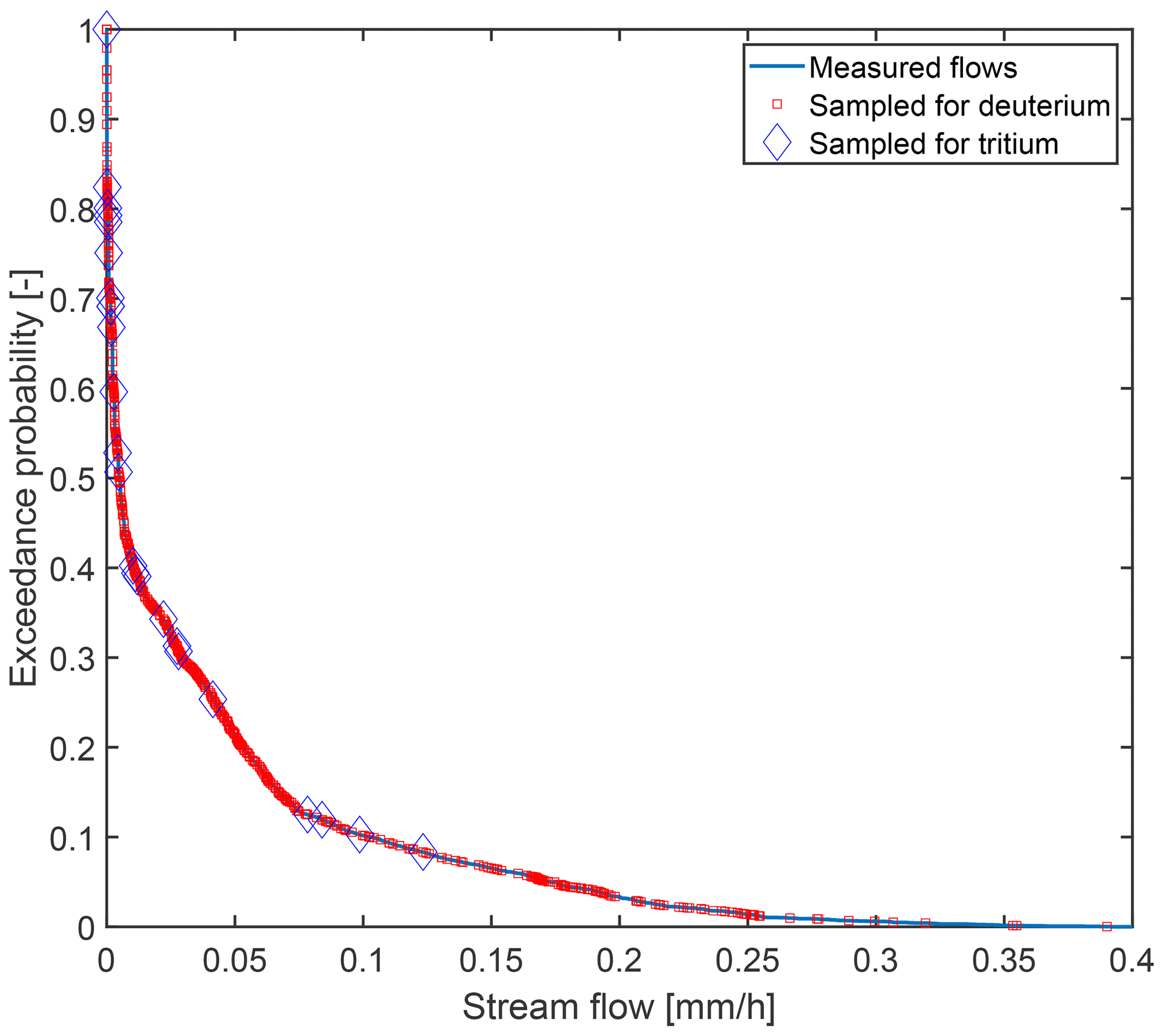
Figure 3Distribution of stream samples (³H and δ²H) along the flow exceedance probability curve defined as the fraction of streamflows exceeding a given value over 2015–2017.

Download

The 24 stream samples analyzed for ³H were instantaneous grab samples selected from manual biweekly sampling campaigns to cover various flow ranges. The manual selection was not based on flows ranked by exceedance probabilities but rather on the streamflow time series itself. The selected samples represent various hydrological conditions (e.g., the beginning of a wet period after a long dry spell or small but flashy streamflow responses) based on data available for this catchment (see Sect. 2 and Rodriguez and Klaus, 2019). The 24 tritium samples cover a wide portion of the flow frequencies (see Fig. 3; all sampled flow conditions occurred more than 90 % of the time). This number of ³H samples is one of the highest used in travel time studies (see Małoszewski and Zuber, 1993; Uhlenbrook et al., 2002; Stewart et al., 2007; Gallart et al., 2016; Gabrielli et al., 2018; Visser et al., 2019), and it is limited by the analytical costs. The samples were analyzed by the GNS Science water dating laboratory (Lower Hutt, New Zealand), which provides high-precision tritium measurements using electrolytic enrichment and liquid scintillation counting (Morgenstern and Taylor, 2009). The precision of the stream samples varies from roughly 0.07 TU to roughly 0.3 TU, but it is usually around 0.1 TU. ³H in the precipitation was obtained for the Trier station (Global Network of Isotopes in Precipitation, GNIP, station; 60 km away from the Weierbach) until 2016 from the WISER database of the International Atomic Energy Agency (IAEA; IAEA and WMO, 2019; Stumpp et al., 2014). The 2017 values were obtained from the radiology group of the Bundesanstalt für Gewässerkunde (Schmidt et al., 2020). ³H in precipitation before 1978 was calculated by regression with data from Vienna, Austria (Stewart et al., 2017). ³H in precipitation obtained from the IAEA corresponds to monthly integrated sampling made with an evaporation-free rain totalizer, as described in the GNIP station operations manual.

Since the stream grab samples were collected over a short time interval (seconds to minutes) using a weir, the associated concentrations, C_Q,2(t) and C_Q,3(t), represent the instantaneous value of the deuterium and tritium concentrations in the stream at time t, equivalent to the concept of flux concentrations in Kreft and Zuber (1978) and Małoszewski and Zuber (1982). For both ²H and ³H, the time series of tracer in precipitation was interpolated between two consecutive samples (e.g., A and B) as being equal to the value of the next sample (i.e., B). This was necessary in order to obtain a continuous tracer input time series (required for Eq. (1) to work). For ²H, the signal obtained from cumulative bulk samples was continuous by design and, thus, used as a baseline representing the steps of constant δ²H over 2 weeks on average. Then, the discontinuous signal with higher frequency variations provided by the sequential rainfall samples was inserted into the continuous baseline for the periods when sequential rainfall samples were available (this higher frequency signal is not continuous because of the periods of the absence of samples when the SRS failed). Therefore, in this study, C_P,2(t) represents the instantaneous value of δ²H in precipitation at time t, equal to the precipitation-weighted average value over varying time intervals. Also, C_P,3(t) represents the instantaneous value of ³H in precipitation at time t, equal to the precipitation-weighted average value over monthly intervals. Assuming uniform precipitation over the catchment, C_P,2(t) and C_P,3(t) are also equivalent to flux concentrations (Małoszewski and Zuber, 1982). Since no measurements of J, Q, ET, and C_P,2 are available before 2010, we periodically looped back their values from the period of October 2010–October 2015 for the time period before 2010 as a best estimate of their past values (Figs. S16 and S17). We aggregated the input data (J, ET, Q, C_P,2, and C_P,3) to a resolution Δt=4 h, which is small enough to capture the variability in the flows and tracers in the input and simulate the variability in the flows and tracers in the output.

2.3 Mathematical framework

Mathematically, the streamflow TTD is related to the stream tracer concentrations C_Q(t), according to the following Eq. (1):

where T is the travel time (the age of water at the outlet), t is time of observation, C_Q(t) is the stream tracer concentration, $\begin{array}{c}\leftarrow \\ {\mathit{p}}_Q\end{array}$ (probability distribution function – pdf) is the stream backward TTD (Benettin et al., 2015b), and $C_{\mathrm{P}}^{*}(T,t)$ is the tracer concentration of the water parcel reaching the outlet at time t with travel time T (this parcel was in the inflow at time t−T). The concentrations in this equation need to be flux concentrations, i.e., representative of the tracer mass fluxes in inflows and outflows (see Sect. 2.2). This equation is always true for the exact (usually unknown) TTD because it simply expresses the fact that the stream concentration is the volume-weighted arithmetic mean of the concentrations of the water parcels with different travel times at the outlet (the weighting of tracer concentrations by hydrological fluxes is thus implicit in $\begin{array}{c}\leftarrow \\ {\mathit{p}}_Q\end{array}(T,t)$). Thus, contrary to most of the past travel time studies using a steady-state version of Eq. (1), no weighting of the concentrations by fluxes is necessary because the time-varying TTD $\begin{array}{c}\leftarrow \\ {\mathit{p}}_Q\end{array}(T,t)$ already accounts for the time-varying fractions of precipitation not reaching the stream (due to either ET or storage; see Sect. 2.4) and for time-varying streamflow rates. $C_{\mathrm{P}}^{*}(T,t)$ depends on T and t as separate variables if the tracer concentration of a water parcel in the catchment changes between injection time t−T and observation time t. For solutes like silicon and sodium, the concentration can increase with travel time (Benettin et al., 2015a). For ³H, radioactive decay with a constant α=0.0563 yr⁻¹ implies $C_{\mathrm{P},\mathrm{3}}^{*}(T,t)=C_{\mathrm{P},\mathrm{3}}(t-T)e^{-\mathit{\alpha }T}$, where $C_{\mathrm{P},\mathrm{3}}(t-T)$ is the concentration in precipitation measured at t−T. For ²H, $C_{\mathrm{P},\mathrm{2}}^{*}(T,t)=C_{\mathrm{P},\mathrm{2}}(t-T)$. Thus, the streamflow TTD simultaneously verifies Eqs. (2) and (3) as follows:

Practically, when measurements of ²H and ³H are used to inversely deduce the TTD by using Eqs. (2) and (3), different TTDs may be found. These different TTDs may be called $\begin{array}{c}\leftarrow \\ {\mathit{p}}_{Q,\mathrm{2}}\end{array}$ and $\begin{array}{c}\leftarrow \\ {\mathit{p}}_{Q,\mathrm{3}}\end{array}$ for instance, referring to ²H and ³H, respectively. To avoid introducing more variables and to avoid confusion, we do not use the names $\begin{array}{c}\leftarrow \\ {\mathit{p}}_{Q,\mathrm{2}}\end{array}$ and $\begin{array}{c}\leftarrow \\ {\mathit{p}}_{Q,\mathrm{3}}\end{array}$, and we instead refer to the TTDs constrained by a given tracer using a common symbol $\begin{array}{c}\leftarrow \\ {\mathit{p}}_Q\end{array}$. We do this also to stress that the exact (true) TTD must simultaneously verify both Eqs. (2) and (3), and that two different TTDs $\begin{array}{c}\leftarrow \\ {\mathit{p}}_{Q,\mathrm{2}}\end{array}$ and $\begin{array}{c}\leftarrow \\ {\mathit{p}}_{Q,\mathrm{3}}\end{array}$ cannot physically exist. This is a fundamental difference from previous work that assumed two different TTDs, using for example Eq. (3) for ³H and another method for ²H (the sine wave approach; e.g., Małoszewski et al., 1983). The framework in this study also uses the fact that the same functional form of streamflow TTD needs to simultaneously explain both tracers to be valid, unlike previous work that used different TTD models for different tracers (Stewart and Thomas, 2008).

2.4 Transport model based on TTDs

Most of the previous travel time studies using tritium assumed steady-state flow conditions and an analytical shape for the streamflow TTD and fitted the parameters of the analytical function using the framework described in Sect. 2.3. In this study, the TTDs are unsteady (i.e., time varying or transient) and cannot be analytically described. Still, they can be calculated by numerically solving the master equation (Botter et al., 2011). This method has been applied in several recent studies (e.g., van der Velde et al., 2015; Harman, 2015; Benettin et al., 2017b) and is described in more detail by Benettin and Bertuzzo (2018). The numerical method used to solve this equation in this study is described by Rodriguez and Klaus (2019). The biggest difference, compared to many previous travel time studies, is that time-varying TTDs can be obtained from the master equation without using tracer information (i.e., Eqs. 2 and 3). In this case, tracer equations (Eqs. 2 and 3) simply become a constraint on the solutions found by solving the master equation.

Essentially, the master equation is a water balance equation in which storage and fluxes are labeled with age categories. The master equation is thus a partial differential equation. It expresses the fact that the amount of water in storage, with a given residence time, changes with calendar time. This change is due to new water introduced by precipitation J(t), water aging, and losses to catchment outflows ET(t) and Q(t). Solving the master equation requires knowledge (or an assumption about the shape) of the SAS functions Ω_Q and Ω_ET of outflows Q and ET, which conceptually represent how likely it is that water ages in storage (residence times) are to be present in the outflows at a given time. Solving the master equation yields the distribution of residence times in storage at every moment that can be represented in a cumulative form with age-ranked storage S_T. It is defined as the amount of water in storage (e.g., 10 mm) younger than T (e.g., 1 year) at time t. T→S_T is just a mathematical change of a variable, and it has no meaning respective to the location or depth of a water parcel with a certain residence time in the catchment. By definition $\underset{T\to +\mathrm{\infty }}{lim}{S}_T=S\left(t\right)$, where S(t) is catchment storage. Ω_Q and Ω_ET are functions of S_T and cumulative distributions functions (cdf's) for numerical convenience. SAS functions are closely linked to TTDs, such that one can be found from the other using the following expression (here it has been used for Q, but it is also valid for other outflows):

The partial derivative with respect to travel time T ensures the transition from cdf to pdf. Assuming a parameterized form for Ω_Q and Ω_ET, and calibrating their parameters using the framework defined in Sect. 2.3, yields time-varying TTDs constrained by the tracers in the outflows. In this study, the parameters of Ω_Q are directly calibrated by using Eq. (1) for C_Q. Since no tracer data C_ET are available, the parameters of Ω_ET are indirectly deduced from Eq. (1) using the tracer measurements in streamflow only. This is made possible by the indirect influence of Ω_ET on the tracer partitioning between Q and ET and on the tracer mass balance (Appendix A2).

We assumed that Ω_ET is a function of only S_T, and it is gamma distributed with a mean parameter μ_ET (in millimeters) and a scale parameter θ_ET (in millimeters). Rodriguez and Klaus (2019) showed that, in the Weierbach catchment, a weighted sum of three components in the streamflow SAS function is more consistent with the superposition of streamflow-generation processes (i.e., saturation excess flow, saturation overland flow, and lateral subsurface flow; see Sect. 2.1) than a single component. This means that Ω_Q is written as a weighted sum of three cdf's (see Appendix A1; Rodriguez and Klaus, 2019) as follows:

λ₁(t), λ₂(t), and λ₃(t) are time-varying weights summing to one. λ₁(t) is parameterized to sharply increase during flashy streamflow events, using parameters ${\mathit{\lambda }}_{\mathrm{1}}^{*}$, f₀, S_th (in millimeters), and ΔS_th (in millimeters; see Appendix A1). λ₂(t)=λ₂ is calibrated, and λ₃(t) is just deduced by difference. Ω₁ is a cumulative uniform distribution over S_T in [0, S_u] (with S_u a parameter in millimeters). Ω₁ represents the young water contributions associated with short flow paths during flashy streamflow events. We chose rather low values of ${\mathit{\lambda }}_{\mathrm{1}}^{*}$ (see Table 1), such that λ₁(t) is generally the smallest weight (because ${\mathit{\lambda }}_{\mathrm{1}}\left(t\right)\le {\mathit{\lambda }}_{\mathrm{1}}^{*}$). The lower values of λ₁(t) compared to other weights are consistent with tracer data, suggesting limited contributions of event water to streamflow (Martínez-Carreras et al., 2015; Wrede et al., 2015). Ω₁ corresponds to the following processes in the near-stream area: saturation excess flow, saturation overland flow, and rain on the stream (Rodriguez and Klaus, 2019). Ω₂ and Ω₃ are gamma distributed, with mean parameters μ₂ and μ₃ (in millimeters) and scale parameters θ₂ and θ₃ (in millimeters), respectively. Ω₂ and Ω₃ represent older water that is always contributing to the stream. This older water consists of groundwater stored in the weathered bedrock that flows laterally in the subsurface. Note that we used the same functional form of Ω_Q(S_T,t) for ²H and ³H to keep the functional form of the TTDs consistent between the tracers. Although composite SAS functions may considerably increase the complexity of the model compared to traditional SAS functions, they are necessary to account for different streamflow-generation processes (Rodriguez and Klaus, 2019). These processes are potentially associated with contrasting flow path lengths and/or water velocities, hence the contrasting travel times. The accurate representation of these contrasting travel times is most likely vital for reliable simulations of stream chemistry (Rodriguez et al., 2020).

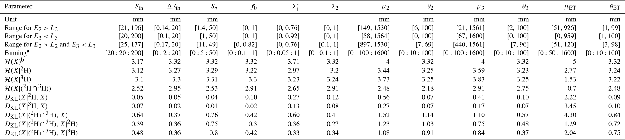
Table 1Model parameters.

^a Details about the equations involving these parameters are given in Appendix A1 and in Rodriguez and Klaus (2019). ^b ${\mathit{\lambda }}_{\mathrm{1}}^{*}$ is, in fact, uniformly sampled between 0 and $\mathrm{1}-{\mathit{\lambda }}_{\mathrm{2}}\le \mathrm{1}$ to ensure that $\sum _{n=\mathrm{1}}^{\mathrm{3}}{\mathit{\lambda }}_k\left(t\right)=\mathrm{1}$. This also ensures that values close to 0 are more often sampled than values close to 1 for ${\mathit{\lambda }}_{\mathrm{1}}^{*}$. ^c λ₁(t) varies, λ₂ is constant, and λ₃(t) varies, and it is deduced using ${\mathit{\lambda }}_{\mathrm{3}}\left(t\right)=\mathrm{1}-{\mathit{\lambda }}_{\mathrm{2}}-{\mathit{\lambda }}_{\mathrm{1}}\left(t\right)$.

Download Print Version | Download XLSX

2.5 Model initialization and numerical details

Numerically solving the master equation requires an estimation of catchment mobile storage S(t). Here, S(t) represents the sum of dynamic (or active) storage and inactive (or passive) storage (Fenicia et al., 2010; Birkel et al., 2011; Soulsby et al., 2011; Hrachowitz et al., 2013). In this study, the model is initialized with storage $S(t=\mathrm{0})=S_{\mathrm{ref}}=\mathrm{2000}$ mm. This initial value is chosen to be large enough to sustain Q and ET during drier periods and to store water that is sufficiently old to satisfy Eq. (1). S(t) is then simply deduced from the water balance as $S\left(t\right)=S_{\mathrm{ref}}+\underset{x=\mathrm{0}}{\overset{t}{\int }}\left(J\right(x)-Q(x)-\mathrm{ET}(x\left)\right)\mathrm{d}x$. The initial residence time distribution in storage p_S(T,t) is exponential with a mean of 1.7 years, the mean residence time (MRT) by Pfister et al. (2017). Initial conditions need not be specified for the SAS functions, since these are directly calculated from the initial state variables ($S_T(t=\mathrm{0})=S(t=\mathrm{0})\underset{x=\mathrm{0}}{\overset{T}{\int }}{\mathit{p}}_{\mathrm{S}}(x,t=\mathrm{0})\mathrm{d}x$), assuming a parametric form and a set of parameter values. The model is then run with the time steps Δt=4 h and age resolution ΔT=8 h. In this way, the computational cost is balanced with the resolution of the simulations in δ²H. A 100-year spin-up is used to numerically allow the presence of water of up to 100 years old in storage and to avoid a numerical truncation of the TTDs. This spin-up is also long enough to completely remove the impact of the initial conditions. This means that S_ref and the initial residence time distribution in storage do not influence the results over October 2015–October 2017. ET(t) is taken to be equal to potential evapotranspiration PET(t), except that it tends nonlinearly towards 0 (using a constant smoothing parameter n) when storage S(t) decreases below S_root (in millimeters) and where S_root is a parameter accounting for the water amount accessible by ET (Appendix A2).

2.6 Model calibration

The parameters of the SAS functions and the other model parameters were calibrated using a Monte Carlo technique. In total, 12 parameters were calibrated (Table 1). The initial ranges were selected based on parameter feasible values (e.g., f₀ between 0 and 1 by definition), on previous estimations (e.g., S_th), on hydrological data (e.g., S_u and ΔS_th deduced from average precipitation depths), and on initial tests done on the parameter ranges (e.g., μ and θ). These ranges allow a wide range of shapes of SAS functions, while minimizing numerical errors (occurring, for example, for S_T>S(t)).

Unlike our previous modeling work in this catchment (Rodriguez and Klaus, 2019), we fixed the initial storage in the model S_ref (to 2000 mm). We did this to reduce the degrees of freedom when sampling the parameter space in order to limit the impact of numerical errors on the calibration. These errors are due to the numerical truncation of Ω_Q(S_T,t) when a considerable part (e.g., a few percent) of its tail extends above S(t). This occurs when parameters μ₂, μ₃, θ₂, and θ₃ are too large compared to S_ref when the latter is also randomly sampled. Choosing a constant large value for S_ref thus guarantees the absence of truncation errors. S_ref has little influence on the storage deduced from travel times, since the ages sampled from storage by streamflow are governed only by μ₂, μ₃, θ₂, and θ₃. These parameters are independent of S_ref as long at it allows sufficiently old water to reside in storage, which is ensured by its large value and by the long spin-up period we used (100 years).

The first step in the Monte Carlo procedure consisted of randomly sampling parameters from the uniform prior distributions with the ranges defined in Table 1. A total of 12 096 sets of the 12 calibrated parameters were sampled as a Latin hypercube (LHS; Helton and Davis, 2003). This sampling technique has the advantages of a stratified sampling technique and the simplicity and objectivity of a purely random sampling technique (Helton and Davis, 2003). It was chosen to make sure that the parameter samples are as evenly distributed as possible, despite their relatively small number with respect to the high number of dimensions (due to computational constraints enhanced by the required long spin-up period). The model was then run over the 100-year spin-up followed by October 2015–October 2017, and its performance was evaluated over October 2015–October 2017. We evaluated model performance in a multi-objective manner, by using separate objective functions for ²H and ³H. For deuterium, we used the Nash–Sutcliffe efficiency (NSE) as follows:

where N₂=1016 is the number of deuterium observations in the stream. For tritium, we used the mean absolute error (MAE) as follows:

where N₃=24 is the number of tritium observations in the stream. We used the MAE for tritium because it is common to report errors in TU and because of the limited variance in stream ³H (due to the limited number of samples and the low variability), making the NSE less appropriate (Gallart et al., 2016). The behavioral parameter sets that are used for uncertainty calculations and further analysis were selected based on threshold values L₂ and L₃ for the performance measures E₂ and E₃, respectively (Beven and Binley, 1992). Parameter sets were considered behavioral for deuterium simulations, if $E_{\mathrm{2}}>L_{\mathrm{2}}=\mathrm{0}$, and behavioral for tritium simulations, if $E_{\mathrm{3}}<L_{\mathrm{3}}=\mathrm{0.5}$ TU. We subsequently refer to these parameter sets and corresponding simulations as constrained by deuterium, constrained by tritium, and constrained by both when both performance criteria were used. We chose these constraints to obtain reasonable model fits to the data, to obtain a comparable number of behavioral parameter sets for ²H and ³H, and to maximize the amount of information gained about the parameters when adding a constraint on the model performance for a tracer. This information gain was assessed with the Kullback–Leibler divergence D_KL between the parameter distributions inferred from various combinations of constraints L₂ and L₃ (Sect. 2.7).

2.7 Information contents of ²H and ³H

Loritz et al. (2018, 2019) recently used information theory to detect the hydrological similarity between hillslopes of the Colpach catchment and to compare topographic indexes in the Attert catchment in Luxembourg. Thiesen et al. (2019) used information theory to build an efficient predictor of rainfall–runoff events. In this study, we leverage information theory to evaluate our model parameter uncertainty (Beven and Binley, 1992) and to assess the added value of δ²H and ³H tracers for information gains on travel times. First, we calculated the expected information content of the prior and posterior parameter distributions, using the Shannon entropy ℋ as follows:

In this equation, the parameter X (e.g., μ₂) takes values (e.g., 125 mm) falling in intervals I_k (e.g., [100, 150] mm) that do not intersect each other and which union ${\cup }_{k=\mathrm{1}}^{n_{\mathrm{I}}}{I}_k$ equals I_X, the total interval of values on which X is defined (e.g., [50, 500] mm). The definitions of the n_I intervals I_k for each parameter depend on the binning of the parameter values (given in Table 2). The distribution f defines the probability of the parameter X to be in a certain state (i.e., to take a value falling in an interval I_k) when constrained by the criterion $E_{\mathrm{2}}>L_{\mathrm{2}}(i=\mathrm{2})$ or $E_{\mathrm{3}}<L_{\mathrm{3}}(i=\mathrm{3})$ (posterior distribution) or none of those (prior distribution). f can also be calculated for a combination of these criteria ($\mathcal{H}\left(X\right|({}^{\mathrm{2}}\mathrm{H}\cap {}^{\mathrm{3}}\mathrm{H}))$). When using the logarithm of base 2, ℋ is expressed in bits of information contained in the distribution f. The uniform distribution over I_X has the maximum possible entropy. Lower values of ℋ thus indicate that the distribution is not flat; hence, it is less uncertain than the uniform prior distribution. In general, lower values of ℋ indicate lower parameter uncertainty. Lower values of ℋ for the posteriors also indicate that information on travel times was extracted from the tracer time series. We used the Kullback–Leibler divergence D_KL to precisely evaluate the information gain from prior to posterior distributions as follows:

where f is the posterior distribution constrained by E₂>L₂ and/or E₃<L₃, and g is the prior distribution. D_KL is expressed in bits of information gained when the knowledge about a parameter distribution is updated by using tracer data. Summing the $D_{\mathrm{KL}}(X{|}^i\mathrm{H},X)$ for all the parameters and for a given tracer (i=2 or i=3) yields the total amount of information learned on travel times from that tracer. We also used the Kullback–Leibler divergence D_KL to evaluate the gain of information when ³H is used in addition to ²H to constrain model predictions, or vice versa, in the following:

where f is the posterior distribution constrained by E₂>L₂ and E₃<L₃, and g is the posterior distribution constrained only by $E_{\mathrm{2}}>L_{\mathrm{2}}(i=\mathrm{2})$ or only by $E_{\mathrm{3}}<L_{\mathrm{3}}(i=\mathrm{3})$. D_KL is expressed in bits of information gained when the knowledge about a parameter posterior distribution is updated by adding another tracer. Calculating D_KL also requires binning the parameter values to define the intervals I_k and calculate the distributions f and g. The binning for each parameter (Table 2) was chosen such that the resulting histograms visually reveal the underlying structure of the parameter values, while avoiding uneven features and irregularities (e.g., very spiky histograms).

3.1 Calibration results

A total of 148 parameter sets were behavioral for deuterium simulations, with E₂ ranging from L₂=0 to 0.24. A total of 181 parameter sets were behavioral for tritium simulations, with E₃ ranging from 0.24 to L₃=0.5 TU. Additionally, 16 parameter sets were behavioral for both tritium and deuterium simulations, with E₂ ranging from L₂=0 to 0.19 and E₃ ranging from 0.36 to L₃=0.5 TU. These solutions show that a reasonable agreement between the model fit to ²H and the model fit to ³H can be found.

The behavioral posterior parameter distributions constrained by deuterium or tritium or by both generally had similar ranges to their prior distributions, except, notably, for μ₂, θ₂, μ₃, and θ₃ (Table 2). To assess the reduction in parameter uncertainty, we calculated and compared the entropy of the prior and of the posterior distributions (Table 2). A visual inspection of the posterior distributions was also made. Here, we show only the parameters μ₂, θ₂, μ₃, and θ₃ (Fig. 4) that directly control the range of longer travel times in streamflow, since they act mostly on the right-hand tail of the gamma components in Ω_Q. These parameters thus have a direct influence on the catchment storage inferred via age-ranked storage S_T. The distributions of μ₂, θ₂, μ₃, and θ₃ are clearly not uniform. The distributions of the other parameters are provided in the Supplement (Figs. S12 and S13). Most distributions are not uniform, indicating that the parameters are identifiable.

Table 2Parameter ranges and information measures before and after calibration to isotopic data.

^a Binning is indicated as $[a:b:c]$, where a is the left edge of the first bin, b is the bin width, and c is the right edge of the last bin. For instance, $[\mathrm{7}:\mathrm{2}:\mathrm{11}]$ indicates data sorted with the two bins [7, 9] and [9, 11]. ^b ℋ and D_KL are expressed in bits.

Download Print Version | Download XLSX

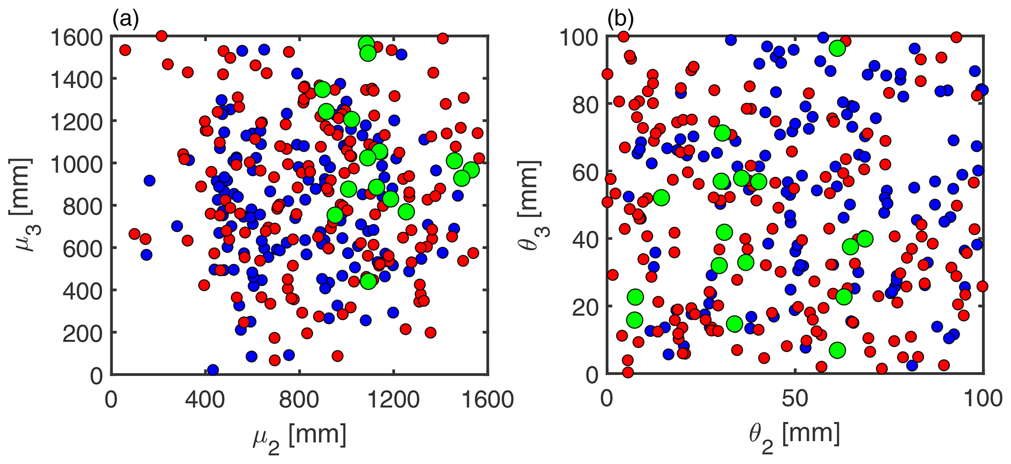
Figure 4Distributions of SAS function mean (μ; a) and scale (θ; b) behavioral parameters directly controlling the selection of longer travel times by streamflow, constrained by deuterium (148 blue dots) or tritium (181 red dots) or both (16 green dots).

Download

Essentially, the results (Table 2 and Fig. 4) reveal that the parameter ranges decreased by adding information on ²H or ³H or both. This effect is particularly noticeable for f₀ and ${\mathit{\lambda }}_{\mathrm{1}}^{*}$, which saw their upper boundary decrease, and for μ₂ and μ₃, which saw their lower boundary increase considerably. These results also show that the posterior distributions depart from the uniform prior distributions when considering ²H alone or ³H alone (i.e., $\mathcal{H}\left(X{|}^i\mathrm{H}\right)<\mathcal{H}\left(X\right)$ and $D_{\mathrm{KL}}(X{|}^i\mathrm{H},X)>\mathrm{0}$ in Table 2). This effect is not very pronounced for most parameters, but it is clearly visible for ${\mathit{\lambda }}_{\mathrm{1}}^{*}$, μ₂ and μ₃ (e.g., uneven distributions of points in Fig. 4), and for μ_ET. The posterior distributions become considerably narrower when both tracers are considered, since $\mathcal{H}\left(X\right|({}^{\mathrm{2}}\mathrm{H}\cap {}^{\mathrm{3}}\mathrm{H}))$ is much lower than ℋ(X), which is visually represented by the distribution of points tending to cluster towards a corner in Fig. 4. Generally, more was learned about the likely parameter values by adding a constraint on ²H simulations after constraining ³H simulations to the opposite (i.e., generally $D_{\mathrm{KL}}\left(X\right({}^{\mathrm{2}}\mathrm{H}\cap {}^{\mathrm{3}}\mathrm{H}),X|{}^{\mathrm{3}}\mathrm{H})\ge D_{\mathrm{KL}}(X\left|\right({}^{\mathrm{2}}\mathrm{H}\cap {}^{\mathrm{3}}\mathrm{H}),X|{}^{\mathrm{2}}\mathrm{H})$). Noticeable exceptions to this are the parameters μ₂, θ₂, and θ₃, which are more related to the longer travel times in streamflow and to catchment storage than the other parameters.

Simulations of stream δ²H captured both the slow and the fast dynamics of the observations when constrained by E₂>0 (blue bands and blue curve in Fig. 5a), although some variability is not fully reproduced. The Nash–Sutcliffe efficiency (E₂) is limited to 0.24 despite visually satisfying simulations (Sect. 4.4.2). Most flashy responses in δ²H (associated with flashy streamflow responses) were reproduced to some extent by the behavioral simulations (the very thin peaks of the blue bands in Fig. 5a; more visible in Figs. S1–S9 in the Supplement). Nevertheless, about 3 % of δ²H data points were visibly underestimated, pointing at a partial limitation of the composite SAS functions to simulate the variability in the streamflow TTD at these few instances (see Sect. 4.4.2). Behavioral simulations that were selected using the other performance criterion instead (E₃<0.5 TU; red bands in Fig. 5) did not match the δ²H observations well. This shows that ³H contains some information on travel times that is not in common with ²H. Yet, these behavioral simulations are able to match all observed δ²H flashy responses in amplitude, suggesting that, like δ²H, ³H contains information on young water contributions to streamflow (Sect. 4.3). Additionally, δ²H simulations that were constrained by both criteria (green bands) have a smaller variability than those constrained only by E₂>0, suggesting that ³H contains some information that is common with ²H.

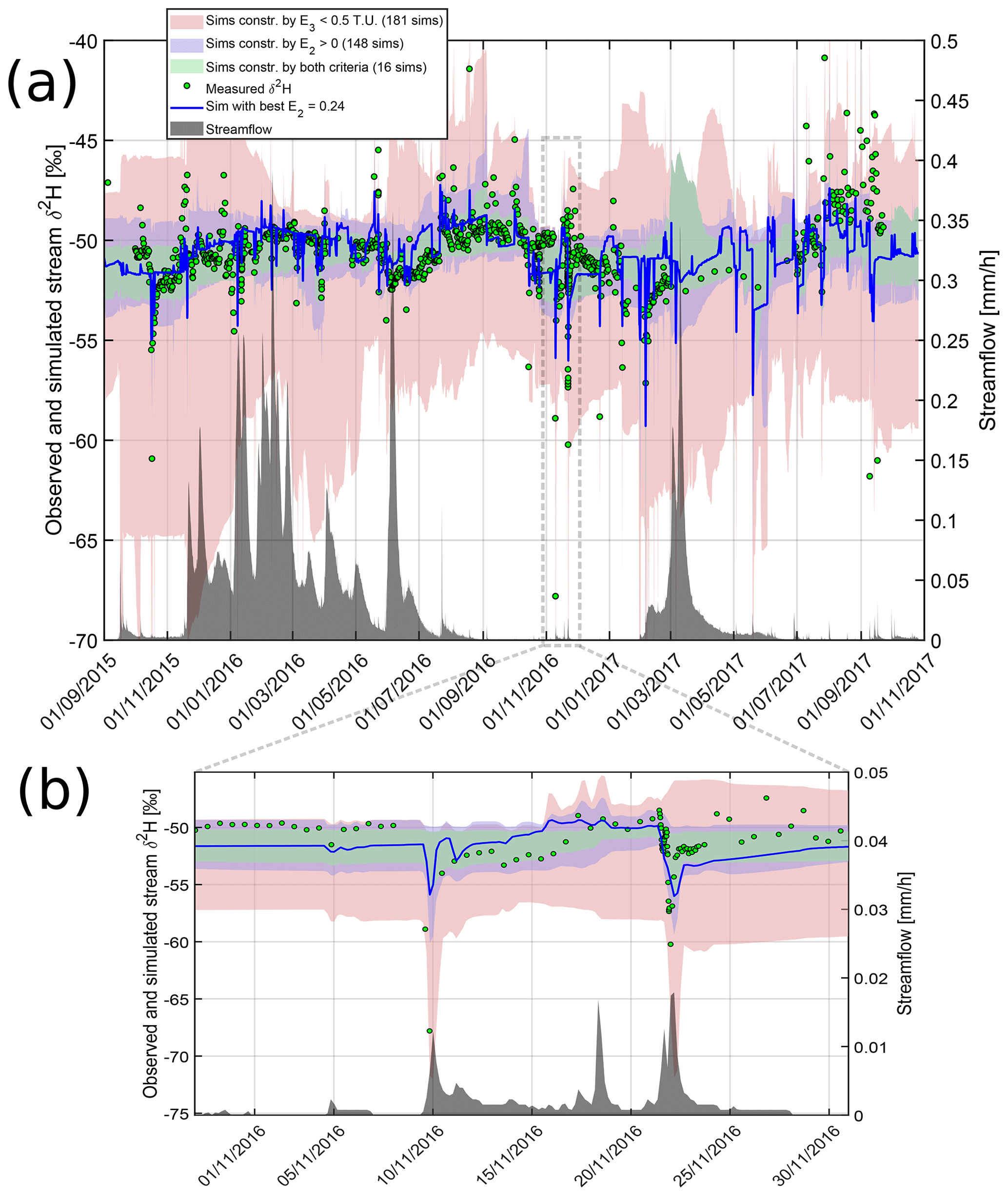
Figure 5Simulations in deuterium. E₂ is the Nash–Sutcliffe efficiency in deuterium, and E₃ is the mean absolute error in tritium units.

Download

Simulations of stream ³H generally matched the observations better in 2017 than before 2017 (red bands and red curve in Fig. 6). Some simulations (red bands) nevertheless matched the observations before 2017 relatively well. Similar to δ²H simulations, both the slow and the fast tracer responses seemed necessary to reproduce the variability in ³H observations (especially in 2017), although additional stream samples would be needed to confirm that the model is accurate between the current measurement points. The higher stream ³H values in 2017 that were better reproduced by the model correspond to an extended dry period during which streamflow responses were mostly flashy and short-lasting hydrographs. The ³H values in 2017 were closer to precipitation ³H, mostly around 10 TU (see also Fig. S15). The stream reaction to those higher values suggests a considerable influence of recent rainfall events on the stream. Steady-state TTD models relying only on tritium decay would probably struggle to simulate these fast responses. This also suggests a stronger influence of old water in 2016 than in 2017 (see Sect. 4.4.2). Simulations constrained by deuterium (blue bands) tended to overestimate stream ³H. Simulations constrained by both criteria (green bands) worked well in 2017, but they overestimated stream ³H before 2017. Similar to δ²H simulations, this suggests that ²H and ³H have common but also distinct information contents on travel times. The tendency of the model constrained by deuterium and/or by tritium to overestimate the tritium content in streamflow suggests a nonnegligible influence of the isotopic partitioning of inputs between Q and ET (Sect. 4.4.2; Appendix A2; Fig. S15).

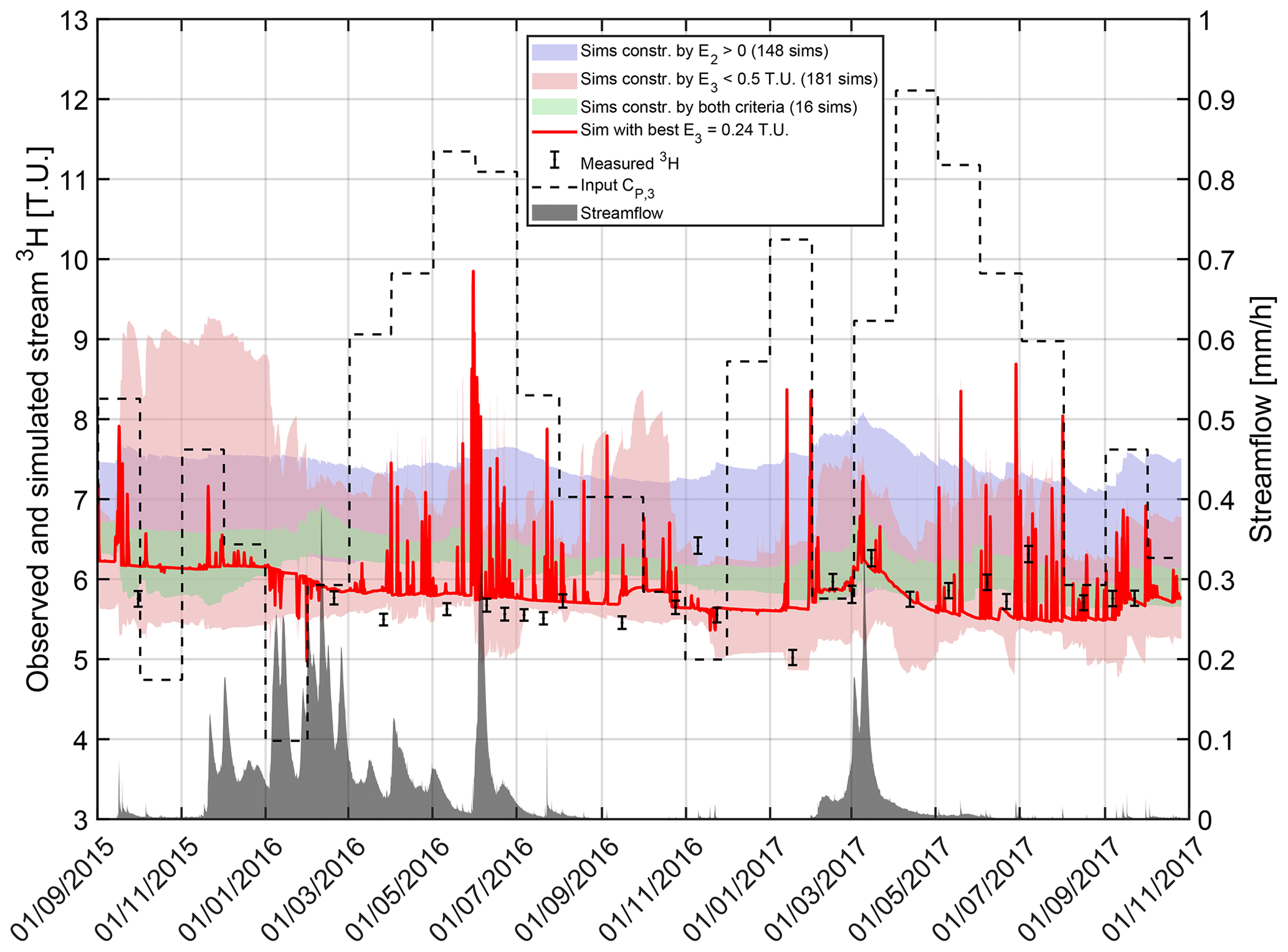
Figure 6Simulations of stream concentrations in tritium compared to observations of and variability in precipitation.

Download

3.2 Storage and travel time results

For each behavioral parameter set, we calculated $\begin{array}{c}\leftarrow \\ {\mathit{P}}_Q\end{array}\left(T\right)$, the average streamflow TTD weighted by Q(t) (over 2015–2017) in cumulative form (Fig. 7). Visually, there are no striking differences between $\begin{array}{c}\leftarrow \\ {\mathit{P}}_Q\end{array}\left(T\right)$ constrained by deuterium or by tritium, except a slightly wider spread for simulations constrained by tritium. The $\begin{array}{c}\leftarrow \\ {\mathit{P}}_Q\end{array}\left(T\right)$ constrained by both tracers clearly differ. The associated curves (Fig. 7c) show a much narrower spread. The travel time uncertainties are thus visually much lower than when using each tracer individually, highlighting the benefit of using both tracers together. The $\begin{array}{c}\leftarrow \\ {\mathit{P}}_Q\end{array}\left(T\right)$ constrained by both tracers also slightly shifted towards higher travel times. We calculated various statistics of the $\begin{array}{c}\leftarrow \\ {\mathit{P}}_Q\end{array}\left(T\right)$ constrained by the different performance criteria to quantitatively compare the distributions (Table 3). This showed that the $\begin{array}{c}\leftarrow \\ {\mathit{P}}_Q\end{array}\left(T\right)$ constrained only by tritium systematically corresponded to higher travel times (and lower young water fractions) than those constrained only by deuterium. A Wilcoxon rank sum test revealed that some statistically significant differences exist between the $\begin{array}{c}\leftarrow \\ {\mathit{P}}_Q\end{array}\left(T\right)$ constrained by deuterium and the $\begin{array}{c}\leftarrow \\ {\mathit{P}}_Q\end{array}\left(T\right)$ constrained by tritium (Appendix B). Even if these differences are statistically significant, they remain lower than in previous studies (Sect. 4.1). In addition, the youngest water fractions and the oldest water fractions of $\begin{array}{c}\leftarrow \\ {\mathit{P}}_Q\end{array}\left(T\right)$ did not significantly differ according to the Wilcoxon rank sum test (Appendix B).

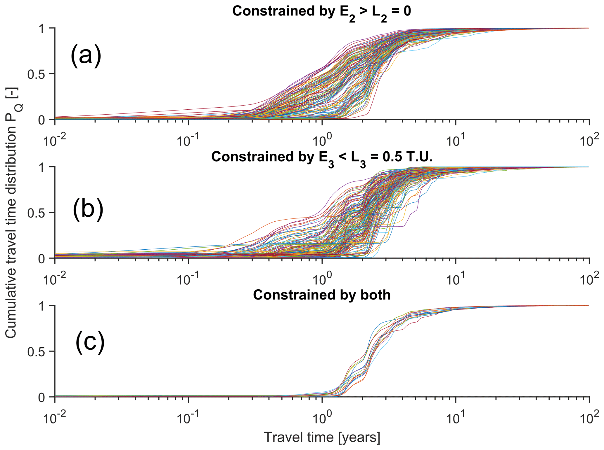
Figure 7Flow-weighted (2015–2017) cumulative stream TTDs for the behavioral parameter sets constrained by ²H (a), ³H (b), and both (c).

Download

Table 3Statistics of $\overleftarrow{{\mathit{P}}_Q}\left(T\right)$ constrained by deuterium or tritium.

The mean and standard deviations are calculated from all retained behavioral solutions for a given criterion. ^* Fraction of young water (Kirchner, 2016) that is younger than 0.2 years.

Download Print Version | Download XLSX

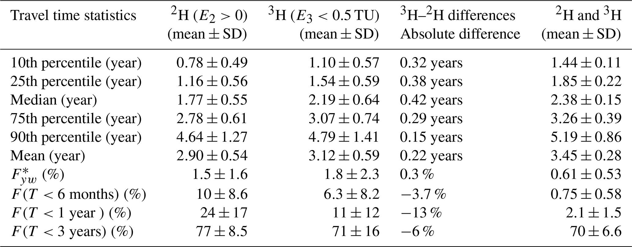
We defined the right-hand tail of the streamflow SAS function Ω_tail as being the weighted sum of the two gamma components in Ω_Q as follows:

where ${\mathit{\lambda }}_{\mathrm{3}}^{*}=\mathrm{1}-{\mathit{\lambda }}_{\mathrm{2}}-{\mathit{\lambda }}_{\mathrm{1}}^{*}$. Ω_tail thus allows us to study the asymptotic behavior of the function Ω_Q in detail. In particular, this asymptotic behavior is time invariant when plotted against S_T because Ω₂ and Ω₃ are functions of S_T only. The behavioral parameter sets were thus directly used to calculate the curves (S_T; Ω_tail(S_T)). These curves show similar differences for ²H and ³H to the curves (T; $\begin{array}{c}\leftarrow \\ {\mathit{P}}_Q\end{array}\left(T\right)$; see Fig. 8) because a slightly wider spread is observed for Ω_tail constrained by tritium than that constrained by deuterium (Fig. 8b), and the Ω_tail constrained by both tracers tend to converge to a narrow envelope of curves slightly shifted towards higher storage values (Fig. 8c).

Figure 8Cumulative right-hand tail Ω_tail of streamflow SAS functions for the behavioral parameter sets constrained by ²H (a), ³H (b), and both (c). Ω_tail is defined as the weighted sum of the two gamma components in Ω_Q. The black crosses indicate S_95P for each curve, i.e., the 95th percentile of Ω_tail.

Download

Table 4Storage estimate S_95P constrained by deuterium or tritium.

S_95P is calculated as the 95th percentile of Ω_tail (Eq. 11).

Download Print Version | Download XLSX

To quantitatively study the implications of different Ω_tail for storage estimations, we computed the statistics of a storage measure derived from these curves (Table 4). The 95th percentile of Ω_tail, called S_95P (black crosses in Fig. 8), allows us to estimate the total mobile storage S(t) from Ω_tail. On average, the Ω_tail constrained by tritium or by both tracers yielded significantly higher mobile storage S(t) and smaller spread in S(t) (Fig. 8; Tables 4 and B1). Yet, the mobile storage S(t) values estimated from the tracers are mutually consistent when considering the uncertainties.

4.1 Consistency between TTDs derived from stable and radioactive isotopes of H

Our work shows that streamflow TTDs and the related catchment mobile storage S(t) can be estimated in unsteady conditions by using ranked SAS functions  (Ω(S_T,t); Harman, 2015). Similar to Visser et al. (2019), we propose coherently using the measurements of stream ²H and ³H to calibrate the parameters of the SAS functions, which are here defined in the age-ranked domain $S_T\in [\mathrm{0},+\mathrm{\infty }[$ instead of the cumulative residence time domain $P_{\mathrm{S}}\in [\mathrm{0},\mathrm{1}]$. The calibrated tail of the streamflow SAS function Ω_Q (here called Ω_tail) could thus be used to approximate the mobile storage S(t) instead of defining the value a priori. The SAS functions also allowed us to estimate the unsteady TTDs defined in the travel time domain T and their statistics (e.g., mean, median, and young water fraction). There were statistically significant differences between some TTD measures (e.g., mean and median) constrained by deuterium or by tritium (Wilcoxon rank sum test; Appendix B). Yet, the statistical significance may be questioned due to the contrasting number of ³H samples (24) compared to δ²H (>1000), which is not accounted for in the statistical test. The Wilcoxon rank sum test only compares an equivalent number of accepted simulations (148 for deuterium against 181 for tritium), regardless of data considerations. The TTDs obtained from each tracer were broadly consistent in shape, and the travel time differences were considerably smaller (i.e., <1 year) in the Weierbach catchment than in a previous comparison study in four catchments from Germany and New Zealand (up to 5 years; Stewart et al., 2010). This is particularly true for the MTT (only 8 % difference in this study), which was the only travel time measure compared in the previous study (up to 200 % difference in MTT for Stewart et al., 2010). In addition, our travel time differences were smaller for the 75th and 90th percentiles of the TTD than for the 10th and 25th percentiles. The 90th percentile difference was not statistically significant. This is not consistent with previous statements (Stewart and Morgenstern, 2016) that tritium would reveal the long tails of the TTD that remain undetected by stable isotopes. Finally, our travel time differences were smaller than the calculation uncertainties. The storage estimates derived from ²H or ³H were also statistically different, but the differences were also small compared to the calculation uncertainties.

These results emerged for a number of reasons. First, we treated ²H and ³H equally by calculating TTDs using a coherent mathematical framework for both tracers (i.e., the same method and same functional form of SAS function). However, sampling frequency and model efficiency criteria needed tracer-specific adaptations (see Sects. 4.4.2 and 4.4.3). Second, we did not derive the travel times solely based on the radioactive decay of tritium in order to avoid biases due to mixing at the outlet (Bethke and Johnson, 2008) and in order to avoid the travel time ambiguity caused by tritium from nuclear tests (Stewart et al., 2012). Moreover, we did not use multiple control volumes with different TTDs determined by tracer measurements in their input and output (Małoszewski et al., 1983; Uhlenbrook et al., 2002; Stewart et al., 2007; Stewart and Thomas, 2008). In this way, we avoided uncertainties related to difficulties in characterizing end members and gathering representative samples (Delsman et al., 2013). Third, we explicitly accounted for unsteady flow conditions, which has been done in only one previous study using tritium (Visser et al., 2019). This allowed us to estimate realistic average TTDs corresponding to the catchment inflows, outflows, and internal flows that are highly time variant. Fourth, our tritium stream sampling was not focused solely on baseflow and, hence, not biased towards old water. Fifth, we considered the entire TTDs by using various percentiles and statistics and not only the MTT, which is highly influenced by the improbable extreme values of T. This means that, even if there is water older than, for example, 1000 years in the streamflow, it can be neglected if it represents less than, for example, 0.000001 % of the volume. Finally, we explicitly accounted for parameter uncertainty. This is important because absolute values without an uncertainty estimate are difficult to interpret.

4.2 Does tritium help to reveal the presence of older water?

³H systematically resulted in higher travel time and storage estimates (Tables 3 and 4). Isotopic effects on the transport of water molecules containing deuterium or tritium (i.e., on different isotopologues) seem insufficient to explain these travel time differences because the self-diffusion of these isotopologues in water is nearly equal (Devell, 1962), and their advective velocities are the same. However, flow paths in the relatively small Weierbach catchment are probably too short to allow travel time differences due to isotopic effects on self-diffusion coefficients.

It seems likely that, the higher storage, the higher travel times, and the larger uncertainties for tritium are related to the lack of high-resolution data. Tritium simulations included many small peaks corresponding to flashy streamflow responses associated with young water (Fig. 6). Only few simulated flashy peaks could be confirmed by the presence of stream ³H measurements, especially in 2016. More stream ³H samples during flashy ³H events may further validate these simulations of young water in streamflow and shift the TTDs constrained by tritium towards younger water. This is consistent with the fact that the larger travel time differences were found for the 10th and 25th percentiles of the TTDs. The limited tritium sampling resolution (biweekly) covered most of the flow probabilities (Fig. 3), but it may still be slightly biased towards hydrological recessions during which the youngest water fractions are absent by definition (Sect. 4.4.3). Tritium and stable isotopes of O and H synchronously sampled at a high resolution would pave the way for further research on stream water travel times from a multi-tracer perspective.

The travel time and storage measures estimated from a joint use of ²H and ³H are higher than those with individual tracers (Tables 3 and 4). These measures are not intermediate values (i.e., the average of the results from the individual tracers) because deuterium and tritium have information in common about longer travel times (i.e., the simulations constrained by both tracers are a specific selection among all accepted simulations; see Fig. 4). Tritium may, thus, have helped to reveal the presence of old water in streamflow. However, it did so only when combined with deuterium. It is commonly assumed that ³H carries more information on old water because of radioactive decay that relates lower tritium activities to increasing travel times (Stewart et al., 2010). However, as shown by Stewart et al. (2012) and in Fig. 2, current tritium values of the water recharged in 1980–2000 are similar to the tritium values of the water recharged today. Thus, the younger water disrupts the relationship between travel times and tritium values. It seems that using the high-frequency δ²H measurements reduced the ambiguity of tritium-derived travel times by helping to discriminate between young and old water contributions to streamflow. The travel times being below ∼5 years in the Weierbach catchment (Table 3) could be another reason for the limited information on ³H in older water. ³H decays by only about 25 % in 5 years, meaning that all the tritium activities of the water in the Weierbach catchment have varied by, at most, ∼2 TU since water entered the catchment. This is much lower than the 10 TU amplitude of tritium variations in precipitation. Thus, in catchments with relatively short residence times, radioactive decay may give information that is redundant with respect to the natural variability in the tracer signal of precipitation. In a few decades, water recharged in 1980–2000 may have completely left many catchments or may be a negligible part of storage, such that the log (³H) of stored water may increase linearly with residence time (see the recent increasing trend in $C_{\mathrm{P},\mathrm{3}}^{*}$ in Fig. 2). Thus, in a few decades, tritium could be even more informative about old water contributions because there may be no travel time ambiguity anymore. Furthermore, the oscillations of tritium in precipitation over long timescales (>10 years) recently detected and related to cycles of solar magnetic activity (Palcsu et al., 2018) may give stream tritium concentrations even more age-specific meaning. Therefore, it is important to reiterate the call of Stewart et al. (2012) to start sampling tritium in streams now and for the next few decades to use in travel time analyses.

4.3 Travel time information contents of stable and radioactive isotopes

Sampling deuterium and tritium jointly provided substantial additional information, besides the similar travel time and storage measures derived using each tracer alone. Combining both tracers yielded a nonnegligible information gain of ∼10 % of the initial ℋ(X) for most parameters. In total, 12.7 bits of information on travel times were found by combining the two tracers. This is more than twice the amount found in each individual tracer (around 4 bits; see the paragraph below). This amount of information can be calculated for a given tracer by summing $D_{\mathrm{KL}}\left(X\right|({}^{\mathrm{2}}\mathrm{H}\cap {}^{\mathrm{3}}\mathrm{H}),X)$ for all parameters (see Sect. 2.7; Table 2). Combining the tracers also resulted in lower uncertainties (lowest entropy $\mathcal{H}\left(X\right|({}^{\mathrm{2}}\mathrm{H}\cap {}^{\mathrm{3}}\mathrm{H})$) in Table 2; narrower groups of curves in Figs. 7 and 8; lower standard deviations in Tables 3 and 4). This information gain on travel times was possible because composite SAS functions (Eq. 5) allowed us to constrain three nearly independent components (Ω₁, Ω₂, and Ω₃) of the same streamflow TTD with one tracer or the other. This reduced the potential trade-offs between the shapes suggested by one tracer or the other. These three components are formally related only by the requirement for having ${\mathit{\lambda }}_{\mathrm{1}}\left(t\right)+{\mathit{\lambda }}_{\mathrm{2}}\left(t\right)+{\mathit{\lambda }}_{\mathrm{3}}\left(t\right)=\mathrm{1}$. Thus, all their other parameters are independent.

With deuterium alone, we found 4.08 bits of information with 1385 samples. With tritium, we found 4.47 bits of information with only 24 samples. Thus, tritium was overall more informative than deuterium about travel times, even with a lower number of samples. This is because tritium considerably informed us about the travel times in ET. Tritium constrained the posterior of μ_ET even better than deuterium (Table 2). The particularly large information gains on μ_ET and θ_ET with tritium reveal a stronger influence of Ω_ET on the accuracy of stream tracer simulations than for deuterium via an indirect influence on isotopic partitioning (Appendix A2). This also highlights the importance of explicitly considering ET in streamflow travel time calculations (van der Velde et al., 2015; Visser et al., 2019; Buzacott et al., 2020). However, ²H resulted in lower uncertainties for nearly all other parameters (e.g., lower Shannon entropy ℋ(X|²H); Table 2). This is most likely due to the much higher sampling frequency for deuterium that allows for constraining the simulations better than with biweekly tritium measurements (see the simulation envelopes Figs. 5 and 6). From our experience in the Weierbach catchment, we estimate that, for ²H, a weekly sampling to cover the damped variations in δ²H (i.e., about 100 samples over 2015–2017) complemented with an event-based, high-frequency sampling (every 15 h) of the flashy responses (i.e., about 300 samples over 2015–2017) could have given us as much information as the complete time series. This suggests that a more strategic sampling of ²H may outperform ³H. The amount of information gained from the isotopic data necessarily grows with an increasing number of samples. Yet, we do not know whether it scales linearly or nonlinearly and whether it quickly reaches a plateau as the number of observation points grows (Fig. S14). In the future, it would be useful to further use information theory (e.g., entropy conditional on sample size) to know how this information scales, how many measurements are enough, and when to sample isotopes for maximum information gain on travel times. This would imply artificially resampling a higher-frequency isotopic time series using various strategies (e.g., Pool et al., 2017; Etter et al., 2018) and recalibrating the model many times, which would involve much subjectivity and come with an exorbitant computational price. Finally, the information contents on travel times that we have derived depend on our model structure (number of control volumes and SAS functional form). More work is needed in developing model-free (e.g., data-based) unsteady TTD estimation methods in order to reduce the dependence of the results on modeling assumptions.

Overall, stable and radioactive isotopes of H had different information contents on travel times. The positive D_KL values are not simply due to different performance measures for deuterium and for tritium (see Table S1 in the Supplement) but due to nonredundant information on travel times for each tracer. Performance measures E₂ and E₃ are not identical but are both based on minimizing a sum of residuals and, thus, do not considerably influence what can be learned from tracer data (see Table S2). Moreover, the parameters corresponding to the best simulations in ²H did not correspond to those for ³H and vice versa. Yet, stable and radioactive isotopes had some information in common with respect to young water. This is consistent with early tritium studies that tried to show its potential for detecting young water contributions to streamflow (Hubert et al., 1969; Crouzet et al., 1970; Dinçer et al., 1970; Klaus and McDonnell, 2013). This has been overlooked in recent travel time studies because of the sampling focused on periods outside events (Stewart et al., 2010). The theoretical span of 0–4 years pointed out in Stewart et al. (2010) should, however, not be taken as the only range of travel times in which ¹⁸O, ²H, and ³H may have redundant information. As clearly written by Stewart et al. (2010), this limit corresponds to a steady-state exponential TTD only, while other TTD shapes (or unsteady TTDs) could yield much higher limits. More importantly, this limit can be lowered by the seasonality of the input function (see Stewart et al., 2010, p. 1647). Finally, stable and radioactive isotopes had some information in common with old water as well. This is clearly shown by the increased travel time and storage measures when both tracers are used, which also highlights that they can give similar results.

4.4 Limitations and way forward