the Creative Commons Attribution 4.0 License.
the Creative Commons Attribution 4.0 License.
 | 24 Jun 2021
Catalog of NOx emissions from point sources as derived from the divergence of the NO2 flux for TROPOMI
Christian Borger
Steffen Dörner
Henk Eskes
Vinod Kumar
Adrianus de Laat
Thomas Wagner
We present version 1.0 of a global catalog of NOx emissions from point sources, derived from TROPOspheric Monitoring Instrument (TROPOMI) measurements of tropospheric NO2 for 2018–2019. The identification of sources and quantification of emissions are based on the divergence (spatial derivative) of the mean horizontal flux, which is highly sensitive for point sources like power plant exhaust stacks.
The catalog lists 451 locations which could be clearly identified as NOx point sources by a fully automated algorithm, while ambiguous cases as well as area sources such as megacities are skipped. A total of 242 of these point sources could be automatically matched to power plants. Other NOx point sources listed in the catalog are metal smelters, cement plants, or industrial areas. The four largest localized NOx emitters are all coal combustion plants in South Africa. About of all detected point sources are located in the Indian subcontinent and are mostly associated with power plants.
The catalog is incomplete, mainly due to persisting gaps in the TROPOMI NO2 product at some coastlines, inaccurate or complex wind fields in coastal and mountainous regions, and high noise in the divergence maps for high background pollution. The derived emissions are generally too low, lacking a factor of about 2 up to 8 for extreme cases. This strong low bias results from combination of different effects, most of all a strong underestimation of near-surface NO2 in TROPOMI NO2 columns.
Still, the catalog has high potential for checking and improving emission inventories, as it provides accurate and independent up-to-date information on the location of sources of NOx and thus also CO2.
The catalog of NOx emissions from point sources is freely available at https://doi.org/10.26050/WDCC/Quant_NOx_TROPOMI (Beirle et al., 2020).
- Article
(5957 KB) - Full-text XML
- Version 2023
-
Supplement
(17997 KB) - BibTeX
- EndNote


Nitrogen oxides () are key species in air pollution and tropospheric chemistry (Seinfeld and Pandis, 2006). For the prediction of air quality with regional atmospheric chemistry models, accurate and up-to-date NOx emissions on high spatial resolution are essential (Bouarar et al., 2019). Such data are often difficult to gain for countries with restrictive information policy. In addition, bottom-up emission inventories take several years to be compiled and are thus generally outdated for countries with quickly developing industrial activities.
Spectrally resolved satellite measurements of solar backscattered radiation allow for the quantification of NO2 and other trace gases absorbing in the UV–vis spectral range by their characteristic spectral absorption structures (Platt and Stutz, 2008; Richter and Wagner, 2011, and references therein). Tropospheric vertical column densities (TVCDs), i.e., concentrations of NO2 integrated vertically across the troposphere, can be derived by removing the stratospheric contribution and applying the so-called air mass factor (AMF) that depends on the NO2 profile shape as well as on viewing geometry, surface albedo, aerosols, and particularly on clouds.
NO2 TVCDs from satellite measurements provide independent information on the spatial distribution and strength of tropospheric NO2 levels on a global scale since the mid-1990s, allowing for the identification of NOx sources and quantification of NOx emissions (e.g., Leue et al., 2001; Martin et al., 2003; Mijling and van der A, 2012; Martin, 2008; Monks and Beirle, 2011, and references therein).
In October 2017, the TROPOspheric Monitoring Instrument (TROPOMI; Veefkind et al., 2012) was launched as a single payload of ESA's Sentinel-5 Precursor satellite mission. TROPOMI provides NO2 TVCDs on unprecedented high spatial resolution (7.2 × 3.6 km2 until 5 August 2019, 5.6 × 3.6 km2 thereafter) and with a high signal-to-noise ratio (Geffen et al., 2020). Single TROPOMI overpasses clearly reveal NO2 plumes downwind from strong NOx sources like megacities (Lorente et al., 2019) or large power plants (Beirle et al., 2019). In temporal mean NO2 TVCDs, however, the high spatial resolution is partly lost due to the averaging over plumes with different directions (related to the variability of atmospheric winds).
Beirle et al. (2019) thus proposed to average NO2 fluxes F=Vu, i.e., TVCDs multiplied with horizontal wind components. Upscaling NO2 to NOx and applying the continuity equation for steady state, this directly allows for the quantification of NOx emissions from the divergence, i.e., the spatial derivative of the mean NOx flux:
with F being the mean NOx flux, E the NOx emissions, and S representing NOx sinks, i.e., the chemical loss of NOx.
In Beirle et al. (2019), maps of and have been derived and NOx emissions have been localized and quantified exemplarily for Riyadh, South Africa, and Germany. The sink term S was estimated assuming a constant lifetime of τ=4 h, as derived from the downwind decay of NO2 for Riyadh (Beirle et al., 2011). For spatially extended sources, like megacities such as Riyadh, S contributes significantly to the derived emissions. For point sources, however, such as the large power plants around Riyadh, emissions are dominated (≈90 %) by the divergence term D directly: point sources show up as distinct peaks in the divergence map, which are much sharper than the corresponding peaks in mean TVCD maps, as the NOx flux increases abruptly at the NOx sources, resulting in large values of flux derivatives.
Here we extend this study to the global scale, with a particular focus on point sources. Note that due to TROPOMI's spatial resolution of about 5 km, point sources could be individual facilities but also the merged emissions from industrial areas. Point sources are identified and quantified based on peaks above local background in divergence maps D directly rather than emission maps E, which allows for clearer identification of point source peaks, as well as for the classification of ambiguous cases by artifacts in D.
As the calculation of D from the derivative of mean fluxes requires gridding of TROPOMI data on high spatial resolution, the data processing on a global scale is demanding for I/O operations and working memory. Thus, the analysis is only performed around stationary NOx sources, which are defined based on the magnitude as well as the temporal variability of TROPOMI TVCDs.
From the derived divergence maps, a catalog of NOx point sources is extracted by a fully automated algorithm.
The paper is organized as follows: in Sect. 2, the input datasets used in this study are specified. The detailed data processing is explained in Sect. 3. Section 4 presents the NOx point source catalog. In Sect. 5, the limitations and the potential of the catalog are discussed, followed by an outlook and conclusions.
2.1 Tropospheric NO2 column densities
The NOx point source catalog is based on NO2 TVCDs from TROPOMI for the years 2018–2019, using the offline product (with successively increasing algorithm version from 0.11.0 on 1 January 2018 to 1.3.0 on 31 December 2019), as provided by KNMI/ESA via http://copernicus.eu (last access: 21 June 2021). Details of the TROPOMI tropospheric NO2 product are given in Geffen et al. (2019) and Geffen et al. (2020).
TROPOMI is flying on a sun-synchronous orbit with a local overpass time of about 13:30. The pixel size at nadir was 7.2 km × 3.6 km initially and even improved to 5.6 km × 3.6 km from 6 August 2019 on (Geffen et al., 2020). TROPOMI provides daily global coverage, resulting in quite good statistics already for annual means.
2.2 Meteorological data
Horizontal wind fields u and v as well as air pressure p and air temperature T are taken from reanalysis data from the European Centre for Medium-Range Weather Forecasts (ECMWF). Wind fields are required for the calculation of fluxes. Pressure and temperature are needed for scaling NO2 up to NOx, which involves (a) the reaction rate constant of NO+O3 as function of T and (b) the conversion of climatological O3 mixing ratios to concentrations depending on T and p (see Sect 3.4).
Until August 2019, ERA-Interim data are used with a truncation at T255, corresponding to ≈0.7∘ resolution. Since September 2019, ERA-5 data are used with a truncation at T639, corresponding to ≈0.3∘ resolution (Hoffmann et al., 2019). For both datasets, a preprocessed dataset was created where the 6-hourly model output (00:00, 06:00, 12:00, and 18:00 UTC) was interpolated to a regular horizontal grid with a resolution of 1∘. For future processing, sampling will be based on finer temporal and spatial grids.
2.3 Ozone climatology
Ozone mixing ratios, used for the scaling of NO2 to NOx, were taken from the Earth System Chemistry integrated Modelling (ESCiMo) project (Jöckel et al., 2016), using the RC1SD-base-10a simulation for the years 2000–2010. The monthly mean climatology was calculated from the model fields sampled online along the overpass time of OMI aboard Aura (which is close to the TROPOMI overpass time) using the MESSy SORBIT submodel (Jöckel et al., 2010). As the divergence is sensitive for the added NOx at the source, the relevant ratio is that close to ground. We thus took O3 concentrations from the lowest model layer.
2.4 Power plant database
The World Resources Institute provides an open-access Global Power Plant Database (GPPD) (Byers et al., 2019). We use this database (v1.2) in order to automatically identify NOx point sources corresponding to power plants.
The GPPD lists almost 30 000 power plants of all kinds, including solar, nuclear, and hydro power. For our purpose, we created a subset of those power plants using coal, gas, or oil as primary fuel. In addition, power plants with capacities below 100 MW are skipped. The resulting subset of GPPD comprises 4654 power plants of which 2013, 2265, and 376 use coal, gas, and oil as primary fuel, respectively.
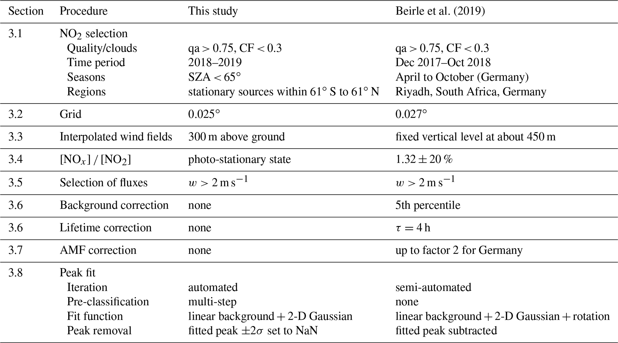
In this section we describe the data processing step by step. Table 1 summarizes the main steps and also lists similarities and differences to the procedure described in Beirle et al. (2019).
Beirle et al. (2019)Table 1Processing settings in this study as compared to Beirle et al. (2019).
3.1 NO2 selection
For this study, we select TROPOMI tropospheric NO2 column densities for the years 2018–2019 with values of the data quality indicator (“qa value”) above 0.75, as recommended in Geffen et al. (2019), and effective cloud fractions (CF) below 0.3. These selection criteria are the same as in Beirle et al. (2019).
In addition, we skip measurements with solar zenith angle (SZA) above 65∘ for the calculation of fluxes. This strict criterion removes observations for sun being low and implicitly results in a gradual removal of wintertime measurements for midlatitudes, while in Beirle et al. (2019), winter months have been skipped explicitly for Germany. Wintertime measurements are skipped in order to avoid unfavorable viewing conditions, snow-covered scenes, and stronger interference with aged plumes due to longer lifetimes. Moreover, the SZA restriction allows us to simply parameterize the NO2 photolysis as a function of the SZA (see Sect. 3.4).
Since large parts of the globe are free from stationary NOx point sources, in particular oceans, deserts, and forests, the processing focuses on potentially stationary sources. For this purpose, a selection mask is defined (Fig. 1), which is based on magnitude as well as the temporal variability of TROPOMI NO2 TVCDs. The construction of the selection mask is explained in detail in the Supplement.
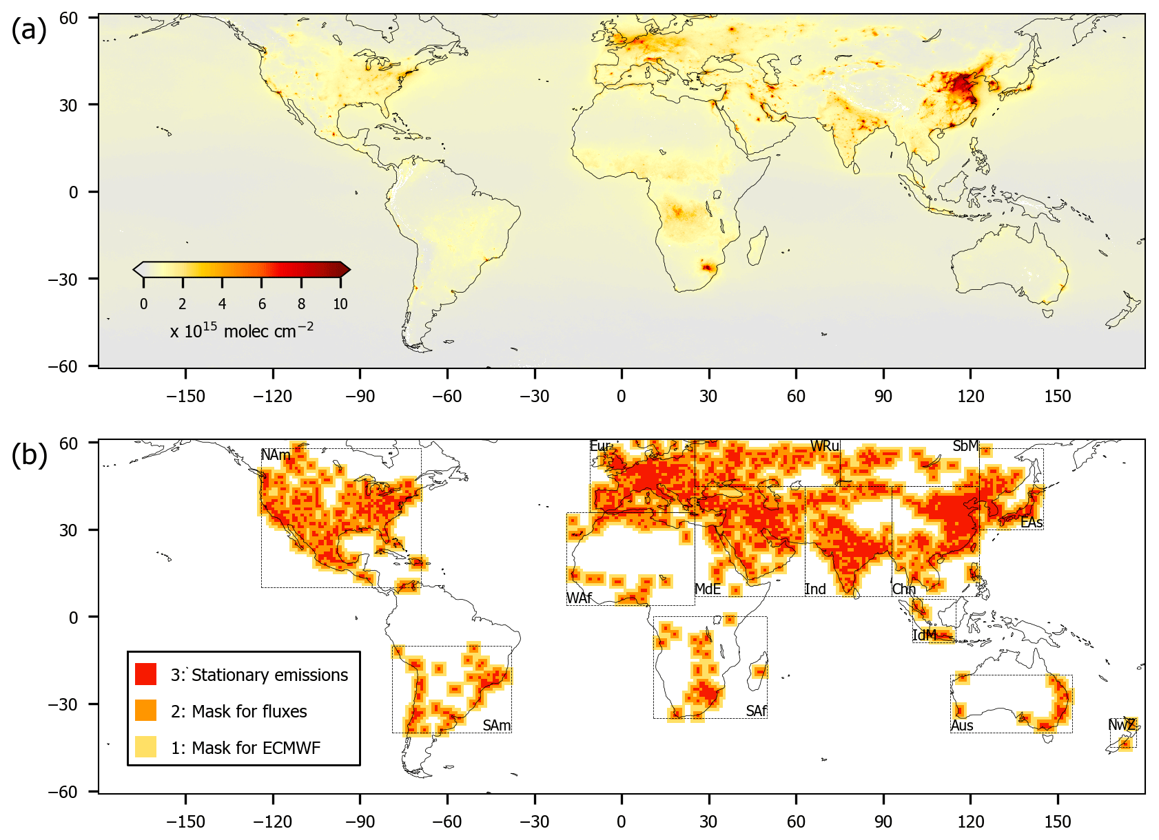
Figure 1(a) Mean tropospheric NO2 column density for 2019. (b) Mask M for the selection of pixels investigated in this study. The construction of M is described in the Supplement. Boxes indicate the regions as defined in Table 2.
3.2 Grid
In order to have maximum sensitivity for point sources, the TROPOMI observations have to be oversampled, requiring a fine grid resolution of less than 3 km. For each TROPOMI orbit, is thus gridded to a regular longitude/latitude grid with 0.025∘ resolution for 61∘ S to 61∘ N. Note that there are a few small NOx sources north of 61∘, but due to the strict SZA threshold of 65∘, the flux statistics would be poor for higher latitudes.
Gridding is done per orbit based on linear 2-D interpolation of TROPOMI pixel centers using the griddata function from the Python module SciPy (Virtanen et al., 2020). This approach allows for fast gridding. In addition, there are no discontinuities at the TROPOMI pixel borders, which would lead to extremely high (positive and negative) values of the derivative.
All missing values (qa < 0.75) as well as the outermost pixels on each side of the TROPOMI swath (i.e., the pixels with the highest viewing zenith angles) are set to not a number (NaN). This is necessary in order to restrict the area of interpolated TVCDs to the actual area covered by measurements.
Hereafter we denote the longitude and latitude dimensions as x and y, respectively, in vector indices as well as in the text.
3.3 Meteorological data
The meteorological datasets u, v, p, and T are extracted from ECMWF input data by linear interpolation in three steps:
-
In vertical dimension to an altitude of 300 m above ground for each ECMWF input dataset with 6-hourly resolution. As emissions from point sources are the focus of this study, we consider wind fields representative for the transport of freshly released NOx emissions from stacks. The choice of altitude of wind fields is further discussed in Sect. 5.2.3. Only pixels with the mask M ≥ 1 are extracted.
-
In time dimension to the orbit time stamp of each TROPOMI orbit, as given in the orbit filename. The actual TROPOMI overpass lags the orbit time stamp by about 33 and 67 min at 60∘ S and 60∘ N at solstice ±7 min for summer/winter. Thus the orbit time stamp reflects the wind conditions for recent plume histories.
-
In horizontal dimensions (latitude, longitude) to the 0.025∘ grid.
3.4 Upscaling of NO2 to NOx
In this study we scale the measured NO2 TVCD to a NOx TVCD for each TROPOMI pixel. The conversion factor L is calculated according to the photostationary steady state:
The impact of volatile organic compounds (VOCs) is neglected here as the focus is put on NOx point sources and thus generally high NOx concentrations.
The photolysis frequency of NO2 J is parameterized as a function of the SZA θ by
as proposed by Dickerson et al. (1982). This parameterization is “accurate to about 10 % for mostly sunny conditions” for SZA < 65∘ (Dickerson et al., 1982).
The reaction rate constant k for the reaction of NO with O3 is parameterized as a function of temperature (in kelvin) by
following the recommendations from Atkinson et al. (2004) and IUPAC (2013).
Near-surface ozone mixing ratios are taken from a climatology based on the ESCiMo model simulation (Sect. 2.3) and converted into concentrations based on T and p from ECMWF.
The derived values for L represent conditions for near-surface pollution. For background NOx in the upper troposphere, the partitioning would be shifted towards NO. However, any additive background is automatically removed by the calculation of the divergence. Thus, the partitioning derived for near-surface concentrations is appropriate also for correcting the added column caused by a point source.
Figure 2 displays the ratio of temporal means of NOx and NO2 TVCDs. Global mean is 1.35 with a SD of 0.08. Values for Riyadh, South Africa, and Germany are 1.22, 1.36, and 1.41, respectively, in agreement with the value of 1.32 ± 0.26 applied in Beirle et al. (2019), which was based on the number given in Seinfeld and Pandis (2006) for polluted conditions around noontime.
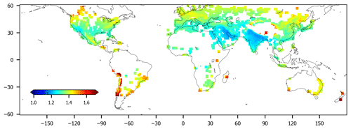
Figure 2Effective ratio, i.e., mean tropospheric NOx (as derived by assuming photostationary state according to Eq. 2 for each TROPOMI pixel) divided by the mean NO2 column density for 2018–2019. Note that only cloud-free observations with SZA < 65∘ are considered; thus wintertime measurements at mid- to high latitudes are skipped, and the expected latitudinal dependency of the ratio is suppressed. The spatial variability is a consequence of the dependency of the photostationary state on actinic flux, ozone concentration, and temperature (Eq. 2).
Note that the actual [NOx] [NO2] ratio close to a point source might be different in the case of high NO concentrations causing O3 titration. In this case, however, the divergence method would detect the emitted NOx downwind from the source as soon as the NO is converted to NO2 after mixing with ambient air. This results in a spatial smearing of the peak in the divergence map, leading to broader peaks, but the same integral (and thus emissions) for the peak fitting algorithm (Sect. 3.8.2). For the final budget of NOx emissions, which are determined from the integrated peaks, the final photostationary state is thus still adequate.
3.5 Gridded fluxes and divergence
From gridded NOx columns and gridded wind fields, the gridded NOx flux in both the x and y direction is derived for each TROPOMI orbit. Mean fluxes are calculated for the period 2018–2019, where calm wind conditions (w<2 m s−1) are skipped. For grid pixels with less than 25 measurements, fluxes are set to missing values due to poor statistics. Note that we do not explicitly skip winter months for midlatitudes, as in Beirle et al. (2019) for Germany, but they are removed implicitly by the strict SZA threshold of 65∘.
From the mean zonal and meridional flux maps, the divergence map is calculated, which is the basis for the identification and quantification of point sources below.
3.6 Lifetime and background corrections
In Beirle et al. (2019), emission maps were derived by adding the sink term to the divergence map. For this, a constant lifetime of τ=4 h was applied, as derived from OMI data for Riyadh (Beirle et al., 2011). In addition, V was corrected by subtracting the regional background, as the lifetime estimate was derived for freshly released, near-surface pollution, while upper-tropospheric background NO2 generally has a longer lifetime.
As discussed in Beirle et al. (2019), the inclusion of the sink term has significant impact on area sources; it contributes about 50 % of integrated emissions for the Riyadh urban area. For point sources, however, the emission signal is by far dominated by the divergence term, for instance accounting for 87 % of the emissions from power plant “PP9” in Beirle et al. (2019).
Within this study, we do not correct for the sink term S for the following reasons:
-
The NOx lifetime is expected to be different for the diverse conditions in the considered regions, covering a large variability of temperature, humidity, actinic flux, VOC levels, and NOx levels. Note that the expected strong dependency of mean lifetime on latitude is again suppressed here due to the selection of SZA < 65∘.
-
NOx lifetimes simulated from global models cannot resolve the nonlinearities caused by point sources. In addition, emission inventories used as input to model runs generally have a time lag; thus emissions are outdated for quickly developing countries. Consequently, modeling the NOx lifetime for the investigated point sources is challenging and uncertain.
-
Identifying point sources in the divergence map D directly is more immediate than in , as point sources reveal sharper peaks in D than in E (Fig. 2 in Beirle et al., 2019). In addition, the identification of ambiguous candidates as, e.g., caused by inaccurate wind fields is clearer based on D directly (Sect. 3.8.1).
The resulting low bias of point source emissions caused by the missing lifetime correction is discussed in Sect. 5.2.2.
Since no lifetime correction with is performed, also the background correction for V, which was performed in Beirle et al. (2019) in order to exclude upper-tropospheric NOx with longer lifetime and different L, is omitted in the current study. Note that the local background of V, as well as any potential offset due to, e.g., stratospheric correction, would affect the lifetime correction but have no impact on D, as any additive term is lost by the calculation of the derivative.
3.7 AMF correction
Tropospheric column densities of NO2 are derived from the total slant column by subtracting the stratospheric column and applying the so-called air mass factor (AMF). The AMF can be derived as the sum of height-dependent ”box AMFs”, representing the vertical measurement sensitivity, weighted by the relative profile (Wagner et al., 2007). In the operational TROPOMI NO2 product, averaging kernels (AKs) are provided that are proportional to box AMFs and allow us to correct the AMF for a different vertical profile (Eskes et al., 2003).
Validation studies report on a general low bias of NO2 TVCD from TROPOMI of a factor of 2 and more for polluted sites (e.g., Verhoelst et al., 2021; Judd et al., 2020), caused by a high biased AMF. Part of this bias seems to be related to the a priori profiles which do not resolve the pollution profiles close to sources. In addition, there are indications that the cloud heights used for the TVCD retrieval are biased low (Compernolle et al., 2021) and the albedo maps used are biased high (Griffin et al., 2019), resulting in biased AKs.
In Beirle et al. (2019), an AMF correction was performed for South Africa and Germany by applying the provided AK to a near-surface profile. In this study, we do not apply such an AMF correction, as the effects of biased input albedo and cloud height cannot be corrected a posteriori based on the provided AKs but require a reprocessing of the TROPOMI NO2 product.
Consequently, the low bias of TROPOMI TVCDs is directly transferred into the NOx emissions listed in the catalog, as discussed in detail in Sect. 5.2. The low bias is expected to be improved with an updated NO2 product, which will then be used for deriving an updated version of the point source catalog.
3.8 Iterative peak fitting
We apply a fully automated iterative peak fitting algorithm in order to detect NOx point sources. The goal is to identify clear point source peaks in the divergence map, where a robust quantification of emissions is possible, while ambiguous cases are skipped. Thus, the resulting catalog of point sources is incomplete; a detailed discussion on various reasons for missing point sources is given in Sect. 5.1. But the remaining point sources listed in the catalog correspond to actual NOx sources with high confidence.
In each iteration, the following procedure is executed:
-
The grid pixel with highest value of the divergence is considered the point source candidate.
-
Each candidate is classified into different categories and skipped if ambiguous (Sect. 3.8.1).
-
For a promising candidate, a 2-D Gaussian is fitted to the divergence peak, and successful fits are included in the catalog (Sect. 3.8.2).
-
The candidate is removed from the divergence map before searching for the next highest D value (Sect. 3.8.3).
The iteration stops as soon as the maximum value of the divergence is less than 0.2 µg m−2 s−1, which is <4 % of the initial maximum value of the first iteration. Below this threshold, almost no further point sources could be detected which meet the quality criteria listed below. For future versions, the availability of several years of TROPOMI data is expected to decrease the noise in divergence maps and will probably allow us to decrease this threshold and investigate additional small NOx point sources.
3.8.1 Pre-classification of candidates
Point source candidates are iteratively defined as the location of maximum divergence in the global map. Before fitting a Gaussian peak, and quantifying emissions, however, artifacts and ambiguous cases have to be excluded.
For this, a pre-classification is done based on the divergence map 30 km around the candidate. As soon as the candidate is classified as one of the following categories, the pre-classification stops. In Fig. 3, examples for each category are shown.
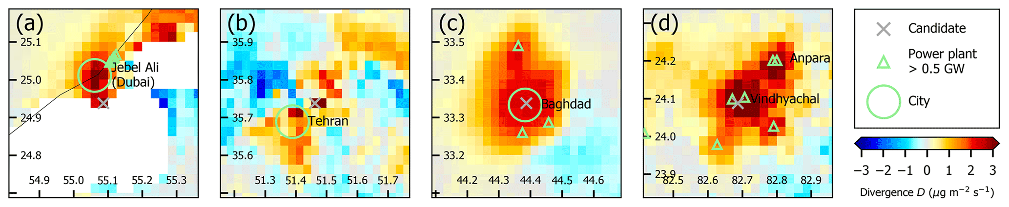
Figure 3Clippings of the mean divergence (2019–2020) showing examples for the different categories of point source candidates checked during pre-classification. White indicates missing data. The location of power plants from GPPD as well as cities is indicated by green markers. (a) “Gap” candidate near Jebel Ali/Dubai. (b) “Negative” candidate near Tehran. (c) “Area source” around Baghdad. (d) “Area source” candidate covering several power plants (with Vindhyachal and Anpara being the largest) in India.
-
Gap category. If more than 25 % of grid pixels are missing within 8 km around the candidate, it is classified as “gap”. Gaps were found primarily at sandy coastlines and are caused by persistent cloud coverage above threshold, which is probably an artifact of the coarse resolution of the albedo map used for the cloud retrieval. In the later stage of the iteration, gaps also occur in the vicinity of strong point sources which have been already removed from the divergence map. Figure 3a displays an example for a candidate of the gap category around Dubai, where the global maximum of divergence was found, but missing data do not allow for further quantifications.
-
Negative category. If the minimum divergence within 30 km is negative with an absolute value larger than 50 % of the maximum value, the candidate is “negative”.
Negative values of the divergence generally indicate NOx sinks. Thus values of D<0 have to be expected downwind from sources. But absolute values should be far lower than the positive values at the place of emissions, as the NOx removal is taking place over large distances (at a wind speed of 5 m s−1, a lifetime of 4 h corresponds to an e-folding distance of 72 km).
High absolute values of negative divergence thus cannot be explained by chemical loss of NOx (except for very short lifetimes) but indicate an inappropriate simplification of the complex 3-D wind fields by a 2-D wind vector on rather coarse spatial resolution. Also changes of NOx emissions or wind patterns on temporal scales of some hours (whereas Eq. 1 assumes steady state, i.e., neglects the temporal derivative of V) can cause high negative values of D.
Figure 3b displays an example of high negative divergence around Tehran. Obviously, the divergence method fails here, even though TVCDs show a hotspot of very high NO2 around Tehran that can even be spotted in the global map (Fig. 1a). The reason for the noisy divergence is the location of Tehran next to the Alborz mountains, where actual wind patterns are not described appropriately by the low-resolution wind fields.
-
Area source category. If the candidate is neither classified as “gap” nor as “negative”, sections of zonal and meridional means are calculated in order to allow for a quick check of the spatial extent of the divergence peak. For both sections, the full width at half maximum (FWHM) Wfirst guess is determined by checking for the first occurrence of a value below half of the maximum in both directions. For point sources, a FWHM of about 12 km has been reported in Beirle et al. (2019). Values of Wfirst guess above 17 km in both x and y thus indicate a NOx source, which cannot be categorized as single point source, but an area source, which could be a large city or an extended industrial area with several point sources nearby. Figure 3c and d display two examples for candidates classified as “area source”. Figure 3c shows the city of Baghdad. In Fig. 3d, an “area source” consisting of several point sources close to each other is shown, primarily the coal-fired power plants Vindhyachal (5 MW) and Anpara (2 MW) in India.
3.8.2 Gaussian fit
If a candidate passes all pre-classification checks, a 2-D Gaussian on top of a linear background is fitted to the peak in the divergence map:
with the fit parameters A being the peak integral; σx and σy being the width of the Gaussian; Δx and Δy being the shift of the peak maximum (relative to the first guess candidate location corresponding to the highest D value); and mx, my, and b describing a linear background.
In contrast to Beirle et al. (2019), no rotation of the peak is allowed in order to make the fit fast and stable and in order to be able to interpret the widths σx,y as actual distance in latitudinal and longitudinal dimensions.
The parameters are determined by a least-squares fit of G to the divergence map within 22 km around the candidate. As starting values, σx,y are set to Wfirst guess/2.355 for both x and y. But since the fit yields a more robust measure of the peak width than the simple FWHM estimate determined during pre-classification, the candidate is again classified as “area source”, if exceeds 17 km for x or y.
Otherwise, the candidate is considered to be a point source, where the fitted parameter A of the Gaussian peak represents the corresponding point source emissions. However, in order to only keep robust emission estimates in the point source catalog, cases with emissions below 0.03 kg s−1 (which has been derived in Beirle et al., 2019 as the detection limit for optimal conditions) or a relative fit error above 30 % are categorized as “uncertain”.
3.8.3 Candidate removal
The candidate has to be removed from the global map before the next iteration step. Removal is implemented by setting the divergence values around the maximum to NaN. Note that in Beirle et al. (2019) the fitted peaks were subtracted instead. However, this would introduce a highly structured residue in the divergence map, which would create several new artificial candidates for the fully automated peak search algorithm. Removing candidates by setting D to NaN avoids such artificial point sources and prevents any later interferences from fit residues from neighboring sources.
Depending on the classification, the following procedure is applied:
-
For point sources, an ellipse with 2 as a semi-major/minor axis is removed, with σx,y from the Gaussian fit.
-
For categories “gaps” and “uncertain”, all pixels within 22 km around the maximum are removed.
-
For category “negative”, a larger area (30 km around the maximum) is removed, as negative artifacts generally occur not at but next to the sources.
-
For area sources, also an area of 30 km around the maximum is removed, if classified based on Wfirst guess. If the area source was classified based on Wfit, an ellipse with 2 is removed as for point sources.
3.9 Identification of point sources associated with power plants
We perform an automated match of the point source catalog with the combustion power plants listed in GPPD. For each point source, we search for GPPD entries within 5 km radius. In the point source catalog, we add
-
the integrated capacity of all power plants within 5 km,
-
a complete list of the names of all power plants within 5 km, and
-
the primary fuel of the power plant with highest capacity within 5 km.
4.1 Candidate classification
The iterative peak fitting algorithm yields 7250 candidates, of which 451 are classified as point sources. For 242 of these point sources, a match with GPPD power plants was found. Table 3 lists the classification statistics for the regions defined in Table 2.
Table 2Definition of regions used for the regional statistics shown in Table 3 and for regional figures shown in the Supplement.
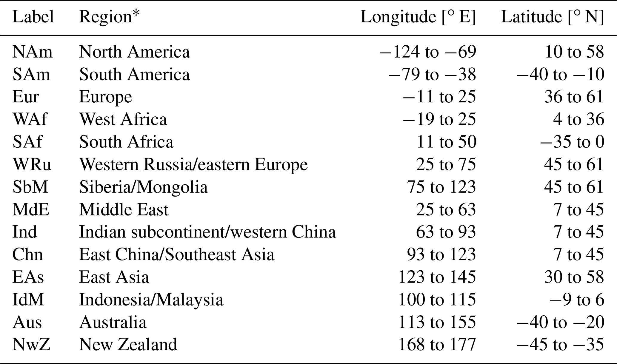
* Note that the regions are defined such that all considered pixels are covered by a limited number of figures with similar area as far as feasible. Region names are mostly based on continents. For Asia, regions are labeled after the countries dominating the detected point sources, gaining tangibility while condoning some inaccuracies in actual country borders.
Table 3Number of candidates and their respective classification found for the regions defined in Table 2. The number of point sources in brackets refers to the point sources associated with power plants.
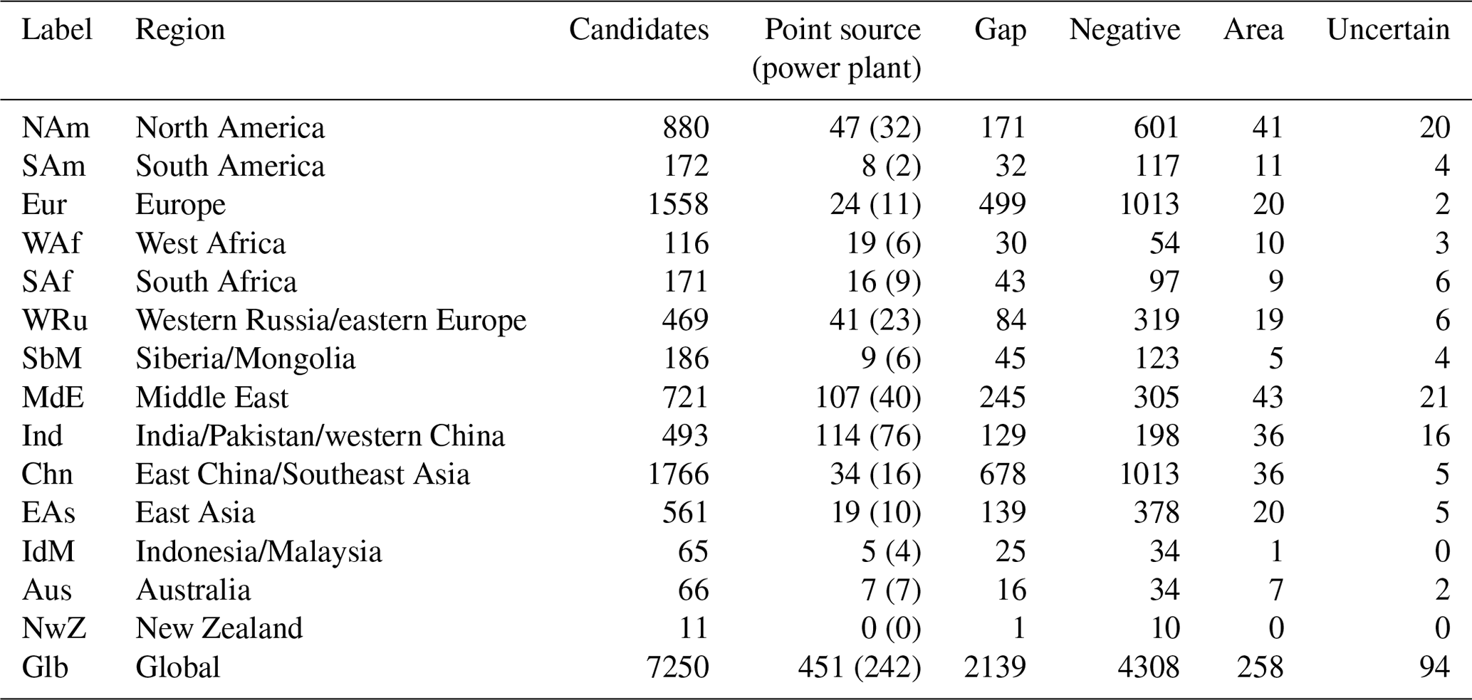
Figure 4 displays regional maps of color-coded D for selected regions. The respective maps for all regions listed in table 2 are provided in the Supplement in PDF format, allowing for loss-free zooming.
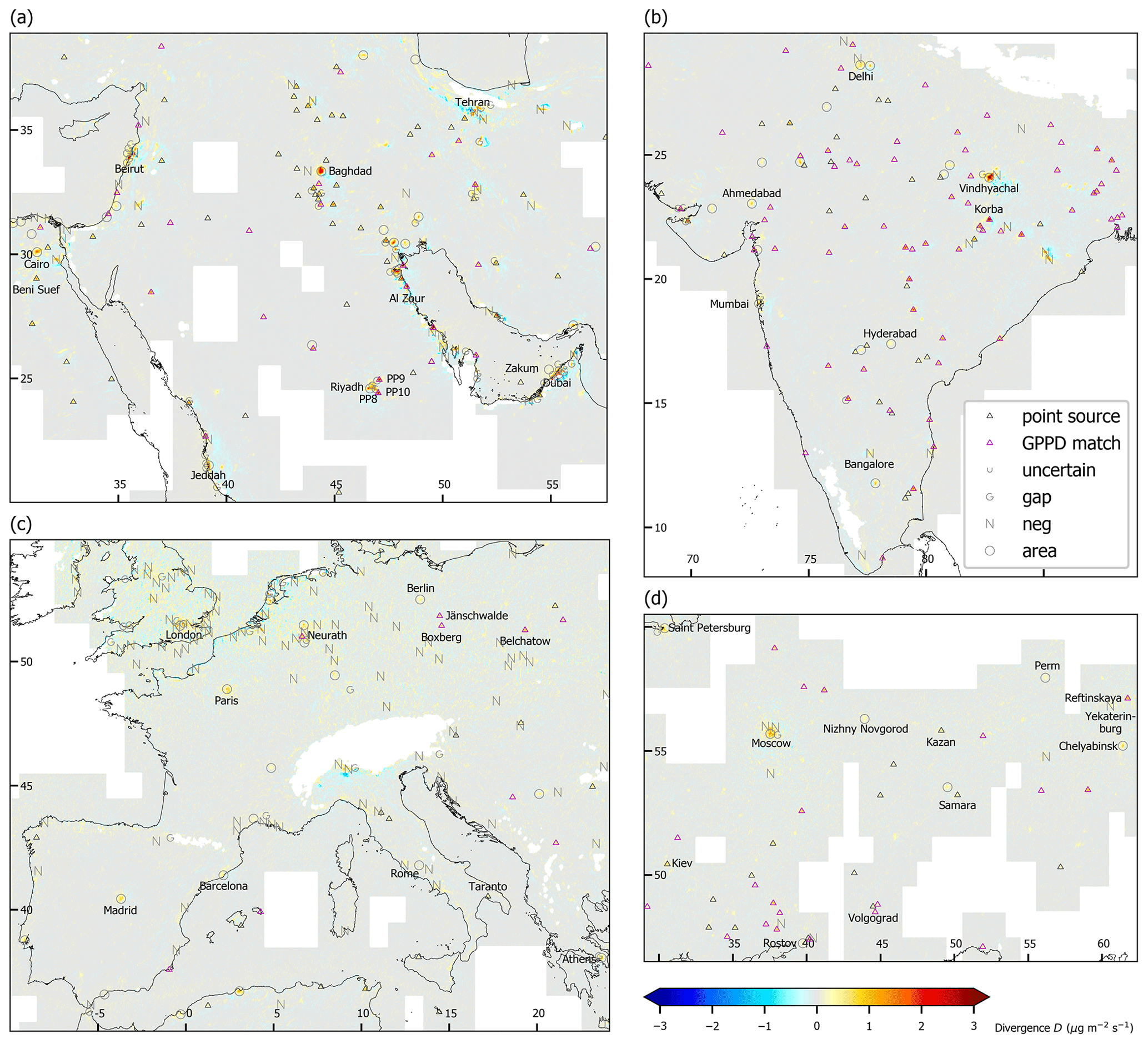
Figure 4Divergence D (color coded) and point source classification (symbols) for (a) the Middle East, (b) India, (c) Europe, and (d) Ukraine/western Russia. Triangles display the point sources listed in the catalog, where matches to GPPD power plants are indicated in magenta. Respective maps for all regions defined in Table 2 are provided in the Supplement (Figs. S2–S14). Also for sake of clarity, non-point sources are only shown for candidates with Dmax>1 µg m−2 s−1 or the integrated divergence within 30 km exceeding 0.1 kg s−1.
The candidate classifications are indicated by symbols, where point sources with/without a power plant match are displayed as triangles in magenta/dark grey, respectively. Non-point sources are shown in light grey. For sake of clarity, they are only displayed for high divergence values (Dmax>1µg m−2 s−1 or integrated D>0.1 kg s−1), as they would otherwise dominate the figure for some regions like Europe, where 499 candidates are classified as “gap” and 1013 as “negative” (Table 3).
The map of the Middle East (a) contains most of the non-point-source examples shown in Fig. 3. Several more gaps occur all along the Persian Gulf coastline, and further negative candidates are found in mountains as well as along the coastlines.
Several large cities like (a) Cairo and Jeddah, (b) Paris and Madrid, (c) Delhi and Mumbai, or (d) Moscow and Saint Petersburg are categorized as area source. However, there are also some candidates categorized as area source which do not correspond to a megacity. In particular the candidate corresponding to the maximum divergence over India, which is caused by the coal-fired 5 GW Vindhyachal Super Thermal Power Station, was categorized as area source, as it interferes with the 4 GW Anpara power plant about 16 km northeast (Fig. 3d). Such sources could still be investigated in detail based on the divergence map. However, for interfering sources so close to each other, a quantification by a fully automated algorithm is challenging.
For Riyadh, the power plants PP9 and PP10 northeast and southeast of the city center are identified as point sources (compare Beirle et al., 2019). In contrast to Beirle et al. (2019), PP8 west of Riyadh is not identified as a point source as it could not be separated from Riyadh city, as a consequence of the strict pre-selection of candidates and the slightly larger fit interval, which were necessary in order to run the algorithm fully automated globally.
Several point sources are detected in the Middle East. There is a remarkable cluster of several point sources detected south of Baghdad. Note that there was even a point source detected within the Persian Gulf, which corresponds to the Zakum offshore oilfield.
The Indian subcontinent reveals the highest number of point sources of the investigated regions, contributing one-fourth of the global number. This reflects the quickly growing industrial activities, while measures for emission reduction still need to catch up. In addition, the divergence method obviously works very well for India, as the noise in divergence is quite low. This might be related to the dry season providing very good observation conditions without gaps, thereby suppressing sampling effects (compare Sect. 5.1.1).
In Europe, only very few point sources are detected, like the world's largest charcoal power plant Bełchatów in Poland; the German charcoal power plants Jänschwalde, Boxberg, and Neurath/Niederaußem (compare Beirle et al., 2019); or Europe's largest steel plant in Taranto, southern Italy. Remarkably, almost no point sources are detected for England and the Benelux countries, where the mean TVCD has a local maximum (Fig. 1a). Instead, there are several candidates classified as “gaps” and “negative”, which is related to the high noise observed in the divergence map. A similar situation is found for China, where TVCD is highest globally (Fig. 1a), but noise in D is large (Fig. S11 in the Supplement) such that the number of negative candidates is high (1013), but only few (34) point sources could be clearly identified. In Ukraine and western Russia, where mean TVCD levels are moderate, several point sources could be clearly identified. These striking regional differences in the performance of the automated point source detection will be discussed in detail in Sect. 5.1.
4.2 Catalog of point sources
We derive a global catalog of NOx emissions from the 451 peaks categorized as point sources by sorting them according to the fitted emissions. A complete list of all detected point sources, including latitude/longitude and the estimated emissions, is provided in CSV format at https://doi.org/10.26050/WDCC/Quant_NOx_TROPOMI (Beirle et al., 2020) and also added as a data file to the Supplement.
Table 4 lists a selection of the identified point sources with some additional information on the respective NOx source. It contains the top 10 emitters of the catalog. In addition, every 100th rank is included in order to illustrate conditions for lower divergence levels. Divergence maps for the same selection are shown in Fig. 5, where also external information on NOx sources have been added. In the Supplement, respective divergence maps and tables of regional top emitters are shown for all considered regions.
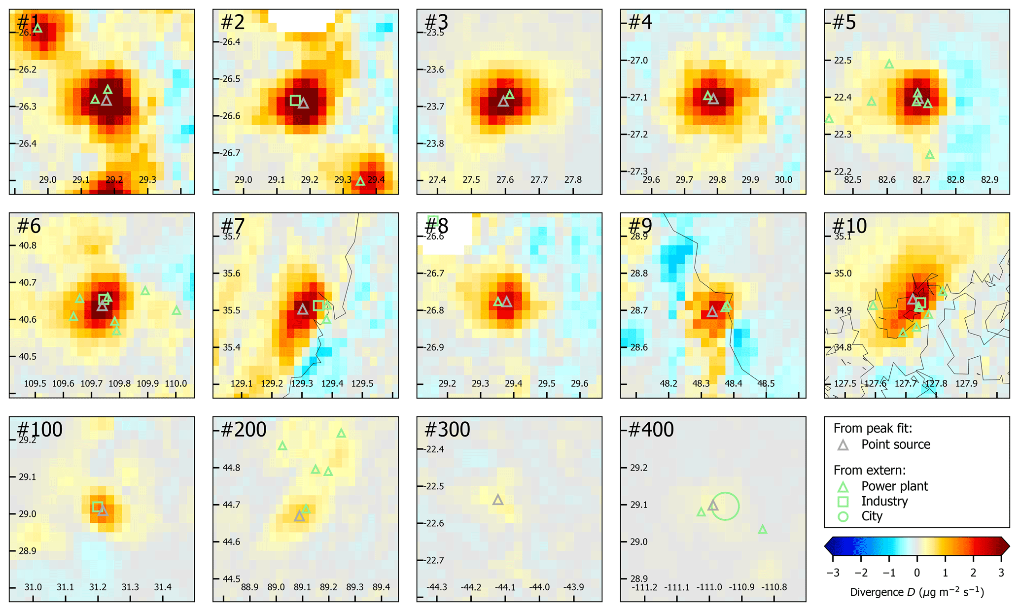
Figure 5Divergence maps for the selected point sources listed in Table 4. In addition to the location of the fitted Gaussian peak (grey), also some external information on GPPD power plants as well as industrial facilities and cities is added (green).
Most of the point sources listed in Table 4 can actually be associated with single or groups of power plants. Overall, a GPPD match was found for 242 point sources. The median distance between GPPD and point source locations was found to be 1.6 km, which is better than TROPOMI resolution. For the selection in Table 4, we did some additional inquiry and could identify the power plants Medupi (no. 3) and Presidente Vargas (no. 300), both missing in GPPD, as probable NOx sources.
Table 4Extract of the point source catalog for the top 10 and every 100th rank. Power plant capacity, fuel type, and facility names are added for matches to GPPD. The last two columns are not part of the catalog but have been added manually for the presented selection in order to provide information on the likely NOx source where no (or insignificant) GPPD match has been found. Divergence maps for the same selection are displayed in Fig. 5. As discussed in detail in Sect. 5.2.6, the given emissions are biased low. Respective tables for regional top emitters are listed in the Supplement for all considered regions.

1 Primary fuel of the GPPD match with highest capacity within 5 km.
2 GPPD names have been shortened.
3 Missing in GPPD.
Other point sources are the Secunda CTL coal liquifying facility (no. 2), steel work facilities (no. 6, no. 10), and a cement plant (no. 100). Point source no. 7 is located in Ulsan, an industrial hotspot in South Korea. Here, however, we could not identify a single dominating NOx point source. For the Hermosillo power plant, the peak fit is probably affected by Hermosillo city nearby (0.7 million inhabitants).
The four highest point source NOx emissions are all found for South African coal power plants, which have already been presented in Beirle et al. (2019). Note that the emissions in Table 4 are lower than those given in Beirle et al. (2019) for various reasons, as discussed in detail in Sect. 5.2.6, mainly due to the missing AMF and lifetime corrections in the current study.
The thresholds for artifacts in divergence have been defined rather strictly. Consequently, the remaining locations listed in the catalog actually indicate stationary NOx emissions. In the spot tests investigated exemplarily, we found no indication for false signals in the catalog.
4.3 Comparison to power plant database
Figure 6a provides a scatter plot of power plant capacity and point source emissions. Respective regional figures for all considered regions are provided in Fig. S15 in the Supplement.
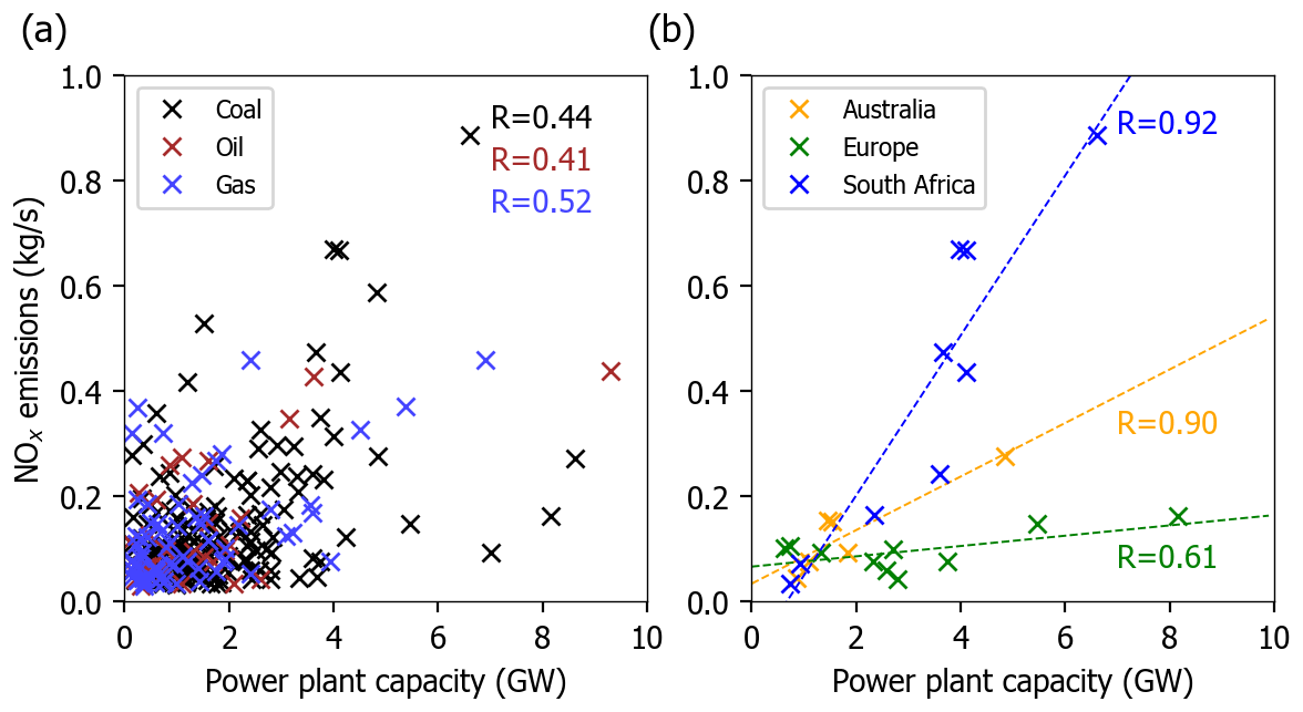
Figure 6Correlation between point source emissions and power plant capacity. (a) Scatter plot for all matches globally, with color coding primary fuel. (b) Scatter plot for coal-fired power plants in Australia, Europe, and South Africa.
Note that a perfect correlation between power plant capacity and NOx emissions cannot be expected, as the emissions per capacity strongly depend on fuel type and technology and are particularly modified if emission control measures like selective catalytic reduction (SCR) are applied. High emissions for power plants with low capacity probably indicate other dominating NOx sources nearby, like for Baotou (no. 6), where a 0.2 GW power plant was matching the point source location, but emissions are probably mainly caused by the metal smelting facilities. Low emissions from high-capacity power plants probably indicate the installation of SCR or a recent reduction in capacity.
High correlations can be observed for some regions like South Africa and Australia. This is probably indicating that the GPPD entries are reliable for these regions, the level of power plant technology is regionally similar, and the divergence method works well here. Figure 6b displays the scatter plots for coal-fired power plants for Australia, Europe, and South Africa. The slopes indicate clear regional differences in the emissions-per-capacity ratio.
In this section we discuss the limitations as well as the potential of the presented point source catalog, give an outline on possible applications, and an outlook on improvements of the catalog in a future update.
5.1 Limitations
When interpreting the presented point source catalog, the following limitations have to be kept in mind.
5.1.1 Missing point sources
The catalog is incomplete, as point sources might be missing due to the following reasons:
-
Considered pixels. Only latitudes between 61∘ N/S are considered, as for higher latitudes, the strict SZA threshold of 65∘ would result in poor statistics. In addition, the criteria for defining the selection mask are quite strict in order to reduce the amount of data to be processed. There might thus be NOx point sources not included in the selection mask. However, based on maps of the mean TVCD, we see no indication for strong point sources outside the considered area defined by M (compare Fig. 1a and b).
-
Gaps in input data. The mean divergence map reveals persistent gaps at some coastlines, in particular around the Persian Gulf. These gaps are caused by the cloud algorithm, as cloud retrievals are challenging for the transition of dark ocean to bright sand. The situation will improve for an updated cloud product which will be based on a ground albedo with higher spatial resolution.
-
Artifacts in divergence. In cases of inaccurate wind fields, as over mountainous terrain, as well as for systematic violation of the steady-state assumption, like systematic diurnal cycles of wind direction, the divergence map reveals artifacts, i.e., patterns of high negative values for D which cannot be explained by the loss term S. These cases are classified as “negative” and are thus missing in the catalog.
-
Noise in divergence. The noise level of the divergence map reveals large regional differences, causing respective differences in the performance of the peak fit algorithm. Noise levels are particularly high over regions with generally high TVCD levels, like eastern China or western Europe. This is caused by sampling effects. For high TVCD levels, also fluxes are generally high. As the daily flux maps have gaps due to cloud masking, the mean fluxes reveal “jumps”. This effect is probably intensified by the gridding by interpolation, where a gap (= missing value) in the input data results in gaps for a substantially larger area in the gridded data, as interpolation requires information from all surrounding pixels. Note that due to day-to-day changes of wind directions, a far higher amount of data would be needed in order to get smooth flux maps than to overcome the respective sampling issues in mean TVCDs. As the spatial derivative amplifies these jumps, the divergence is generally noisy over regions with high TVCD. Consequently, only few point sources are identified for the highly polluted regions in western Europe or eastern China, while many candidates are classified as “negative” due to the high noise levels.
-
Interfering sources. Point sources cause peaks in the divergence map which can be described by a Gaussian. Typical widths are km, in accordance to the spatial resolution of TROPOMI. Thus, point sources within a distance of less than about 20 km cannot be clearly separated by the automated algorithm. In cases of point sources close to each other, they are identified and quantified as one single point source (see next section), and their emissions are just added. If the distance is about 15–20 km, however, the joined peak from both sources is still processed as a single candidate but classified as “area source” due to the large width of the peak. For example, the Indian power plants Vindhyachal and Anpara located within 16 km (Fig. 3d) or PP8 at the western edge of Riyadh megacity (compare Fig. 2 in Beirle et al., 2019) are classified as “area source” and thus missing in the catalog.
5.1.2 Multiple sources
Due to the spatial resolution of TROPOMI, sources within about 10 km cannot be separated by the automatic peak-finding algorithm, and power plant stack emissions would automatically be merged with emissions from on-site activities such as heavy-duty diesel around the power plant. Several entries in the catalog contain multiple sources, like no. 1 (power plants Matla and Kriel within 5 km) or no. 3 (power plants Matimba and Medupi within 7 km). Similarly, the emissions from large industrial complexes, like the Ulsan industrial area, cannot be further specified. Thus the term “point source” means with respect to the TROPOMI spatial resolution. This is however still better resolved than many bottom-up inventories and typical horizontal resolutions of regional chemical transport models (CTMs). Thus, for emission inventories, also multiple and extended sources could appropriately be treated as point source emissions if used for models with a spatial resolution coarser than that of TROPOMI.
5.2 Uncertainties and accuracy
The main goal of v1.0 of the point source catalog is the identification rather than the quantification of NOx point sources. Still we discuss and try to quantify the various sources for uncertainties of the derived point source emissions.
5.2.1 Gridding
Gridding is done by 2-D linear interpolation, which avoids abrupt jumps at the satellite pixel edges. Such jumps would cause large response in the divergence, i.e., the spatial derivative.
For narrow plumes, however, linear interpolation carries the risk of introducing a low bias. We have investigated this exemplarily for the power plant plume of PP9 northeast of Riyadh on 17 December 2017 (Beirle et al., 2019, Fig. 1a therein). The average plume TVCD from interpolation yields almost the same value as for conventional gridding (1 % lower). For the peak maximum, however, which is more relevant for the divergence than the mean, interpolation is 6 % lower. Thus, there is a low bias caused by linear interpolation, which is small compared to the other effects discussed below.
5.2.2 Lifetime
The quantification of NOx emissions is based on the peak in D, ignoring the chemical loss of NOx during downwind transport. We estimate the impact of neglecting the lifetime correction by comparing the catalog emissions to the respective emissions based on E (assuming a lifetime of 4 h). On average, the latter were higher than those based on D by about 25 %, which is quite small compared to other effects, in particular the AMF (see below).
In cases of much shorter lifetimes, like 1.5 h, as reported by Goldberg et al. (2019) for the Colstrip power plant in the USA (Fig. 1 therein), the emission estimates after lifetime correction would be higher by a factor of 1.73 on average.
5.2.3 Wind fields
As discussed in Beirle et al. (2019), different effects on wind field uncertainties have to be considered:
-
Errors of the wind direction (both random and systematic) result in a underestimation of the flux and thus the estimated emissions, as any mismatch in wind direction leads to a low bias of the wind speed component projected to the actual wind direction. The underestimation is thus proportional to the cosine of the wind direction. For wind direction errors of 25∘, it is about 10 %.
Larger systematic errors in wind direction would cause visible artifacts in the divergence map and would thus be captured and removed by the check for negative divergence during candidate classification. In cases of larger random effects, the artifacts of individual days would at least partly cancel in the mean flux. But the wind speed component in the actual wind direction would be significantly underestimated, as well as the resulting divergence.
-
The calculated fluxes, and thus the divergence map, are proportional to wind speed. The choice of the altitude of input wind fields thus affects the resulting emissions, as wind speeds are generally higher for higher altitudes. In Beirle et al. (2019), the effect for taking wind fields from 250 or 730 m rather than from 450 m on emissions was quantified as about 10 %.
In this study, the focus was set to the clear identification of point sources. Thus, winds from a lower altitude (300 m) compared to Beirle et al. (2019) (450 m) were chosen in order to have optimal wind direction data close to the NOx emission source. As discussed below, this choice removes the artifacts of divergence around the Matimba/Medupi power plants seen in Beirle et al. (2019).
5.2.4 Peak fit
The fitted emissions depend on the settings for fit radius and the forward model function. The fit window of 22 km around the source was chosen as compromise in order to cover the peak caused by a point source as far as possible while avoiding interference with neighboring sources. Variations of the fit settings within reasonable limits cause an uncertainty of about 20 % in the fitted emissions (Beirle et al., 2019).
5.2.5 AMF
Validation studies report on NO2 TVCDs from TROPOMI being biased low for polluted sites (Verhoelst et al., 2021). This is probably due to the a priori vertical profiles, the cloud height product being biased low (Compernolle et al., 2021), and the surface albedo being biased high (Griffin et al., 2019), all resulting in high biased AMFs.
In Beirle et al. (2019), a correction of the low bias was applied by assuming the NOx profile close to point sources to be in the lowest layer. Note that since the divergence is sensitive for the change of the NOx flux due to the point source emissions, the required AMF correction has to be applied to the profile of the added rather than the total NOx.
Still, we do not apply such a correction here, since there are indications that the cloud heights and surface albedo used for the NO2 retrieval are systematically biased. Thus, also the provided AKs are biased, and a simple a posteriori correction of TVCDs is not possible.
For Germany, the AMF correction applied in Beirle et al. (2019) was a factor of 2 due to profile shape. In combination with a bias in the cloud height and ground albedo used for the TVCD retrieval, even higher factors have to be expected. The actual number will depend on surface albedo, aerosols, and cloud statistics (within the selection of low effective cloud fractions) and is high over dark surfaces and frequent cloud contamination but low over bright surfaces and few clouds (like for Riyadh). For partly clouded scenes, the AMF for the added NO2 column could be easily too high by an order of magnitude if the real cloud is above the plume, but the retrieved cloud is below. Consequently, the added NO2 would be biased low by an order of magnitude. This issue was improved in a recent update of the TROPOMI NO2 L2 processor now using improved albedo and cloud products and thus more appropriate AKs. However, so far, no reprocessed NO2 time series is available.
5.2.6 Low bias
As listed above, many effects contribute to the uncertainty of emission estimates from the divergence of mean NO2 fluxes. Several of these effects are systematic in nature, resulting in an overall low bias of the derived emissions. In particular the effects of biased cloud height and inaccurate a priori profiles are expected to reveal large regional dependencies. Consequently, the low bias is hard to quantify for the global catalog. Thus we decided not to try to correct for the low bias of catalog emissions in this study but present the low biased estimates as they are with a clear disclaimer that the given emission estimates are biased low.
Accordingly, the emission estimates for South Africa reported in Beirle et al. (2019) were higher than the values listed in Table 4 by a factor of about 1.87 (for Matla/Kriel) up to 2.56 (for Medupi/Matimba). This discrepancy is a consequence of the missing AMF correction (factor 1.35 applied in Beirle et al., 2019), the missing lifetime correction (factor 1.1), the wind input data from lower altitudes (factor 1.1), and differences in grid definition, fit function (no rotation), and fit settings (factor 1.2), which together explain a factor of 1.9 as found for Matla/Kriel.
For Medupi/Matimba, the reason for the remaining discrepancy is the difference in input wind fields. The winds from higher altitudes (450 m) used in Beirle et al. (2019) cause a pattern of high negative D southwest of the power plants, indicating a mismatch of wind direction (see Fig. S2B in the Supplement of Beirle et al., 2019). Even in E, after applying lifetime correction, the negative values southwest remain in maps of E (Fig. 4A in Beirle et al., 2019). Consequently, the fit function finds a low background with a linear increase from southwest to northeast, and the emissions fitted on top of this low background are biased high.
In the current study, this artifact is not present (see point source no. 3 in Fig. 5), indicating that the wind direction from lower altitude (300 m) matches better to the actual NOx transport of Medupi/Matimba emissions.
In the Supplement, catalog emissions are exemplarily compared to emissions reported by EPA for the top 10 emitters of the USA. A total of 7 of these 10 emitters are listed in the catalog, with correct naming found from the merging of GPPD. The other 3 emitters were also found as candidates but were classified as “negative”. EPA emissions were found to be higher than the emissions listed in the catalog by a factor of 3 (Navajo) up to 8 (Hunter). These power plants, however, are quite remote from large cities. Thus, in the absence of other significant NOx sources, the modeled profiles used as a priori for the calculation of AMFs do not reflect the near-surface power plant plume due to the coarse model resolution. In addition, the cloud altitude used for the calculation of averaging kernels is biased low (Compernolle et al., 2021), causing high biased AMFs and low biased columns. The impact of this bias can easily reach 1 order of magnitude for cases where the retrieval assumes a cloud below the plume, while it is actually above. For these reasons, we have to expect that the low bias of the partial column added by a point source close to the ground is considerably larger than that of the complete tropospheric column, where validation studies report typical low biases of a factor of 2 for polluted sites. We will focus on this issue more quantitatively when preparing an update of the catalog, which we plan to process after reprocessing of the TROPOMI NO2 product based on improved albedo and cloud products and thus more appropriate AKs.
5.3 Potential
Though the catalog is incomplete and the derived emissions are biased low, it still has the potential to improve our knowledge on NOx emissions. Here we discuss the benefits of the divergence approach and the point source catalog and propose future applications.
5.3.1 Localization of NOx and CO2 sources
The Gaussian fit determines the location of the peak maximum. For all catalog locations which were inspected manually (i.e., all point sources listed in Table 4 or labeled in Fig. 4), Google Maps quickly reveals a plausible origin of the emissions close to the fitted peak location. For the examples shown in Fig. 5 which are related to power plants, the fitted point source location agrees to the actual power plant locations within about 2–3 km. Thus, the point source catalog accurately lists the location of NOx point sources. As these sources are all related to combustion, this also provides valuable information on the location of CO2 sources, which may also help to quantify CO2 emissions from NO2 measurements (Liu et al., 2020) and current and future satellite measurements of CO2.
5.3.2 Spatial patterns
Within a regional focus, the catalog reflects the spatial distribution and relative importance of point sources. Regionally, high correlation between NOx emissions and power plant capacity was observed (Fig. 6). Thus, it might be possible to re-distribute emissions from bottom-up inventories regionally according to the location of point sources in the catalog.
In addition, striking discrepancies between bottom-up inventories and the catalog, like strong point sources present in one but missing in the other, might be investigated in more detail and should result in improved emission inventories.
5.3.3 Up to dateness
Bottom-up inventories based on fuel consumption statistics have to collect and process input data from national reports. Thus, they have a time lag and are outdated when released for countries with high dynamics in industrial activities. Based on the divergence of NO2 fluxes, single power plants can be identified and quantified, e.g., on an annual basis. This would allow us to detect short-term trends and power plants being switched on or off even in the vicinity of polluted cities such as Riyadh.
5.4 Outlook
This paper describes v1.0 of the NOx point source catalog. We plan to update the catalog as soon as a reprocessed TROPOMI NO2 product is available. We expect that some of the persistent gaps along coastlines, e.g., around Dubai, can be closed in the future, as soon as the cloud information is based on high-resolution maps of the surface albedo, and thus NO2 TVCD becomes available there. In addition, improved surface albedo, cloud height, and a priori profiles are expected to improve the TVCD and (at least partly) remove the low bias.
In addition, we plan to use meteorological data from ERA-5 on higher spatial and temporal resolution. Currently, 6-hourly model output of ECMWF meteorological data was interpolated to a regular horizontal grid with a resolution of 1∘. Case studies will be performed in order to find out which is the best compromise between spatiotemporal sampling and processing time.
TROPOMI NO2 data are available via Copernicus Sentinel-5P (processed by ESA), 2018, TROPOMI Level 2 Nitrogen Dioxide tropospheric column products, Version 01, European Space Agency, https://doi.org/10.5270/S5P-s4ljg54 (European Space Agency, 2019). The full NOx point source catalog v1.0 is available at https://doi.org/10.26050/WDCC/Quant_NOx_TROPOMI (Beirle et al., 2020). The corresponding divergence maps are provided by the authors on request.
The high spatial resolution provided by TROPOMI allows for the detection and quantification of strong NOx point sources like large power plants, metal smelters, cement plants, or industrial areas. We present v1.0 of a global catalog of NOx point sources derived from the divergence of the mean NO2 flux 2018–2019 by a fully automated iterative algorithm, yielding 451 point sources. A total of 242 of these point sources could be matched to combustion power plants from a global database, with a median distance of 1.6 km. The top four point source emissions are all located in South Africa and related to coal burning. About one-fourth of all point sources were found over the Indian subcontinent, where the method works quite well due to low noise levels.
The catalog is incomplete and misses point sources due to gaps in the divergence map (caused by gaps in the cloud product), artifacts in the divergence map (caused by non-steady state and inaccurate wind fields), noise in the divergence map (caused by sampling effects for regions with high background TVCD like western Europe or China), and interference of sources within about 10–20 km distance.
The listed emissions are biased low mainly due to a low bias of input TVCDs from TROPOMI. As this bias is expected to vary regionally and is hard to quantify, it is not corrected for v1.0 of the catalog. Exemplary comparisons to emissions reported from in situ monitoring reveals a low bias which can be as high as a factor of 8 for some power plants, which is probably caused by inappropriate a priori profiles and a low bias in the cloud height.
Still, the catalog has high potential for checking and improving emission inventories, as it localizes NOx (and also CO2) sources, provides spatial patterns of the distribution of sources, and yields up-to-date emission data.
The supplement related to this article is available online at: https://doi.org/10.5194/essd-13-2995-2021-supplement.
SB performed the analysis and wrote the paper with input from all co-authors. CB processed the TROPOMI L2 data. SD processed ECMWF meteorological data. HE performed the retrieval of operational TROPOMI L2 NO2 TVCDs. VK compiled the ozone climatology from ESCiMo model data. AdL initiated the matching between catalog point sources and GPPD. TW contributed to the data analysis and interpretation and supervised the study.
The authors declare that they have no conflict of interest.
Publisher’s note: Copernicus Publications remains neutral with regard to jurisdictional claims in published maps and institutional affiliations.
We thank ESA and the TROPOMI L1/L2 teams for realizing TROPOMI and providing NO2 tropospheric data. ERA-Interim and ERA-5 data used in this study are provided by the European Centre for Medium-Range Weather Forecasts (ECMWF). Andrea Pozzer is acknowledged for providing the ESCiMo model data used for the ozone climatology.
This paper was edited by Nellie Elguindi and reviewed by two anonymous referees.
Atkinson, R., Baulch, D. L., Cox, R. A., Crowley, J. N., Hampson, R. F., Hynes, R. G., Jenkin, M. E., Rossi, M. J., and Troe, J.: Evaluated kinetic and photochemical data for atmospheric chemistry: Volume I – gas phase reactions of Ox, HOx, NOx and SOx species, Atmos. Chem. Phys., 4, 1461–1738, https://doi.org/10.5194/acp-4-1461-2004, 2004. a
Beirle, S., Boersma, K. F., Platt, U., Lawrence, M. G., and Wagner, T.: Megacity Emissions and Lifetimes of Nitrogen Oxides Probed from Space, Science, 333, 1737–1739, https://doi.org/10.1126/science.1207824, 2011. a, b
Beirle, S., Borger, C., Dörner, S., Li, A., Hu, Z., Liu, F., Wang, Y., and Wagner, T.: Pinpointing nitrogen oxide emissions from space, Sci. Adv. 5, eaax9800, https://doi.org/10.1126/sciadv.aax9800, 2019. a, b, c, d, e, f, g, h, i, j, k, l, m, n, o, p, q, r, s, t, u, v, w, x, y, z, aa, ab, ac, ad, ae, af, ag, ah, ai, aj, ak, al, am
Beirle, S., Borger, C., Dörner, S., Eskes, H., Kumar, V., de Laat, A., and Wagner, T.: Quantification of NOx point sources from the TROPOspheric Monitoring Instrument (TROPOMI), World Data Center for Climate (WDCC) at DKRZ [data set], https://doi.org/10.26050/WDCC/Quant_NOx_TROPOMI, 2020. a, b, c
Bouarar, I., Brasseur, G., Petersen, K., Granier, C., Fan, Q., Wang, X., Wang, L., Ji, D., Liu, Z., Xie, Y., Gao, W., and Elguindi, N.: Influence of anthropogenic emission inventories on simulations of air quality in China during winter and summer 2010, Atmos. Environ., 198, 236–256, https://doi.org/10.1016/j.atmosenv.2018.10.043, 2019. a
Byers, L., Friedrich, J., Hennig, R., Kressig, A., Li, X., McCormick, C., and Malaguzzi Valeri, L.: A Global Database of Power Plants, World Resources Institute, Washington, DC, available at: https://datasets.wri.org/dataset/globalpowerplantdatabase (last access: 21 June 2021), 2019. a
Compernolle, S., Argyrouli, A., Lutz, R., Sneep, M., Lambert, J.-C., Fjæraa, A. M., Hubert, D., Keppens, A., Loyola, D., O'Connor, E., Romahn, F., Stammes, P., Verhoelst, T., and Wang, P.: Validation of the Sentinel-5 Precursor TROPOMI cloud data with Cloudnet, Aura OMI O2–O2, MODIS, and Suomi-NPP VIIRS, Atmos. Meas. Tech., 14, 2451–2476, https://doi.org/10.5194/amt-14-2451-2021, 2021. a, b, c
Dickerson, R. R., Stedman, D. H., and Delany, A. C.: Direct Measurements of ozone and Nitrogen Dioxide Photolysis Rates in the Troposphere, J. Geophys. Res., 87, 4933–4946, https://doi.org/10.1029/JC087iC07p04933, 1982. a, b
Eskes, H. J. and Boersma, K. F.: Averaging kernels for DOAS total-column satellite retrievals, Atmos. Chem. Phys., 3, 1285–1291, https://doi.org/10.5194/acp-3-1285-2003, 2003. a
European Space Agency (ESA): Copernicus Sentinel-5P data products, ESA [data set], https://doi.org/10.5270/S5P-s4ljg54, 2018. a
Goldberg, D. L., Lu, Z., Streets, D. G., de Foy, B., Griffin, D., McLinden, C. A., Lamsal, L. N., Krotkov, N. A., and Eskes, H.: Enhanced Capabilities of TROPOMI NO2: Estimating NOx from North American Cities and Power Plants, Environ. Sci. Technol., 53, 12594–12601, https://doi.org/10.1021/acs.est.9b04488, 2019. a
Griffin, D., Zhao, X., McLinden, C. A., Boersma, F., Bourassa, A., Dammers, E., Degenstein, D., Eskes, H., Fehr, L., Fioletov, V., Hayden, K., Kharol, S. K., Li, S.-M., Makar, P., Martin, R. V., Mihele, C., Mittermeier, R. L., Krotkov, N., Sneep, M., Lamsal, L. N., Linden, M. ter, Geffen, J. van, Veefkind, P., and Wolde, M.: High-Resolution Mapping of Nitrogen Dioxide With TROPOMI: First Results and Validation Over the Canadian Oil Sands, Geophys. Res. Lett., 46, 1049–1060, https://doi.org/10.1029/2018GL081095, 2019. a, b
Hoffmann, L., Günther, G., Li, D., Stein, O., Wu, X., Griessbach, S., Heng, Y., Konopka, P., Müller, R., Vogel, B., and Wright, J. S.: From ERA-Interim to ERA5: the considerable impact of ECMWF's next-generation reanalysis on Lagrangian transport simulations, Atmos. Chem. Phys., 19, 3097–3124, https://doi.org/10.5194/acp-19-3097-2019, 2019. a
IUPAC: Task Group on Atmospheric Chemical Kinetic Data Evaluation, available at: http://iupac.pole-ether.fr (last access: 21 June 2021), Data Sheet NOx24, last evaluated: June 2013. a
Jöckel, P., Kerkweg, A., Pozzer, A., Sander, R., Tost, H., Riede, H., Baumgaertner, A., Gromov, S., and Kern, B.: Development cycle 2 of the Modular Earth Submodel System (MESSy2), Geosci. Model Dev., 3, 717–752, https://doi.org/10.5194/gmd-3-717-2010, 2010. a
Jöckel, P., Tost, H., Pozzer, A., Kunze, M., Kirner, O., Brenninkmeijer, C. A. M., Brinkop, S., Cai, D. S., Dyroff, C., Eckstein, J., Frank, F., Garny, H., Gottschaldt, K.-D., Graf, P., Grewe, V., Kerkweg, A., Kern, B., Matthes, S., Mertens, M., Meul, S., Neumaier, M., Nützel, M., Oberländer-Hayn, S., Ruhnke, R., Runde, T., Sander, R., Scharffe, D., and Zahn, A.: Earth System Chemistry integrated Modelling (ESCiMo) with the Modular Earth Submodel System (MESSy) version 2.51, Geosci. Model Dev., 9, 1153–1200, https://doi.org/10.5194/gmd-9-1153-2016, 2016. a
Judd, L. M., Al-Saadi, J. A., Szykman, J. J., Valin, L. C., Janz, S. J., Kowalewski, M. G., Eskes, H. J., Veefkind, J. P., Cede, A., Mueller, M., Gebetsberger, M., Swap, R., Pierce, R. B., Nowlan, C. R., Abad, G. G., Nehrir, A., and Williams, D.: Evaluating Sentinel-5P TROPOMI tropospheric NO2 column densities with airborne and Pandora spectrometers near New York City and Long Island Sound, Atmos. Meas. Tech., 13, 6113–6140, https://doi.org/10.5194/amt-13-6113-2020, 2020. a
Leue, C., Wenig, M., Wagner, T., Klimm, O., Platt, U., and Jähne, B.: Quantitative analysis of NOx emissions from Global Ozone Monitoring Experiment satellite image sequences, J. Geophys. Res., 106, 5493–5505, 2001. a
Liu, F., Duncan, B. N., Krotkov, N. A., Lamsal, L. N., Beirle, S., Griffin, D., McLinden, C. A., Goldberg, D. L., and Lu, Z.: A methodology to constrain carbon dioxide emissions from coal-fired power plants using satellite observations of co-emitted nitrogen dioxide, Atmos. Chem. Phys., 20, 99–116, https://doi.org/10.5194/acp-20-99-2020, 2020. a
Lorente, A., Boersma, K. F., Eskes, H. J., Veefkind, J. P., Geffen, J. H. G. M. van, Zeeuw, M. B. de, Gon, H. A. C. D. van der, Beirle, S., and Krol, M. C.: Quantification of nitrogen oxides emissions from build-up of pollution over Paris with TROPOMI, Sci. Rep., 9, 20033, https://doi.org/10.1038/s41598-019-56428-5, 2019. a
Martin, R. V.: Satellite remote sensing of surface air quality, Atmos. Environ., 42, 7823–7843, https://doi.org/10.1016/j.atmosenv.2008.07.018, 2008. a
Martin, R. V., Jacob, D. J., Chance, K., Kurosu, T. P., Palmer, P. I., and Evans, M. J.: Global inventory of nitrogen oxide emissions constrained by space-based observations of NO2 columns, J. Geophys. Res., 108, 4537, https://doi.org/10.1029/2003JD003453, 2003. a
Mijling, B. and van der A, R. J.: Using daily satellite observations to estimate emissions of short-lived air pollutants on a mesoscopic scale, J. Geophys. Res.-Atmos., 117, D17302, https://doi.org/10.1029/2012JD017817, 2012. a
Monks, P. S. and Beirle, S.: Applications of Satellite Observations of Tropospheric Composition, in: The Remote Sensing of Tropospheric Composition from Space, edited by: Burrows, J. P., Borrell, P., Platt, U., Guzzi, R., Platt, U., and Lanzerotti, L. J., Springer Berlin Heidelberg, available at: https://link.springer.com/chapter/10.1007/978-3-642-14791-3_8 (last access: 21 June 2021), pp. 365–449, 2011. a
Platt, U. and Stutz, J.: Differential Optical Absorption Spectroscopy, Springer-Verlag, Berlin, Heidelberg, 2008. a
Richter, A. and Wagner, T.: The Use of UV, Visible and Near IR Solar Back Scattered Radiation to Determine Trace Gases, in The Remote Sensing of Tropospheric Composition from Space, edited by: Burrows, J. P., Borrell, P., Platt, U., Guzzi, R., Platt, U., and Lanzerotti, L. J., Springer Berlin Heidelberg, available at: https://link.springer.com/chapter/10.1007/978-3-642-14791-3_2 (last access: 21 June 2021), pp. 67–121, 2011. a
Seinfeld, J. H. and Pandis, S. N.: Atmospheric Chemistry and Physics: From Air Pollution to Climate Change, 2nd edn., John Wiley & Sons, New York, 2006. a, b
van Geffen, J., Boersma, K. F., Eskes, H., Sneep, M., ter Linden, M., Zara, M., and Veefkind, J. P.: S5P TROPOMI NO2 slant column retrieval: method, stability, uncertainties and comparisons with OMI, Atmos. Meas. Tech., 13, 1315–1335, https://doi.org/10.5194/amt-13-1315-2020, 2020. a, b, c
van Geffen, J. H. G. M., Eskes, H. J., Boersma, K. F., Maasakkers, J. D., and Veefkind, J. P.: TROPOMI ATBD of the total and tropospheric NO2 data products, S5P-KNMI-L2-0005-RP, Royal Netherlands Meteorological Institute, available at: https://sentinel.esa.int/documents/247904/2476257/Sentinel-5P-TROPOMI-ATBD-NO2-data-products (last access: 21 June 2021), 2019. a, b
Veefkind, J. P., Aben, I., McMullan, K., Förster, H., de Vries, J., Otter, G., Claas, J., Eskes, H. J., de Haan, J. F., Kleipool, Q., van Weele, M., Hasekamp, O., Hoogeveen, R., Landgraf, J., Snel, R., Tol, P., Ingmann, P., Voors, R., Kruizinga, B., Vink, R., Visser, H., and Levelt, P. F.: TROPOMI on the ESA Sentinel-5 Precursor: A GMES mission for global observations of the atmospheric composition for climate, air quality and ozone layer applications, Remote Sens. Environ., 120, 70–83, https://doi.org/10.1016/j.rse.2011.09.027, 2012. a
Verhoelst, T., Compernolle, S., Pinardi, G., Lambert, J.-C., Eskes, H. J., Eichmann, K.-U., Fjæraa, A. M., Granville, J., Niemeijer, S., Cede, A., Tiefengraber, M., Hendrick, F., Pazmiño, A., Bais, A., Bazureau, A., Boersma, K. F., Bognar, K., Dehn, A., Donner, S., Elokhov, A., Gebetsberger, M., Goutail, F., Grutter de la Mora, M., Gruzdev, A., Gratsea, M., Hansen, G. H., Irie, H., Jepsen, N., Kanaya, Y., Karagkiozidis, D., Kivi, R., Kreher, K., Levelt, P. F., Liu, C., Müller, M., Navarro Comas, M., Piters, A. J. M., Pommereau, J.-P., Portafaix, T., Prados-Roman, C., Puentedura, O., Querel, R., Remmers, J., Richter, A., Rimmer, J., Rivera Cárdenas, C., Saavedra de Miguel, L., Sinyakov, V. P., Stremme, W., Strong, K., Van Roozendael, M., Veefkind, J. P., Wagner, T., Wittrock, F., Yela González, M., and Zehner, C.: Ground-based validation of the Copernicus Sentinel-5P TROPOMI NO2 measurements with the NDACC ZSL-DOAS, MAX-DOAS and Pandonia global networks, Atmos. Meas. Tech., 14, 481–510, https://doi.org/10.5194/amt-14-481-2021, 2021. a, b
Virtanen, P., Gommers, R., Oliphant, T. E., Haberland, M., Reddy, T., Cournapeau, D., Burovski, E., Peterson, P., Weckesser, W., Bright, J., van der Walt, S. J., Brett, M., Wilson, J., Millman, K. J., Mayorov, N., Nelson, A. R. J., Jones, E., Kern, R., Larson, E., Carey, C. J., Polat, İ., Feng, Y., Moore, E. W., VanderPlas, J., Laxalde, D., Perktold, J., Cimrman, R., Henriksen, I., Quintero, E. A., Harris, C. R., Archibald, A. M., Ribeiro, A. H., Pedregosa, F., and van Mulbregt, P.: SciPy 1.0: fundamental algorithms for scientific computing in Python, Nat. Methods, 17, 261–272, https://doi.org/10.1038/s41592-019-0686-2, 2020. a
Wagner, T., Burrows, J. P., Deutschmann, T., Dix, B., von Friedeburg, C., Frieß, U., Hendrick, F., Heue, K.-P., Irie, H., Iwabuchi, H., Kanaya, Y., Keller, J., McLinden, C. A., Oetjen, H., Palazzi, E., Petritoli, A., Platt, U., Postylyakov, O., Pukite, J., Richter, A., van Roozendael, M., Rozanov, A., Rozanov, V., Sinreich, R., Sanghavi, S., and Wittrock, F.: Comparison of box-air-mass-factors and radiances for Multiple-Axis Differential Optical Absorption Spectroscopy (MAX-DOAS) geometries calculated from different UV/visible radiative transfer models, Atmos. Chem. Phys., 7, 1809–1833, https://doi.org/10.5194/acp-7-1809-2007, 2007. a