the Creative Commons Attribution 4.0 License.
the Creative Commons Attribution 4.0 License.
 | 15 Jan 2021
DeepMIP: model intercomparison of early Eocene climatic optimum (EECO) large-scale climate features and comparison with proxy data
Fran Bragg
Wing-Le Chan
David K. Hutchinson
Jean-Baptiste Ladant
Polina Morozova
Igor Niezgodzki
Sebastian Steinig
Zhongshi Zhang
Jiang Zhu
Ayako Abe-Ouchi
Eleni Anagnostou
Agatha M. de Boer
Helen K. Coxall
Yannick Donnadieu
Gavin Foster
Gordon N. Inglis
Gregor Knorr
Petra M. Langebroek
Caroline H. Lear
Gerrit Lohmann
Christopher J. Poulsen
Pierre Sepulchre
Jessica E. Tierney
Paul J. Valdes
Evgeny M. Volodin
Tom Dunkley Jones
Christopher J. Hollis
Matthew Huber
Bette L. Otto-Bliesner
We present results from an ensemble of eight climate models, each of which has carried out simulations of the early Eocene climate optimum (EECO, ∼ 50 million years ago). These simulations have been carried out in the framework of the Deep-Time Model Intercomparison Project (DeepMIP; http://www.deepmip.org, last access: 10 January 2021); thus, all models have been configured with the same paleogeographic and vegetation boundary conditions. The results indicate that these non-CO2 boundary conditions contribute between 3 and 5 ∘C to Eocene warmth. Compared with results from previous studies, the DeepMIP simulations generally show a reduced spread of the global mean surface temperature response across the ensemble for a given atmospheric CO2 concentration as well as an increased climate sensitivity on average. An energy balance analysis of the model ensemble indicates that global mean warming in the Eocene compared with the preindustrial period mostly arises from decreases in emissivity due to the elevated CO2 concentration (and associated water vapour and long-wave cloud feedbacks), whereas the reduction in the Eocene in terms of the meridional temperature gradient is primarily due to emissivity and albedo changes owing to the non-CO2 boundary conditions (i.e. the removal of the Antarctic ice sheet and changes in vegetation). Three of the models (the Community Earth System Model, CESM; the Geophysical Fluid Dynamics Laboratory, GFDL, model; and the Norwegian Earth System Model, NorESM) show results that are consistent with the proxies in terms of the global mean temperature, meridional SST gradient, and CO2, without prescribing changes to model parameters. In addition, many of the models agree well with the first-order spatial patterns in the SST proxies. However, at a more regional scale, the models lack skill. In particular, the modelled anomalies are substantially lower than those indicated by the proxies in the southwest Pacific; here, modelled continental surface air temperature anomalies are more consistent with surface air temperature proxies, implying a possible inconsistency between marine and terrestrial temperatures in either the proxies or models in this region. Our aim is that the documentation of the large-scale features and model–data comparison presented herein will pave the way to further studies that explore aspects of the model simulations in more detail, for example the ocean circulation, hydrological cycle, and modes of variability, and encourage sensitivity studies to aspects such as paleogeography, orbital configuration, and aerosols.
- Article
(3252 KB) -
Supplement
(83315 KB) - BibTeX
- EndNote


Paleoclimate model–data comparisons allow us to (1) assess confidence in the results from model sensitivity studies that explore the mechanisms that drove past climate change and (2) assess confidence in the future climate predictions from these models. Past warm climates, particularly those associated with high atmospheric CO2 concentrations, are especially relevant because they share characteristics with possible future climates (Burke et al., 2018). In this context, there has been a community focus on the Pliocene (∼ 3–5 million years ago; Haywood et al., 2013) and Eocene (∼ 50 million years ago; Lunt et al., 2012), which provide natural examples of past worlds with high CO2 concentrations of ∼ 300–400 ppmv and ∼ 1200–2500 ppmv respectively. In this paper, we focus on the Eocene, presenting model results that have recently been produced in the framework of the Deep-Time Model Intercomparison Project (DeepMIP; http://www.deepmip.org; Lunt et al., 2017; Hollis et al., 2019) and the associated model–data comparisons. Given the similarity of Eocene CO2 concentrations and climate to those that are attained under high-growth and low-mitigation future scenarios considered by the IPCC (Burke et al., 2018), the Eocene provides a potential test bed for state-of-the-art climate model predictions of the future.
Eocene modelling and model–data comparisons have a long history (e.g. Barron, 1987; Sloan and Barron, 1992). More recently, Lunt et al. (2012) carried out a synthesis of a group of models that had all conducted Eocene simulations (Lunt et al., 2010b; Heinemann et al., 2009; Winguth et al., 2010; Huber and Caballero, 2011; Roberts et al., 2009), with a focus on surface temperatures. Subsequent work also explored the precipitation in the simulations (Carmichael et al., 2016) and the implications for ice sheet growth (Gasson et al., 2014). This was an “ensemble of opportunity” in that the model simulations were carried out independently, using a variety of paleogeographic and vegetation boundary conditions, under a range of different CO2 concentrations. A proxy data synthesis was also produced as part of the Lunt et al. (2012) study, consisting of sea surface temperatures (SSTs) and a previously compiled continental temperature dataset (Huber and Caballero, 2011). This model–data comparison showed that (a) there was a wide spread in the global mean temperature response across the models for a given CO2 concentration – e.g. at CO2 concentrations 4 times (× 4) those of the preindustrial simulation, the range in the modelled global mean continental near-surface air temperature was 5.8 ∘C; (b) given CO2 concentrations 16 times those of the preindustrial simulation (× 16), the Community Climate System Model (CCSM3) model was able to reproduce the mean climate and meridional temperature gradient indicated by the proxies; (c) the Hadley Centre Climate Model (HadCM3) had relatively weak polar amplification compared with the other models; (d) the climate sensitivity across the models was fairly similar, but HadCM3 had a notable non-linearity in sensitivity, in contrast to CCSM3; and (e) interpreting middle- and high-latitude proxy SSTs as representing summer temperatures brought the modelled temperatures closer to those indicated by the proxies.
At that time, due to uncertainties in pre-ice-core CO2 proxies, it was not possible to rule out the high CO2 concentrations needed by CCSM3 to match the proxies, although such high values were outside the range of many CO2 compilations (Beerling and Royer, 2011). As such, the Intergovernmental Panel on Climate Change (IPCC) concluded that “While recent simulations of the EECO... exhibit a wide inter-model variability, there is generally good agreement between new simulations and data, particularly if seasonal biases in some of the marine SST proxies from high-latitude sites are considered” (Masson-Delmotte et al., 2013). However, more recent work has indicated that early Eocene CO2 concentrations ranged from 1170 ppmv to 2490 ppmv (95 % confidence interval) (Anagnostou et al., 2020), which is substantially lower than the × 16 (4480 ppmv) CCSM3 simulation that was the best fit to proxy data of the models examined in Lunt et al. (2012).
Following on from that initial modelling work, two studies (Sagoo et al., 2013; Kiehl and Shields, 2013) have shown that the representation of clouds in models could be modified to give greater polar amplification and climate sensitivity, resulting in simulations that are more consistent with temperature proxies of the Eocene at lower CO2. Kiehl and Shields (2013) decreased the cloud drop density and increased the cloud drop radius to represent the effect of reduced cloud condensation nuclei in the Eocene compared with the modern simulation, and they obtained good agreement with data at a CO2 concentration of 1375 ppmv and a CH4 concentration of 760 ppbv (their “pre-PETM” simulation). Sagoo et al. (2013) perturbed 10 atmospheric and oceanic variables in an ensemble (from which those associated with clouds were judged to be the most important) and found that two ensemble members were able to simulate temperatures that were in good agreement with proxies at a CO2 concentration of 560 ppmv. Although both of these studies indicated that clouds could be the key to reconciling proxies and models, neither of the changes applied were physically based. Furthermore, more recent work has indicated that the response to modifying cloud albedo is very similar to that of increasing CO2, at least in terms of the meridional temperature gradient (Carlson and Caballero, 2017), such that prescribing cloud changes can result in a system that is somewhat unconstrained. As such, the relevance of these studies for future prediction or to other paleo-time-periods remains unclear.
To facilitate an intermodel comparison, a standard set of boundary conditions and a standard experimental design have been proposed for a coordinated set of model simulations of the early Eocene (Lunt et al., 2017). In addition, there has been a community effort to better characterize the uncertainties in proxy temperature and CO2 estimates of the latest Paleocene, Paleocene–Eocene thermal maximum (PETM), and early Eocene climate optimum (EECO) (Hollis et al., 2019). Furthermore, some models are available for deep-time paleoclimate simulations that are more advanced than those used in the Lunt et al. (2012) study; for example, the Community Earth System Model, version 1.2 (CESM1.2), includes a more advanced cloud microphysics scheme compared with CCSM3, HadCM3 has a higher ocean resolution than HadCM3L, and INMCM (Institute of Numerical Mathematics Coupled Model) is a Coupled Model Intercomparison Project (CMIP) Phase 6 class model and can therefore be considered state of the art. In this paper, we present an ensemble of early Eocene simulations from a range of climate models, carried out in this framework, and compare them with the latest paleo-data of the EECO. We address the three following key scientific questions in this paper:
-
What are the large-scale features of the DeepMIP Eocene simulations?
-
What are the causes of the model spread in these simulations?
-
How well do the models fit the proxy data, and has there been an improvement in model fit compared with previous work?
Here, we briefly describe the standard experimental design, and give a brief description of the model and any departures from the standard experimental design for each model.
2.1 Experimental design
The standard experimental design for the DeepMIP model simulations, as well as the underlying motivation, is described in detail in Lunt et al. (2017). In brief, the simulations consist of a preindustrial control and a number of Eocene simulations at various atmospheric CO2 concentrations (× 3, × 6, and × 12 the preindustrial concentration of CO2, henceforth expressed as × 3, × 6, and × 12 etc, although, in practice, many groups chose different concentrations; see Table 1). The paleogeography, vegetation, and river routing for the Eocene simulations are prescribed according to the reconstructions of Herold et al. (2014) (see Figs. 3a, b and 4 in Lunt et al., 2017). The solar constant, orbital configuration, and non-CO2 greenhouse gas concentrations are set to preindustrial values. Soil properties are set to homogeneous global mean values derived from the preindustrial simulation, and there are no continental ice sheets in the Eocene simulations. A suggested initial condition for ocean temperature and salinity was given, but many groups diverged from this. The prescription of the calculation of atmospheric aerosols was left to each individual group's discretion.
Zhu et al. (2019)Zhang et al. (2020)Table 1Summary of the DeepMIP Eocene model simulations described and presented in this paper. In addition to the simulations listed, each model has an associated preindustrial control. More information about the spin-up of each simulation is given in Table S2. In this paper, each model is referred to by its short name.

2.2 Individual model simulations
An overview of the model simulations is presented in Tables 1 and S1 in the Supplement. Here, we describe each model in turn, and the experimental design of the simulations if they diverged from that described in Lunt et al. (2017).
2.2.1 CESM (CESM1.2_CAM5)
CESM model description
The Community Earth System Model version 1.2 (CESM) is used, which consists of the Community Atmosphere Model 5.3 (CAM), the Community Land Model 4.0 (CLM), the Parallel Ocean Program 2 (POP), the Los Alamos sea ice model 4 (CICE), the River Transport Model (RTM), and a coupler connecting them (Hurrell et al., 2013). In comparison to previous versions of the CESM models that have been used for Eocene simulation, such as CCSM3 (Huber and Caballero, 2011; Winguth et al., 2010; Kiehl and Shields, 2013) and CESM1(CAM4) (Cramwinckel et al., 2018), CESM1.2(CAM5) represents a nearly complete overhaul of the physical parameterizations in the atmosphere model, including new schemes for radiation, boundary layer, shallow convection, cloud microphysics and macrophysics, and aerosols (Hurrell et al., 2013). The new two-moment microphysical scheme predicts both the cloud water mixing ratio and particle number concentration. The new aerosol scheme predicts the aerosol mass and number, and it is coupled with the cloud microphysics, allowing for the inclusion of aerosol indirect effects. The new boundary layer and shallow convection schemes improve the simulation of shallow clouds in the marine boundary layer. These new parameterizations in CAM5 produce a cloud simulation that agrees much better with satellite observations (Kay et al., 2012) and a larger present-day equilibrium climate sensitivity (∼ 4 ∘C) than previous versions (∼ 3 ∘C) (Gettelman et al., 2012). CESM1.2(CAM5) reproduces key features of the state and variability of past climates, including the mid‐Piacenzian warm period (Feng et al., 2019), the Last Glacial Maximum (Zhu et al., 2017a), Heinrich events (Zhu et al., 2017b), and the last millennium (Otto-Bliesner et al., 2015; Thibodeau et al., 2018). To make the model suitable for a paleoclimate simulation with a high CO2 level, the model code has been slightly modified to incorporate an upgrade to the radiation code that corrects the missing diffusivity angle specifications for certain long-wave bands. As a result of the code modification, CAM5 has been re-tuned with a different relative humidity threshold for low clouds (rhminl = 0.8975, versus the default value of 0.8875). These code and parameter changes are not found to alter the present-day climate sensitivity in CESM (Zhu et al., 2019).
CESM model simulations
The CESM Eocene simulations are run at × 1, × 3, × 6, and × 9 CO2 concentrations (Table 1). The atmosphere and land have a horizontal resolution of 1.9∘ × 2.5∘ (latitude × longitude) with 30 hybrid sigma-pressure levels in the atmosphere. The ocean and sea ice are on a nominal 1∘ displaced pole Greenland grid with 60 vertical levels in the ocean. CAM5 runs with a prognostic aerosol scheme with prescribed preindustrial natural emissions that have been redistributed according to the Eocene paleogeography following the method in Heavens et al. (2012). The vegetation type from Herold et al. (2014) is prescribed in the land model with active carbon and nitrogen cycling. A modified marginal sea balancing scheme was applied for the Arctic Ocean, which removes any gain or deficit of freshwater over the Arctic Ocean and redistributes the mass evenly over the global ocean surface excluding the Arctic. This implementation conserves ocean salinity and is necessary to prevent the occurrence of negative salinity that results from high precipitation and river runoff under warm conditions. A similar balancing scheme has been included for marginal seas in all of the previously published CESM simulations (Smith et al., 2010). The ocean temperature and salinity were initialized from a previous PETM simulation using CCSM3 (Kiehl and Shields, 2013). The sea ice model was initialized from a sea-ice-free condition. All simulations have been integrated for 2000 model years, with the exception of × 1 which was run for 2600 model years.
2.2.2 COSMOS (COSMOS-landveg_r2413)
COSMOS model description
The atmosphere is represented by means of the ECHAM5 (European Centre Hamburg Model) atmosphere general circulation model (Roeckner et al., 2003). ECHAM5 is based on a spectral dynamical core and includes 19 vertical hybrid sigma-pressure levels. The series of spectral harmonics is curtailed via triangular truncation at wave number 31 (approx. ). Ocean circulation and sea ice dynamics are computed by the Max-Planck-Institute for Meteorology Ocean Model (MPIOM) ocean general circulation model (Marsland et al., 2003) that is employed at 40 unequally spaced levels on a bipolar curvilinear model grid with formal resolution of (longitude × latitude). The coupled ECHAM5–MPIOM model is described by Jungclaus et al. (2006). A concise description of the application of the Community Earth System Models (COSMOS) for paleoclimate studies is given by Stepanek and Lohmann (2012). The COSMOS version used here has proven to be a suitable tool for the study of the Earth's past climate, from the Holocene (Wei and Lohmann, 2012; Wei et al., 2012; Lohmann et al., 2013) and previous interglacials (Pfeiffer and Lohmann, 2016; Gierz et al., 2017) to glacial (Gong et al., 2013; Zhang et al., 2013, 2014; Abelmann et al., 2015; Zhang et al., 2017) and tectonic timescales (Knorr et al., 2011; Knorr and Lohmann, 2014; Walliser et al., 2016; Huang et al., 2017; Niezgodzki et al., 2017; Stärz et al., 2017; Walliser et al., 2017; Vahlenkamp et al., 2018; Niezgodzki et al., 2019). The standard model code of the COSMOS version COSMOS-landveg r2413 (2009) is available upon request from the Max Planck Institute for Meteorology in Hamburg (https://www.mpimet.mpg.de, last access: 10 January 2021).
COSMOS model simulations
The COSMOS simulations are carried out at × 1, × 3, and × 4 preindustrial CO2 concentrations of 280 ppm. The ocean temperatures in the 3 × CO2 concentration simulation were initialized with uniformly horizontal and vertical temperatures of 10 ∘C. The initial ocean salinity was set to 34.7 psu. The simulations with 1 × and 4× CO2 concentrations were restarted from 3 × CO2 after 1000 years. All simulations were run with transient orbital configurations until the model year 8000. Subsequently, they were run for 1500 years (to the model year 9500), with fixed, preindustrial orbital parameters. All simulations employ the hydrological discharge model of Hagemann and Dümenil (1998) instead of the river routing provided by Herold et al. (2014).
2.2.3 GFDL (GFDL_CM2.1)
GFDL model description
These simulations use a modified version of the Geophysical Fluid Dynamics Laboratory (GFDL) CM2.1 model (Delworth et al., 2006), similar to the late Eocene configuration in Hutchinson et al. (2018, 2019). The ocean component uses the modular ocean model (MOM) version 5.1.0, while the other components of the model are the same as in CM2.1: Atmosphere Model 2, Land Model 2 and the Sea Ice Simulator 1. The ocean and sea ice components use a horizontal resolution of 1∘ × 1.5∘ (latitude × longitude). A tripolar grid is used as in Hutchinson et al. (2018), with a regular latitude–longitude grid south of 65∘ N, a transition to a bipolar Arctic grid north of 65∘ N, and with poles over North America and Eurasia. There is no refinement of the latitudinal grid spacing in the tropics. The ocean uses 50 vertical levels with the same vertical spacing as CM2.1. The atmospheric horizontal grid resolution is 3∘ × 3.75∘, with 24 vertical levels, as in CM2Mc (Galbraith et al., 2010). This configuration enables relatively high-resolution ocean and coastlines, with the advantage of a faster-running atmosphere. The topography (both land and ocean) uses the 55 Ma reconstruction of Herold et al. (2014), re-gridded to the ocean and atmosphere components. Manual adjustments are made to ensure that no isolated lakes or seas exist and that any narrow ocean straits are at least two grid cells wide to ensure non-zero velocity fields. The minimum depth of ocean grid cells is 25 m; any shallow ocean grid cells are deepened to this minimum depth. In the atmosphere, the topography is smoothed using a three-point mean filter to ensure a smoother interaction with the wind field. This was introduced to remove numerical noise over the Antarctic continent, due to the convergence of meridians on the topography grid. Vegetation types are based on Herold et al. (2014), adapted to the corresponding vegetation type in CM2.1. Aerosol forcing is also adapted from Herold et al. (2014) to the model, and it is a fixed boundary condition. Ocean vertical mixing is identical to that in Hutchinson et al. (2018) – i.e. a uniform bottom-roughness-enhanced mixing with a background diffusivity of 1.0 m2 s−1.
GFDL model simulations
The model was initiated from idealized conditions, similar to those outlined in Lunt et al. (2017) with reduced initial temperatures: if z≤5000 m, and if z > 5000 m; here, ϕ is latitude, and z is the depth of the ocean (positive downwards). The initial salinity was a constant of 34.7 psu. The above-mentioned initial conditions were used for the × 1, × 2, × 3, and × 4 CO2 experiments. These simulations were initially run for 1500 years, after which the ocean temperatures were adjusted in order to accelerate the approach to equilibrium. This adjustment consisted of calculating the average temperature trend for the last 100 years at each model level below 500 m, taking a level-by-level global average of this trend, and applying a 1000-year extrapolation uniformly across the ocean at that level. This choice was based on the observation that all model levels below the mixed layer were consistently cooling at a slow rate, and the rate of temperature adjustment was consistent over a long timescale. After a further 500 years, a second adjustment using the same method was performed. After the second adjustment, all simulations were continuously integrated with no further adjustments for a further 4000 years. Thus, the simulations were run for a total of 6000 years. For the × 6 CO2 experiment, the initial conditions described above led to transient instabilities due to overheating the surface. Thus, the × 6 experiment was instead initialized using a globally uniform temperature of 19.32 ∘C. This represents the same global average temperature as in the other experiments and, hence, the same total ocean heat content. For the × 6 CO2, no stepwise adjustments were made; the model was run continuously for 6000 years.
2.2.4 HadCM3 (HadCM3B_M2.1aN)
HadCM3 model description
The Hadley Centre Climate Model (HadCM3) simulations are carried out with the HadCM3B-M2.1aN version of the model, as described in detail in Valdes et al. (2017). Equations are solved on a Cartesian grid with horizontal resolutions of 3.75∘ × 2.5∘ in the atmosphere and 1.25∘ × 1.25∘ in the ocean with 19 and 20 vertical levels respectively. A few changes are made to the version described in Valdes et al. (2017) to make it suitable for deep-time paleoclimate modelling: (a) a salinity flux correction is applied to the global ocean (at all model depths) in order to conserve salinity; (b) the various modern-specific parameterizations in the ocean model are turned off, such as those associated with the Mediterranean and Hudson Bay outflow and the North Atlantic mixing; and (c) a prognostic 1D ozone scheme is used instead of a fixed vertical profile of ozone. The standard configuration uses a prescribed ozone climatology which is a function of latitude, height, and month of the year that does not change with climate and can become numerically unstable at high CO2 levels. The prognostic ozone scheme uses the diagnosed model tropopause height to assign three distinct ozone concentrations for the troposphere, tropopause, and stratosphere (2.0 , 2.0 , and 5.5 , in mass mixing ratio, respectively). This allows for a dynamic update of the 1D ozone field in response to the thermally driven vertical expansion of the troposphere. Absolute values for the three levels are chosen to minimize the effects on the global mean and overall tropospheric temperature changes compared with the standard 2D climatology. Concentrations at the uppermost model level are fixed to the higher stratospheric value to constrain the lower bound of total stratospheric ozone. Significant differences to the standard configuration are limited to the stratospheric meridional temperature gradient and zonal winds and are related to the missing latitudinal variations in the 1D field. Although HadCM3 has been used previously to simulate the Pliocene (e.g. Lunt et al., 2008, 2010a), the presented simulations represent the first published application of HadCM3 to pre-Pliocene boundary conditions. However, the lower-resolution HadCM3L model has been previously used to simulate a range of pre-Quaternary climates (e.g. Lunt et al., 2016; Farnsworth et al., 2019a, b).
HadCM3 model simulations
The HadCM3 simulations are carried out at × 1, ×2, and × 3 CO2 concentrations. Several ocean gateways were artificially widened to allow unrestricted throughflow, and maximum water depths in parts of the Arctic Ocean were reduced. The ocean temperatures were initialized from the final state of Eocene model simulations using HadCM3L. The HadCM3L simulations were set up identically to the corresponding HadCM3 simulations, but with a lower ocean resolution (3.75∘ × 2.5∘ as opposed to 1.25∘ × 1.25∘). The HadCM3L simulations were initialized from a similar idealized temperature and salinity state as described in Lunt et al. (2017) but with a function that scales with cos 2(lat) rather than cos (lat) and overall reduced initial temperatures to ensure numerical stability in tropical regions. Ocean temperatures below 600 m were set to constant values of 4, 8, and 10 ∘C (at × 1, ×2, and × 3 CO2 respectively) based on results from previous Ypresian simulations. The HadCM3 simulations were branched off from the respective HadCM3L integrations after 4400 to 4900 years of spin up and run for a further 2950 years. The initial 50 years of all HadCM3 runs used the simplified vertical diffusion scheme from HadCM3L (Valdes et al., 2017) to reduce numerical problems caused by the changed horizontal ocean resolution. The remaining years of the runs use the standard HadCM3 diffusion scheme (Valdes et al., 2017).
2.2.5 INMCM (INM-CM4-8)
INMCM model description
The INMCM simulations are carried out with the INM-CM48 (INM-CM4-8) version of the model, as described in Volodin et al. (2018). The INM-CM4-8 climate model has a horizontal resolution of 2∘ × 1.5∘ in the atmosphere; a total of 17 vertical sigma levels up to a value of 0.01 (about 30 km) are used for the Eocene experiment, and 21 levels are used for the preindustrial experiment. The equations of the atmosphere dynamics are solved by finite difference methods. The parameterizations of physical processes correspond to the INM-CM5 model (Volodin et al., 2017). Parameterization of condensation and cloud formation follows Tiedtke (1993). Cloud water is a prognostic variable. Parameterization of the cloud fraction follows Smagorinsky (1963); cloud fraction is a diagnostic variable. The surface, soil, and vegetation scheme follows Volodin and Lykossov (1998). The evolution of the equations for temperature, soil water, and soil ice are solved at 23 levels from the surface to 10 m depth. The fractional area of 13 types of potential vegetation is specified. Actual vegetation and the leaf area index (LAI) are calculated according to the soil water content in the root zone and soil temperature. This model also contains a carbon cycle and an aerosol scheme (Volodin and Kostrykin, 2016), taking the direct impact of aerosols on radiation into account, as well as the first indirect effect (the influence of aerosols on the condensation rate). The concentration of 10 types of aerosol and their radiative properties are calculated interactively. In the ocean component, the resolution of the INM-CM4-8 model is 1.0∘ × 0.5∘ (longitude × latitude) and has 40 sigma levels vertically. Finite difference equations are solved on a generalized spherical C-grid with the North Pole shifted to Siberia; the South Pole is in the same place as the geographical pole.
INMCM model simulations
The INM-CM4-8 Eocene simulation is carried out at a × 6 CO2 concentration. The INM-CM4-8 simulation was initialized from a similar idealized temperature and salinity state as described in Lunt et al. (2017), but the initial formula for the ocean temperature is modified as follows: , thereby reducing the initial temperatures to ensure numerical stability in tropical regions. The 27 biomes were converted into the 13 model types of vegetation. The duration for the Eocene simulation is 1150 years. Output data are averaged over the years from 1051 to 1150.
2.2.6 IPSL (IPSLCM5A2)
IPSL model description
The Institut Pierre Simon Laplace (IPSL) simulations are performed with the IPSL-CM5A2 Earth system model (Sepulchre et al., 2020). IPSL-CM5A2 is based on the CMIP5-generation previous IPSL Earth system model IPSL-CM5A (Dufresne et al., 2013) but includes new revisions of each components, a re-tuning of global temperature, and technical improvements to increase computing efficiency. It consists of the LMDZ5 (Laboratoire de Meétéorologie Dynamique Zoom) atmosphere model, the Organising Carbon and Hydrology In Dynamic Ecosystems (ORCHIDEE) land surface and vegetation model and the Nucleus for European Modeling of the Ocean (NEMOv3.6) ocean model, which includes the LIM2 sea ice model and the Pelagic Interactions Scheme for Carbon and Ecosystem Studies (PISCES-v2) biogeochemical model. LMDZ5 and ORCHIDEE run at a horizontal resolution of 1.9∘ × 2.5∘ (latitude × longitude) with 39 hybrid sigma-pressure levels in the atmosphere. NEMO runs on a tripolar grid at a nominal resolution of 2∘, enhanced up to 0.5∘ at the Equator, with 31 vertical levels in the ocean. The performances and evaluation of IPSL-CM5A2 on preindustrial and historical climates are fully described in Sepulchre et al. (2020). Sepulchre et al. (2020) also provide a description of the technical changes that were implemented in IPSL-CM5A2 to carry out deep-time paleoclimate simulations. In particular, the tripolar mesh grid on which NEMO runs has been modified to ensure that there are no singularity points within the ocean domain. Modern parameterizations of water outflows across specific straits, such as the Gibraltar or Red Sea straits, are also turned off.
IPSL model simulations
The IPSL simulations are run at × 1.5 and × 3 CO2 concentrations. The bathymetry is obtained from the Herold et al. (2014) dataset, with additional manual corrections in some locations, for instance in the West African region, to maintain sufficiently large oceanic straits. Modern boundary conditions of NEMO include forcings of the dissipation associated with internal wave energy for the M2 and K1 tidal components (de Lavergne et al., 2019). The parameterization follows Simmons et al. (2004) with refinements in the modern Indonesian throughflow (ITF) region according to Koch-Larrouy et al. (2007). To create an early Eocene tidal dissipation forcing, the Herold et al. (2014) M2 tidal field (obtained from the tidal model simulations of Green and Huber, 2013) is directly interpolated onto the NEMO grid using bilinear interpolation. In the absence of any estimation for the early Eocene, the K1 tidal field is prescribed as zero. In addition, the parameterization of Koch-Larrouy et al. (2007) is not used here because the ITF does not exist in the early Eocene. The geothermal heating distribution is created from the 55 Ma global crustal age distribution of Müller et al. (2008), on which the age–heat flow relationship of the Stein and Stein (1992) model is applied: if t ≤ 55 Ma, and if t > 55 Ma. In regions of subducted seafloor where age information is not available, the minimal heat flow value is prescribed, which is derived from a known crustal age. The resulting 1∘ × 1∘ field is then bilinearly interpolated onto the NEMO grid. It must be noted that the Stein and Stein (1992) parameterization becomes singular for young crustal ages and yields unrealistically large heat flow values. Following Emile-Geay and Madec (2009), an upper limit of 400 mW m−2 is set for heat flow values after the interpolation procedure. Salinity is initialized as globally constant to a value of 34.7 psu following Lunt et al. (2017). The initialization of the model with the proposed DeepMIP temperature distribution (Lunt et al., 2017) led to severe instabilities in the model during the spin-up phase. Thus, the initial temperature distribution has been modified as follows: if z ≤ 1000 m, and if z > 1000 m; here, ϕ is the latitude, and z is the depth of the ocean (metres below surface). This new equation gives an initial globally constant temperature of 10 ∘C below 1000 m and a zonally symmetric distribution above 1000 m, reaching surface values of 35 ∘C at the Equator and 10 ∘C at the poles. This corresponds to a 5 ∘C surface temperature reduction compared with DeepMIP guidelines (Lunt et al., 2017). No sea ice is prescribed at the beginning of the simulations. In IPSL-CM5A2, the NEMO ocean model is inherently composed of the PISCES biogeochemical model. Biogeochemical cycles and marine biology are directly forced by dynamical variables of the physical ocean and may affect the ocean physics via its influence on chlorophyll production, which modulates light penetration in the ocean. However, because this feedback does not much affect the ocean state (Kageyama et al., 2013) and because the early Eocene mean ocean colour is unknown, a constant chlorophyll value of 0.05 g Chl L−1 is prescribed for the computation of light penetration in the ocean. As a consequence, marine biogeochemical cycles and biology do not alter the dynamics of the ocean; as such, the biogeochemical initial and boundary conditions have been kept at modern values. The topographic field is created from the Herold et al. (2014) topographic dataset; LMDZ includes a sub-grid-scale orographic drag parameterization that requires high-resolution surface orography (Lott and Miller, 1997; Lott, 1999). A similar procedure is applied for the standard deviation of orography provided by Herold et al. (2014). Aerosol distributions are left identical to preindustrial values. The × 3 simulation is initialized from rest and run for 4000 years. The × 1.5 simulation is branched from the model year 1500 of the × 3 simulation and run for 4000 years. The × 1.5 and × 3 simulations are identical to those presented in Zhang et al. (2020).
2.2.7 MIROC (MIROC4m)
MIROC model description
The version of the Model for Interdisciplinary Research on Climate (MIROC) used here is MIROC4m, a mid-resolution model composed of atmosphere, land, river, sea ice, and ocean components. Full documentation of the model can be found in K-1 model developers (2004) and is summarized in Chan et al. (2011). The atmosphere has a horizontal resolution of T42 and 20 vertical sigma levels. Details of the land surface model, Minimal Advanced Treatments of Surface Interaction and Runoff (MATSIRO), can be found in Takata et al. (2003). The ocean component is basically version 3.4 of the CCSR (Center for Climate System Research) Ocean Component Model (COCO); the reader is referred to Hasumi (2000) for details. The horizontal resolution is set to 256 × 196 (longitude × latitude), with a higher resolution in the tropics, and the vertical resolution is set to 44 levels, with the top 8 levels in sigma coordinates. Present-day bathymetry is derived from Earth topography five minute grid (ETOPO5) data. For present-day experiments, areas of water such as Hudson Bay and the Mediterranean Sea are represented as isolated basins. As such, ocean salinity and heat are artificially exchanged with the open ocean through a two-way linear damping. This damping and all isolated basins and lakes are removed in the DeepMIP simulation.
MIROC model simulations
Out of the three standard DeepMIP simulations, MIROC is used with a × 3 CO2 concentration only and run for 5000 model years. The atmosphere is initialized from a previous experiment without ice sheets and with a × 2 CO2 concentration. For the initial ocean state, salinity is set to a constant value of 34.7 psu, as recommended in Lunt et al. (2017). However, the ocean temperatures are 15 ∘C cooler than those recommended – i.e. if z ≤ 5000 m, and if z > 5000 m. Previous MIROC experiments similar to this × 3 CO2 DeepMIP simulation show that this initialization should be much closer to the final climate state. Simulations were also carried out at × 1 and × 2, but they are not discussed in this paper.
2.2.8 NorESM (NorESM1_F)
NorESM model description
The Norwegian Earth System Model (NorESM) simulations are carried out with the NorESM1-F version of the model, which is described in detail in Guo et al. (2019). The NorESM version that contributes to CMIP5 is NorESM1-M. It has a ∼ 2∘ resolution atmosphere and land configuration and a nominal 1∘ ocean and sea ice configuration. In NorESM1-F, the same atmosphere–land grid is used as in NorESM1-M (CMIP5 version), whereas a tripolar grid is used for the ocean–sea ice components in NorESM1-F, instead of the bipolar grid in NorESM1-M. The tripolar grid is also used in the CMIP6 version of NorESM (NorESM2). NorESM1-F runs about 2.5 times faster than NorESM1-M. For the preindustrial simulation, NorESM-F has a more realistic Atlantic Meridional Overturning Circulation than NorESM1-M.
NorESM model simulations
The NorESM simulations are carried out at × 2 and × 4 CO2 concentrations. The ocean temperatures were initialized from the × 2 CO2 Eocene simulations with the lower-resolution NorESM-L model (Zhang et al., 2012). The ocean salinity was initialized with constant values of 25.5 psu in the Arctic and 34.5 psu elsewhere. From the initial conditions, the × 2 CO2 experiment was run for 2100 years in total. The × 4 CO2 was branched from the end of the 100th year of the × 2 CO2 experiment and was run for 2000 years. The results from the last 100 years were used in the study. Note that the NorESM simulations were carried out with the Baatsen et al. (2016) paleogeography (based on a paleomagnetic reference frame), not the Herold et al. (2014) paleogeography (based on a mantle reference frame), in contrast to the other simulations described in this paper.
We discuss the results from the model simulations, focusing on the model spin-up and equilibrium (Sect. 3.1) followed by three aspects which align with the research questions outlined at the end of Sect. 1: the large-scale features of the modelled temperature response compared with those of the preindustrial period (Sect. 3.2), the reasons for the different model responses (Sect. 3.3), and a comparison with paleo-proxy data (Sect. 3.4).
3.1 Model spin-up and equilibrium
It is important to assess the extent to which the Eocene simulations represent an equilibrated state. This is because the initial condition may be far from the ultimate equilibrium for many models; as such, very long simulations are required to reach this equilibrium, which may be prohibitive in terms of computation and time resources. For all of the DeepMIP simulations, the length as well as the top-of-atmosphere (TOA) imbalance and near-surface global mean air temperature trend at the end of the simulation are summarized in Table S1. The TOA imbalance and temperature trends are also given for the associated preindustrial simulations. As part of the DeepMIP experimental design (Lunt et al., 2017) – and formulated before any simulations had started running – it was suggested that appropriate criteria for sufficient model equilibration would be that simulations should ideally be “(a) at least 1000 years in length, and (b) have an imbalance in the top-of-atmosphere net radiation of less than 0.3 W m−2 (or have a similar imbalance to that of the preindustrial control), and (c) have sea surface temperatures that are not strongly trending (less than 0.1 ∘C per century in the global mean).”. All the simulations satisfy criterion (a). All simulations except for CESM (× 3, × 6, and × 9) and IPSL (× 1.5 and × 3) satisfy criterion (b). Note that for some models, the preindustrial TOA imbalance is relatively large; this may be due to non-conservation of energy (e.g. COSMOS; Stevens et al., 2013) or owing to the fact that some energy fluxes are calculated at the top of the model rather than at the top of the atmosphere (e.g. INMCM); in these cases, the TOA imbalance is not a good diagnostic for equilibration because there is some atmosphere above the top of the model that can interact with incoming or outgoing radiation (i.e. the model top is not at 0 mbar). All of the models except for CESM (× 3), COSMOS (× 4), and HadCM3 (× 2 and × 3) satisfy criterion (c). Overall, all of the models satisfy at least two of the three criteria, except for CESM at × 3 which is nonetheless close to both missed criteria (0.32 versus 0.30 W m−2 and 1.1 versus 1.0 ∘C). As such, we make a decision to accept all simulations as being sufficiently equilibrated and to include them in the ensemble; however, note that further spin-up would be required to confirm the results of those simulations with relatively large residual trends or anomalous TOA imbalances.
It is also worth noting that some models crashed when run under CO2 concentrations higher than in the simulations described here. In particular, CESM crashed at × 12, COSMOS crashed at × 6, HadCM3 crashed at × 4, IPSL crashed at × 6, and MIROC crashed at × 4. These crashes have not been explored in detail, but they could be due to feedbacks becoming more positive as temperature increases (for example associated with an increase in height of the tropopause; Meraner et al., 2013); this could occur to such an extent that positive feedbacks overcome the negative Planck feedback (Bloch-Johnson et al., 2015), at which point a “runaway” phase is entered and the temperature begins to increase rapidly. This can then cause a violation of the Courant–Friedrichs–Lewy (CFL) criterion due to high wind speeds associated with the generation of large pressure and/or temperature gradients, causing the model to crash.
3.2 Documentation of large-scale features
Here, we present the large-scale features of the DeepMIP simulations, with a focus on annual mean temperature. We start with global mean quantities, move on to latitudinal gradients, and finish by describing the spatial patterns.
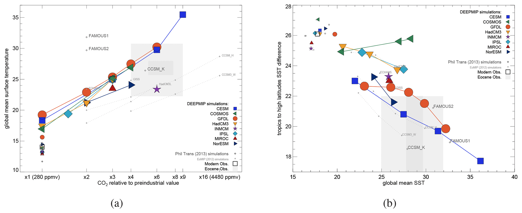
Figure 1(a) Global annual mean near-surface (2 m) air temperature in the DeepMIP simulations, as a function of atmospheric CO2. Large coloured symbols show the Eocene simulations, and smaller coloured symbols show the associated preindustrial controls. Also shown are results from some previous Eocene simulations (Lunt et al., 2012; Kiehl and Shields, 2013; Sagoo et al., 2013) and associated preindustrial control simulations (small grey symbols). The models that have carried out Eocene simulations at more than one CO2 concentration are joined by a straight line. The open square shows modern observations. The grey filled boxes show estimates of the global mean temperature (from Inglis et al., 2020) and CO2 (from Anagnostou et al., 2020) derived from proxies. For temperature, the light grey box shows the 10 % to 90 % confidence interval and the dark grey box shows the 33 % to 66 % confidence interval; for CO2, the light grey box shows ±1 SD and the dark grey box shows ±2 SD; see Sect. 3.4 for more details. Panel (b) is the same as panel (a) but for the meridional SST gradient as a function of global mean SST. The meridional SST gradient is defined here as the average SST equatorwards of ±30∘ minus the average SST polewards of ±60∘. The grey filled boxes show estimates of the global mean SST (from Inglis et al., 2020) and SST gradient (from Cramwinckel et al., 2018; Evans et al., 2018; Zhu et al., 2019) derived from proxies. For SST, the light grey box shows the 10 % to 90 % confidence interval and the dark grey box shows the 33 % to 66 % confidence interval; for the meridional temperature gradient, the light grey box shows the range (which extends below the y axis limit, down to 14 ∘C); see Sect. 3.4 for more details.
Figure 1a shows the global mean near-surface air temperature as a function of model CO2 for each DeepMIP simulation and associated preindustrial control as well as some previous Eocene simulations carried out with other boundary conditions (Lunt et al., 2012; Kiehl and Shields, 2013; Sagoo et al., 2013). The DeepMIP simulations are fairly consistent in terms of global mean temperature for a given CO2 concentration across the ensemble. The exception to this is INMCM, which at × 6 CO2 has a lower global mean temperature than any of the × 3 simulations. This is consistent with the fact that INMCM has the lowest climate sensitivity of all the models in the CMIP6 ensemble (Zelinka et al., 2020). With the exception of INMCM, the spread in the DeepMIP simulations is substantially less than in the previous Eocene simulations. In particular, at × 3 CO2, the CESM, COSMOS, GFDL, HadCM3, IPSL, and MIROC simulations are within 1.9 ∘C, compared with 5.0 ∘C at × 4 for the previous simulations. Part of the reason for the reduced spread of many of the DeepMIP simulations compared with previous simulations may be related to the fact that all of the DeepMIP model simulations have the same prescribed paleogeography, land–sea mask, and vegetation, whereas previous simulations used a variety of these boundary conditions.
The DeepMIP models have a range of Eocene climate sensitivities to CO2 doubling: from a minimum of 2.9 ∘C (for NorESM) to a maximum of 5.6 ∘C (for IPSL, excluding the anomalously warm × 9 CESM simulation). The average of the DeepMIP climate sensitivities (again excluding the × 9 CESM simulation) is 4.5 ∘C, which is greater than the average of the previous simulations (3.3 ∘C). There is a non-linearity (i.e. a global mean temperature that increases with CO2 differently than would be expected from a purely logarithmic relationship) in the CESM model simulations (as previously noted by Zhu et al., 2019) as well as in HadCM3 and (to a lesser extent) GFDL and COSMOS. In CESM, the climate sensitivity, normalized to a CO2 doubling, increases from 4.2 ∘C at × 1 to 4.8 and 9.7 ∘C at × 3 and × 6 respectively. In GFDL, the climate sensitivity increases from 3.7 ∘C at × 1 to 5.1 ∘C at × 3, but it then decreases to 4.7 ∘C at × 4. In HadCM3, the climate sensitivity increases from 3.8 ∘C at × 1 to 6.6 ∘C at × 2. In COSMOS, the climate sensitivity decreases from 5.2 ∘C at × 1 to 4.2 ∘C at × 3. In CESM, the non-linearity has been shown to arise from an increase in the strength of the positive short-wave cloud feedback as a function of temperature (Zhu et al., 2019); this is most apparent in the transition from × 6 to × 9.
CESM, COSMOS, GFDL, and HadCM3 all carried out simulations at × 1 CO2; comparison with the associated preindustrial controls indicates that the non-CO2 component of global warmth (i.e. due to changes in paleogeography, vegetation, and aerosols, and the removal of continental ice sheets) is 5.1, 3.6, 3.5, and 3.1 ∘C for CESM, GFDL, HadCM3, and COSMOS respectively. This is for comparison with previous simulations using CCSM3 (Caballero and Huber, 2013) that indicated a non-CO2 warming of ∼5∘C.
The latitudinal gradient of SST, defined here as the average SST equatorwards of ±30∘ minus the average temperature polewards of ±60∘, is shown in Fig. 1b. All DeepMIP models that have carried out simulations at more than one CO2 concentration show a decrease in the meridional SST gradient as temperature increases, apart from COSMOS. COSMOS also has the strongest preindustrial meridional temperature gradient. The × 1 CO2 Eocene simulations indicate that the non-CO2 DeepMIP boundary conditions decrease the latitudinal gradient by 3.4 ∘C for GFDL, 3.3 ∘C for CESM, 2.1∘ for COSMOS, and 0.8 ∘C for HadCM3. The GFDL model displays a markedly non-linear response, with a more rapidly decreasing temperature gradient as a function of temperature at higher temperatures than at lower temperatures. In contrast to the global mean temperature, the DeepMIP models show substantial spread in the meridional temperature gradient across the ensemble; COSMOS has a particularly strong gradient in the Eocene at × 3 and × 4 CO2, and HadCM3 and IPSL also have relatively strong gradients, similar to previous Eocene simulations with HadCM3L (Lunt et al., 2010b).
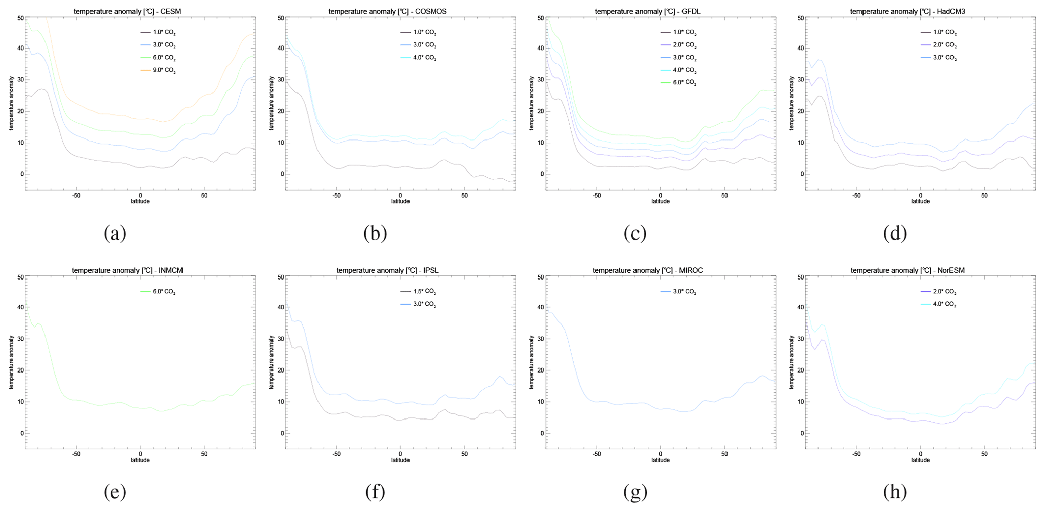
Figure 2Zonal mean near-surface air temperatures in the DeepMIP simulations, as a function of latitude and prescribed atmospheric CO2 concentration, expressed as anomalies relative to the equivalent preindustrial control for (a) CESM, (b) COSMOS, (c) GFDL, (d) HadCM3, (e) INMCM, (f) IPSL, (g) MIROC, and (h) NorESM.
The zonal mean near-surface air temperature anomaly, relative to the preindustrial simulation, as a function of latitude is shown in Fig. 2. Polar amplification is clear in both hemispheres for all models at CO2 1. There is greater amplification in the Southern Hemisphere than in the Northern Hemisphere, due to the replacement of the Antarctic ice sheets with vegetated land surface, with associated local warming due to the altitude and albedo change. There is a similar pattern of response across the models for a given CO2 concentration. However, although the models have a similar response in the Southern Hemisphere, the CESM model has greater polar amplification than other models in the Northern Hemisphere for a given CO2 concentration (in particular at × 3 CO2). The pattern of warming in the × 1 simulations is similar between the CESM, GFDL, and HadCM3 models. In particular, they all exhibit warming around 30–40∘ N, which coincides with lower topography in the Tibetan Plateau region in the Eocene relative to the preindustrial period. There is also consistent warming in the Northern Hemisphere Arctic (except for COSMOS) that coincides with the absence of the Greenland ice sheet and boreal forest in place of tundra and bare soil in the preindustrial period. The same underlying structure is seen in the higher CO2 simulations (see, for example, GFDL, Fig. 2b).
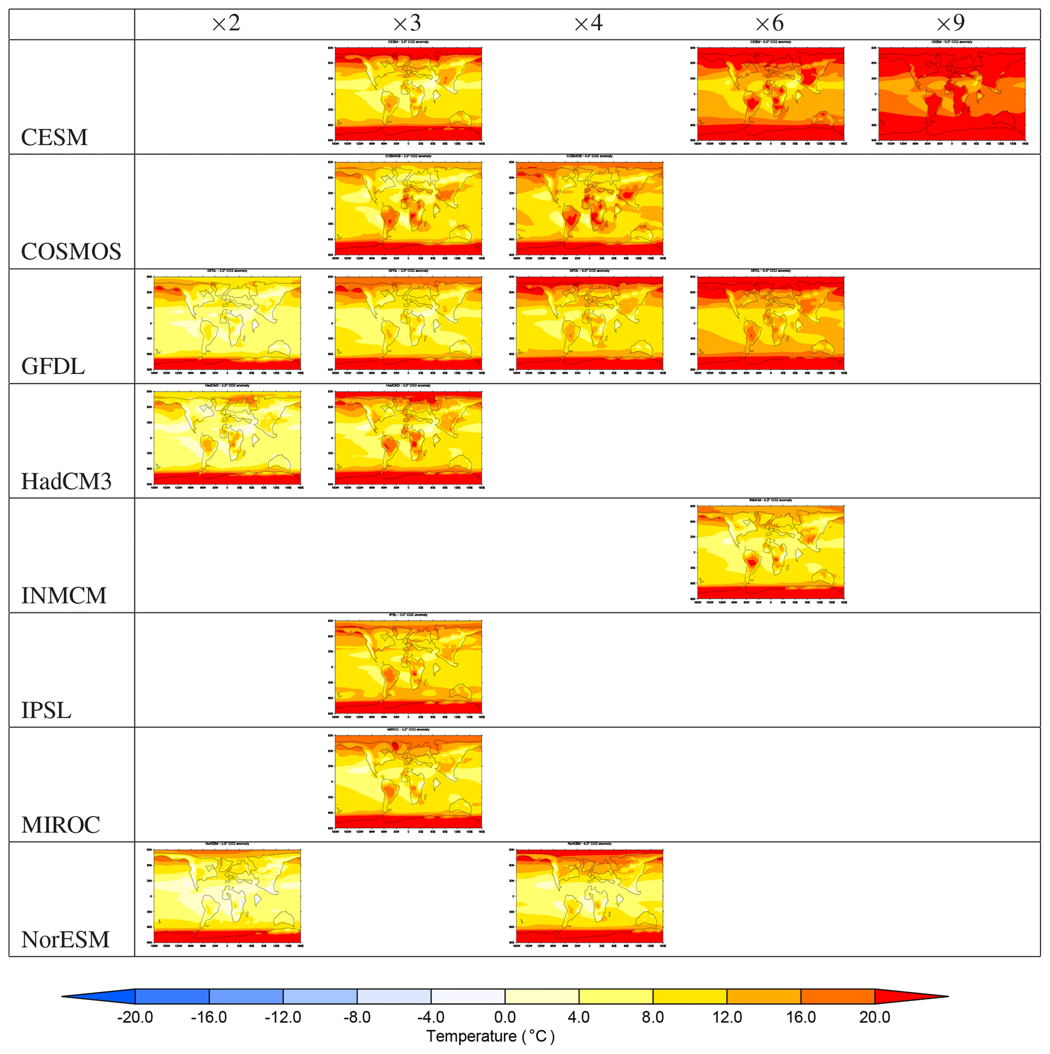
Figure 3DeepMIP near-surface air temperature anomalies, relative to the zonal mean of the associated preindustrial simulation, ordered by CO2 concentration and by model. Simulations with CO2 equal or greater than × 2 are shown. The variable plotted is in the notation of Lunt et al. (2012).
The spatial pattern of surface air temperature response is shown in Fig. 3. Because of the variation in continental positions between the preindustrial and Eocene periods, we show the difference between the Eocene and the zonal mean of the preindustrial simulation, i.e. in the notation of Lunt et al. (2012). This shows some consistent responses across the ensemble. In particular, in addition to the polar amplification, the response is characterized by greater warming over land than over ocean. Many of the continental regions where the warming is more muted (such as the Rockies, tropical east Africa, India, and the mid-latitudes of East Asia) are associated with regions of high topography in the Eocene. There is also substantial warming in the North Pacific in all simulations. This may be associated with deep-water formation in this region driving poleward heat transport in the Pacific, but the ocean circulation in these simulations will be explored in a subsequent study.
A similar plot, but without the zonal mean of the preindustrial simulation (i.e. ), is shown in Fig. S1. Figure S1 also includes the Eocene simulations at × 1 and × 1.5. The Eocene × 1 simulations minus the preindustrial simulations show the spatial impact of the changes to the non-CO2 boundary conditions. Consistent across the ensemble is the clear warming in Antarctica associated with the altitude and albedo change, warming in the Tibetan Plateau associated with altitude change, and cooling in Europe.
3.3 Reasons for model spread
Here, we first qualitatively explore the different model results by presenting the changes in albedo and emissivity across the ensemble. We then quantitatively relate these to the zonal mean temperature change and global metrics by making use of a 1D energy balance framework. Future work in the framework of DeepMIP will explore the model simulations in more detail, in particular the response of clouds, the hydrological cycle, and ocean circulation.
The patterns of surface albedo in the preindustrial and Eocene simulations are shown in Fig. S2. The lower albedo associated with the lack of Antarctic ice sheet in the Eocene is clear for all the models. In addition, the Eocene models do not have the high albedo associated with modern subtropical deserts (the Eocene experimental design specified average soil properties to be prescribed for all non-vegetated surfaces). The gradual decrease in high-latitude albedo with increasing surface temperature is apparent in all models, over both land and ocean, due to decreasing snow and sea ice cover. GFDL has a relatively low albedo prescribed over land in the preindustrial simulation, which is consistent with its relatively warm global mean (Fig. 1a; small red circle). CESM generally retains more snow cover than other models over Antarctica for a given CO2 concentration. NorESM has a relatively low prescribed albedo over land in the Eocene. The patterns of planetary albedo in the preindustrial and Eocene simulations are shown in Fig. S3. Again, the high albedo over high-latitude regions is clear, although the planetary albedo over Antarctica in the preindustrial simulation is lower then the surface albedo, indicating that the presence of clouds lowers the albedo in this region. Globally, there is a transition to lower values as temperature increases, and the regions associated with the lowest values (e.g. the subtropics in CESM) tend to expand in area, associated with decreases in cloud cover and opacity (Zhu et al., 2019). However, GFDL retains a high planetary albedo in the Arctic, even at × 6 CO2, despite a low surface albedo, indicating persistent cloud cover in this region. MIROC appears to have less spatial structure in planetary albedo than the other models. The patterns of emissivity in the preindustrial and Eocene simulations are shown in Fig. S4. The relatively low emissivity associated with the high-altitude Antarctic ice sheet in the preindustrial simulation is apparent. The emissivity generally decreases as temperature increases, which is likely associated with increasing water vapour and changes in clouds, and the patterns remain fairly consistent as temperature increases, with the lowest values over the warm pool in the western tropical Pacific.
In order to quantitatively relate these differences in radiative fluxes to the differences in temperature presented in Sect. 3.2, we make use of the energy balance framework described in Heinemann et al. (2009) and used previously to explore Eocene simulations by Lunt et al. (2012). In this framework, the zonal mean surface temperature (τ), planetary albedo (αp), emissivity (ϵ), incoming TOA solar radiation (S), and meridional heat flux (H) are related by
where σ is the Stefan–Boltzmann constant, and αp, ϵ, H, and S are functions of latitude that can be derived from the modelled energy fluxes, from either the preindustrial (xP1) or × N CO2 Eocene (xEN) simulations. In our case, the solar constant is the same in the preindustrial and Eocene simulations; thus, by rearranging Eq. (1), we can write τ as a function of αp, ϵ, and H. For example, the surface temperature of the standard Eocene × 3 simulation is and that of a preindustrial simulation is . The contribution of emissivity changes to the Eocene warming at × 3 relative to the preindustrial simulation, Δτϵ, is then given by , and similarly for meridional heat flux and planetary albedo:
Heinemann et al. (2009) and Lunt et al. (2012) showed how this framework could be expanded to also include terms related to long-wave and short-wave cloud changes by including terms derived from the clear-sky fluxes from the model radiation scheme. Here, we choose instead to partition the planetary albedo term () into a surface albedo term () and a non-surface albedo term () as follows:
where αs is the surface albedo. The surface albedo changes are a result of prescribed vegetation and ice sheet albedo changes as well as snow and sea ice feedbacks. The non-surface albedo changes are a result of cloud and aerosol changes or cloud masking effects (see below). Note that due to the non-linear dependence of albedo and emissivity on the radiative fluxes, the results are sensitive to the order of zonal mean, annual mean, and albedo and emissivity operators, but this has a generally small effect, except in the partitioning of surface and non-surface albedo in the high latitudes where it can have an effect of ±3 ∘C (not shown).
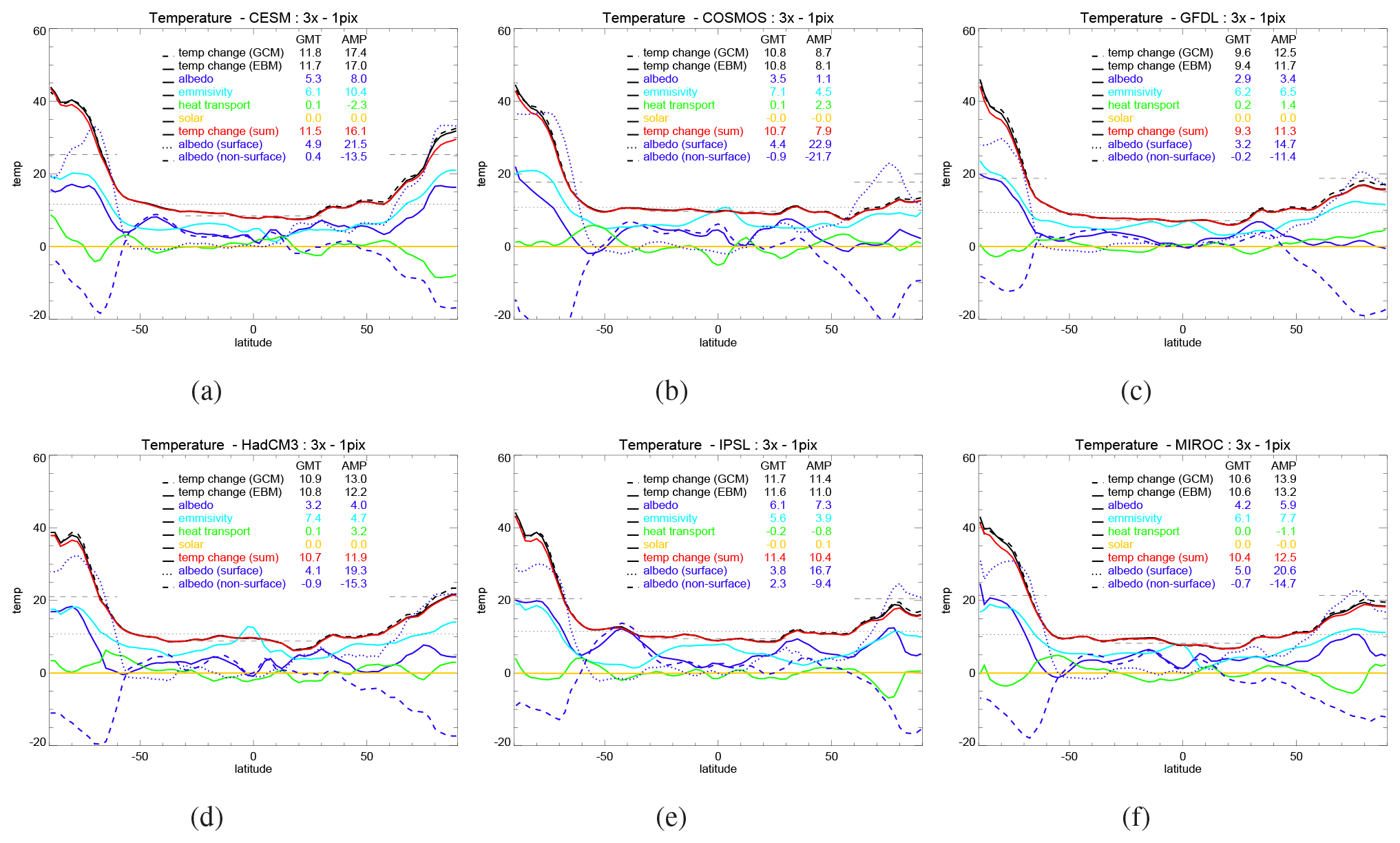
Figure 4The results of the energy balance analysis as described in Eqs. (2) and (3), applied to the differences between the DeepMIP × 3 simulations and their associated preindustrial controls. The black dashed line shows the zonal mean surface temperature changes directly from the general circulation models (GCMs). The black solid line shows the temperature change derived from the radiative fluxes, Δτ. Solid blue, cyan, and green lines show the contributions from planetary albedo (Δτϵ), emissivity (Δτϵ), and meridional heat flux (Δτϵ) respectively (Eq. 2). The blue dotted and dashed lines show the contribution from surface albedo () and non-surface albedo () respectively (Eq. 3). The red line shows the sum of the individual terms. For each model, the contribution of each term to the changes in global mean temperature (GMT) and the polar amplification (AMP; expressed as the difference in warming between the high latitudes, polewards of ±60∘, and the tropics, ±30∘) are quantified in the legend.
The results of this analysis are shown in Fig. 4 for the models that carried out × 3 simulations (all models except for INMCM and NorESM). This shows that all models generally have similar reasons for their response to the DeepMIP boundary conditions. In particular, in the equatorial region (latitudes ±10∘), the temperature response is generally dominated by emissivity changes; in the subtropics, it is dominated by emissivity and albedo (specifically, non-surface albedo) changes. In the Southern Hemisphere high latitudes, both emissivity and albedo changes contribute to warming. The change in altitude over Antarctica is likely a large part of this emissivity contribution. The albedo-induced change is made up of a large positive surface albedo contribution which is partially cancelled by a negative non-surface albedo contribution. This partial cancellation is a result of the very strong surface albedo change over Antarctica. In the absence of clouds, this surface albedo change on its own would cause large changes in temperature. However, in reality, some of these changes are masked by clouds and, as such, do not have as big an effect as would be the case in a cloud-free state. In the Northern Hemisphere, the signals are more variable across the ensemble. Most models show similar behaviour to the Southern Hemisphere, with positive contributions from emissivity and surface albedo and a negative contribution from non-surface albedo (again resulting from the cloud masking effect, over the Arctic sea ice). However, in COSMOS and GFDL, the Arctic response is dominated by emissivity changes, with relatively little contribution from albedo.
The global mean warming, × 3 minus preindustrial, is fairly constant across the ensemble. The greatest warming of 11.8 ∘C is observed in CESM, for which 6.1 ∘C comes from emissivity and 5.3 ∘C comes from albedo (4.9 ∘C from surface albedo and 0.4 ∘C from non-surface albedo). The lowest warming of 9.6 ∘C is observed in GFDL, for which 6.2 ∘C comes from emissivity and 2.9 ∘C comes from albedo (3.2 ∘C from surface albedo and −0.2 ∘C from non-surface albedo). Therefore, the difference in sensitivity between these two end-members of the ensemble primarily results from reduced surface albedo change in GFDL compared with CESM, and secondarily from negative non-surface albedo changes in GFDL compared with positive in CESM.
The reasons for the polar amplification are more variable between the models. For the model with the greatest polar amplification, CESM (17.4 ∘C), this is made up of 8.0 ∘C from albedo, 10.4 ∘C from emissivity, and −2.3 ∘C from meridional heat flux. For the model with the least polar amplification, COSMOS (8.7 ∘C), this is made up of 1.1 ∘C from albedo, 4.5 ∘C from emissivity, and 2.3 ∘C from meridional heat flux. Other models share relatively similar polar amplification (ranging from 11.4 ∘C in IPSL to 13.9 ∘C in MIROC), but the reasons for this vary between the models; in IPSL the dominant contribution is from albedo, in GFDL it is from emissivity with a positive contribution from meridional heat flux, in MIROC it is also from emissivity but with a negative contribution from meridional heat flux, and in HadCM3 it is roughly equal between albedo and emissivity, with a strong contribution from meridional heat flux.
The above-mentioned differences, × 3 minus preindustrial, can be considered as consisting of a component due to non-CO2 boundary condition changes (× 1 minus preindustrial) and a component due to CO2 change (× 3 minus × 1). Four of the models (CESM, COSMOS, GFDL, and HadCM3) also carried out simulations at × 1 which allow us to diagnose this partitioning. The energy balance analysis for × 1 minus preindustrial and × 3 minus × 1 is shown in Figs. S5 and S6 (note that due to non-linearities, the sum of these two partitions does not exactly equal the × 3 minus preindustrial values shown in Fig. 4). This shows that the non-CO2 response (Fig. S5) is greatest in the polar regions of the Southern Hemisphere, where albedo and emissivity contribute approximately equally in all models. Elsewhere, the signal is small; for the global mean, albedo and emissivity contribute roughly equally, although albedo dominates in CESM and emissivity dominates in GFDL. For the CO2-only response (Fig. S6), emissivity changes dominate in all models on a global scale. As expected, the contribution due to surface albedo changes is close to zero in all regions except the high latitudes. All models show polar amplification in both hemispheres, but the reasons for this vary. CESM polar amplification is due to both emissivity and albedo changes, and it is offset by changes in meridional heat flux, whereas the other models are dominated by emissivity and meridional heat flux changes and offset by albedo changes (due to strong offsetting by non-surface albedo). The importance of changes in outgoing long-wave radiation for polar amplification in response to CO2 forcing is also seen in model simulations of the modern climate (Pithan and Mauritsen, 2014).
Table 2Summary of the contributions to global mean surface warming and polar amplification from preindustrial to × 3. Values are shown for the four DeepMIP models that carried out simulations of the preindustrial, × 1, and × 3 (CESM, COSMOS, GFDL, and HadCM3). The values correspond to those shown in Figs. S5 and S6. Note that the sum of these is slightly different from the values in Fig. 4 due to non-linearities. Polar amplification is defined as the difference in warming between the high latitudes (polewards of ±60∘) and the tropics (±30∘).

By way of summary, the reasons for the ×3 minus preindustrial difference, for the four models for which we can carry out a full partitioning, are given in Table 2. This shows that, averaged across these four models, about 5 ∘C of the ∼ 10 ∘C warming arises from emissivity changes from the CO2 increase (and associated water vapour and long-wave cloud feedbacks); about 2 ∘C of the ∼ 10 ∘C warming arises from albedo changes from the non-CO2 boundary conditions, primarily removal of ice, and changes in vegetation and aerosols (and associated cloud, snow, and sea ice feedbacks); about 1.5 ∘C of the ∼ 10 ∘C warming arises from emissivity changes from the non-CO2 boundary conditions, primarily lower Antarctic altitude (and associated water vapour changes); and about 1.5 ∘C of the ∼ 10 ∘C warming arises from albedo changes from the CO2 increase (i.e. cloud, snow, and sea ice feedbacks). For polar amplification, about 5 ∘C of the ∼ 12 ∘C warming arises from the emissivity changes from the non-CO2 boundary conditions, about 4 ∘C of the ∼ 12 ∘C warming arises from the albedo changes from the non-CO2 boundary conditions, about 2 ∘C of the ∼ 12 ∘C warming arises from emissivity changes from the CO2 increase, and about 1 ∘C of the ∼ 12 ∘C warming arises from heat flux changes (made up of a contribution of +2 ∘C from the CO2 increase and −1 ∘C from the non-CO2 changes).
3.4 Model–data comparison
Here, we present a comparison of the models with proxy data of Eocene temperature and CO2. After introducing the proxy datasets, we compare the models to proxy-based global metrics and then to specific locations on a point-to-point basis.
3.4.1 Proxy datasets
For point-to-point model–data comparisons, we use the SST and surface air temperature (SAT) datasets for the EECO compiled by (Hollis et al., 2019). Following their recommendation, we exclude δ18O-derived SST estimates from recrystallized planktonic foraminifera because these estimates are generally significantly cooler than estimates derived from the δ18O value of well-preserved foraminifera, foraminiferal Mg ∕ Ca ratios, and clumped isotope values from larger benthic foraminifera, due to diagenetic effects.
In terms of global metrics, we make use of the global mean near-surface air temperature (GSAT) estimate for the EECO from Inglis et al. (2020), which is based on the Hollis et al. (2019) temperature dataset and also excludes SST estimates from recrystallized foraminifera. The vertical dimensions of the grey filled boxes in Fig. 1a show the 33 % to 66 % and the 10 % to 90 % confidence intervals of this GSAT estimate. For the global mean SST, we again use the GSAT estimate of Inglis et al. (2020) but convert this to global mean SST using a linear function derived from the mean land–sea temperature contrast in all the model simulations shown in Fig. 1:
This SST estimate forms the horizontal dimensions of the grey filled boxes in Fig. 1b.
We make use of SST gradient estimates from Cramwinckel et al. (2018), Evans et al. (2018), and Zhu et al. (2019). Cramwinckel et al. (2018) define a meridional temperature gradient metric as the difference between the tropical mean SST (derived from TEX86) and deep-ocean temperatures (derived from δ18O), assuming that deep-ocean temperatures are an approximation of high-latitude SSTs. In this way, they reconstruct a metric at 50 Ma of about 20–22 ∘C (their Fig. 3b). Evans et al. (2018) employ a similar approach but using tropical SSTs and deep-ocean temperatures from Mg ∕ Ca between 48 and 56 Ma; they find a reduction in their metric from the modern to early Eocene of 22 % to 42 %. Given a modern gradient from HadISST (our Fig. 1b) of about 26 ∘C, this gives an early Eocene estimate of 17.7 ∘C (20.3 to 15.1 ∘C). Using a similar approach to Evans et al. (2018), Zhu et al. (2019) find a reduction in their metric of about 20 % to 45 % (their Fig. 1b), giving an estimate of 21 to 14 ∘C for the early Eocene. Given the differences in methodologies for deriving these estimates, the relatively wide time window of the “early Eocene” for two of the studies, and the differences between the proxy metrics and our modelled metric (defined here as the average SST equatorwards of ±30∘ minus the average SST polewards of ±60∘), we take the outer ranges of the three studies as our overall proxy estimate, giving a range from 14 to 22 ∘C. This range in the meridional temperature gradient estimate forms the vertical edge of the grey filled boxes in Fig. 1b. However, the use of benthic temperatures to approximate high-latitude annual mean surface temperature may result in biases due to the seasonality of deep-water formation (Evans et al., 2018), and we note that a detailed assessment of the meridional temperature gradient implied by proxies, similar to that carried out for global mean temperature by Inglis et al. (2020), would be beneficial for future model–data comparisons.
For CO2, Anagnostou et al. (2020) give two estimates of EECO CO2 based on two different calibrations, resulting in 95 % confidence intervals from 1170 to 1830 ppmv and from 1540 to 2490 ppmv. The uppermost and lowermost bounds of these two estimates are close to the × 4 (1120 ppmv) and × 9 (2520 ppmv) simulations; as such, these form the horizontal edges of the light grey box in Fig. 1. A normal distribution in absolute CO2 would give a corresponding 68 % confidence interval from 1470 to 2170 ppmv, and this forms the horizontal edges of the light grey box in Fig. 1.
Overall, for the purposes of describing the model–data consistency, we use “consistent” to describe a model that sits within the light grey boxes of Fig. 1a and b, and we use “very consistent” to describe a model that sits within the dark grey boxes of Fig. 1a and b.
3.4.2 Comparison with global metrics
For the DeepMIP models, only those that carried out simulations at × 4 CO2, × 6 CO2, or × 9 CO2 are consistent with the CO2 proxies (i.e. CESM, COSMOS, GFDL, INMCM, and NorESM), and only those that carried out simulations at × 6 CO2 are very consistent with the CO2 proxies (i.e. CESM, GFDL, and INMCM). All of these simulations are also consistent with the GSAT proxies, but only COSMOS and GFDL at × 4 are very consistent with the GSAT proxies (inspection of Fig. 1 indicates that CESM would also be very consistent with the GSAT proxies if there was a simulation at × 4). No simulations are very consistent with both the CO2 and GSAT proxies. Only CESM at × 6, GFDL at × 4 and × 6, and NorESM at × 4 are consistent with the CO2, GSAT, and meridional temperature gradient proxies.
Of the pre-DeepMIP simulations in Fig. 1a and b, CCSM_H and CCSM_W at × 8 are also consistent with all the proxy constraints, and CCSM_K is additionally very consistent with GSAT. However, as discussed in Sect. 1, CCSM_K includes somewhat arbitrary modifications to cloud parameters that are designed to enable the model to better fit the Eocene observations; as such, in contrast to the DeepMIP simulations, CCSM_K cannot be considered entirely independent of the temperature data.
Some quantitative metrics for the simulations are presented in Table S2. In this case, the metrics are given for the set of simulations that were carried out at CO2 concentrations consistent with the proxies.
3.4.3 Comparison with specific locations
The limited range of CO2 concentrations explored by some models, coupled with the relatively large uncertainties in EECO CO2 from proxies, means that a model–data comparison of individual model simulations with the site-by-site proxy data can be misleading. Therefore, we only conduct a detailed model–data comparison for models that provide simulations carried out under more than one CO2 concentration. For these models (CESM, COSMOS, GFDL, HadCM3, IPSL, and NorESM), we apply a global mean scaling factor to the simulated SST and GSAT such that the modelled global means best fit the global mean proxy data. We then compare the spatial patterns in the scaled model outputs with the spatial patterns in the site-by-site proxies. We provide a quantitative metric for the model–data fit and compare this with some idealized temperature distributions to put these metrics in context.
We scale the models by assuming that the spatial pattern of temperature change scales linearly with global mean temperature change and by interpolating or extrapolating to a global mean equal to the estimate from Inglis et al. (2020), i.e. 27 ∘C for near-surface air temperature, or an equivalent global mean SST given by Eq. (4). This process gives a scaling factor, s, that can be used to create a spatial field of implied temperature, Ti, which is consistent with this proxy-based global mean temperature, 〈Tp〉:
where LT and HT are the spatial fields of the two model simulations that have global means closest to 〈Tp〉, and 〈.〉 denotes a global mean quantity. This also allows us to calculate an inferred CO2 concentration, :
where HCO2 and LCO2 are the CO2 concentrations that correspond to the two simulations in Eq. (5). For surface air temperature, this process is equivalent to interpolating or extrapolating the straight lines in Fig. 1a to identify the CO2 concentration that corresponds to 〈Tp〉.
For CESM and GFDL, the scaling is found by interpolation (s<1.0) because there are simulations that are warmer than 〈Tp〉. For those models where the scaling extrapolates beyond the model simulations (i.e. s>1.0; COSMOS, HadCM3, IPSL, and NorESM), care must be taken due to the assumption of linearity. For HadCM3, IPSL, and COSMOS, this assumption is probably well justified (s=1.51, 1.37, and 1.05 respectively for the surface air temperature scaling), but for NorESM this assumption is probably poorly justified (s=2.02).
For HadCM3, GFDL, IPSL, CESM, COSMOS, and NorESM, the inferred CO2 concentrations for the surface air temperature scaling are 1030, 1050, 1080, 1130, 1140, and 2270 ppmv respectively. For CESM, COSMOS, and NorESM, these are consistent with the CO2 proxy estimates of 1120–2520 ppmv (Sect. 3.4.1); the other models have a slightly lower inferred CO2 concentrations than the proxies indicate. All of these inferred CO2 values are below the concentration at which the respective models are known to crash (see Sect. 3.1). When the same method is applied to the Lunt et al. (2012) simulations, the inferred CO2 are all higher than the proxy estimates (2640 ppmv for HadCM3L, 3300 ppmv for CCSM3_H, and 6210 ppmv for CCSM_W). Figure 1 indicates that these relatively cool Lunt et al. (2012) simulations are related to a relatively low climate sensitivity for CCSM3_H and CCSM3_W and to a relatively low response to non-CO2 forcing for HadCM3L and CCSM3_W.
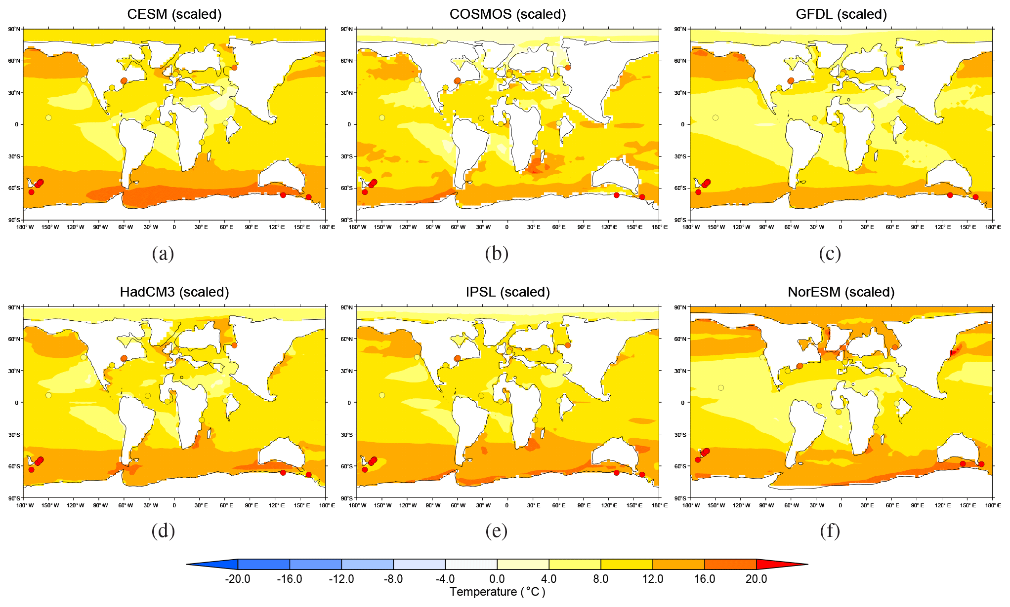
Figure 5Modelled SST anomalies for the Eocene, relative to the zonal mean of the associated preindustrial simulation. The variable plotted is in the notation of Lunt et al. (2012). The Eocene simulations have been scaled using a global tuning factor, as described in the text, so that they best fit the global mean SST data inferred from Inglis et al. (2020) (see Eqs. 5 and 4). As such, only models that carried out simulations with more then one CO2 concentration are shown: (a) CESM, (b) COSMOS, (c) GFDL, (d) HadCM3, (e) IPSL, and (f) NorESM. Also shown are the proxy SST estimates from Hollis et al. (2019) for the EECO, excluding those sites that they identified as being affected by diagenesis.
The scaled SST anomalies, relative to the zonal mean of the preindustrial modelled SST, for CESM, COSMOS, GFDL, HadCM3, IPSL, and NorESM, along with the proxy SST data from Hollis et al. (2019) (relative to the zonal mean of preindustrial observations), are shown in Fig. 5. In general, the models agree reasonably well with the tropical and mid-latitude SST data, but there is a large model–data inconsistency in the southwest Pacific sites around New Zealand and south of Australia, where the modelled anomalies are colder than proxy estimates by 5–10 ∘C. The reader is also referred to Fig. S7 for the modelled absolute SSTs and absolute SST proxy data.
The RMS skill score of the scaled absolute simulations, relative to the SST proxies, σs (∘C), is 7.0 for NorESM, 9.6 for GFDL, 9.7 for CESM, 10.5 for HadCM3, 10.7 for IPSL, and 12.0 for COSMOS. Note that the NorESM score is not directly comparable to the others because the NorESM simulation, and the proxy data it is compared with, are on a paleomagnetic reference frame rather than a mantle reference frame (Fig. 5f). For comparison, the GFDL skill score is 7.3 when calculated on the paleomagnetic reference frame. Note that we calculate all RMS scores from a specific point-to-point comparison of models and data, not from zonal means.
To put these numbers in context, we also calculate the same skill score for some idealized temperature distributions (on the mantle reference frame), expressed as anomalies relative to the zonal mean of the preindustrial observations. This approach is similar to that used by Hargreaves et al. (2013) in the context of Quaternary model–data comparisons. Our idealized temperature distributions are (i) a constant value of zero (i.e. no change from the zonal mean of the preindustrial simulation), (ii) a non-zero constant value (C), and (iii) a function . For the constant value, C, we choose a value that is equal to an estimate of global mean SST change from the proxies. This estimate of SST change is scaled from the proxy-based estimate of GSAT, 〈Tp〉=27 ∘C, using the scaling in Eq. (4), minus the preindustrial global mean SST. For the function f(ϕ), we choose A and B such that the global mean is equal to C, and the polar amplification metric, defined as the average SST equatorwards of ±30∘ minus the average SST polewards of ±60∘, is equal to our central estimate, i.e. 18 ∘C minus the preindustrial value (see Sect. 3.4.1).
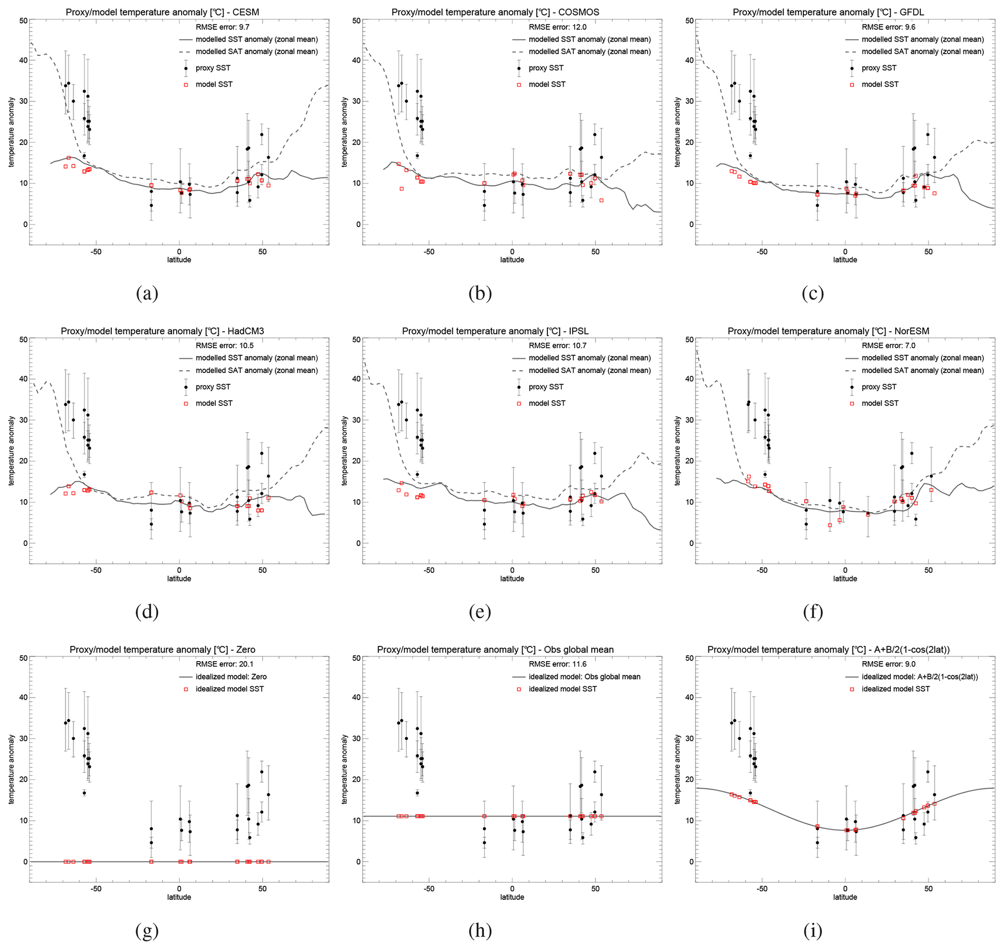
Figure 6(a–d) Zonal mean SST (solid lines) and near-surface air temperature (dashed line) anomalies, relative to the zonal mean of the associated preindustrial simulation, for the scaled version of the (a) CESM, (b) COSMOS, (c) GFDL, (d) HadCM3, (e) IPSL, and (f) NorESM models. Also shown are the EECO SSTs and error bars from Hollis et al. (2019), expressed as a difference relative to the zonal mean of the preindustrial observations. Panels (g)–(i) are the same as panels (a)–(f) but instead of a model we show idealized temperature distributions of (g) 0, (h) C, and (i) . All plots also show the proxy SST estimates from Hollis et al. (2019) for the EECO, excluding those sites that they identified as being affected by diagenesis (black circles with uncertainty bars). The modelled and idealized SSTs at the specific location of the proxies (red squares) are also displayed.
These idealized functions are shown in Fig. 6g–i as zonal means, along with the scaled DeepMIP models (Fig. 6a–f), and are all expressed as anomalies relative to the zonal mean of the preindustrial simulation. The global anomaly of zero relative to the zonal mean of the preindustrial simulation is associated with an RMS skill score σs=20.1, the global mean constant temperature anomaly (C) is associated with σs=11.6, and the f(ϕ) temperature profile is associated with σs=9.0 (σs=7.5 on the paleomagnetic reference frame). This means that all of the models apart from COSMOS can be considered as having some skill in capturing the first-order patterns of SST change (because the skill score of those models is better than that of the global constant), but only NorESM has skill in capturing the second-order, more regional temperature patterns (because the skill score of the other models is worse than that of the f(ϕ) distribution when calculated on the appropriate reference frame). However, the performance of the scaled NorESM simulations should be viewed with some caution because of its relatively high scaling factor (s, in Eq. 5).
So far, this analysis has focused on SSTs, but we also carry out a comparison with terrestrial near-surface air temperature data (SAT), even though it is generally less well constrained in age than SSTs and, as such, likely represents a wider range of climate states. The absolute SAT model–data comparison for each DeepMIP simulation is shown in Fig. S8. For those models that carried out more than one CO2 simulation (CESM, COSMOS, GFDL, HadCM3, IPSL, and NorESM), Figs. S9 and S10 show the SATs from the scaled models in comparison with terrestrial proxy data.
These figures show that both models and SAT terrestrial proxies show a similar amount of polar amplification. In particular, the southwest Pacific site SATs are better simulated in the models than the SSTs; the RMS skill score decreases in the southwest Pacific by 30 % on average for the SATs compared with the SSTs across the ensemble. This implies that there may be inconsistency between marine and terrestrial temperatures in either the proxies or models in this region. This discrepancy could be related to a potential summer bias in mid- and high-latitude SST proxies (Hollis et al., 2012; Davies et al., 2019). An alternative hypothesis is that the discrepancy is related to Red Sea-like features of GDGT (glycerol dialkyl glycerol tetraethers) distributions in high SST samples from the southwest Pacific and Wilkes Land that appear to amplify proxy SSTs where isoGDGTRS>30 (Inglis et al., 2015), which is an idea supported by recent work in the context of the Cretaceous (Steinig et al., 2020). However, the discrepancy may also be caused by physical processes that are not captured by any of the models.
We have presented an ensemble of model simulations of the Eocene, carried out in the framework of DeepMIP. The focus has been on documenting the annual mean modelled temperatures, exploring the reasons for the different responses in the models, and comparing with proxy data. Compared with previous model simulations, the results show reduced spread across the ensemble (except for the INMCM model) and greater climate sensitivity on average. The contribution to Eocene warmth from non-CO2 boundary conditions (paleogeography and vegetation and aerosols) is between 3.1 ∘C (HadCM3) and 5.1 ∘C (CESM). The reasons for the model spread is explored using an energy balance framework. This indicates that the difference between the models with the greatest and least warming in the Eocene at × 3 CO2 is primarily due to differences in the surface albedo response and that the difference between the models with the greatest and least polar amplification in the Eocene is primarily due to differences in the albedo and emissivity response. Across the model ensemble, the global mean warming in the Eocene compared with preindustrial simulations arises mostly from changes in emissivity due to the elevated CO2 and associated water vapour and long-wave cloud feedbacks, whereas, in terms of the meridional temperature gradient, the reduction in the Eocene is primarily due to emissivity and albedo changes due to the non-CO2 boundary conditions (i.e. the removal of the Antarctic ice sheet and changes in vegetation). Due to the limited range of prescribed CO2 in the model simulations, coupled with uncertainties in proxy reconstructed CO2, we interpolate and extrapolate between simulations at multiple CO2 concentrations to infer the concentration that gives the best fit to previous estimates of the global mean temperature; we then compare the model-inferred temperatures to the proxy SSTs on a point-to-point basis. This shows that CESM, GFDL, HadCM3, IPSL, and NorESM all have “skill” in representing the first-order patterns in the SST proxies in that they show better agreement with the proxies than a tuned global constant warming. However, they do not reproduce the exceptional warmth in the southwest Pacific proxy SSTs, although the modelled and proxy SATs are in better agreement than SSTs in this region, pointing to a possible inconsistency between the marine and terrestrial paleotemperatures in either the models or the proxies. Despite the regional limitations in the SST model–proxy consistency, the scaled CESM, COSMOS, and NorESM models all simulate a best fit global mean temperature at CO2 concentrations that are consistent with the CO2 proxies, without prescribing changes to model parameters such as those related to clouds. Furthermore, CESM, GFDL, and NorESM are all consistent with the global mean temperature, meridional temperature gradient, and CO2 proxies. Tighter constraints from proxies on both CO2 and temperature would allow for better discrimination of the DeepMIP models and model simulations. It is worth noting that CESM and GFDL both implemented modified aerosols in their Eocene simulations (see Sect. 2.2); the importance of this remains a topic for further investigation. Other future work in the framework of DeepMIP will explore the model simulations and model–data comparisons in more detail, in particular the response of clouds, the hydrological cycle, and ocean circulation.
The model results, in terms of annual mean near-surface air temperature, SST, and radiative fluxes, for the Eocene and preindustrial control simulations, are available in the Supplement as netCDF files. These are derived from files in version 1.0 of the DeepMIP model database by interpolating to a common grid (3.75∘ longitude ×2.5∘ latitude) using climate data operators (CDOs). Bilinear interpolation is used for the near-surface air temperature data, and nearest-neighbour interpolation is used for the SST data. Access to the full DeepMIP model database can be requested from the corresponding author. The proxy database used in this study is identical to that used in Inglis et al. (2020) and is available from the Supplement of that study. This contains the same data as in Hollis et al. (2019), i.e. version 0.1 of the DeepMIP proxy database.
The supplement related to this article is available online at: https://doi.org/10.5194/cp-17-203-2021-supplement.
All authors contributed to the writing of the paper. DJL carried out the analysis. The model simulations were carried out by JZ (CESM), IN (COSMOS), DKH (GFDL), FB and SS (HadCM3), PM and EMV (INMCM), JBL, PS and YD (IPSL), WLC (MIROC), and ZZ (NorESM) with support from CLP and JET (CESM), GK and GL (COSMOS), AMdB and HKC (GFDL), PJV (HadCM3), AAO (MIROC), and PML (NorESM). EA and GF provided the CO2 data, and CHL and GNI provided input on the model–data comparisons. CJH and TDJ led the compilation of the DeepMIP database. DJL, MH, and BLOB coordinated the study.
The authors declare that they have no conflict of interest.
This article is part of the special issue “Paleoclimate Modelling Intercomparison Project phase 4 (PMIP4) (CP/GMD inter-journal SI)”. It is not associated with a conference.
Daniel J. Lunt, Sebastian Steinig, Paul Valdes, and Fran Bragg acknowledge funding from the NERC SWEET grant (grant no. NE/P01903X/1). Daniel J. Lunt also acknowledges funding from NERC DeepMIP grant (grant no. NE/N006828/1) and the ERC (“The greenhouse earth system” grant; T-GRES, project reference no. 340923, awarded to Rich Pancost). Christopher J. Poulsen and Jessica E. Tierney acknowledge funding from the Heising-Simons Foundation (grant no. 2016-015). Jiang Zhu and Christopher J. Poulsen wish to thank Jeff Kiehl, Christine Shields, and Mathew Rothstein for providing the CESM code as well as boundary and initial condition files for the CESM simulations. Wing-Le Chan and Ayako Abe-Ouchi acknowledge funding from JSPS KAKENHI (grant no. 17H06104) and MEXT KAKENHI (grant no. 17H06323), and are grateful to JAMSTEC for use of the Earth Simulator. David K. Hutchinson and Agatha M. de Boer were supported by the Swedish Research Council (project no. 2016-03912) and FORMAS (project no. 2018-01621). Their numerical simulations were performed using resources provided by the Swedish National Infrastructure for Computing (SNIC) at NSC, Linköping. Pierre Sepulchre, Jean-Baptiste Ladant, and Yannick Donnadieu were granted access to the HPC resources of TGCC under the allocation no. 2019-A0050102212 made by GENCI. The HadCM3 simulations were carried out using the computational facilities of the Advanced Computing Research Centre, University of Bristol (http://www.bristol.ac.uk/acrc/, last access: 10 January 2021). Gordon N. Inglis acknowledges a Royal Society Dorothy Hodgkin Fellowship. Matthew Huber was funded by the US National Science Foundation (NSF; grant nos. ATM-0902780 and OCE-0902882). Bette L. Otto-Bliesner acknowledges the CESM project, which is primarily supported by the National Science Foundation (NSF). This material is based upon work supported by the National Center for Atmospheric Research (NCAR), which is a major facility sponsored by the NSF under cooperative agreement no. 1852977. Computing and data storage resources, including the Cheyenne supercomputer (https://doi.org/10.5065/D6RX99HX), were provided by the Computational and Information Systems Laboratory (CISL) at NCAR. Tom Dunkley Jones was supported by NERC (grant no. NE/P013112/1). Polina Morozova was supported by the state assignment project no. 0148-2019-0009.
This research has been supported by the NERC (grant no. NE/P01903X/1).
This paper was edited by Irina Rogozhina and reviewed by two anonymous referees.
Abelmann, A., Gersonde, R., Knorr, G., Zhang, X., Chapligin, B., Maier, E., Esper, O., Friedrichsen, H., Lohmann, G., Meyer, H., and Tiedemann, R.: The seasonal sea-ice zone in the glacial Southern Ocean as a carbon sink, Nat. Commun., 6, 8136, https://doi.org/10.1038/ncomms9136, 2015. a
Anagnostou, E., John, E. H., Babila, T. L., Sexton, P. F., Ridgwell, A., Lunt, D. J., Pearson, P. N., Chalk, T. B., Pancost, R. D., and Foster, G. L.: Proxy evidence for state-dependence of climate sensitivity in the Eocene greenhouse, Nat. Commun., 11, 4436, https://doi.org/10.1038/s41467-020-17887-x, 2020. a, b, c
Baatsen, M., van Hinsbergen, D. J. J., von der Heydt, A. S., Dijkstra, H. A., Sluijs, A., Abels, H. A., and Bijl, P. K.: Reconstructing geographical boundary conditions for palaeoclimate modelling during the Cenozoic, Clim. Past, 12, 1635–1644, https://doi.org/10.5194/cp-12-1635-2016, 2016. a
Barron, E. J.: Eocene equator-to-pole surface ocean temperatures: A significant climate problem?, Paleoceanography, 2, 729–739, https://doi.org/10.1029/PA002i006p00729, 1987. a
Beerling, D. and Royer, D.: Convergent Cenozoic CO2 history, Nat. Geosci., 4, 418–420, 2011. a
Bloch-Johnson, J., Pierrehumbert, R. T., and Abbot, D. S.: Feedback temperature dependence dtermines the risk of high warming, Geophys. Res. Lett., 42, 4973–4980, https://doi.org/10.1002/2015GL064240, 2015. a
Burke, K. D., Williams, J. W., Chandler, M. A., Haywood, A. M., Lunt, D. J., and Otto-Bliesner, B. L.: Pliocene and Eocene provide best analogs for near-future climates, P. Natl. Acad. Sci., 115, 13288–13293, https://doi.org/10.1073/pnas.1809600115, 2018. a, b
Caballero, R. and Huber, M.: State-dependent climate sensitivity in past warm climates and its implications for future climate projections, P. Natl. Acad. Sci., 110, 14162–14167, 2013. a
Carlson, H. and Caballero, R.: Atmospheric circulation and hydroclimate impacts of alternative warming scenarios for the Eocene, Clim. Past, 13, 1037–1048, https://doi.org/10.5194/cp-13-1037-2017, 2017. a
Carmichael, M. J., Lunt, D. J., Huber, M., Heinemann, M., Kiehl, J., LeGrande, A., Loptson, C. A., Roberts, C. D., Sagoo, N., Shields, C., Valdes, P. J., Winguth, A., Winguth, C., and Pancost, R. D.: A model–model and data–model comparison for the early Eocene hydrological cycle, Clim. Past, 12, 455–481, https://doi.org/10.5194/cp-12-455-2016, 2016. a
Chan, W.-L., Abe-Ouchi, A., and Ohgaito, R.: Simulating the mid-Pliocene climate with the MIROC general circulation model: experimental design and initial results, Geosci. Model Dev., 4, 1035–1049, https://doi.org/10.5194/gmd-4-1035-2011, 2011. a
Cramwinckel, M. J., Huber, M., Kocken, I. J., Agnini, C., Bijl, P. K., Bohaty, S. M., Frieling, J., Hilgen, A. G. F. J., Kip, E. L., Peterse, F., van der Ploegand, U., Röhl, R., Schouten, S., and Sluijs, A.: Synchronous tropical and polar temperature evolution in the Eocene, Nature, 559, 382–386, 2018. a, b, c, d
Davies, A., Hunter, S. J., Gréselle, B., Haywood, A. M., and Robson, C.: Evidence for seasonality in early Eocene high latitude sea-surface temperatures, Earth Planet. Sci. Lett., 519, 274–283, https://doi.org/10.1016/j.epsl.2019.05.025, 2019. a
de Lavergne, C., Falahat, S., Madec, G., Roquet, F., Nycander, J., and Vic, C.: Toward global maps of internal tide energy sinks, Ocean Model., 137, 52–75, https://doi.org/10.1016/j.ocemod.2019.03.010, 2019. a
Delworth, T. L., Broccoli, A. J., Rosati, A., Stouffer, R. J., Balaji, V., Beesley, J. A., Cooke, W. F., Dixon, K. W., Dunne, J., Dunne, K. A., Durachta, J. W., Findell, K. L., Ginoux, P., Gnanadesikan, A., Gordon, C. T., Griffies, S. M., Gudgel, R., Harrison, M. J., Held, I. M., Hemler, R. S., Horowitz, L. W., Klein, S. A., Knutson, T. R., Kushner, P. J., Langenhorst, A. R., Lee, H.-C., Lin, S.-J., Lu, J., Malyshev, S. L., Milly, P. C. D., Ramaswamy, V., Russell, J., Schwarzkopf, M. D., Shevliakova, E., Sirutis, J. J., Spelman, M. J., Stern, W. F., Winton, M., Wittenberg, A. T., Wyman, B., Zeng, F., and Zhang, R.: GFDL's CM2 Global Coupled Climate Models. Part I: Formulation and Simulation Characteristics, J. Climate, 19, 643–674, https://doi.org/10.1175/JCLI3629.1, 2006. a
Dufresne, J.-L., Foujols, M.-A., Denvil, S., Caubel, A., Marti, O., Aumont, O., Balkanski, Y., Bekki, S., Bellenger, H., Benshila, R., Bony, S., Bopp, L., Braconnot, P., Brockmann, P., Cadule, P., Cheruy, F., Codron, F., Cozic, A., Cugnet, D., de Noblet, N., Duvel, J.-P., Ethé, C., Fairhead, L., Fichefet, T., Flavoni, S., Friedlingstein, P., Grandpeix, J.-Y., Guez, L., Guilyardi, E., Hauglustaine, D., Hourdin, F., Idelkadi, A., Ghattas, J., Joussaume, S., Kageyama, M., Krinner, G., Labetoulle, S., Lahellec, A., Lefebvre, M.-P., Lefevre, F., Levy, C., Li, Z. X., Lloyd, J., Lott, F., Madec, G., Mancip, M., Marchand, M., Masson, S., Meurdesoif, Y., Mignot, J., Musat, I., Parouty, S., Polcher, J., Rio, C., Schulz, M., Swingedouw, D., Szopa, S., Talandier, C., Terray, P., Viovy, N., and Vuichard, N.: Climate Change Projections Using the IPSL-CM5 Earth System Model: From CMIP3 to CMIP5, Clim. Dynam., 40, 2123–2165, https://doi.org/10.1007/s00382-012-1636-1, 2013. a
Emile-Geay, J. and Madec, G.: Geothermal heating, diapycnal mixing and the abyssal circulation, Ocean Sci., 5, 203–217, https://doi.org/10.5194/os-5-203-2009, 2009. a
Evans, D., Sagoo, N., Renema, W., Cotton, L. J., Müller, W., Todd, J. A., Saraswati, P. K., Stassen, P., Ziegler, M., Pearson, P. N., Valdes, P. J., and Affek, H. P.: Eocene greenhouse climate revealed by coupled clumped isotope-Mg/Ca thermometry, P. Natl. Acad. Sci., 115, 1174–1179, https://doi.org/10.1073/pnas.1714744115, 2018. a, b, c, d, e
Farnsworth, A., Lunt, D. J., O'Brien, C. L., Foster, G. L., Inglis, G. N., Markwick, P., Pancost, R. D., and Robinson, S. A.: Climate Sensitivity on Geological Timescales Controlled by Nonlinear Feedbacks and Ocean Circulation, Geophys. Res. Lett., 46, 9880–9889, https://doi.org/10.1029/2019GL083574, 2019a. a
Farnsworth, A., Lunt, D. J., Robinson, S. A., Valdes, P. J., Roberts, W. H. G., Clift, P. D., Markwick, P., Su, T., Wrobel, N., Bragg, F., Kelland, S.-J., and Pancost, R. D.: Past East Asian monsoon evolution controlled by paleogeography, not CO2, Science Advances, 5, eaax1697, https://doi.org/10.1126/sciadv.aax1697, 2019b. a
Feng, R., Otto-Bliesner, B. L., Xu, Y., Brady, E., Fletcher, T., and Ballantyne, A.: Contributions of aerosol-cloud interactions to mid-Piacenzian seasonally sea ice-free Arctic Ocean, Geophys. Res. Lett., 46, 9920–9929, https://doi.org/10.1029/2019GL083960, 2019. a
Galbraith, E. D., Gnanadesikan, A., Dunne, J. P., and Hiscock, M. R.: Regional impacts of iron-light colimitation in a global biogeochemical model, Biogeosciences, 7, 1043–1064, https://doi.org/10.5194/bg-7-1043-2010, 2010. a
Gasson, E., Lunt, D. J., DeConto, R., Goldner, A., Heinemann, M., Huber, M., LeGrande, A. N., Pollard, D., Sagoo, N., Siddall, M., Winguth, A., and Valdes, P. J.: Uncertainties in the modelled CO2 threshold for Antarctic glaciation, Clim. Past, 10, 451–466, https://doi.org/10.5194/cp-10-451-2014, 2014. a
Gettelman, A., Kay, J. E., and Shell, K. M.: The Evolution of Climate Sensitivity and Climate Feedbacks in the Community Atmosphere Model, J. Climate, 25, 1453–1469, https://doi.org/10.1175/JCLI-D-11-00197.1, 2012. a
Gierz, P., Werner, M., and Lohmann, G.: Simulating climate and stable water isotopes during the Last Interglacial using a coupled climate‐isotope model, J. Adv. Model. Earth Sy., 9, 2027–2045, https://doi.org/10.1002/2017MS001056, 2017. a
Gong, X., Knorr, G., Lohmann, G., and Zhang, X.: Dependence of abrupt Atlantic meridional ocean circulation changes on climate background states, Geophys. Res. Lett., 40, 3698–3704, https://doi.org/10.1002/grl.50701, 2013. a
Green, J. A. M. and Huber, M.: Tidal dissipation in the early Eocene and implications for ocean mixing, Geophys. Res. Lett., 40, 2707–2713, https://doi.org/10.1002/grl.50510, 2013. a
Guo, C., Bentsen, M., Bethke, I., Ilicak, M., Tjiputra, J., Toniazzo, T., Schwinger, J., and Otterå, O. H.: Description and evaluation of NorESM1-F: a fast version of the Norwegian Earth System Model (NorESM), Geosci. Model Dev., 12, 343–362, https://doi.org/10.5194/gmd-12-343-2019, 2019. a
Hagemann, S. and Dümenil, L.: A parametrization of the lateral waterflow for the global scale, Clim. Dynam., 14, 17–31, https://doi.org/10.1007/s003820050205, 1998. a
Hargreaves, J. C., Annan, J. D., Ohgaito, R., Paul, A., and Abe-Ouchi, A.: Skill and reliability of climate model ensembles at the Last Glacial Maximum and mid-Holocene, Clim. Past, 9, 811–823, https://doi.org/10.5194/cp-9-811-2013, 2013. a
Hasumi, H.: CCSR Ocean Component Model (COCO) Version 2.1, Technical Report, The University of Tokyo, Tokyo, Japan, 2000. a
Haywood, A. M., Hill, D. J., Dolan, A. M., Otto-Bliesner, B. L., Bragg, F., Chan, W.-L., Chandler, M. A., Contoux, C., Dowsett, H. J., Jost, A., Kamae, Y., Lohmann, G., Lunt, D. J., Abe-Ouchi, A., Pickering, S. J., Ramstein, G., Rosenbloom, N. A., Salzmann, U., Sohl, L., Stepanek, C., Ueda, H., Yan, Q., and Zhang, Z.: Large-scale features of Pliocene climate: results from the Pliocene Model Intercomparison Project, Clim. Past, 9, 191–209, https://doi.org/10.5194/cp-9-191-2013, 2013. a
Heavens, N. G., Shields, C. A., and Mahowald, N. M.: A paleogeographic approach to aerosol prescription in simulations of deep time climate, J. Adv. Model. Earth Sy., 4, M11002, https://doi.org/10.1029/2012MS000166, 2012. a
Heinemann, M., Jungclaus, J. H., and Marotzke, J.: Warm Paleocene/Eocene climate as simulated in ECHAM5/MPI-OM, Clim. Past, 5, 785–802, https://doi.org/10.5194/cp-5-785-2009, 2009. a, b, c
Herold, N., Buzan, J., Seton, M., Goldner, A., Green, J. A. M., Müller, R. D., Markwick, P., and Huber, M.: A suite of early Eocene ( 55 Ma) climate model boundary conditions, Geosci. Model Dev., 7, 2077–2090, https://doi.org/10.5194/gmd-7-2077-2014, 2014. a, b, c, d, e, f, g, h, i, j, k
Hollis, C. J., Taylor, K. W. R., Handley, L., Pancost, R. D., Huber, M., Creech, J. B., Hines, B. R., Crouch, E. M., Morgans, H. E. G., Crampton, J. S., Gibbs, S., Pearson, P. N., and Zachos, J. C.: Early Paleogene temperature history of the Southwest Pacific Ocean: Reconciling proxies and models, Earth Planet. Sci. Lett., 349/350, 53–66, 2012. a
Hollis, C. J., Dunkley Jones, T., Anagnostou, E., Bijl, P. K., Cramwinckel, M. J., Cui, Y., Dickens, G. R., Edgar, K. M., Eley, Y., Evans, D., Foster, G. L., Frieling, J., Inglis, G. N., Kennedy, E. M., Kozdon, R., Lauretano, V., Lear, C. H., Littler, K., Lourens, L., Meckler, A. N., Naafs, B. D. A., Pälike, H., Pancost, R. D., Pearson, P. N., Röhl, U., Royer, D. L., Salzmann, U., Schubert, B. A., Seebeck, H., Sluijs, A., Speijer, R. P., Stassen, P., Tierney, J., Tripati, A., Wade, B., Westerhold, T., Witkowski, C., Zachos, J. C., Zhang, Y. G., Huber, M., and Lunt, D. J.: The DeepMIP contribution to PMIP4: methodologies for selection, compilation and analysis of latest Paleocene and early Eocene climate proxy data, incorporating version 0.1 of the DeepMIP database, Geosci. Model Dev., 12, 3149–3206, https://doi.org/10.5194/gmd-12-3149-2019, 2019. a, b, c, d, e, f, g, h, i
Huang, X., Stärz, M., Gohl, K., Knorr, G., and Lohmann, G.: Impact of Weddell Sea shelf progradation on Antarctic bottom water formation during the Miocene, Paleoceanography, 32, 304–317, https://doi.org/10.1002/2016PA002987, 2017. a
Huber, M. and Caballero, R.: The early Eocene equable climate problem revisited, Clim. Past, 7, 603–633, https://doi.org/10.5194/cp-7-603-2011, 2011. a, b, c
Hurrell, J. W., Holland, M. M., Gent, P. R., Ghan, S., Kay, J. E., Kushner, P. J., Lamarque, J. F., Large, W. G., Lawrence, D., Lindsay, K., Lipscomb, W. H., Long, M. C., Mahowald, N., Marsh, D. R., Neale, R. B., Rasch, P., Vavrus, S., Vertenstein, M., Bader, D., Collins, W. D., Hack, J. J., Kiehl, J. T., and Marshall, S.: The community earth system model: A framework for collaborative research, B. Am. Meteorol. Soc., 94, 1339–1360, https://doi.org/10.1175/BAMS-D-12-00121.1, 2013. a, b
Hutchinson, D. K., de Boer, A. M., Coxall, H. K., Caballero, R., Nilsson, J., and Baatsen, M.: Climate sensitivity and meridional overturning circulation in the late Eocene using GFDL CM2.1, Clim. Past, 14, 789–810, https://doi.org/10.5194/cp-14-789-2018, 2018. a, b, c
Hutchinson, D. K., Coxall, H. K., O'Regan, M., Nilsson, J., Caballero, R., and de Boer, A. M.: Arctic closure as a trigger for Atlantic overturning at the Eocene-Oligocene Transition, Nat. Commun., 10, 3797, https://doi.org/10.1038/s41467-019-11828-z, 2019. a
Inglis, G. N., Farnsworth, A., Lunt, D., Foster, G., Hollis, C., Pagani, M., Jardine, P., Pearson, P., Markwick, P., Raynman, L., Galsworthy, A., and Pancost, R.: Descent towards the Icehouse: Eocene sea surface cooling inferred from GDGT distributions, Paleoceanography, 30, 1000–1020, https://doi.org/10.1002/2014PA002723, 2015. a
Inglis, G. N., Bragg, F., Burls, N. J., Cramwinckel, M. J., Evans, D., Foster, G. L., Huber, M., Lunt, D. J., Siler, N., Steinig, S., Tierney, J. E., Wilkinson, R., Anagnostou, E., de Boer, A. M., Dunkley Jones, T., Edgar, K. M., Hollis, C. J., Hutchinson, D. K., and Pancost, R. D.: Global mean surface temperature and climate sensitivity of the early Eocene Climatic Optimum (EECO), Paleocene–Eocene Thermal Maximum (PETM), and latest Paleocene, Clim. Past, 16, 1953–1968, https://doi.org/10.5194/cp-16-1953-2020, 2020. a, b, c, d, e, f, g, h
Jungclaus, J. H., Keenlyside, N., Botzet, M., Haak, H., Luo, J.-J., Latif, M., Marotzke, J., Mikolajewicz, U., and Roeckner, E.: Ocean circulation and tropical variability in the coupled model ECHAM5/MPI-OM, J. Climate, 19, 3952–3972, https://doi.org/10.1175/JCLI3827.1, 2006. a
K-1 model developers: K-1 coupled model (MIROC) description, Technical Report, Center for Climate System Research (University of Tokyo), National Institute for Environmental Studies, Frontier Research Center for Global Change, Tokyo, Japan, 2004. a
Kageyama, M., Braconnot, P., Bopp, L., Caubel, A., Foujols, M.-A., Guilyardi, E., Khodri, M., Lloyd, J., Lombard, F., Mariotti, V., Marti, O., Roy, T., and Woillez, M.-N.: Mid-Holocene and Last Glacial Maximum climate simulations with the IPSL model – part I: comparing IPSL_CM5A to IPSL_CM4, Clim. Dynam., 40, 2447–2468, https://doi.org/10.1007/s00382-012-1488-8, 2013. a
Kay, J. E., Hillman, B. R., Klein, S. A., Zhang, Y., Medeiros, B., Pincus, R., Gettelman, A., Eaton, B., Boyle, J., Marchand, R., and Ackerman, T. P.: Exposing Global Cloud Biases in the Community Atmosphere Model (CAM) Using Satellite Observations and Their Corresponding Instrument Simulators, J. Climate, 25, 5190–5207, https://doi.org/10.1175/JCLI-D-11-00469.1, 2012. a
Kiehl, J. T. and Shields, C. A.: Sensitivity of the PalaeoceneEocene Thermal Maximum climate to cloud properties, Phil. Trans. R. Soc. A, 371, 20130093, https://doi.org/10.1098/rsta.2013.0093, 2013. a, b, c, d, e, f
Knorr, G. and Lohmann, G.: Climate warming during Antarctic ice sheet expansion at the Middle Miocene transition, Nat. Geosci., 7, 376–381, https://doi.org/10.1038/NGEO2119, 2014. a
Knorr, G., Butzin, M., Micheels, A., and Lohmann, G.: A warm Miocene climate at low atmospheric CO2 levels, Geophys. Res. Lett., 38, L20701, https://doi.org/10.1029/2011GL048873, 2011. a
Koch-Larrouy, A., Madec, G., Bouruet-Aubertot, P., Gerkema, T., Bessières, L., and Molcard, R.: On the transformation of Pacific Water into Indonesian Throughflow Water by internal tidal mixing, Geophys. Res. Lett., 34, L04604, https://doi.org/10.1029/2006GL028405, 2007. a, b
Lohmann, G., Pfeiffer, M., Laepple, T., Leduc, G., and Kim, J.-H.: A model–data comparison of the Holocene global sea surface temperature evolution, Clim. Past, 9, 1807–1839, https://doi.org/10.5194/cp-9-1807-2013, 2013. a
Lott, F.: Alleviation of Stationary Biases in a GCM through a Mountain Drag Parameterization Scheme and a Simple Representation of Mountain Lift Forces, Mon. Weather Rev., 127, 788–801, https://doi.org/10.1175/1520-0493(1999)127<0788:AOSBIA>2.0.CO;2, 1999. a
Lott, F. and Miller, M. J.: A new subgrid-scale orographic drag parametrization: Its formulation and testing, Q. J. Roy. Meteorol. Soc., 123, 101–127, https://doi.org/10.1002/qj.49712353704, 1997. a
Lunt, D. J., Foster, G. L., Haywood, A. M., and Stone, E. J.: Late Pliocene Greenland glaciation controlled by a decline in atmospheric CO2 levels, Nature, 454, 1102–1105, 2008. a
Lunt, D. J., Haywood, A. M., Schmidt, G. A., Salzmann, U., Valdes, P. J., and Dowsett, H. J.: Earth system sensitivity inferred from Pliocene modelling and data, Nat. Geosci., 3, 60–64, 2010a. a
Lunt, D. J., Valdes, P. J., Dunkley Jones, T., Ridgwell, A., Haywood, A. M., Schmidt, D. N., Marsh, R., and Maslin, M.: CO2-driven ocean circulation changes as an amplifier of Paleocene-Eocene thermal maximum hydrate destabilization, Geology, 38, 875–878, 2010b. a, b
Lunt, D. J., Dunkley Jones, T., Heinemann, M., Huber, M., LeGrande, A., Winguth, A., Loptson, C., Marotzke, J., Roberts, C. D., Tindall, J., Valdes, P., and Winguth, C.: A model–data comparison for a multi-model ensemble of early Eocene atmosphere–ocean simulations: EoMIP, Clim. Past, 8, 1717–1736, https://doi.org/10.5194/cp-8-1717-2012, 2012. a, b, c, d, e, f, g, h, i, j, k, l
Lunt, D. J., Farnsworth, A., Loptson, C., Foster, G. L., Markwick, P., O'Brien, C. L., Pancost, R. D., Robinson, S. A., and Wrobel, N.: Palaeogeographic controls on climate and proxy interpretation, Clim. Past, 12, 1181–1198, https://doi.org/10.5194/cp-12-1181-2016, 2016. a
Lunt, D. J., Huber, M., Anagnostou, E., Baatsen, M. L. J., Caballero, R., DeConto, R., Dijkstra, H. A., Donnadieu, Y., Evans, D., Feng, R., Foster, G. L., Gasson, E., von der Heydt, A. S., Hollis, C. J., Inglis, G. N., Jones, S. M., Kiehl, J., Kirtland Turner, S., Korty, R. L., Kozdon, R., Krishnan, S., Ladant, J.-B., Langebroek, P., Lear, C. H., LeGrande, A. N., Littler, K., Markwick, P., Otto-Bliesner, B., Pearson, P., Poulsen, C. J., Salzmann, U., Shields, C., Snell, K., Stärz, M., Super, J., Tabor, C., Tierney, J. E., Tourte, G. J. L., Tripati, A., Upchurch, G. R., Wade, B. S., Wing, S. L., Winguth, A. M. E., Wright, N. M., Zachos, J. C., and Zeebe, R. E.: The DeepMIP contribution to PMIP4: experimental design for model simulations of the EECO, PETM, and pre-PETM (version 1.0), Geosci. Model Dev., 10, 889–901, https://doi.org/10.5194/gmd-10-889-2017, 2017. a, b, c, d, e, f, g, h, i, j, k, l, m
Marsland, S. J., Haak, H., Jungclaus, J. H., Latif, M., and Rőske, F.: The Max-Planck-Institute global ocean/sea ice model with orthogonal curvilinear coordinates, Ocean Model., 5, 91–127, https://doi.org/10.1016/S1463-5003(02)00015-X, 2003. a
Masson-Delmotte, V., Schulz, M., Abe-Ouchi, A., Beer, J., Ganopolski, A., Rouco, J. G., Jansen, E., Lambeck, K., Luterbacher, J., Naish, T., Osborn, T., Otto-Bliesner, B., Quinn, T., Ramesh, R., Rojas, M., Shao, X., and Timmermann, A.: Information from Paleoclimate Archives, in: Climate Change 2013: The Physical Science Basis. Contribution of Working Group I to the Fifth Assessment Report of the Intergovernmental Panel on Climate Change, edited by: Stocker, T., Qin, D., Plattner, G.-K., Tignor, M., Allen, S., Boschung, J., Nauels, A., Xia, Y., Bex, V., and Midgley, P., Cambridge University Press, Cambridge, UK, 2013. a
Meraner, K., Mauritsen, T., and Voigt, A.: Robust increase in equilibrium climate sensitivity under global warming, Geophys. Res. Lett., 40, 5944–5948, https://doi.org/10.1002/2013GL058118, 2013. a
Müller, R. D., Sdrolias, M., Gaina, C., and Roest, W. R.: Age, spreading rates, and spreading asymmetry of the world's ocean crust, Geochem. Geophys. Geosyst., 9, Q04006, https://doi.org/10.1029/2007GC001743, 2008. a
Niezgodzki, I., Knorr, G., Lohmann, G., Tyszka, J., and Markwick, P. J.: Late Cretaceous climate simulations with different CO2 levels and subarctic gateway configurations: A model-data comparison, Paleoceanography, 32, 980–998, https://doi.org/10.1002/2016PA003055, 2017. a
Niezgodzki, I., Tyszka, J., Knorr, G., and Lohmann, G.: Was the Arctic Ocean ice free during the latest Cretaceous? The role of CO2 and gateway configurations, Global Planet. Change, 177, 201–212, https://doi.org/10.1016/j.gloplacha.2019.03.011, 2019. a
Otto-Bliesner, B. L., Brady, E. C., Fasullo, J., Jahn, A., Landrum, L., Stevenson, S., Rosenbloom, N., Mai, A., and Strand, G.: Climate Variability and Change since 850 CE: An Ensemble Approach with the Community Earth System Model, B. Am. Meteorol. Soc., 97, 735–754, https://doi.org/10.1175/BAMS-D-14-00233.1, 2015. a
Pfeiffer, M. and Lohmann, G.: Greenland Ice Sheet influence on Last Interglacial climate: global sensitivity studies performed with an atmosphere–ocean general circulation model, Clim. Past, 12, 1313–1338, https://doi.org/10.5194/cp-12-1313-2016, 2016. a
Pithan, F. and Mauritsen, T.: Arctic amplification dominated by temperature feedbacks in contemporary climate models, Nat. Geosci., 7, 181–184, 2014. a
Roberts, C. D., LeGrande, A. N., and Tripati, A. K.: Climate sensitivity to Arctic seaway restriction during the early Paleogene, Earth Planet. Sci. Lett., 286, 576–585, 2009. a
Roeckner, E., Bäuml, G., Bonaventura, L., Brokopf, R., Esch, M., Giorgetta, M., Hagemann, S., Kirchner, I., Kornbleuh, L., Manzini, E., Rhodin, A., Schlese, U., Schulzweida, U., and Tompkins, A.: The atmospheric general circulation model ECHAM 5. PART I: Model description, Report 349, Max-Planck Institut für Meteorologie, Hamburg, Germany, 140 pp., 2003. a
Sagoo, N., Valdes, P., Flecker, R., and Gregoire, L.: The Early Eocene equable climate problem: can perturbations of climate model parameters identify possible solutions?, Phil. Trans. R. Soc. A, 371, 20130123, https://doi.org/10.1098/rsta.2013.0123, 2013. a, b, c, d
Sepulchre, P., Caubel, A., Ladant, J.-B., Bopp, L., Boucher, O., Braconnot, P., Brockmann, P., Cozic, A., Donnadieu, Y., Dufresne, J.-L., Estella-Perez, V., Ethé, C., Fluteau, F., Foujols, M.-A., Gastineau, G., Ghattas, J., Hauglustaine, D., Hourdin, F., Kageyama, M., Khodri, M., Marti, O., Meurdesoif, Y., Mignot, J., Sarr, A.-C., Servonnat, J., Swingedouw, D., Szopa, S., and Tardif, D.: IPSL-CM5A2 – an Earth system model designed for multi-millennial climate simulations, Geosci. Model Dev., 13, 3011–3053, https://doi.org/10.5194/gmd-13-3011-2020, 2020. a, b, c
Simmons, H. L., Jayne, S. R., Laurent, L. C., and Weaver, A. J.: Tidally driven mixing in a numerical model of the ocean general circulation, Ocean Model., 6, 245–263, https://doi.org/10.1016/S1463-5003(03)00011-8, 2004. a
Sloan, L. and Barron, E. J.: A comparison of Eocene climate model results to quantified paleoclimatic interpretations, Palaeogeogr., Palaeocl., 93, 183–202, https://doi.org/10.1016/0031-0182(92)90096-N, 1992. a
Smagorinsky, J.: General Circulation Experiments with the Primitive Equations: I The Basic Experiment, Mon. Weather Rev., 91, 99–164, https://doi.org/10.1175/1520-0493(1963)091<0099:GCEWTP>2.3.CO;2, 1963. a
Smith, R., Jones, P., Briegleb, B., Bryan, F., Danabasoglu, G., Dennis, J., Dukowicz, J., Eden, C., Fox-Kemper, B., Gent, P., and Others: The parallel ocean program (POP) reference manual ocean component of the community climate system model (CCSM) and community earth system model (CESM), Report, LAUR-01853, National Center for Atmospheric Research, Boulder, CO, USA, 140 pp., 2010. a
Stärz, M., Jokat, W., Knorr, G., and Lohmann, G.: Threshold in North Atlantic-Arctic Ocean circulation controlled by the subsidence of the Greenland-Scotland Ridge, Nat. Commun., 8, 15681, https://doi.org/10.1038/ncomms15681, 2017. a
Stein, C. A. and Stein, S.: A model for the global variation in oceanic depth and heat flow with lithospheric age, Nature, 359, 123–129, https://doi.org/10.1038/359123a0, 1992. a, b
Steinig, S., Dummann, W., Park, W., Latif, M., Kusch, S., Hofmann, P., and Flögel, S.: Evidence for a regional warm bias in the Early Cretaceous TEX86 record, Earth Planet. Sci. Lett., 539, 116184, https://doi.org/10.1016/j.epsl.2020.116184, 2020. a
Stepanek, C. and Lohmann, G.: Modelling mid-Pliocene climate with COSMOS, Geosci. Model Dev., 5, 1221–1243, https://doi.org/10.5194/gmd-5-1221-2012, 2012. a
Stevens, B., Giorgetta, M., Esch, M., Mauritsen, T., Crueger, T., Rast, S., Salzmann, M., Schmidt, H., Bader, J., Block, K., Borkopf, R., Fast, I., Kinne, S., Kornblueh, L., Lohmann, U., Pincus, R., Reichler, T., and Roeckner, E.: Atmospheric component of the MPI‐M Earth System Model: ECHAM6, J. Adv. Model. Earth Sy., 5, 146–172, https://doi.org/10.1002/jame.20015, 2013. a
Takata, K., Watanabe, T., and Emori, S.: Development of the minimal advanced treatments of surface interaction and runoff, Global Planet. Change, 38, 209–222, 2003. a
Thibodeau, B., Not, C., Zhu, J., Schmittner, A., Noone, D., Tabor, C., Zhang, J., and Liu, Z.: Last Century Warming Over the Canadian Atlantic Shelves Linked to Weak Atlantic Meridional Overturning Circulation, Geophys. Res. Lett., 45, 12376–12385, https://doi.org/10.1029/2018GL080083, 2018. a
Tiedtke, M.: Representation of Clouds in Large-Scale Models, Mon. Weather Rev., 121, 3040–3061, https://doi.org/10.1175/1520-0493(1993)121<3040:ROCILS>2.0.CO;2, 1993. a
Vahlenkamp, M., Niezgodzki, I., De Vleeschouwer, D., Lohmann, G., Bickert, T., and Pälike, H.: Ocean and climate response to North Atlantic seaway changes at the onset of long-term Eocene cooling, Earth Planet. Sci. Lett., 498, 185–195, https://doi.org/10.1016/j.epsl.2018.06.031, 2018. a
Valdes, P. J., Armstrong, E., Badger, M. P. S., Bradshaw, C. D., Bragg, F., Crucifix, M., Davies-Barnard, T., Day, J. J., Farnsworth, A., Gordon, C., Hopcroft, P. O., Kennedy, A. T., Lord, N. S., Lunt, D. J., Marzocchi, A., Parry, L. M., Pope, V., Roberts, W. H. G., Stone, E. J., Tourte, G. J. L., and Williams, J. H. T.: The BRIDGE HadCM3 family of climate models: HadCM3@Bristol v1.0, Geosci. Model Dev., 10, 3715–3743, https://doi.org/10.5194/gmd-10-3715-2017, 2017. a, b, c, d
Volodin, E. M. and Kostrykin, S. V.: Aerosol block in climate model of INM RAS, Russ. Meteorol. Hydrol., 8, 5–17, 2016. a
Volodin, E. M. and Lykossov, V. N.: Parameterization of Heat and Moisture Transfer in the Soil-Vegetation System for Use in Atmospheric General Circulation Models: 2. Numerical Experiments in Climate Modeling, Izv. Atmos. Oceanic Phy., 34, 559–569, 1998. a
Volodin, E. M., Mortikov, E. V., Kostrykin, S. V., Galin, V. Y., Lykossov, V. N., Gritsun, A. S., Diansky, N. A., Gusev, A. V., and Iakovlev, N. G.: Simulation of the present-day climate with the climate model INMCM5, Clim. Dynam., 49, 3715–3734, 2017. a
Volodin, E. M., Mortikov, E. V., Kostrykin, S. V., Galin, V. Y., Lykossov, V. N., Gritsun, A. S., Diansky, N. A., Gusev, A. V., Iakovlev, N. G., Shestakova, A. A., and Emelina, S. V.: Simulation of the modern climate using the INM-CM48 climate model, Russ. J. Numer. Anal. M., 33, 367–374, https://doi.org/10.1515/rnam-2018-0032, 2018. a
Walliser, E. O., Lohmann, G., Niezgodzki, I., Tűtken, T., and Schőne, B. R.: Response of Central European SST to atmospheric pCO2 forcing during the Oligocene – A combined proxy data and numerical climate model approach, Palaeogeogr., Palaeocl., 459, 552–569, https://doi.org/10.1016/j.palaeo.2016.07.033, 2016. a
Walliser, E. O., Lohmann, G., Niezgodzki, I., and Schőne, B. R.: Inter-annual climate variability in Europe during the Oligocene icehouse, Palaeogeogr., Palaeocl., 475, 140–153, https://doi.org/10.1016/j.palaeo.2017.03.020, 2017. a
Wei, W. and Lohmann, G.: Simulated Atlantic multidecadal oscillation during the Holocene, J. Climate, 25, 6989–7002, https://doi.org/10.1175/JCLI-D-11-00667.1, 2012. a
Wei, W., Lohmann, G., and Dima, M.: Distinct modes of internal variability in the global meridional overturning circulation associated with the Southern Hemisphere westerly winds, J. Phys. Oceanogr., 42, 785–801, https://doi.org/10.1175/JPO-D-11-038.1, 2012. a
Winguth, A., Shellito, C., Shields, C., and Winguth, C.: Climate Response at the Paleocene-Eocene Thermal Maximum to Greenhouse Gas Forcing – A Model Study with CCSM3, J. Climate, 23, 2562–2584, 2010. a, b
Zelinka, M. D., Myers, T. A., McCoy, D. T., Po-Chedley, S., Caldwell, P. M., Ceppi, P., Klein, S. A., and Taylor, K. E.: Causes of Higher Climate Sensitivity in CMIP6 Models, Geophys. Res. Lett., 47, e2019GL085782, https://doi.org/10.1029/2019GL085782, 2020. a
Zhang, X., Lohmann, G., Knorr, G., and Xu, X.: Different ocean states and transient characteristics in Last Glacial Maximum simulations and implications for deglaciation, Clim. Past, 9, 2319–2333, https://doi.org/10.5194/cp-9-2319-2013, 2013. a
Zhang, X., Lohmann, G., Knorr, G., and Purcell, C.: Abrupt glacial climate shifts controlled by ice sheet changes, Nature, 512, 290–294, https://doi.org/10.1038/nature13592, 2014. a
Zhang, X., Knorr, G., Lohmann, G., and Barker, S.: Abrupt North Atlantic circulation changes in response to gradual CO2 forcing in a glacial climate state, Nat. Geosci., 10, 518–523, https://doi.org/10.1038/ngeo2974, 2017. a
Zhang, Y., Huck, T., Lique, C., Donnadieu, Y., Ladant, J.-B., Rabineau, M., and Aslanian, D.: Early Eocene vigorous ocean overturning and its contribution to a warm Southern Ocean, Clim. Past, 16, 1263–1283, https://doi.org/10.5194/cp-16-1263-2020, 2020. a, b
Zhang, Z. S., Nisancioglu, K., Bentsen, M., Tjiputra, J., Bethke, I., Yan, Q., Risebrobakken, B., Andersson, C., and Jansen, E.: Pre-industrial and mid-Pliocene simulations with NorESM-L, Geosci. Model Dev., 5, 523–533, https://doi.org/10.5194/gmd-5-523-2012, 2012. a
Zhu, J., Liu, Z., Brady, E., Otto-Bliesner, B., Zhang, J., Noone, D., Tomas, R., Nusbaumer, J., Wong, T., Jahn, A., and Tabor, C.: Reduced ENSO variability at the LGM revealed by an isotope-enabled Earth system model, Geophys. Res. Lett., 44, 6984–6992, https://doi.org/10.1002/2017GL073406, 2017a. a
Zhu, J., Liu, Z., Brady, E. C., Otto-Bliesner, B. L., Marcott, S. A., Zhang, J., Wang, X., Nusbaumer, J., Wong, T. E., Jahn, A., and Noone, D.: Investigating the direct meltwater effect in terrestrial oxygen-isotope paleoclimate records using an isotope-enabled Earth system model, Geophys. Res. Lett., 44, 12501–12510, https://doi.org/10.1002/2017GL076253, 2017b. a
Zhu, J., Poulsen, C. J., and Tierney, J. E.: Simulation of Eocene extreme warmth and high climate sensitivity through cloud feedbacks, Science Advances, 5, eaax1874, https://doi.org/10.1126/sciadv.aax1874, 2019. a, b, c, d, e, f, g, h