2.1 The model

We use the ECCO LLC270 physical fields (Zhang et al., 2018) to simulate the transport of alkalinity by currents and model alkalinity addition in near-coast areas globally. We inject alkalinity to the simulation in strips along all global coastlines, 37 km wide and larger. The ECCO is an ocean state estimate based on the MIT General Circulation Model (MITgcm) (Marshall et al., 1997) that also integrates all available ocean data since the onset of satellite altimetry in 1992. The ECCO uses the adjoint method to iteratively adjust the initial conditions, boundary conditions, forcing fields, and mixing parameters to minimize the model-data errors (Wunsch et al., 2009; Wunsch and Heimbach, 2013). This produces a three-dimensional continuous ocean state estimate that agrees well with observational data. We use the LLC270 configuration with a $\mathrm{1}/\mathrm{3}$^∘ horizontal resolution (Zhang et al., 2018). All input and forcing files needed to reproduce the ECCO state estimates and the source code are freely available online, and we use them to reproduce the LLC270 flow fields. The LLC270 configuration uses a lat-long-cap (LLC) horizontal grid, which uses five faces to cover the globe. The horizontal resolution ranges from 7.3 km at high latitudes to 36.6 km at low latitudes, and has 50 vertical layers with the grid thickness ranging from 10 m near the ocean surface to 458 m at the bottom (Zhang et al., 2018). We use the iteration-42 state estimate described in Carroll et al. (2020), which spans the years 1992–2017.

To represent the ocean carbonate system we used the gchem and DIC packages within MITgcm. The ocean carbon model was based on Dutkiewicz et al. (2005) and uses five biogeochemical tracers (DIC, alkalinity, phosphate, dissolved organic phosphorus, and oxygen) to simulate the carbonate system. In this model, DIC is advected and mixed by the physical flow fields from the MITgcm, and the sources and sinks of DIC are: CO₂ flux between the ocean and atmosphere, freshwater flux, biological production, and the formation of calcium carbonate shells. The biogeochemical tracers were initialized with contemporary data from GLODAPv2 mapped climatologies (Lauvset et al., 2016; Olsen et al., 2017) where possible, or using data from Dutkiewicz et al. (2005) and were allowed to relax locally by running 100 years of forward simulation (looping the ECCO forcing fields). Atmospheric CO₂ concentrations were held constant at 415 µatm, rather than trying to anticipate future emission scenarios. The surface carbonate tracers were found to stabilize during this time.

As we are not simulating a full Earth system, our model does not account for feedbacks of other carbon sinks which reduce the impact of moving CO₂ from the atmosphere to the ocean (Keller et al., 2018). Wind speeds, used to calculate the gas exchange, are imported from the LLC270 forcing data and the air-sea exchange of CO₂ is parameterized with a uniform gas transfer coefficient (Wanninkhof, 1992). To simulate ocean OAE, we forced the simulation by adding pure alkalinity to the surface ocean in specified locations to the top grid cell (10 m depth) and at a parameterized rate; this assumes that alkalinity is of an effectively instantly dissolving nature, such as an NaOH solution. This avoids complicating factors arising from slower dissolving materials such as fine olivine powder, for which dissolution rates vary with ocean conditions and may sink out of the surface layers before complete dissolution (Fakhraee et al., 2022). We focused on alkalinity addition in coastal bands following shorelines because that is economically most viable and accessible for shipping or pipelines. Feedbacks of elevated alkalinity on the rate of surface calcification are also not explicitly modeled.

Six coastal strips are examined with widths of approximately 37, 74, 111, 185, 296 and 592 km, although they vary slightly due to the varying grid cell sizes in the LLC270 grid. Feng et al. (2017) used a coarser 3.6^∘ longitude by 1.8^∘ latitude model, and their injection pattern roughly corresponds to our 296 km coastal strip. The much finer LLC model allows us to resolve coastal features in greater detail and to test thinner injection strips. We also examined injection in discrete locations spaced 200 or 400 km apart along the coastline, in circular patches ≈120 km wide.

All runs presented in this paper use the same approach: First a reference simulation is run (spanning 20 ECCO years 1994–2014). Then a second run is conducted with the same starting conditions, with an alkalinity forcing added, which perturbs the system in some way. We then analyze the difference in the carbonate systems (ΔpH, ΔΩ, ΔDIC, etc.) between these two runs. As the carbonate model does not influence the flow field, there is no divergence in the flow fields over the 20 simulation years and the 2 trajectories are directly comparable. These simulations are run on a small MPI cluster (13 machines, 59 processes each) on Google Cloud Engine, and take about 6 h of wall time per simulation year.

2.2 pH and Omega limits

The carbonate chemistry in different regions varies in its sensitivity to alkalinity injection, owing to local differences in ocean circulation, gas exchange and carbonate chemistry. The goal of our experiments is to determine the maximal alkalinity addition rate which can be sustained at any given grid point and limits the change in one of two surface parameters, pH and the aragonite saturation Ω_Arag to some chosen value.

Here we chose target constraints ΔpH_tgt=0.1 or ΔΩ_tgt=0.5. These values are somewhat arbitrary and serve simply to calculate the relative sensitivity of different regions. However, as an intuitive point of reference, the already incurred anthropogenic surface acidification since preindustrial times (Doney et al., 2009) is ΔpH$\approx -\mathrm{0.1}$. Likewise a change of $\mathrm{\Delta }{\mathrm{\Omega }}_{\mathrm{Arag}}=+\mathrm{0.5}$ is unlikely to trigger carbonate precipitation according to Moras et al. (2022) who established an Ω_Arag threshold of 5.

An alternative approach would have been to set absolute thresholds for pH and/or Omega; however, we did not pursue this for the following reasons. For the estimation of biological impact a relative change to current conditions seems most appropriate as the local ecosystem is adapted to the local conditions and many biologically relevant stressors change proportionally to the relative concentration change. For example, the energy expenditure of an organism to maintain its intracellular pH is approximately proportional to the logarithm of the proton concentration difference. For purposes of estimating the precipitation limit an absolute threshold would indeed be more appropriate. However, in polar latitudes where Ω_Arag is currently low, the change in alkalinity required to reach the limit (e.g.,Ω_Arag>5, Moras et al., 2022) would be so large that it would no longer represent a realistic scenario, easily exceed the above relative pH limits and likely exceed the bounds of the simulation's predictive domain. We note that our choice of a relative Omega constraint means that we obtain a lower bound on the true OAE limit, with respect to Omega.

In practice, which limits are acceptable is subject to debate and likely different in different locations. We do not attempt to anticipate the acceptable limits here, focusing merely on the relative capacity of different ocean regions with respect to these ocean parameters. Our approach is as follows: each surface grid point that is part of the coastal injection strip is given a particular baseline injection rate r (in mol m⁻² s⁻¹). At every time step and for every grid point, the local (in time and space) ΔpH is calculated using the carbonate model and a reference value obtained from an unperturbed reference simulation (ΔpH = pH−pH_ref). If this value is lower than ΔpH_tgt, then alkalinity is added according to the baseline rate. If not, then addition is skipped for this time step.

This mechanism is insufficient to ensure the pH does not exceed the maximal value, as the change in pH is determined not only by the local alkalinity addition, but also by advection of alkalinity from neighboring cells and seasonally varying biological activity. We thus iteratively adjusted the baseline rate for each grid cell to empirically determine a rate which gives rise to approximately the desired ΔpH in the following way.

First a pilot simulation was run where the baseline rate was set uniformly to an extreme value of r=400 mol m⁻² yr⁻¹, (higher than any region can accommodate). We ran this simulation for 3 years and recorded the observed amount of addition at each grid cell (generally much lower than the baseline as the above algorithm prevents excessive addition). Second, we reran the simulation using a new, position-dependent baseline rate calculated from the amounts actually added from the pilot simulation using a linear extrapolation to our desired pH maximum. We ran this second simulation for 8 years. We found that the observed ΔpH was now generally very close to the desired ΔpH_tgt. However, some regions still exceeded the target value while others undershot. We thus performed a third simulation where we adjusted the addition rate at any grid point inversely proportional to the observed pH deviation, yielding a final third simulation which was allowed to run for 20 years using the ECCO forcing fields from 1995 to 2014. We found that this procedure yielded a relatively narrow distribution of ΔpH or ΔΩ_Arag for all grid points in the injection strip, although some variability remained (Fig. S1 in the Supplement). A separate iterative optimization was performed for every injection pattern. Grid points outside of the injection strip showed much smaller changes in pH and never exceeded the target ΔpH. The same procedure was used in a separate set of experiments for ΔΩ_Arag.

Once the rate of OAE is stable and acceptable, we can measure how much alkalinity is being added at each grid point. Note that because of the considerable interdependence between nearby grid points there is no one unique injection pattern that satisfies the ΔpH or ΔΩ_Arag condition; however, multiple independent optimization runs started at different ECCO years yield injection patterns that match very closely.

2.3 Pulse additions

When alkalinity is added to the surface ocean it lowers the partial pressure of CO₂ (pCO₂) and thus increases the rate at which CO₂ dissolves in the ocean surface. The effectiveness ${\mathit{\eta }}_{{\mathrm{CO}}_{\mathrm{2}}}$ of this uptake is determined by a number of factors which vary significantly by location. The time scale of gas exchange ${\mathit{\tau }}_{{\mathrm{CO}}_{\mathrm{2}}}$ is approximately 3–9 months and varies by location (Jones et al., 2014), while the residence time τ_res of water parcels in the mixed layer varies over shorter times between 2 and 20 weeks.

Thus the resultant equilibration efficiency ratio ${\mathit{\tau }}_{\mathrm{res}}/{\mathit{\tau }}_{{\mathrm{CO}}_{\mathrm{2}}}$ was found to be significantly below 1.0 in 95 % of ocean locations (Jones et al., 2014). However, CO₂-deficient water parcels initially lost from the mixed layer can remix into the mixed layer at some later time and thus drive further equilibration elsewhere and over longer time scales. This longer term effect was not explicitly modeled in previous work (Jones et al., 2014) and results in a complex equilibration curve which is not well captured by a single exponential function. As the kinetics of this longer term equilibration depend on the deep transport and mixing of the lost alkalinity, it has to be simulated explicitly.

We extend the work of Jones et al. (2014) by simulating pulse injections of alkalinity in a variety of locations using the ECCO flow fields. These simulations explicitly include all the relevant aspects together (gas exchange, Revelle factor, surface transport, mixed layer-depth, residence time and remixing), by measuring the actual excess CO₂ uptake of the ocean relative to the unperturbed reference simulation. However, because the alkalinity is also distributed horizontally over great distances and mixes from different origins, it is impossible to disambiguate the CO₂ uptake time scale of different injection points from a single simulation. One solution to this problem is to use a Lagrangian approach (van Sebille et al., 2018) which allows the tracking of stochastic particles. Here we chose a simpler approach. For a select number of coastal locations we run a separate simulation and inject a 1-month pulse of alkalinity. Following the pulse we monitor the total excess DIC in the ocean relative to a reference simulation, the distribution of alkalinity across the depth layers, and the pCO₂ deficit at the surface over time. Ideally the length of the pulse would be a single time step; however, this would either necessitate an extreme addition rate or a tiny total quantity of added alkalinity, which would lead to a poor signal to noise ratio during analysis. The choice of pulse length thus represents a compromise, as this length is still much shorter than the overall relaxation time. Ideally such a pulse injection experiment could be conducted for every grid point (as was done with a coarse model in Tyka et al., 2022) and at different times of the year. However, because each pulse requires a whole separate simulation, this exceeded our computation capacity with the high-resolution ECCO model. Thus we chose 17 individual locations of interest along most major coastlines with pulses occurring in January.

2.4 Alkalinity injection from ships

In addition to the steady-state perturbation of ocean parameters over large areas of OAE deployment, it is critical to examine the short-term impacts that arise right at the injection site, which will temporarily take the local carbonate system into an extremely alkaline regime. This is unlikely to be a concern for gradually dissolving alkalinity such as ground olivine (Hangx and Spiers, 2009; Schuiling and de Boer, 2011), but highly relevant for rapidly dissolving alkalinity such as NaOH solution or other solubilized alkaline media.

Of interest is the dilution speed of the added alkalinity (we assume here a solution of 1 M NaOH) against the time scale at which homogeneous nucleation of aragonite is triggered and needs to be avoided. The most natural approach, used also in waste disposal, would be to inject directly into the turbulent wake of the ship to mix the discharge with seawater as rapidly as possible (Renforth and Henderson, 2017). The dilution kinetics have been studied and modeled in previous work (Chou, 1996; IMCO, 1975) and large discrepancies exist between the published models. The IMCO model uses the following empirical form for the unitless dilution factor as function of time t:

where t is time (seconds), Q is the release rate (m³ s⁻¹), U is the speed of the ship (m s⁻¹), and L is the waterline length (m). C is an empirical constant, set to 0.003 for release from a single orifice and 0.0045 for release from multiple ones. Intuitively, larger speeds and longer ships have more turbulent wakes, producing faster dilution. Chou (1996) used the following similar model which instead of waterline length uses the width of the ship, B, in units of meters, to account for the ship size.

Chou's formula gives much faster dilution rates and was verified against field testing data. Other work (Lewis, 1985; Byrne et al., 1988; Lewis and Riddle, 1989) used even higher exponents on the time t so we take the IMCO formula to be an upper limit although in general no universally applicable law can be expected as the dispersion time scale will inevitably depend on local conditions. For a given starting concentration C₀ of the alkaline effluent (e.g., 1 mol L⁻¹ NaOH) we can calculate the resultant alkalinity by considering the dilution with seawater with alkalinity Alk₀

We can then determine the pH(t) and the carbonate saturation state Ω(t) by solving the carbonate system at any given Alk(t). We used PyCO2SYS (Humphreys et al., 2020) to solve the carbonate system numerically, assuming PyCO2SYS default values and Alk₀ = 2300 µmol kg⁻¹ and DIC = 2050 µmol kg⁻¹. These analytical models are valid only on time scales smaller than 1 h, after which dilution kinetics are driven by the local background turbulence rather than the immediate influence of the wake turbulence. Thus longer scale dilution effects will vary substantially from location to location. As the time scale considered here is much shorter than the typical CO₂ gas exchange time scale, we do not explicitly model CO₂ uptake during this initial dilution.

2.5 Estimation of transport costs

Alkalinity prepared on land must be transported out to sea, which adds to the total cost of the achieved negative emissions (in USD per tonne CO₂). While at very small scale it could be released right at the coast, for larger overall OAE deployment the alkalinity will need to be spread over greater areas (to avoid excessive local pH or Omega changes) which increases the cost for every additional unit of alkalinity added. Having obtained maps of the allowable rate of OAE in any given area, we can estimate the transport costs for each of our simulated scenarios. Large-scale maritime shipping costs are currently around USD 0.0016–0.004 per tonne per kilometer (Renforth, 2012). For each grid point where alkalinity is injected, we calculate the distance D to the nearest coast, and take double that to be the minimum round trip distance for a ship to travel. Realistically, a ship will have to travel farther than D since it needs to go to the nearest port or NaOH factory, so this is the lower bound on the transport distance. This allows us to calculate the lower bound of the shipping cost per t CO₂ for each grid point. The scenario model provides the alkalinity injection rate for each grid point, and assuming an eventual uptake efficiency ${\mathrm{\Delta }}_{{\mathrm{CO}}_{\mathrm{2}}}\approx \mathrm{0.8}$ we can obtain the total shipping cost for every grid point. Summing the total cost over all grid points in which injection occurs and dividing by the total expected global CO₂ uptake yields a lower bound of the average effective global transport cost per tonne CO₂.

3.1 Injection capacity

In all our simulations the alkalinity flux in the injection grid cells was iteratively adjusted to elicit a change in pH or the change in Omega (although not simultaneously) to a value of either ΔpH = +0.1 or ΔΩ_Arag = +0.5, respectively. Due to the correlation between neighboring grid cells, seasonal and year-to-year changes in currents and biotic activity, these constraints are not perfectly satisfied but we were able to confine them to a narrow range around the desired value (Fig. S1). The injection rate as well as ΔpH and ΔΩ_Arag, stabilize within the first 5–6 years of the simulation and remain stable for the remainder of the simulation (Fig. S1), indicating that a steady state is reached where the alkalinity addition rate is matched by outflowing alkalinity into open ocean areas and by neutralization by atmospheric CO₂. Note that while the time-averaged ΔpH is close to 0.1, there is significant temporal variability that leads to ΔpH slightly exceeding 0.1 at some parts of the year (Fig. S1).

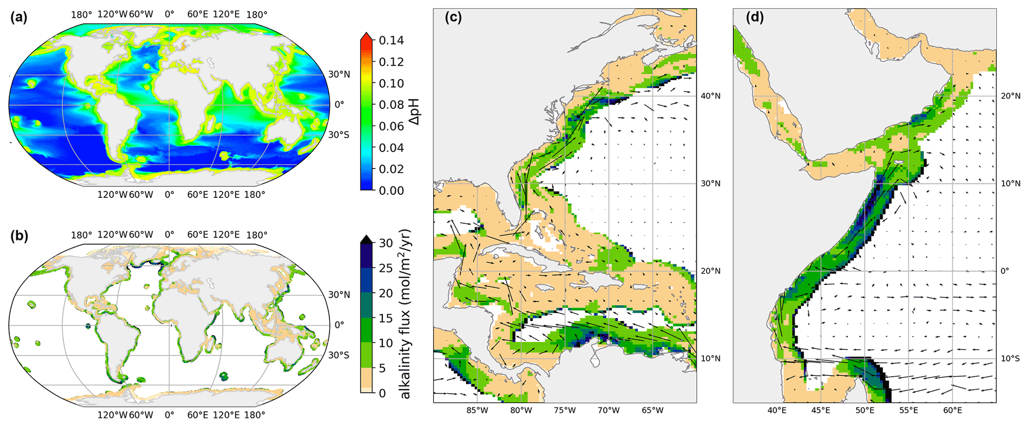
Figure 1Shown is a coastal injection in a strip 296 km wide, subject to ΔpH_tgt=0.1. All time-averages ran over 5–20 years. (a) Averaged pH change compared to a reference simulation with no added alkalinity. (b) Average alkalinity flux at each grid point from the coast. (c, d) Injection flux for two example regions. Annually averaged surface currents are overlaid as a vector field.

As expected, ΔpH or ΔΩ_Arag outside the injection grid cells is much lower and never exceeds the target value. However, the effect on adjacent areas outside of the injection grid points is variable and depends on the pattern of ocean currents that sweep alkalinity away from injection areas. For instance, western boundary currents carry the coastal excess alkalinity far out into the open ocean, so we see elevated changes in the North Atlantic and Indian oceans, even outside the injection areas.

For each injection pattern and chosen limit we can now obtain a global map of steady-state alkalinity flux (mol m⁻² yr⁻¹), which shows the variability of capacity for OAE (Fig. 1b, c and d). We note substantial variability on multiple scales. Firstly on a large scale, some coastal areas have a fundamentally greater capacity for distributing and neutralizing alkalinity flux than others (see also Fig. 2b). Large capacities are found around islands which sit in or near ocean currents, as those rapidly sweep the alkalinity away from near-coast areas. Examples include Kerguelen, Easter Island and Hawaii. Continental coasts which exhibit large capacities are found around South and East Africa, off the coast of Peru and Brazil, Southeast Australia and the west coast of Japan. Finally, an area of very large tolerance for alkalinity addition is found in the northern Atlantic. However, as will be shown later, this is due to downwelling and deep water formation, which is highly undesirable for OAE as the alkalinity cannot efficiently equilibrate with the atmosphere before being lost. Conversely inland seas and partially enclosed seas exhibit the smallest capacity for OAE, notably the Red Sea, the Mediterranean and the Baltic Sea. An interesting counterexample is the Gulf of Mexico and the Caribbean Sea which, owing to the traversing Gulf Stream, have significant capacity for OAE. We found no correlation between background pH and OAE rate, as the influence of local ventilation due to currents dominates the capacity for alkalinity addition.

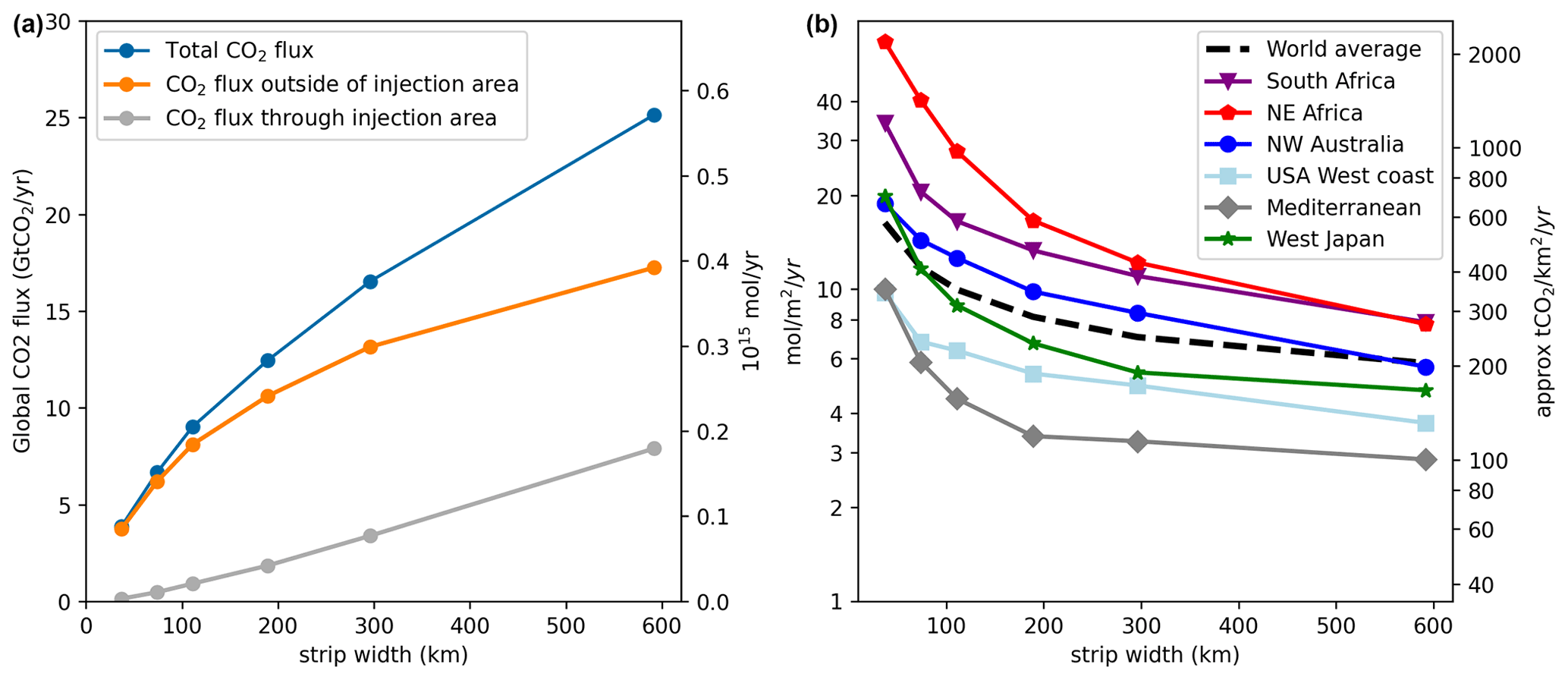
Figure 2(a) Total CO₂ flux (Gt CO₂ yr⁻¹), subject to ΔpH_tgt=0.1, broken down into flux through the injection area and outside of the injection area. (b) Dependence of the averaged injection flux (mol m⁻² yr⁻¹) on the width of the coastal injection strip for different coastal regions and strip widths. The black dashed line averages all coastal regions.

Download

As expected, the large scale patterns obtained by limiting ΔpH = 0.1 or ΔΩ_Arag=0.5 are very similar (Fig. S2) up to a linear factor and highly correlated on a per grid cell basis. This is consistent with the observation that OAE capacity is primarily influenced by local currents. However, we note that the fundamental sensitivities of pH and Ω_Arag with respect to Alk change quite differently from the Poles to the Equator. In particular, $\partial \mathrm{pH}/\partial \mathrm{Alk}$ decreases from $\sim \mathrm{2.6}\times {\mathrm{10}}^{\mathrm{3}}$ L mol⁻¹ at the poles to $\sim \mathrm{1.0}\times {\mathrm{10}}^{\mathrm{3}}$ L mol⁻¹ at the Equator, while $\partial \mathrm{\Omega }/\partial \mathrm{Alk}$ increases from $\sim \mathrm{7.6}\times {\mathrm{10}}^{\mathrm{3}}$ L mol⁻¹ at the Poles to $\sim \mathrm{11}\times {\mathrm{10}}^{\mathrm{3}}$ L mol⁻¹ at the Equator (computed from GLODAPv2, Lauvset et al., 2016; Olsen et al., 2017 data and pyCO2SYS; Humphreys et al., 2020; Lewis and Wallace, 1998). Furthermore, from the perspective of preventing precipitation due to excessive Ω_Arag, the available headroom is much smaller at tropical latitudes, where Ω_Arag is already close to 4, than near the poles where Ω_Arag is as low as 1–2 (Lauvset et al., 2016; Olsen et al., 2017). Thus, as our relative ΔΩ_Arag limit was set to 0.5, the OAE limits obtained here should be considered a lower bound with respect to calcite precipitation, i.e., polar regions could tolerate a much larger addition rate. For pH the actual ecologically tolerable limits will vary from coast to coast, and we do not attempt to anticipate them here. We note, however, that for our examined constraints (both of which are very conservative) a significant amount of negative emissions can be obtained even in very narrow coastal strips as the transport out to open sea is very efficient. This observation is consistent with prior work by Feng et al. (2017).

On a fine scale we find that the sustainable injection flux varies over 2–3 orders of magnitude between nearby grid points (Fig. S1) with a distribution that is approximately log-normal. The variance is even larger for thin injection strips (Fig. S1) and very large fluxes can be sustained in some locations if the net transport of alkalinity out of the strip is high enough. Depending on the prevailing currents, the highest injection rate can be found both on the outside and inside of the injection strip.

For all regions we observed that while widening the injection strip increases the total allowable rate of alkalinity injection, the increase is sublinear (Fig. 2a). Every additional unit of alkalinity added needs to be transported further offshore and the average injection rate decreases per unit area. This is consistent with the view that the majority of the neutralization of the added alkalinity by invading CO₂ occurs outside the injection strip and the local pH is primarily determined by the rate of transport of alkalinity into other areas (Burt et al., 2021). This is confirmed by integrating the total CO₂ flux over the injection strip and over the rest of the ocean surface, relative to the reference simulation. Figure 2a shows that especially for thin coastal injection strips, direct gas exchange through the strip surface accounts for only a minor component of the induced CO₂ uptake and the majority occurs outside of the injection areas. As the strip widens, however, this fraction significantly increases. Especially in regions with weak transport we observe that often a larger quantity of alkalinity can be added right at the border of the strip than in the middle, as alkalinity can dilute to bordering areas that are not directly receiving alkalinity (Fig. 3). Indeed, the largest alkalinity fluxes observed occur when the strip widths are very thin (Fig. S1). The consequence is that any particular coastal region can increase its capacity for injection by going further out to sea, but that there are diminishing returns of doing so, i.e., the increase in capacity is sublinear with width.

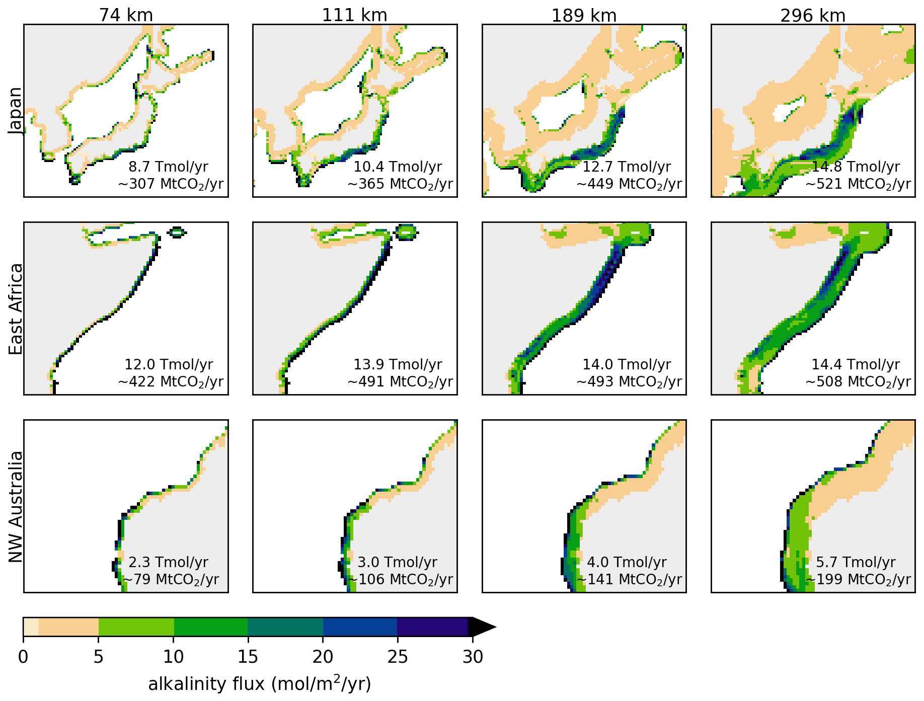
Figure 3Injection flux (mol m⁻² yr⁻¹) shown for different strip widths in 3 different regions (from top to bottom: Japan, East Africa and Northwest Australia). The inset text indicates the total alkalinity added per year in the shown area.

The influence of widening the injection area is also shown in detail for three regions in Fig. 3 and a larger number of regional details are included in the Supplement in Fig. S4. Widening strips allows more alkalinity to be added overall. However, saturation of near-coast areas occurs in most regions (especially evident in Northwest Australia). The largest injection flux is often found directly at the strip boundary, owing to easy diffusion out to open sea. However, it is not always the case that the highest injection flux occurs at the strip edge, as seen in the Japan and East Africa examples. These findings illustrate the highly non-local nature of the injection capacity.

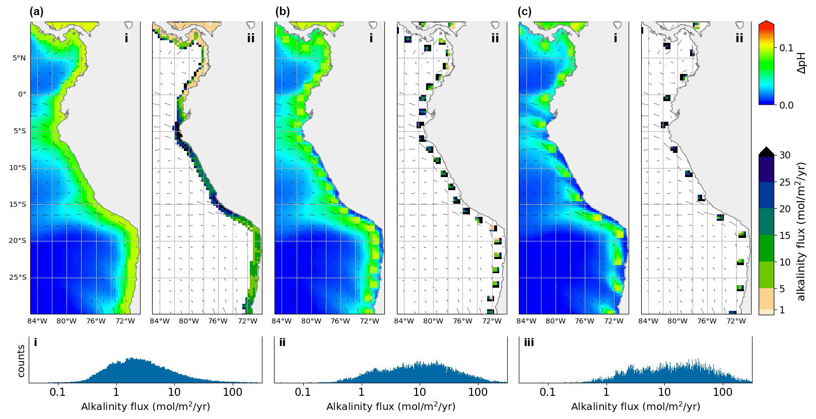
Figure 4Alkalinity enhancement in three different patterns, exemplified at the west coast of South America: (a) Injection in a contiguous strip. (b) Injection in 200 km separated patches. (c) Injection in 400 km separated patches. The total globally area-integrated OAE rate for the three injection patterns was (a) 336 Tmol yr⁻¹, (b) 312 Tmol yr⁻¹ and (c) 233 Tmol yr⁻¹, respectively. The sub panels show (i) time averaged pH change, (ii) alkalinity flux, (iii) distribution of alkalinity flux (globally).

In general we find that the sensitivity of pH and Ω_Arag at any given grid point is highly dependent on the surrounding pattern of injection. We conducted two additional experiments in which rather than a contiguous strip, injection occurred at discrete points placed either 200 or 400 km apart. At 200 km apart we observed much higher injection fluxes in each injection patch, but the total global injection flux barely changed (Fig. 4). Placing injection patches 400 km apart instead of 200 km apart did not further increase the sustainable flux in each injection patch, and reduced the overall injection capacity by 25 %. This suggests that at 200 km there is still significant cross-correlation between neighboring patches, which is apparent when looking at the pH changes observed: the pH impact bleeds into neighboring patches (Fig. 4b). At 400 km apart, however, there is much less interference between adjacent patches and the injection limits are simply dominated by local current patterns (Fig. 4c). These observations are consistent with prior work (Jones et al., 2012) which found a global median pCO₂ autocorrelation length of about 400 km. Thus in order to maximize any particular coastline's injection potential, injection areas should be placed at most 200–400 km apart; however, the exact optima will depend on the local current patterns. The location of ports, infrastructure, access to electricity and/or alkaline minerals will dictate the choice of locations. The correlation between neighboring injection locations has ramifications for the planning, monitoring and governance of different OAE projects, as they will affect each other in downstream coastal areas. For monitoring and verification purposes it will be impossible to disambiguate CO₂ drawdown caused by different OAE projects by measurement alone. Any plans to add alkalinity to the ocean will need to be simulated specifically, ideally with regionally optimized models, and take into account already occurring OAE projects nearby.

3.2 CO₂ uptake time scales

To measure localized CO₂ uptake time scales, we conducted a total of 17 pulse injections (as described in the methods section), placed near all major coastlines. We generally chose locations previously determined as areas of high alkalinity tolerance. Firstly, we observed a very large variety of CO₂ uptake time scales (Fig. 5) both in the short term (after 1 year) and in the medium term (after 10 years). After 1 year the molar uptake fraction ${\mathit{\eta }}_{{\mathrm{CO}}_{\mathrm{2}}}=\mathrm{\Delta }\mathrm{DIC}/\mathrm{\Delta }\mathrm{Alk}$ varied between 0.2 and 0.85 and after 10 years most locations resulted in an uptake fraction of 0.65–0.80 consistent with previous work (Tyka et al., 2022; Burt et al., 2021).

Figure 5CO₂ uptake relative to alkalinity addition (molar ratio ${\mathit{\eta }}_{{\mathrm{CO}}_{\mathrm{2}}}=\mathrm{\Delta }\mathrm{DIC}/\mathrm{\Delta }\mathrm{Alk}$) following pulse additions at 17 different locations. (a) Locations which equilibrate fast and reach close to the theoretical maximum of CO₂ uptake (∼0.8). (b) Locations which equilibrate fast but reach a lower plateau of relative CO₂ absorption (0.6–0.8) with slow further progression. (c) Locations with slow equilibration or significant loss of alkalinity to the deep. Note that in some cases despite the slower initial equilibration high uptake ratios can be eventually achieved.

Download

A typical behavior is observed, for example, when releasing alkalinity at the northern coast of Brazil (Fig. 6a). Here the alkalinity remains long enough at the surface to realize its full CO₂ uptake potential within 2–3 years. A number of other tested locations follow this general pattern and are efficient for OAE deployment (Fig. 5a). Here the equilibration follows roughly a single exponential relaxation.

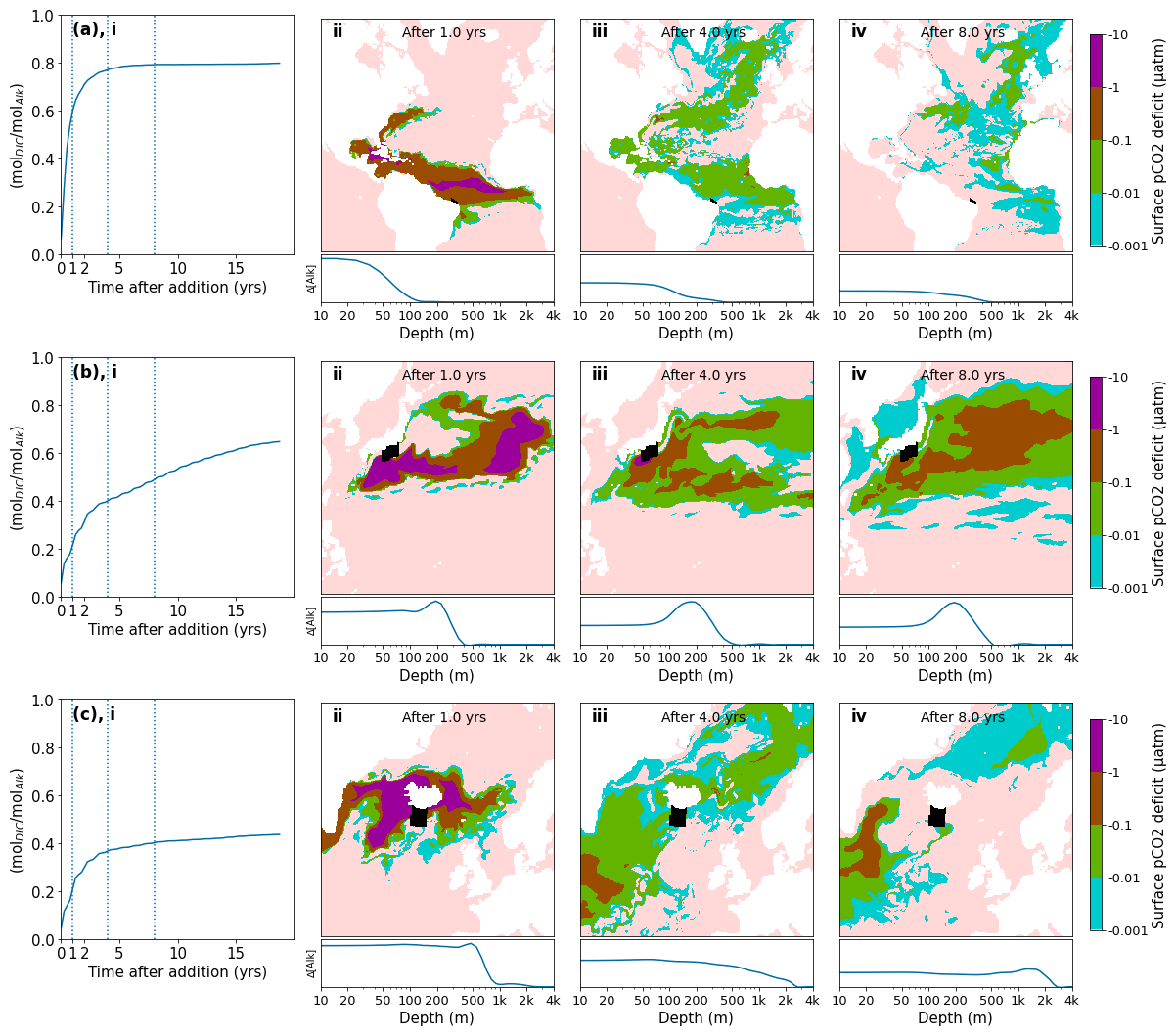
Figure 6Pulse additions of alkalinity in 3 representative locations: (a) Brazil, (b) Japan, (c) Iceland. (i) Excess quantity of CO₂ absorbed (relative to the reference simulation) over time following a 1 month pulse injection at various near coast locations, expressed as a molar fraction of the amount of alkalinity added (${\mathit{\eta }}_{{\mathrm{CO}}_{\mathrm{2}}}$). A significant variation of uptake time scales is observed, depending on the speed at which excess alkalinity is removed from surface layers, both in the short term and in the long term. (ii–iv) Spatial detail of surface pCO₂ deficit and depth residence of excess alkalinity for the same 3 locations shown in (i). The initial injection location is indicated by a black area. The surface pCO₂ deficit is plotted over time (note the log scale of the color map), indicating areas which are absorbing extra CO₂ (or emitting less CO₂) compared to the reference simulation. Below, the relative excess alkalinity is plotted against the depth of the water column (averaged over all lat/long grid points for each depth). Further locations are shown in detail in Fig. S5.

Another set of locations appear to lose a significant amount of alkalinity to deeper layers before atmospheric equilibration is achieved (Fig. 5b, c). For example, injection off the coast of Japan resulted in slow initial uptake as a portion of the alkalinity is quickly subducted (Fig. 6b). However, in the following decade remixing with surface waters gradually returns this alkalinity back towards the surface resulting in slow but steady CO₂ uptake (Fig. 6b). Other examples of this delayed CO₂ equilibration are shown in Fig. 5b. These locations exhibit a short mixed layer residence time and have a poor equilibration efficiency (Jones et al., 2014), but equilibration is eventually achieved in the following decades. Changes in surface pCO₂ and alkalinity will also potentially affect biological CO₂ uptake and calcification rates; however, these dependencies are not captured by the carbonate model used here (Dutkiewicz et al., 2005) and will need to be examined by future studies.

Finally, some extreme examples of poor long-term equilibration efficiency are found in areas of deep water formation, such as the northern Atlantic. Here a CO₂ uptake ratio of just over 0.4 is achieved and even after 20 years very little further progress is made (Fig. 6c). Around half of the added alkalinity is subducted very deep and will likely remain out of contact with the atmosphere until the global overturning circulation returns these waters to the surface, on the time scale of many hundreds of years. We did not examine the dependence of the time of year (all of our pulses occurred in January) nor were we able to conduct an exhaustive set of locations as was done previously with a coarser global circulation model (Tyka et al., 2022). We note that for all cases the alkalinity-induced CO₂ deficit spreads over a very large area within 1 year and a significant fraction of the CO₂ uptake occurs after the deficits have diluted to the sub-µatm range. This makes direct monitoring and verification of OAE extremely challenging and will likely need to rely on modeling and indirect experimental verification.

3.3 Alkalinity injection from ships

Other than potential ecological impacts on marine life intersecting the caustic release wake of an OAE ship, one concern is that a short Ω_Arag spike could induce precipitation of CaCO₃ (Renforth, 2012). Once nucleated, the CaCO₃ particles could continue to grow, even when the pH has returned to normal ocean levels (≈8.1) because the ocean is supersaturated with respect to calcite (Ω_Calc ≈ 2.5–6) and aragonite (Ω_Arag ≈ 1.5–4) (Lauvset et al., 2016; Olsen et al., 2017). While the nucleation of CaCO₃ is strongly inhibited by the presence of magnesium in seawater (Sun et al., 2015; Pan et al., 2021), the growth of existing crystals may not be (Moras et al., 2022; Hartmann et al., 2022). Only once the CaCO₃ particle has reached a size and density that causes it to sink would it stop removing alkalinity from the surface ocean. Thus, depending on the number of particles nucleated, the alkalinity removed from the surface ocean can be larger than the alkalinity added (Moras et al., 2022; Hartmann et al., 2022; Fuhr et al., 2022).

As the immediate dilution dynamics of alkalinity injected into the wake of a ship are far below the resolution of the ECCO LLC270 global circulation model, we examine this process analytically, as described in the methods section. The relevant time scales are compared in Fig. 7. The predicted pH and Ω_Arag as a function of time are shown in blue, based on the dilution formulas given by IMCO (1975) and Chou (1996).

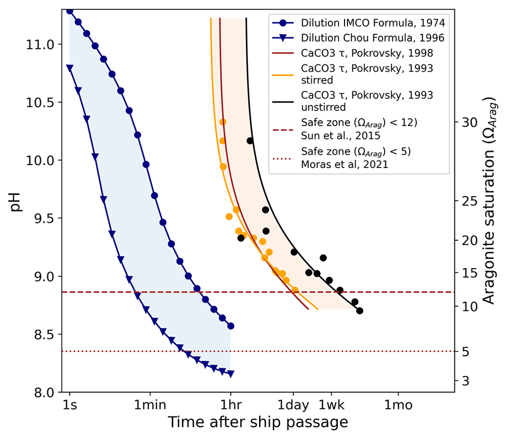
Figure 7The expected time evolution of pH (left scale) and Ω_Arag (right scale) due to dilution for alkalinity injection into a ship wake. Here we assume a large tanker (275 m long, 50 m wide, traveling at 6 m s⁻¹) releasing 1.0 M NaOH at a rate of 5 m³ s⁻¹. Ships of this size have a capacity of 100–200 kt of cargo which would take 6–12 h to discharge. Two previously published dilution models are shown in blue with a large variance apparent. For comparison, the time scales of homogeneous nucleation are also shown (yellow, brown and black). The dashed and dotted lines indicate the estimated Ω limits for precipitation. Despite the substantial uncertainty in the existing models, dilution can proceed at least 1–2 orders of magnitude faster than precipitation is expected to occur.

Download

Also shown are the homogeneous nucleation times of CaCO₃ for comparison. Several studies (Pokrovsky, 1994, 1998) have measured the homogeneous nucleation of CaCO₃ in seawater at different saturation states down to Ω_Arag=9. Three of these models are plotted in shades of orange and black in Fig. 7. Theoretical studies (Sun et al., 2015) suggest that for Mg : Ca ratios of 5.2, as found in seawater, no nucleation of aragonite occurs at all below Ω_Calc=18 (equivalent to Ω_Arag≈12), due to inhibition by magnesium. This is consistent with Morse and He (1993); however, time scales only up to a few hours were examined. Moras et al. (2022) suggested a safe limit of Ω_Arag=5 based on alkalinity addition using CaO. Figure 7 shows that ship-wake dilution proceeds at least one order of magnitude faster than the homogeneous nucleation time; thus, we can expect that CaCO₃ particles will not be induced to nucleate.

At the immediate injection site where the pH exceeds ∼ 9.5–10.0, the temporary precipitation of Mg(OH)₂ is expected, which redissolves readily upon dilution (Pokrovsky and Savenko, 1995) and buffers the pH against further increase (not accounted for in Fig. 7). The temporary reduction in the Mg : Ca ratio could make CaCO₃ nucleation more favorable, but the time spent in this state (<1 min) is likely still well below the required nucleation time.

3.4 Transport costs

Alkalinity prepared on land must be transported out to sea, which incurs costs. Having obtained maps of the sustainable rate of OAE in any given area, we can estimate the transport costs for each of our simulated scenarios as described in the methods section. Furthermore, the quantity of alkalinity per tonne depends on the molality of the material moved. For rock-based methods (Hangx and Spiers, 2009; Schuiling and de Boer, 2011; Renforth, 2012; Montserrat et al., 2017; Rigopoulos et al., 2018; Meysman and Montserrat, 2017), the molality of solid alkaline materials such as olivine is ∼ 25 mol kg⁻¹. For electrochemical alkalinity methods (House et al., 2007; Rau, 2009; Davies et al., 2018; Eisaman et al., 2018; de Lannoy et al., 2018; Digdaya et al., 2020) that produce alkaline liquids it will be closer to 1 mol kg⁻¹, depending on the industrial processes used and effort spent concentrating the alkaline solution. Figure 8 shows how the transportation costs are influenced by the total desired negative emissions (larger scale requires transport further offshore). For concentrated alkalinity (such as ground rocks) transport costs are not a major contributor to cost, consistent with prior work (Renforth, 2012). However, for dilute alkalinity, such as that obtained from electrochemical processes, transportation could become a significant contributor to the overall cost. A potential low-cost solution could be, for example, the near-coast precipitation (Thorsen et al., 2000; Davies et al., 2018; Sano et al., 2018) of Mg(OH)₂ with subsequent redissolution of the solid Mg(OH)₂ after transport out to sea. However, economic tradeoffs between the cost of concentrating the alkalinity and the cost of transportation will need to be made.

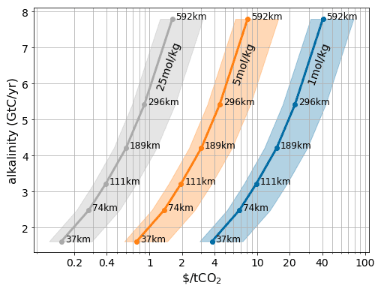
Figure 8Total carbon uptake potential for a variable alkalinity addition strategy that results in a maximal pH change of 0.1 (see Fig. 1 for an example). Carbon uptake is estimated at ${\mathit{\eta }}_{{\mathrm{CO}}_{\mathrm{2}}}=\mathrm{0.8}$. The strip widths necessary are indicated for each point. Shading denotes the shipping cost uncertainty, which ranges from USD 0.0016 to 0.004 per tonne per kilometer (Renforth, 2012).

Download