the Creative Commons Attribution 4.0 License.
the Creative Commons Attribution 4.0 License.
 | 18 Nov 2022
Temporal patterns and drivers of CO2 emission from dry sediments in a groyne field of a large river
Matthias Koschorreck
Klaus Holger Knorr
Lelaina Teichert
River sediments falling dry at low water levels are sources of CO2 to the atmosphere. While the general relevance of CO2 emissions from dry sediments has been acknowledged and some regulatory mechanisms have been identified, knowledge on mechanisms and temporal dynamics is still sparse. Using a combination of high-frequency measurements and two field campaigns we thus aimed to identify processes responsible for CO2 emissions and to assess temporal dynamics of CO2 emissions from dry sediments at a large German river.
CO2 emissions were largely driven by microbial respiration in the sediment. Observed CO2 fluxes could be explained by patterns and responses of sediment respiration rates measured in laboratory incubations. We exclude groundwater as a significant source of CO2 because the CO2 concentration in the groundwater was too low to explain CO2 fluxes. Furthermore, CO2 fluxes were not related to radon fluxes, which we used to trace groundwater-derived degassing of CO2.
CO2 emissions were strongly regulated by temperature resulting in large diurnal fluctuations of CO2 emissions with emissions peaking during the day. The diurnal temperature–CO2 flux relation exhibited a hysteresis which highlights the effect of transport processes in the sediment and makes it difficult to identify temperature dependence from simple linear regressions. The temperature response of CO2 flux and sediment respiration rates in laboratory incubations was identical. Also deeper sediment layers apparently contributed to CO2 emissions because the CO2 flux was correlated with the thickness of the unsaturated zone, resulting in CO2 fluxes increasing with distance to the local groundwater level and with distance to the river. Rain events lowered CO2 emissions from dry river sediments probably by blocking CO2 transport from deeper sediment layers to the atmosphere. Terrestrial vegetation growing on exposed sediments greatly increased respiratory sediment CO2 emissions. We conclude that the regulation of CO2 emissions from dry river sediments is complex. Diurnal measurements are mandatory and even CO2 uptake in the dark by phototrophic micro-organisms has to be considered when assessing the impact of dry sediments on CO2 emissions from rivers.
- Article
(2630 KB) -
Supplement
(645 KB) - BibTeX
- EndNote


1.1 CO2 emissions from dry river sediments – significance
Streams and rivers are known to play an important role in the global carbon cycle. The transport of continental carbon to the ocean is mainly regulated by rivers (Schlesinger and Melack, 1981). Moreover, carbon in rivers undergoes transformation processes and can be temporarily stored by means of sedimentation and photosynthesis or released due to biological respiration (Battin et al., 2009). One distinctive feature of rivers is their frequently changing water level. Climate change is expected to further increase the seasonal and the inter-annual variability of rivers and hydrological regimes (Bolpagni et al., 2019; Coppola et al., 2014). In Europe, more frequent and longer-lasting droughts are expected during summers, which lead to low water levels in streams and rivers (Spinoni et al., 2018). Consequently, previously submerged river sediment will be exposed to the atmosphere and influenced by drying (Steward et al., 2012). It has been shown that these exposed sediments can emit high amounts of CO2 (von Schiller et al., 2014) and may represent a globally relevant carbon source to the atmosphere (Marcé et al., 2019).
1.2 Regulation of CO2 emissions from dry sediments
While the relevance of CO2 emissions from dry river sediments has been acknowledged, only little is known about underlying mechanisms and temporal patterns. A recent study identified organic matter content and moisture as common drivers of CO2 emissions from dry aquatic sediments (Keller et al., 2020). However, high variability prevents the prediction of CO2 fluxes for particular sites. Case studies showed that CO2 emissions are affected by temperature (Doering et al., 2011), emergent vegetation (Bolpagni et al., 2017), organic matter (Palmia et al., 2021), water content (Martinsen et al., 2019), or the frequency of dry–wet cycles (Machado dos Santos Pinto et al., 2020). Although it is known that CO2 emission from dry sediment may change with time, existing studies are based on single or few measurements. Few studies addressed temporal variability of CO2 emissions, but nothing is yet known about short-term dynamics of greenhouse gas (GHG) emissions from dry aquatic sediments. Investigating temporal variability of CO2 fluxes should provide information about the potential sources of emitted CO2. Knowing sources of emitted CO2 from dry sediments is crucial to be able to model or scale up GHG emissions from these systems.
1.3 Possible sources of CO2
Carbon emissions from desiccated sediments derive from a number of possible biotic and abiotic sources (Marcé et al., 2019). Microbial respiration is known to contribute to CO2 emissions (Weise et al., 2016), similar to soil respiration. Organic matter originating from organic particle sedimentation may be mineralized to CO2 or CH4. It is typically observed that CH4 emissions from dry sediments are low, indicating that anaerobic mineralization plays a minor role (Marcé et al., 2019).
In contrast to respiration, abiotic processes are rarely taken into account as sources of CO2 (Rey, 2015). Yet, recent findings revealed a spatial variability of CO2 fluxes from dry river sediments with highest fluxes near to the river (Mallast et al., 2020). As a possible explanation, the authors hypothesized that at decreasing river water level a groundwater flow gradient towards the river would transport groundwater to the river (Peters et al., 2006). Groundwater is usually 10- to 100-fold super-saturated with CO2 (Macpherson, 2009). Near to the river the thickness of the unsaturated layer approaches zero and CO2 rich groundwater reaches the surface sediment where CO2 would eventually degas.
1.4 Aim of study
Given the uncertainty of the origin of CO2 emitted from dry river sediments, in this study we aimed to test the hypothesis of Mallast et al. (2020) that CO2 emissions from dry sediments of larger rivers are driven by groundwater degassing. If groundwater was a significant source of CO2, we hypothesize a only weak temperature dependence of CO2 emissions. We applied a combination of automatic high-frequency measurements and detailed studies using a variety of methods to identify the source of CO2 emissions from dry sediments at a large German river and to understand their temporal dynamics and drivers.
2.1 Study site
The study was conducted at the lowland part of the river Elbe, one of the largest rivers in central Europe with a discharge average of about 559 m3 s−1 at the city of Magdeburg (Weigold and Baborowski, 2009). Near Magdeburg, the middle Elbe can be characterized as a free-flowing, lowland river with comparable large floodplains, only regulated by groyne fields. Such groyne fields are the dominant shore type along the German part of the river (Bussmann et al., 2022).
Hence, seasonal water level fluctuations are shaping the different habitats alongside the river, ranging from alluvial forests and pastures to sandy beaches (Scholten et al., 2005). The study site is located near the farm “Apfelwerder” at river km 314 in between two groins and is characterized by a slight slope from the river to the adjoining pasture (52.038398∘ N, 11.715495∘ E). Groynes extended about 50 m into the river, and distance between groynes was 130±37 m. A sandy beach of about 2 to 5 m with sparse vegetation (Persicaria lapathifolia, Rorippa amphibia, Polygonum aviculare) could be found directly at the river, while the vegetation became denser with distance to the river (Fig. S1 in the Supplement).
2.2 High-frequency measurements
2.2.1 Automatic flux chambers, water table levels, and environmental data
To cover the temporal dynamics of CO2 fluxes three opaque automatic chambers (CFLUX-1 Automated Soil CO2 Flux System, PP systems, Amesbury, Massachusetts, USA), were installed (Fig. S1). The chambers measured CO2 fluxes once every hour. Each flux measurement lasted 5 min and between flux measurements the chambers were open for 55 min. CO2 fluxes were calculated from the linear increase of CO2 during a closure time of 5 min. Each chamber was equipped with a soil moisture and temperature probe (Stevens HydraProbe, Stevens Water Monitoring Systems, Portland, Oregon, USA). Due to fluctuating water levels over the summer of 2020 (Fig. 1), it was not possible to measure CO2 fluxes from the sediment continuously over the whole measurement period. The chambers were set up in the periods from 1 May to 10 June, from 3 to 6 August, and from 17 to 26 September; moreover, during deployment they needed to be moved occasionally. Automatic flux chamber data were discarded when the collar was flooded or the sand was washed away by waves, which resulted in CO2 concentrations fluctuating around ambient concentration. The final dataset contained 3128 flux measurements.
Because we did not know the exact elevation of our research site, we installed the chambers at defined heights relative to the gauge “Magdeburg Strombrücke” (located 13 km downstream of the study side, zero point of gauge = 39.885 m above mean sea level; ELWIS, 2020). Therefore, the distance to the river and the height over water level were determined once, along a transect. Out of these parameters, a slope was calculated and afterward used to position the automatic chambers in the field. Positions, where the automatic chambers were placed were related to gauge levels 75, 85, and 95 cm. In other words: when the gauge recorded a water level of, e.g., 75, a chamber at the “75 cm position” was located directly above the water line at our research site. The thickness of the unsaturated sediment was calculated as the difference between the height above zero gauge for each chamber and the actual river level. Weather data from the German Weather Service were obtained for the monitoring station Magdeburg 15 km from Apfelwerder (DWD, 2020).
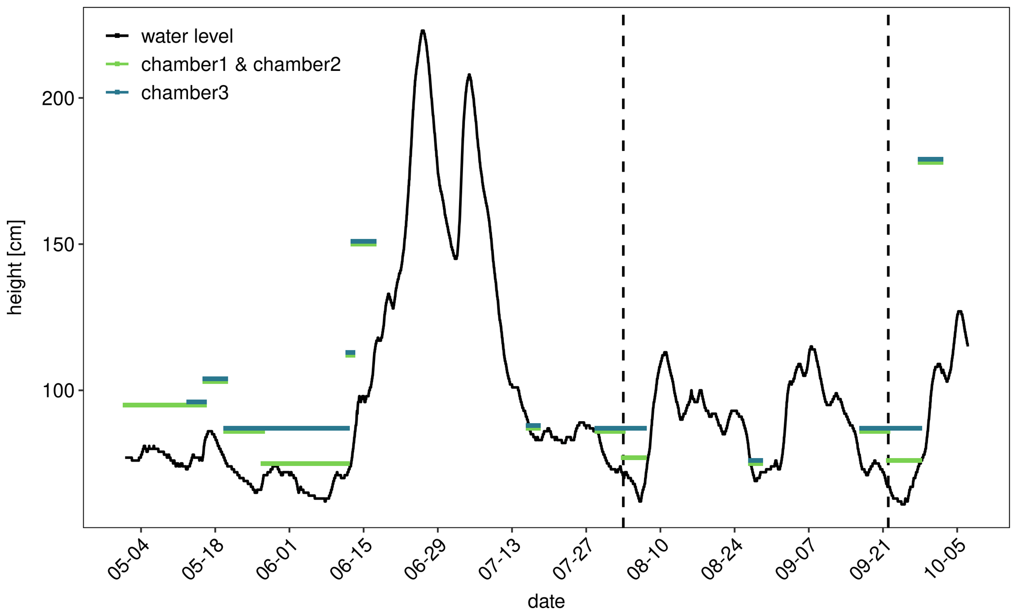
Figure 1Water level of the Elbe River at gauge Magdeburg Strombrücke (13 km downstream) in summer 2020. Colored lines indicate positioning of automatic flux chambers. For example a horizontal line at 95 cm means that a particular chamber was located at the water line when the gauge recorded a water level of 95 cm. Vertical dotted lines indicate intensive sampling campaigns.
2.2.2 High-resolution sediment respiration flux transects
To investigate spatial variability, between May and September, transects of sediment respiration were measured with a portable soil respiration system (EGM-5 Portable CO2 Gas Analyzer + soil respiration chamber, PP Systems, Amesbury, Massachusetts, USA) equipped with the same soil moisture and temperature probe as the automatic chambers. On each occasion 12 flux measurements along a 15 m long transect from the water upslope were recorded. The opaque chamber was placed on vegetation-free spots to make sure that sediment respiration was measured. At each measuring spot we took note whether plants were growing nearby.
2.3 Detailed sampling campaigns
To more closely investigate the mechanisms behind the CO2 flux, two intensive measurement campaigns were carried out on 4 August 2020 and 23 September 2020.
2.3.1 Manual chamber measurements
To quantify CO2 fluxes at different distances to the river and also check for CH4 emissions, manual chamber measurements were done in 1 m steps away from the flowing water, along a transect which was characterized by an uphill slope of ∼ 11.5 %. Collars (39 cm diameter) were installed at four sites along the transect a day in advance to minimize disturbance during measurements (Fig. S1b). For flux measurements, an opaque chamber (V=0.0239 m3, A=0.1195 m2) equipped with a pressure vent tube was placed on a collar. The concentrations in the chamber were measured every 30 s for ∼ 5 min with a multicomponent Fourier-transform infrared (FTIR) gas analyzer (DX4000, Gasmet Technologies GmbH, Helsinki, Finland). The FTIR gas analyzer continuously measures CO2, CH4, and nitrous oxide (N2O) with an accuracy of ±4 ppm CO2 and ±0.1 ppm CH4 and N2O (Gasmet Technologies GmbH 2018). Hence, the detection limit of the CO2 flux was ∼ 2 mmol m−2 d−1, while the CH4 flux was detectable if above 0.12 mmol m−2 d−1 and for N2O if above 0.2 mmol m−2 d−1. Fluxes were calculated from the linear increase of the respective gas mixing ratio (Gómez-Gener et al., 2015) with time using the R package glimmr (Keller, 2020).
2.3.2 Rn sediment efflux measurements
To assess groundwater degassing, 222Rn measurements were performed. The geogenic gas 222Rn is a commonly used natural tracer for groundwater influence in aquatic systems and is additionally known as a useful tool to trace the origins of CO2 (Cook and Herczeg, 2000). Therefore, 222Rn concentrations and fluxes were measured with a portable radon detector (RAD7 Radon Detector, DURRIDGE, Billerica, Massachusetts, USA) to determine the groundwater influence on CO2 fluxes from dry river sediments. The measurements of the RAD7 are based on electrostatic collection of alpha emitters with spectral analysis. Measuring with the “Normal” mode counts decays of both polonium decay products of 222Rn (218Po, 214Po). The counts were measured over 1 h and averaged, with a 1σ standard deviation and expresses as decays per second [Bq]. The measurement range lies between 4–750 000 Bq m−3 with an accuracy of ±5 %.
The 222Rn concentration in 300 mL samples from groundwater (2.3.3) and the river was measured with the Wat250 mode. In addition, soil 222Rn emissions were estimated with closed chamber measurements with the RAD7 over 3 h (one Rn measurement per hour). Assuming that groundwater is the main source of CO2 and that 222Rn moves at the same mass flow as CO2 (Megonigal et al., 2020), the same spatial dependence of CO2 and 222Rn fluxes would be expected in the case of groundwater being the major source of CO2. For this reason, 222Rn chamber measurements were performed simultaneously at two different positions: one with low and one with high CO2 flux. We used two chambers of different sizes and corrected 222Rn flux measurements [Bq m−3 d−1] for different chamber geometry by multiplying with the volume [m3] and dividing by the area [m2] of the chamber to get the 222Rn flux [Bq m−2 d−1].
2.3.3 Water + sediment sampling
For groundwater, sampling piezometers with a diameter of 2.7 cm and a length of 100 cm were installed next to each collar (Fig. S1b) a day before the sampling campaign.
To determine the thickness of the unsaturated zone, the water level in the piezometers was measured with an electric contact gauge. In situ parameters pH, conductivity, temperature, and O2 saturation were measured in the piezometers and the river with a multiparameter probe (WTW® MultiLine® Multi 3630 IDS, Xylem, Rye Brook, New York, USA). To analyze dissolved CO2 and CH4 concentrations, water samples were taken from the piezometers and the river using a syringe. Atmospheric air was added, with a headspace ratio of 1 : 1. After shaking for 2 min the headspace was transferred to 12 mL evacuated Exetainers (Labco Exetainers®, Labco Limited, Lampeter, UK) and stored till further analysis in the laboratory. Air samples were taken for headspace correction. Water samples for chemical analysis were collected in crimp vials without a headspace, stored at 4 ∘C, and later analyzed in the laboratory.
Soil samples from the 0–5 cm layer were taken around each collar for incubation experiments. Samples were filled into plastic bags, were stored at 4 ∘C, and analyzed in the laboratory within a week.
2.3.4 Potential CO2 production in laboratory incubations of sediment
Incubation experiments were set up to analyze the potential microbial respiration in dry river sediments under controlled conditions. For this purpose, fresh soil samples (25 g wet weight) taken along the transect were incubated in ∼ 130 mL vials in replicates of four at 19.5 ∘C. To determine the temperature dependence of microbial respiration, four replicate samples of 25 g were incubated at 4, 12, 19.5, 28, and 35 ∘C. From each vial, four to five gas samples were taken over an incubation period of 2 to 3 d by a Pressure-Lok® syringe (Pressure-Lok® glass syringe, Valco Instruments, Houston, Texas, USA) and analyzed by gas chromatography for CO2. Respiration rates were calculated from the linear increase of the CO2 content in the incubation vials divided by dry sediment weight.
To evaluate the temperature response of the microbial respiration in the sediment the Q10 temperature coefficient and the activation energy (Ea) was calculated (Dell et al., 2011). The activation energy was calculated as the slope of Arrhenius plots as described in Gillooly et al. (2001).
To compare respiration data from lab incubations to CO2 fluxes measured in the field rates, rates of respiration per gram dry weight [µmol g-dw d−1] were converted to fluxes by multiplying with sediment bulk density [g-dw cm−3] and the thickness of the reactive sediment layer which we assume to be equal to the thickness of the unsaturated zone [cm].
2.4 Analytics
CO2 and CH4 concentrations in gas samples were measured with a gas chromatograph (GC) (SRI 8610C, SRI Instruments Europe, Bad Honnef, Germany). The GC was equipped with a flame ionization detector and a methanizer which allowed for simultaneous measurement of CO2 and CH4 with an accuracy of <5 %. Dissolved gas concentrations were calculated using temperature-dependent Henry coefficients (UNESCO/IHA, 2010). Because the carbonate system in the headspace vial may change during headspace equilibration, CO2 concentrations were corrected for alkalinity as described in Koschorreck et al. (2021).
To analyze dissolved inorganic carbon (DIC), and dissolved organic carbon (DOC) water samples were filtered with a glass microfiber filter (Whatman GF/F). DIC and DOC concentrations were analyzed based on high-temperature oxidation and nondispersive infrared (NDIR) detection (DIMATOC® 2000, DIMATEC Analysentechnik, Essen, Germany). The alkalinity of the water samples was determined by titration with HCl to pH of 4.3. To determine the concentration of the cations K+, Na+, Ca2+, and Mg2+, the water samples were filtered with a 0.45 µm syringe filter, acidified with HNO3, and analyzed with an inductively coupled plasma optical emission spectrometer (ICP OES) (Optima 7300 DV, PerkinElmer, USA). The anion concentrations of SO and Cl− were measured with ion chromatography (Dionex ICS 6000, Thermo Fisher Scientific, Waltham, Massachusetts, USA).
Soil samples were analyzed to determine soil moisture content, bulk density, and organic matter from weight loss after drying for at least 2 d to constant weight at 105 ∘C and loss on ignition (LOI) at 550 ∘C, respectively. Sediment texture was determined by the FAO method (FAO, 2020).
2.5 Statistics
CO2 flux datasets from manual and automatic measurements were visually checked for normal distribution with Q–Q plots. Data were summarized by distance to the river and tested with a one-sample t test to determine if measured fluxes differed significantly from zero.
Spearman rank correlation was used to identify relationships between environmental variables and the observed CO2 flux and to identify the strength and direction of these relations (Leyer and Wesche, 2007). Additionally, representative periods and single days were selected from automatic measurements to analyze patterns hidden by the temporal variability of the data. The measured environmental variables of sediment temperature, sediment moisture, thickness of the unsaturated zone, organic matter content, and precipitation were used for correlation analysis. Water level and climate data were averaged over 1 h. Linear mixed-effects models (LMEs) were applied to predict the influence of the environmental variables on the CO2 flux at the study site for variables for which a linear relationship with the CO2 flux was presumed. Model selection was done by removing predictors and comparing conditional R2 values of different models. To apply simple linear regression models and LMEs, assumptions of normality and homoscedasticity were visually checked with diagnostic plots, including residuals vs. fitted and Q–Q plot. Flux data were log-transformed for LME analysis. Because of occasional small negative fluxes, we shifted all fluxes to positive values by adding 121 mmol m−2 d−1 prior to transformation (120 was the value of the largest negative flux). Statistical analysis was performed using R (R-Core-Team, 2016).
3.1 Long-term data
The river showed a typical summer discharge situation with a water level mostly below 1 m, interrupted by a high-discharge event at the end of June (Fig. 1). Considerable areas of dry sediments only emerged during 6 weeks in early summer and short periods in the first week of August and in September. CO2 fluxes measured during these periods showed high diurnal and seasonal fluctuations (Fig. 2). Fluxes fluctuated over 3 orders of magnitude between −120 and 1135 mmol m−2 d−1 with a median of 98 and a mean ± SD of 149±155 mmol m−2 d−1. Fluxes fluctuated in a narrow range below 200 mmol m−2 d−1 during the first phase of the investigations in May. Due to rising water level, on 17 May we moved the chambers higher up where we measured both higher fluxes and larger diurnal amplitudes. When the water level decreased after 20 May, we moved the chamber down to freshly emerged sediment. There, CO2 fluxes were similar to the fluxes measured 10 cm higher during the first half of May and tended to increase with increasing time since drying. Negative fluxes were observed in 193 out of 3128 flux measurements (= 6 % of all fluxes). Negative fluxes were observed especially during the beginning of the measurement period and at sites near to the water. Interestingly, negative fluxes nearly exclusively occurred during the day between 10:00 and 18:00, peaking in the afternoon (Fig. S2). Chambers installed closer to the water measured lower and less variable fluxes than chambers installed higher upslope.
Fluxes showed considerable short-term variability. Variability was not constant during the investigated period but especially high after June. Clear diurnal patterns were observed during the entire study but most pronounced in September.
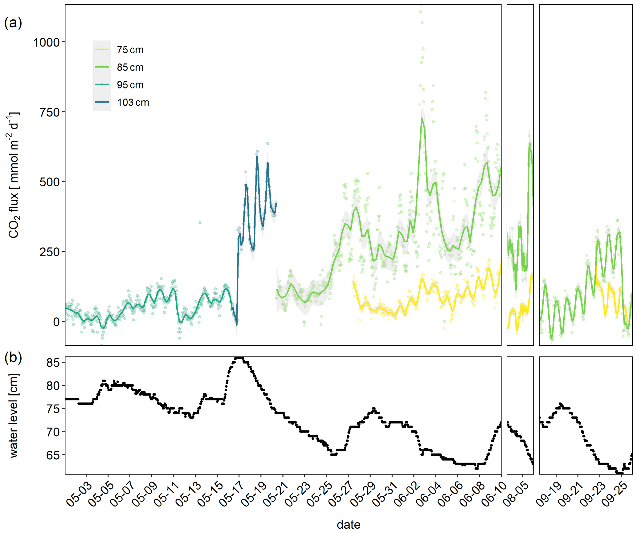
Figure 2CO2 fluxes in millimole per square meter per day measured with automatic chambers (a) and corresponding water level of the river measured 13 km downstream at the gauge Magdeburg Strombrücke (b). Colors indicate the elevation of the chambers. For example the 75 cm position means that the chamber was directly above the water line when the gauge reading was 75. Lines indicate smoothed data ± SD using locally estimated scatterplot smoothing (LOESS) smoother with a span 0.1. The grey areas indicate confidence intervals.
3.1.1 Regulatory factors: sediment moisture, temperature, water level, climate
The observed diurnal pattern with higher CO2 fluxes during the day suggested a temperature regulation of the flux. The CO2 flux was indeed weakly (Spearman p<0.05) correlated with the thickness of the unsaturated zone (R2=0.31), sediment temperature (R2=0.19, Fig. 3a), and moisture (), as well as precipitation (). A linear mixed-effects model with site where the chamber was placed as random factor and temperature and thickness of the unsaturated zone as fixed factors explained 0.61 % of the variability. Adding moisture did not further improve the LME (Table S1 in the Supplement).
The temperature response of the CO2 flux was not very clear, however, if all data were plotted together (Fig. 3a), but if data from single days were plotted, a clear pattern emerged (Figs. 3b and S3). The temperature response of the flux was affected by the time of day resulting in typical hysteresis curves. Warming during the day resulted in exponentially increasing fluxes. However, fluxes stayed high despite cooling which started in the afternoon – the temperature response of the flux was clearly delayed. From the CO2 flux–temperature relation (Fig. 3a) an activation energy of 0.56 eV (37 kJ mol−1) could be calculated which corresponds to a Q10 of 1.7 between 10 and 20 ∘C.
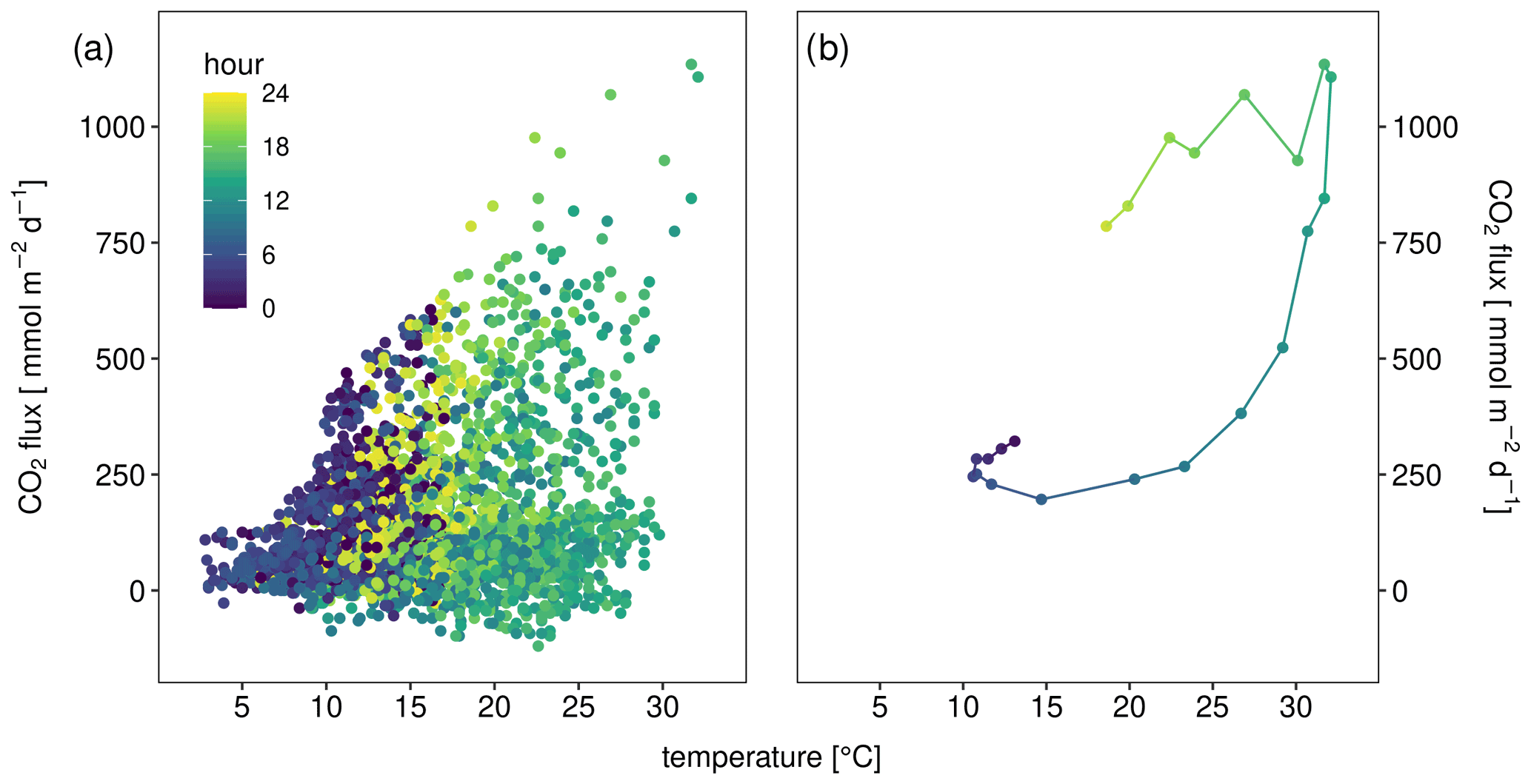
Figure 3CO2 flux in millimole per square meter per day (obtained from three automatic chambers) depending on sediment temperature of (a) all data and (b) only data from 2 June as an example for hysteretic response to temperature. Color indicates hour of measurement.
A closer look at data from a single week in September revealed how temperature, thickness of the unsaturated zone, and precipitation interacted in regulating the flux (Fig. 4). Temperature drove the very clear diurnal amplitude, but the absolute level of the flux was higher with increasing thickness of the unsaturated zone (which was accompanied by sediment drying). A single precipitation event on 25 September resulted in a sudden increase in sediment moisture which was accompanied by a clear drop of the CO2 flux. If only data for the period shown in Fig. 4 were considered, a linear model containing sediment temperature and moisture and the interaction between temperature and moisture explained 46 % of the variance.
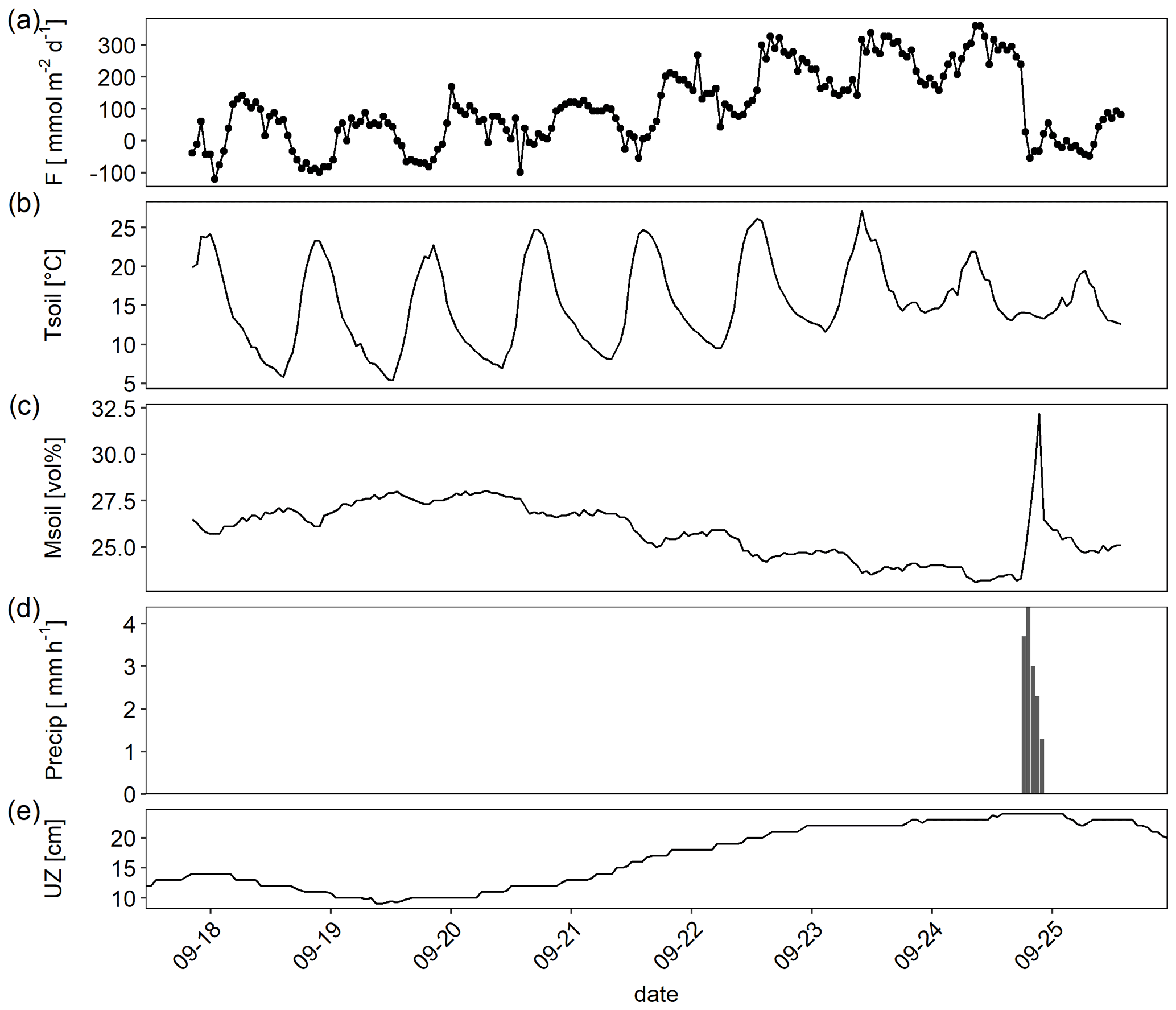
Figure 4Example high-frequency dataset showing (a) CO2 flux (F) measured by an automatic chambers, (b) sediment temperature (Tsoil; 0–5 cm depth), (c) sediment moisture (Msoil; 0–5 cm depth) (d) precipitation (Precip) recorded in hourly resolution, and (e) thickness of the unsaturated zone (UZ; distance between water table level and ground surface).
3.1.2 Spatial gradient of CO2 flux
Manual chamber measurements at different distances to the water revealed a spatial gradient of the CO2 flux. CO2 fluxes were lowest near to the water line where sediment moisture was highest (Fig. 5) and fluxes increased with distance to the water. This was also visible in the automatic chamber data when chambers were placed at different distances to the water (compare Fig. 2). The chamber which was placed nearer to the water recorded consistently lower fluxes. This is also consistent with the observed positive correlation between CO2 flux and the thickness of the unsaturated zone.

Figure 5CO2 flux (mmol m−2 d−1) as measured with a manual chamber (a) and sediment moisture (vol %) measured with a probe in 0–5 cm depth (b) depending on the distance to the water. The white lines indicates the plant line. The area below this line was free of vegetation. There were never plants inside chambers.
We also observed higher CO2 fluxes in the vicinity of plants. Plants were consistently found from about 3 m from the water uphill. Fluxes above this “plant line” (indicated by the white line in Fig. 5) tended to be higher than fluxes from the vegetation-free area nearer to the water.
In sum, our field-based measurements provide strong evidence that respiration in the sediment was the major driver of the observed CO2 flux. To further support this conclusion detailed investigations were carried out.
3.2 Detailed investigations
The sediment pore water was quite similar to river water with respect to electric conductivity and dissolved solutes including DIC (Table 1). The water level difference between the wells and the river was below the detection limit – the hydraulic gradient was virtually zero during our sampling campaigns. The shallow hydraulic gradient and the similar chemistry suggest a large influence of river water on the sediment pore water. In contrast, concentrations of dissolved gases were quite different with high concentrations of CO2 and CH4 and low concentrations of O2 in the pore water. Pore water concentrations of CO2 increased with distance to the river, while CH4 concentrations tended to be highest near to the river. In August, the river water was slightly undersaturated with respect to CO2. The sediment was poor in organic matter (LOI < 1 %) and texture was loamy sand. GHG emissions were dominated by CO2, while CH4 fluxes were low and N2O fluxes were always below the detection limit (Table 1).
Table 1Sediment, groundwater, and river water properties at the two sampling campaigns.
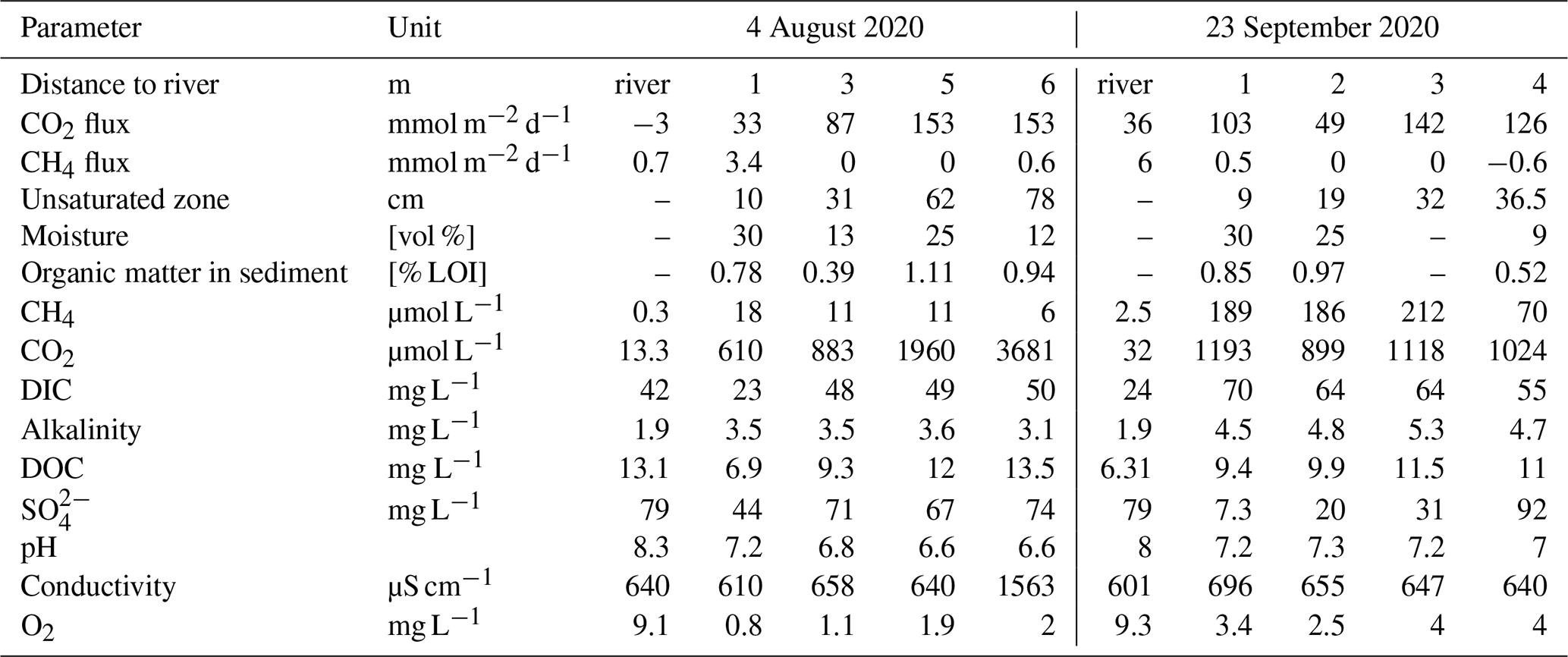
Diffusive fluxes from the river were calculated from concentrations using the gas transfer coefficient from Matoušů et al. (2019).
3.2.1 CO2 fluxes versus Rn fluxes
Groundwater contained more than 1 order of magnitude higher Rn concentrations than the river water (Table 2). As an indicator of groundwater degassing and possible evasion of CO2, we measured the flux of radon out of the sediment, assuming groundwater as a major source. Rn fluxes were higher in September than in August although the Rn concentration in the groundwater was similar in both months (Table 2). The flux of radon out of the sediment was, however, not much different at two different distances to the river, while the CO2 flux differed by about 1 order of magnitude between the same sites. If groundwater was the source of CO2, we would expect Rn fluxes to be related to CO2 evasion from groundwater; thus our data indicate that higher CO2 fluxes were not originating from groundwater.
Table 2Flux of radon measured as 222Rn increase in static chambers compared to CO2 flux measured in the same chambers and radon concentration determined as detected activity [Bq m−3] in the groundwater sampled in wells directly beside the chambers as well as in the river water (0 m distance).

3.2.2 Sediment respiration rates
To check whether the observed CO2 fluxes could be explained by microbial respiration in the sediment, laboratory incubations were carried out. Sediment respiration rates as measured in laboratory incubations were 0.9±0.45 µmol g−1 d−1 in August and 0.64 µmol g−1 d−1 in September with rates increasing with distance to the river. Potential CO2 fluxes calculated from these rates were similar or higher than CO2 fluxes measured in situ (Fig. 6). Thus, sediment respiration was high enough to explain the observed CO2 emissions.
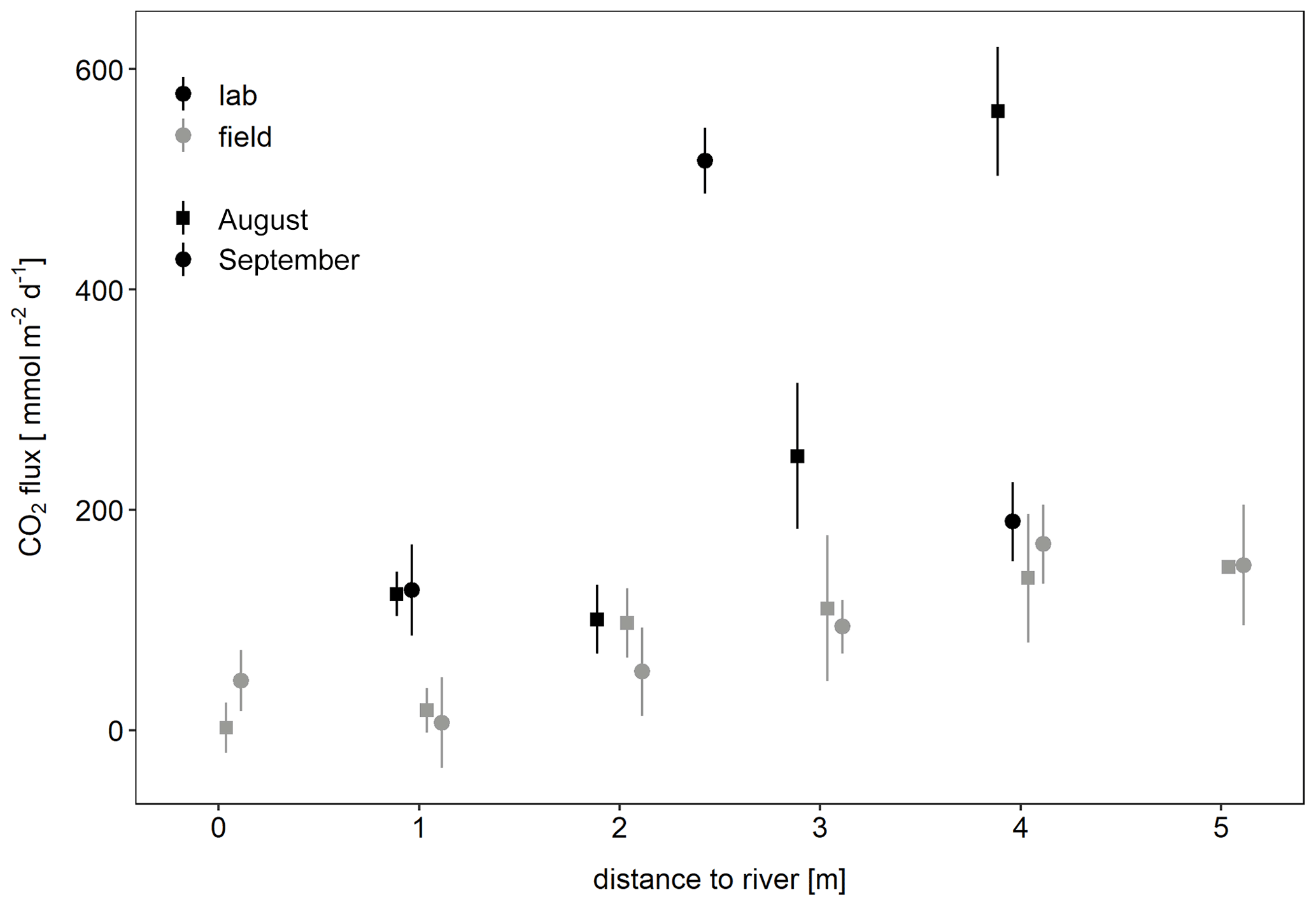
Figure 6Potential CO2 flux determined from laboratory incubations of sediment compared to in situ CO2 fluxes depending on distance to the river. Potential fluxes per unit area were calculated from sediment respiration rates [mmol g-dw−1 d−1], the thickness of the unsaturated zone [cm], and the bulk density of the sediment [g-dw cm−3].
3.2.3 Temperature dependence of sediment respiration
Sediment respiration increased exponentially with temperature (Fig. 7) resulting in a Q10 of 2.5. The calculated activation energy of 0.7 eV was similar to the activation energy calculated from the automatic chamber data. The comparison with the temperature response of the CO2 flux measured by the automatic chambers (line in Fig. 7) visualizes the similar temperature response of sediment respiration and in situ fluxes.
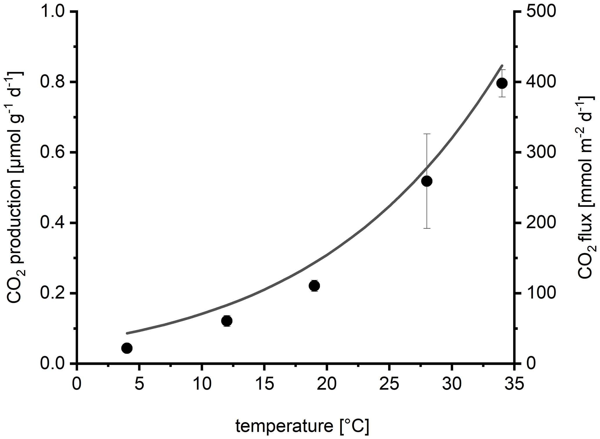
Figure 7Temperature dependence of sediment CO2 production (sediment respiration) in laboratory incubations depending on temperature (dots show mean ± SD of four replicates). For comparison, the line shows the average temperature response of the CO2 flux measured by automatic chambers, calculated by fitting the data from Fig. 3a to the Arrhenius equation.
4.1 Source of the CO2
Both our continuous data and detailed measurements show that the CO2 emitted from dry Elbe sediments originated from respiration in the sediment rather than from groundwater. This conclusion is consistently supported by numerous pieces of evidence:
-
The observed CO2 fluxes could be fully explained by sediment respiration measured in laboratory incubations. From soil respiration measurements, it is known that basal respiration as measured in laboratory incubations cannot be equivalent to soil CO2 emissions (Reichstein et al., 2000). A major difference between both methods is the exclusion of root respiration in bottle incubations which would lead to an underestimation of total soil respiration in root-free assays such as bottle incubations (Hanson et al., 2000). Thus, our sediment respiration rates measured in the laboratory are probably conservative estimates which even strengthens our argumentation.
-
The temperature response of the CO2 flux was very similar to the measured temperature response of sediment respiration and showed Q10 values typical for biological processes (Yvon-Durocher et al., 2012) and soil respiration (Hamdi et al., 2013). Potential evaporation on the other hand depends on radiation, vapor pressure, and wind speed (Penman, 1948) and only indirectly on surface temperature (Kidron and Kronenfeld, 2016). The temperature dependence of evaporation of soils depends on a complex interaction of texture and soil moisture and is not easy to predict (e.g., Federer, 2002). The observed temperature dependence provides strong evidence for respiration being the primary driver of the CO2 flux.
-
CO2 emissions increased with distance to the river. If groundwater was a major source of CO2 emissions, we would expect higher emissions at lower sediment elevation where groundwater potentially exfiltrated into the sediment. If there was a hydraulic groundwater gradient towards the river, this gradient should be steepest near to the river resulting in highest groundwater flux and potential outgassing near the river.
-
The CO2 flux was proportional to the volume of the unsaturated sediment. If CO2 originated from groundwater emissions, we would expect even a negative correlation because the transport of CO2 from the groundwater surface to the sediment surface should be inhibited by a larger unsaturated zone.
-
Higher CO2 emissions were not accompanied by higher Rn emissions. Groundwater typically contains high Rn concentrations, and Rn is a proven tracer to investigate groundwater input into surface waters (Perkins et al., 2015; Cook and Herczeg, 2000). We observed emission of Rn from the sediments indicating some influence of groundwater on the sediments. Rn emission at different distances from the river was identical. Thus, the thickness of the unsaturated sediment did not affect Rn emissions, showing that the anoxic zone itself was probably not a source of Rn. Soil Rn concentrations are known to be affected by meteorological and soil physical conditions (Asher-Bolinder et al., 1971). Similar Rn emissions, as observed in our study, are therefore an indication for similar sediment physical conditions. However, the magnitude of Rn emissions did not correspond to the magnitude of the CO2 emissions, indicating that the CO2 flux was independent from groundwater outgassing.
-
As we did not see hydraulic gradients indicative of larger groundwater inflow at our location of study, CO2 concentrations in the groundwater were too low to explain the observed CO2 flux. Groundwater degassing is relevant in situations when groundwater is pumped to the surface (Wood and Hyndman, 2017) or seeps into surface waters (Duvert et al., 2018). In rivers it might be relevant at seep sites which probably especially occur after fast water level drops and at extremely low water level.
Taken together our data consistently show that the observed CO2 emissions originated from respiratory CO2 production in the sediment. After having identified the primary source of CO2 we now look on the regulators of the magnitude of the CO2 emissions.
4.2 Regulation of CO2 emissions
Temperature is a master variable regulating several biogeochemical processes. Our temperature dependence (Q10 = 2.5, Ea = 0.7 eV) is in line with the temperature response of numerous ecological processes. A meta-analysis of 63 studies of temperature dependence of soil respiration revealed a mean Q10 of 2.6 (Hamdi et al., 2013). Diverse types of ecosystems have an activation energy of respiration of 0.65 eV (Yvon-Durocher et al., 2012) which is very similar to our study.
Temperature was an important regulator not only because of the temperature dependence of sediment respiration but also because the diurnal temperature amplitude was quite large. Sediment temperature not only ranged between 2.8 and 32 ∘C during the study period, but the complete temperature amplitude of about 20 ∘C could be observed during single days (Fig. 4). The large diurnal amplitude at these sites is favored by a lack of shadow and the fast heating of the sand which can lead to temperatures easily exceeding 40 ∘C (Mallast et al., 2020).
Although the temperature dependence of the CO2 flux is evident, it was not easily visible in flux versus temperature plots which show a large scatter (Fig. 3a). Only when looking at single days, a typical hysteresis pattern (Fig. 3b) became apparent. Such hysteresis curves have frequently been observed in high-frequency datasets of soil respiration (e.g., Riveros-Iregui et al., 2007). They originate from a phase lag between temperature and CO2 flux and can be explained by different transport of heat and CO2 in soils (Phillips et al., 2011) or by variable C supply from plants (Oikawa et al., 2014). The rotation direction as well as the shape of the ellipsoid depends on the vertical profile of temperature and activity in the soils as well as on the depth were soil temperature was measured. We measured temperature in 5 cm depth and obtained counterclockwise hysteresis which means that CO2 emissions were delayed relative to temperature measurements. A plausible explanation is that a large part of the CO2 was produced in deeper sediment layers where the daily temperature maximum was reached later. This is consistent with the observed positive correlation between CO2 flux and the thickness of the unsaturated zone. Theoretically the effect could also be caused by delayed outgassing of CO2 from deeper sediment layers due to CO2 transport limitation. However model calculations had shown that this mechanism was less relevant for shaping diurnal hysteresis in soils (Phillips et al., 2011). We quantified the delay by shifting flux and sediment–temperature data against each other (Fig. 8). By correlating the flux with the temperature 3 h before, we obtained the best linear correlation (R2=0.97) for the data in Fig. 3b. However, the time shift which produced the best linear fit differed between days (min = 0, max = 10, mean ± SD = 4.8±3.7 h) with a median of 4 h and no apparent differences between sites. Also the R2 of the best fit differed between 0.2 and 0.97. Thus, the hysteresis pattern obviously depended on the day of measurement and it is not possible to derive a general relation which then could be used to analyze temperature–flux relations of time-shift-corrected data.
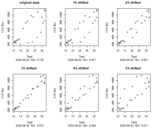
Figure 8Hysteresis loop for 2 June (same data as in Fig. 3b) with flux data shifted for various hours; 3 h shifted means that the flux at 10:00 local time (CEST) was correlated with the temperature at 07:00.
Wetting of dry soils typically triggers a pulse of CO2 production (Birch, 1958). However, in our case wetting events caused by rainfall reduced the CO2 flux as exemplified in Fig. 4. This shows that CO2 production in the sediment was not water limited and/or that the CO2 flux was rather transport limited when rainwater blocked gas-filled pores (Asher-Bolinder et al., 1971). At sediment moisture around 30 % in sandy sediments as measured in our study microbial activity in the sediment is probably not water stressed and consequently not stimulated by wetting. Thus, it is probable that the reduced CO2 flux after rain events was caused by physical blocking of soil pores. This is consistent with the observed long-term increase of the CO2 flux with decreasing moisture. Direct mechanistic dependence, however, is difficult to show because moisture also correlates with the thickness of the unsaturated zone (water level of the river relative to the sediment surface). This is why adding moisture to our mixed model only marginally increased the predictive power of the statistical model.
The thickness of the unsaturated zone was a strong predictor of the CO2 flux. The entire unsaturated zone obviously contributed to the CO2 flux. This is plausible because the intermediate sediment moisture both favored microbial processes and enabled gas exchange through gas-filled pores. This may also explain high CO2 fluxes in situations with extremely high sediment surface temperature (Mallast et al., 2020). Even if under such conditions CO2 production is inhibited at the surface, respiration in deeper layers may maintain high CO2 emissions.
The occurrence of vegetation, although excluded from our chamber measurements and restricted to the vicinity of the chambers, obviously is a game changer, largely stimulating sediment CO2 emissions. From our data we cannot fully distinguish whether higher fluxes near plants were caused by the plants or only by distance to the water (which is equivalent to the thickness of the unsaturated zone). However, the thickness of the unsaturated zone increased continuously, while the plant line represents a sudden change of conditions. Our data show a consistent high CO2 flux above the plant line. It is known that root respiration may contribute about 50 % to soil respiration (Hanson et al., 2000) and soil respiration is typically correlated with root biomass (Tufekcioglu et al., 2001). Thus, as we did not use trenched collars to exclude roots from chamber fluxes, it is highly probable that plants contributed to the elevated CO2 emissions through root respiration or provision of root exudates above the plant line. Higher sediment CO2 emissions, however, do not mean net CO2 emissions from the ecosystem since the vegetation growing on the dry sediments also fixes carbon and can even turn exposed sediments into a carbon sink (Bolpagni et al., 2017). To assess the effect of emerging vegetation on the overall carbon cycle of dry sediments, other methods like plant biomass determination or flux measurements including photosynthesis in transparent chambers are necessary.
4.3 CO2 uptake by the sediment
We frequently observed CO2 uptake by the sediment, although there were no plants and no light in our chamber. This is known from other studies and has been attributed to inorganic processes (Ma et al., 2013; Marcé et al., 2019). In our case the observed CO2 uptake could also be explained by the interaction of the sediment with river water. During May and June the river was undersaturated with CO2 (Fig. S4). The groundwater chemistry data show a gradient of concentrations increasing with distance to the river. This shows that the sediment pore water near to the river was affected by river water. Interestingly, negative fluxes were nearly exclusively observed during the daylight hours. A plausible explanation would be that ship-induced wave action might have triggered occasional river water intrusion and CO2 uptake by the sediment (Hofmann et al., 2010). This mechanism, however, cannot explain negative fluxes in September when the river was oversaturated with CO2 (Fig. S4).
Dark CO2 uptake could theoretically be caused by chemoautotrophic micro-organisms like nitrifiers. However, chemoautotrophic CO2 uptake should not be stimulated by light and is thus not consistent with our observation of nearly exclusive CO2 uptake during the day.
A straightforward explanation for negative CO2 fluxes during the day is CO2 uptake by phototrophic organisms. Algae and cyanobacteria are known to have active carbon concentrating mechanisms (CCMs) which allow CO2 uptake also in the dark (Giordano et al., 2005). Phototrophs living at the surface of dry sediments are facing a harsh environment with high salinity in thin water films covering particles and high irradiation and temperature – all factors favoring the activation of CCMs (Beardall and Giordano, 2002). Dark CO2 uptake is a common observation in 14CO2 uptake measurements and known to depend on pre-darkness light conditions (Legendre et al., 1983). In pure cultures, it has been shown that CO2 uptake by algae may proceed for more than an hour in darkness (Goldman and Dennett, 1986; Ohmori et al., 1984). Thus, it is highly plausible that the observed CO2 uptake by dry sediments was caused by photosynthetic algae and/or cyanobacteria. Future studies including chlorophyll analysis of sediments or the application of specific inhibitors may clarify the mechanism behind CO2 uptake in exposed river sediments.
4.4 Implications
Photosynthetic uptake of CO2 in the dark would have consequences for the interpretation of dark chamber measurements. If a chamber is placed on the sediment, photosynthetic CO2 uptake may proceed for an unknown period of time. The fact that no net uptake was observed in the night shows that the capability of dark CO2 uptake could not be sustained for periods longer than 1 h, which is consistent with pure culture observations (Goldman and Dennett, 1986). However, flux measurements are usually performed within a few minutes making it highly probable that they include eventual photosynthetic CO2 uptake. Comparison of transparent and opaque chamber measurements are sometimes used to detect photosynthesis of algae. Our results imply that such interpretation have to be treated with care because photosynthetic CO2 uptake may proceed during dark flux measurements.
Our median CO2 flux of 98 mmol m−2 d−1 would result in annual emissions of 429 g C m−2 yr−1 which is in the range of fluxes typical for temperate ecosystems (Doering et al., 2011) and similar to fluxes reported for dry Elbe sediments (Mallast et al., 2020) but high compared to the gravel bed of an alpine river (38 mmol m−2 d−1, Doering et al., 2011), and low compared to exposed sediments of Mediterranean streams (781 mmol m−2 d−1, Gómez-Gener et al., 2016). Although our observations thus fit the reported range, these differences as well as the large variation of fluxes observed in our high-frequency measurements (−120 to 1135 mmol m−2 d−1 – this range is larger than the range of typical fluxes for all kinds of terrestrial ecosystems as compiled by Doering et al., 2011) imply that care must be taken when upscaling fluxes not only for certain ecosystems but also for larger scales.
The observed hysteresis obscures flux–temperature relations if measurements were only performed at one time during the day. Thus, temperature regulation of dry sediment CO2 emissions might be more relevant and more complex than identified in a recent study (Keller et al., 2020).
Our high-frequency measurements show that standard measuring protocols are probably underestimating CO2 emissions from dry sediments because high fluxes in the night resulting from a delayed temperature response are not considered. The median flux measured between normal working hours (08:00–18:00) was 87 mmol m−2 d−1 compared to 98 mmol m2 d−1 if all data were considered. Thus, only measuring during daytime would lead to a flux underestimation of 11 %. We therefore recommend to assess temporal shifts in flux–temperature responses in order to obtain better estimates for upscaling based on a representative choice of flux data.
Our results are partly contradicting results from Mallast et al. (2020) who observed highest CO2 emissions near to the waterline. The two studies, however, are not directly comparable because the previous study by Mallast et al. (2020) was carried out under extreme drought conditions. Under such conditions, deeper lying sediments, which tend to be higher in organic matter and less sandy, were exposed to the atmosphere. Such conditions should favor CO2 emissions (Keller et al., 2020). Furthermore the very dry conditions (<10 % sediment moisture) under the extreme drought might have inhibited microbial processes in the sandy sediment. While the drivers of CO2 emissions from dry sediments are known, their complex interaction makes it difficult to predict CO2 emissions under a given situation.
The observed relation between CO2 flux and distance to the river, however, might facilitate upscaling of CO2 emissions from dry river sediments. The width of the dry sediment zone can be extracted from satellite images or aerial photographs. The observed consistent spatial pattern also implies that the CO2 flux was probably not much affected by time after exposure. Thus, combining few diurnal datasets of CO2 flux and lateral transects with seasonal data of the width of the dry sediments zone along a river is a promising approach to quantify total CO2 emissions from such systems.
We could clearly show that CO2 emissions from dry river sediments under the given conditions here were primarily driven by respiration in the sediment. Thus, existing knowledge about soil respiration might also apply to dry river sediments.
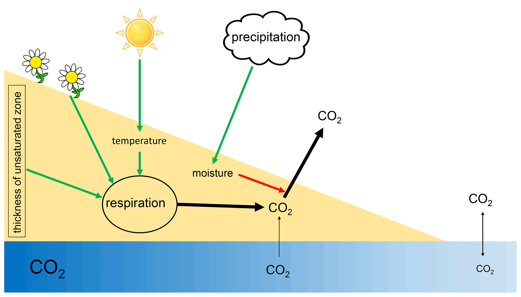
Figure 9Scheme of processes and drivers of CO2 fluxes from dry river sediments. Green arrows indicate positive effects; red arrows indicate negative effects.
We could further show that CO2 emissions were regulated by temperature and the thickness of the unsaturated zone (Fig. 8). The observed hysteresis effect clearly shows that simple correlations between environmental parameters and CO2 emissions from sediments may be too simplistic to study regulatory mechanisms. Positively spoken the analysis of such hysteresis relations may allow conclusions about underlying mechanisms (Musolff et al., 2021).
Our data show that the occurrence of terrestrial vegetation has a large and not yet assessed impact on the carbon cycle of dry sediments. To assess the effect of vegetation, not only ecosystem production but also the fate of plan biomass upon re-flooding has to be quantified. While it is clear that CO2 emissions from dry river sediments are relevant, the exact quantification of the effect of low river levels on the river carbon cycle remains challenging. Short-term temporal variation is very high and probably equally relevant as seasonal variability. Any attempt to quantify annual GHG emissions or the relevance of dry river sediments for carbon cycling needs to address temporal dynamics of CO2 emissions from dry river sediments.
The high-frequency dataset is supplied as a Supplement.
The supplement related to this article is available online at: https://doi.org/10.5194/bg-19-5221-2022-supplement.
MK initiated the study and prepared the manuscript with contributions from all co-authors. LT and MK performed measurements. All authors planned measurements and discussed the results.
The contact author has declared that none of the authors has any competing interests.
Publisher’s note: Copernicus Publications remains neutral with regard to jurisdictional claims in published maps and institutional affiliations.
Thanks to Martin Wieprecht for his excellent help during fieldwork and to Ulrike Berning-Mader and Corinna Völkner for their instructions and help in the laboratory of the University of Münster and UFZ. Thanks to Christian Wilhelm for advice regarding dark CO2 fixation, Bertram Boehrer for discussion and Peifang Leng for help using R.
This work was supported by funding from the Helmholtz Association in the
framework of Modular Observation Solutions for Earth Systems (MOSES).
The article processing charges for this open-access publication were covered by the Helmholtz Centre for Environmental Research – UFZ.
This paper was edited by Gabriel Singer and reviewed by Kenneth Thorø Martinsen and one anonymous referee.
Asher-Bolinder, S., Owen, D. E., and Schumann, R. R.: A preliminary evaluation of environmental factors influencing day-to-day and seasonal soil-gas radon concentrations, in: Field Studies of radon in rocks, soils, and water, edited by: Gundersen, L. C. S. and Wanty, R. B., US Geological Survey, Washingtom DC, ISBN 9781003070177, 1971.
Battin, T. J., Luyssaert, S., Kaplan, L. A., Aufdenkampe, A. K., Richter, A., and Tranvik, L. J.: The boundless carbon cycle, Nat. Geosci., 2, 598–600, https://doi.org/10.1038/ngeo618, 2009.
Beardall, J. and Giordano, M.: Ecological implications of microalgal and cyanobacterial CO2 concentrating mechanisms, and their regulation, Funct. Plant Biol., 29, 335–347, https://doi.org/10.1071/PP01195, 2002.
Birch, H. F.: The effect of soil drying on humus decomposition and nitrogen availability, Plant Soil, 10, 9–31, https://doi.org/10.1007/bf01343734, 1958.
Bolpagni, R., Folegot, S., Laini, A., and Bartoli, M.: Role of ephemeral vegetation of emerging river bottoms in modulating CO2 exchanges across a temperate large lowland river stretch, Aquat. Sci., 79, 149–158, https://doi.org/10.1007/s00027-016-0486-z, 2017.
Bolpagni, R., Laini, A., Mutti, T., Viaroli, P., and Bartoli, M.: Connectivity and habitat typology drive CO2 and CH4 fluxes across land–water interfaces in lowland rivers, Ecohydrology, 12, e2036, https://doi.org/10.1002/eco.2036, 2019.
Bussmann, I., Koedel, U., Schütze, C., Kamjunke, N., and Koschorreck, M.: Spatial Variability and Hotspots of Methane Concentrations in a Large Temperate River, Front. Env. Sci.-Switz., 10, 833936, https://doi.org/10.3389/fenvs.2022.833936, 2022.
Cook, P. G. and Herczeg, A. L.: Environmental Tracers in Subsurface Hydrology, Springer, Boston, 529 pp., ISBN 9780792377078, 2000.
Coppola, E., Verdecchia, M., Giorgi, F., Colaiuda, V., Tomassetti, B., and Lombardi, A.: Changing hydrological conditions in the Po basin under global warming, Sci. Total Environ., 493, 1183–1196, https://doi.org/10.1016/j.scitotenv.2014.03.003, 2014.
Dell, A. I., Pawar, S., and Savage, V. M.: Systematic variation in the temperature dependence of physiological and ecological traits, P. Natl. Acad. Sci. USA, 108, 10591–10596, https://doi.org/10.1073/pnas.1015178108, 2011.
Doering, M., Uehlinger, U., Ackermann, T., Woodtli, M., and Tockner, K.: Spatiotemporal heterogeneity of soil and sediment respiration in a river-floodplain mosaic (Tagliamento, NE Italy), Freshwater Biol., 56, 1297–1311, https://doi.org/10.1111/j.1365-2427.2011.02569.x, 2011.
Duvert, C., Butman, D. E., Marx, A., Ribolzi, O., and Hutley, L. B.: CO2 evasion along streams driven by groundwater inputs and geomorphic controls, Nat. Geosci., 11, 813–818, https://doi.org/10.1038/s41561-018-0245-y, 2018.
DWD: Datenbasis, Einzelwerte gemittelt, DWD [data set], ftp://opendata.dwd.de/climate_environment/CDC/observations_germany/climate/hourly/, last access: 3 March 2020.
ELWIS: Wasserstände & Vorhersagen an schifffahrtsrelevanten Pegeln, Pegel Magdeburg-Strombrücke, ELWIS [data set], https://www.elwis.de/DE/dynamisch/gewaesserkunde/wasserstaende/index.php?target=1&pegelId=ccccb57f-a2f9-4183-ae88-5710d3afaefd, last access: 11 August 2020.
FAO: Soil testing methods: global soil doctors programme – a farmer to farmer training programme, Soil testing methods manual, FAO (Food and Agriculture Organization of the United Nations), ISBN 9789251311950, 2020.
Federer, C. A.: BROOK 90: A simulation model for evaporation, soil water, and streamflow, GitHub, https://github.com/rkronen/Brook90_R (last access: 15 November 2022), 2002.
Gillooly, J. F., Brown, J. H., West, G. B., Savage, V. M., and Charnov, E. L.: Effects of size and temperature on metabolic rate, Science, 293, 2248–2251, https://doi.org/10.1126/science.1061967, 2001.
Giordano, M., Beardall, J., and Raven, J. A.: CO2 concentrating mechanisms in algae: Mechanisms, environmental modulation, and evolution, Annu. Rev. Plant Biol., 56, 99–131, https://doi.org/10.1146/annurev.arplant.56.032604.144052, 2005.
Goldman, J. C. and Dennett, M. R.: Dark CO2 Uptake by the Diatom Chaetoceros-Simples in Response to Nitrogen Pulsing, Mar. Biol., 90, 493–500, https://doi.org/10.1007/Bf00409269, 1986.
Gómez-Gener, L., Obrador, B., von Schiller, D., Marce, R., Casas-Ruiz, J. P., Proia, L., Acuna, V., Catalan, N., Munoz, I., and Koschorreck, M.: Hot spots for carbon emissions from Mediterranean fluvial networks during summer drought, Biogeochemistry, 125, 409–426, https://doi.org/10.1007/s10533-015-0139-7, 2015.
Gómez-Gener, L., Obrador, B., Marcé, R., Acuña, V., Catalán, N., Casas-Ruiz, J. P., Sabater, S., Muñoz, I., and Schiller, D.: When Water Vanishes: Magnitude and Regulation of Carbon Dioxide Emissions from Dry Temporary Streams, Ecosystems, 19, 710–723, https://doi.org/10.1007/s10021-016-9963-4, 2016.
Hamdi, S., Moyano, F., Sall, S., Bernoux, M., and Chevallier, T.: Synthesis analysis of the temperature sensitivity of soil respiration from laboratory studies in relation to incubation methods and soil conditions, Soil Biol. Biochem., 58, 115–126, https://doi.org/10.1016/j.soilbio.2012.11.012, 2013.
Hanson, P. J., Edwards, N. T., Garten, C. T., and Andrews, J. A.: Separating root and soil microbial contributions to soil respiration: A review of methods and observations, Biogeochemistry, 48, 115–146, https://doi.org/10.1023/A:1006244819642, 2000.
Hofmann, H., Federwisch, L., and Peeters, F.: Wave-induced release of methane: Littoral zones as a source of methane in lakes, Limnol. Oceanogr., 55, 1990–2000, https://doi.org/10.4319/lo.2010.55.5.1990, 2010.
Keller, P. S.: glimmr: Compute gasfluxes with R, Gas Fluxes and Dynamic Chamber Measurements, GitHub [code], https://github.com/tekknosol/glimmr (last access: 15 November 2022), 2020.
Keller, P. S., Catalán, N., von Schiller, D., Grossart, H. P., Koschorreck, M., Obrador, B., Frassl, M. A., Karakaya, N., Barros, N., Howitt, J. A., Mendoza-Lera, C., Pastor, A., Flaim, G., Aben, R., Riis, T., Arce, M. I., Onandia, G., Paranaíba, J. R., Linkhorst, A., del Campo, R., Amado, A. M., Cauvy-Fraunié, S., Brothers, S., Condon, J., Mendonça, R. F., Reverey, F., Rõõm, E. I., Datry, T., Roland, F., Laas, A., Obertegger, U., Park, J. H., Wang, H., Kosten, S., Gómez, R., Feijoó, C., Elosegi, A., Sánchez-Montoya, M. M., Finlayson, C. M., Melita, M., Oliveira Junior, E. S., Muniz, C. C., Gómez-Gener, L., Leigh, C., Zhang, Q., and Marcé, R.: Global CO2 emissions from dry inland waters share common drivers across ecosystems, Nat. Commun., 11, 2126, https://doi.org/10.1038/s41467-020-15929-y, 2020.
Kidron, G. J. and Kronenfeld, R.: Temperature rise severely affects pan and soil evaporation in the Negev Desert, Ecohydrology, 9, 1130–1138, https://doi.org/10.1002/eco.1701, 2016.
Koschorreck, M., Prairie, Y. T., Kim, J., and Marcé, R.: Technical note: CO2 is not like CH4 – limits of and corrections to the headspace method to analyse pCO2 in fresh water, Biogeosciences, 18, 1619–1627, https://doi.org/10.5194/bg-18-1619-2021, 2021.
Legendre, L., Demers, S., Yentsch, C. M., and Yentsch, C. S.: The C-14 Method – Patterns of Dark CO2 Fixation and DCMU Correction to Replace the Dark Bottle, Limnol. Oceanogr., 28, 996–1003, https://doi.org/10.4319/lo.1983.28.5.0996, 1983.
Leyer, I. and Wesche, K.: Multivariate Statistik in der Ökologie. Eine Einführung, Springer, Berlin, https://doi.org/10.1007/978-3-540-37706-1, 2007.
Ma, J., Wang, Z.-Y., Stevenson, B. A., Zheng, X.-J., and Li, Y.: An inorganic CO2 diffusion and dissolution process explains negative CO2 fluxes in saline/alkaline soils, Sci. Rep.-UK, 3, 2025, https://doi.org/10.1038/srep02025, 2013.
Machado dos Santos Pinto, R., Weigelhofer, G., Diaz-Pines, E., Guerreiro Brito, A., Zechmeister-Boltenstern, S., and Hein, T.: River-floodplain restoration and hydrological effects on GHG emissions: Biogeochemical dynamics in the parafluvial zone, Sci. Total Environ., 715, 136980, https://doi.org/10.1016/j.scitotenv.2020.136980, 2020.
Macpherson, G. L.: CO2 distribution in groundwater and the impact of groundwater extraction on the global C cycle, Chem. Geol., 264, 328–336, https://doi.org/10.1016/j.chemgeo.2009.03.018, 2009.
Mallast, U., Staniek, M., and Koschorreck, M.: Spatial upscaling of CO2 emissions from exposed river sediments of the Elbe River during an extreme drought, Ecohydrology, 13, e2216, https://doi.org/10.1002/eco.2216, 2020.
Marcé, R., Obrador, B., Gómez-Gener, L., Catalán, N., Koschorreck, M., Arce, M. I., Singer, G., and von Schiller, D.: Emissions from dry inland waters are a blind spot in the global carbon cycle, Earth-Sci. Rev., 188, 240–248, https://doi.org/10.1016/j.earscirev.2018.11.012, 2019.
Martinsen, K. T., Kragh, T., and Sand-Jensen, K.: Carbon dioxide fluxes of air-exposed sediments and desiccating ponds, Biogeochemistry, 144, 165–180, https://doi.org/10.1007/s10533-019-00579-0, 2019.
Matoušů, A., Rulík, M., Tušer, M., Bednařík, A., Šimek, K., and Bussmann, I.: Methane dynamics in a large river: a case study of the Elbe River, Aquat. Sci., 81, 12, https://doi.org/10.1007/s00027-018-0609-9, 2019.
Megonigal, J. P., Brewer, P. E., and Knee, K. L.: Radon as a natural tracer of gas transport through trees, New Phytol., 225, 1470–1475, 2020.
Musolff, A., Zhan, Q., Dupas, R., Minaudo, C., Fleckenstein, J. H., Rode, M., Dehaspe, J., and Rinke, K.: Spatial and Temporal Variability in Concentration-Discharge Relationships at the Event Scale, Water Resour. Res., 57, e2020WR029442, https://doi.org/10.1029/2020WR029442, 2021.
Ohmori, M., Miyachi, S., Okabe, K., and Miyachi, S.: Effects of Ammonia on Respiration, Adenylate Levels, Amino-Acid Synthesis and CO2 Fixation in Cells of Chlorella-Vulgaris 11h in Darkness, Plant Cell Physiol., 25, 749–756, 1984.
Oikawa, P. Y., Grantz, D. A., Chatterjee, A., Eberwein, J. E., Allsman, L. A., and Jenerette, G. D.: Unifying soil respiration pulses, inhibition, and temperature hysteresis through dynamics of labile soil carbon and O2, J. Geophys. Res.-Biogeo., 119, 521–536, https://doi.org/10.1002/2013JG002434, 2014.
Palmia, B., Leonardi, S., Viaroli, P., and Bartoli, M.: Regulation of CO2 fluxes along gradients of water saturation in irrigation canal sediments, Aquat. Sci., 83, 18, https://doi.org/10.1007/s00027-020-00773-5, 2021.
Penman, H. L.: Natural Evaporation from Open Water, Bare Soil and Grass, Proc. R. Soc. Lon. Ser.-A, 193, 120–145, https://doi.org/10.1098/rspa.1948.0037, 1948.
Perkins, A. K., Santos, I. R., Sadat-Noori, M., Gatland, J. R., and Maher, D. T.: Groundwater seepage as a driver of CO2 evasion in a coastal lake (Lake Ainsworth, NSW, Australia), Environ. Earth Sci., 74, 779–792, https://doi.org/10.1007/s12665-015-4082-7, 2015.
Peters, E., Bier, G., van Lanen, H. A. J., and Torfs, P. J. J. F.: Propagation and spatial distribution of drought in a groundwater catchment, J. Hydrol., 321, 257–275, https://doi.org/10.1016/j.jhydrol.2005.08.004, 2006.
Phillips, C. L., Nickerson, N., Risk, D., and Bond, B. J.: Interpreting diel hysteresis between soil respiration and temperature, Glob. Change Biol., 17, 515–527, https://doi.org/10.1111/j.1365-2486.2010.02250.x, 2011.
R-Core-Team: R: A language and environment for statistical computing, R Foundation for Statistical Computing [code], Vienna, Austria, ISBN 3900051070, 2016.
Reichstein, M., Bednorz, F., Broll, G., and Kätterer, T.: Temperature dependence of carbon mineralisation: conclusions from a long-term incubation of subalpine soil samples, Soil Biol. Biochem., 32, 947–958, https://doi.org/10.1016/S0038-0717(00)00002-X, 2000.
Rey, A.: Mind the gap: non-biological processes contributing to soil CO2 efflux, Glob. Change Biol., 21, 1752–1761, https://doi.org/10.1111/gcb.12821, 2015.
Riveros-Iregui, D. A., Emanuel, R. E., Muth, D. J., McGlynn, B. L., Epstein, H. E., Welsch, D. L., Pacific, V. J., and Wraith, J. M.: Diurnal hysteresis between soil CO2 and soil temperature is controlled by soil water content, Geophys. Res. Lett., 34, L17404, https://doi.org/10.1029/2007gl030938, 2007.
Schlesinger, W. H. and Melack, J. M.: Transport of organic carbon in the world's rivers, Tellus, 33, 172–187, https://doi.org/10.3402/tellusa.v33i2.10706, 1981.
Scholten, M., Anlauf, A., Büchele, B., Faulhaber, P., Henle, K., Kofalk, S., Leyer, I., Meyerhoff, J., Purps, J., Rast, G., and Scholz, M.: The River Elbe in Germany – present state, conflicting goals, and perspectives of rehabilitation, Arch. Hydrobiol., 155, 579–602, 2005.
Spinoni, J., Vogt, J. V., Naumann, G., Barbosa, P., and Dosio, A.: Will drought events become more frequent and severe in Europe?, Int. J. Climatol., 38, 1718–1736, https://doi.org/10.1002/joc.5291, 2018.
Steward, A. L., von Schiller, D., Tockner, K., Marshall, J. C., and Bunn, S. E.: When the river runs dry: human and ecological values of dry riverbeds, Front. Ecol. Environ., 10, 202–209, https://doi.org/10.1890/110136, 2012.
Tufekcioglu, A., Raich, J. W., Isenhart, T. M., and Schultz, R. C.: Soil respiration within riparian buffers and adjacent crop fields, Plant Soil, 229, 117–124, https://doi.org/10.1023/A:1004818422908, 2001.
UNESCO/IHA: GHG Measurement Guidlines for Freshwater Reservoirs, UNESCO, 138, ISBN 9780956622808, 2010.
von Schiller, D., Marcé, R., Obrador, B., Gómez-Gener, L., Casas-Ruiz, J. P., Acuna, V., and Koschorreck, M.: Carbon dioxide emissions from dry watercourses, Inland Waters, 4, 377–382, https://doi.org/10.5268/IW-4.4.746, 2014.
Weigold, F. and Baborowski, M.: Consequences of delayed mixing for quality assessment of river water: Example Mulde–Saale–Elbe, J. Hydrol., 369, 296–304, https://doi.org/10.1016/j.jhydrol.2009.02.039, 2009.
Weise, L., Ulrich, A., Moreano, M., Gessler, A., E. Kayler, Z., Steger, K., Zeller, B., Rudolph, K., Knezevic-Jaric, J., and Premke, K.: Water level changes affect carbon turnover and microbial community composition in lake sediments, FEMS Microbiol. Ecol., 92, fiw035, https://doi.org/10.1093/femsec/fiw035, 2016.
Wood, W. W. and Hyndman, D. W.: Groundwater Depletion: A Significant Unreported Source of Atmospheric Carbon Dioxide, Earths Future, 5, 1133–1135, https://doi.org/10.1002/2017ef000586, 2017.
Yvon-Durocher, G., Caffrey, J. M., Cescatti, A., Dossena, M., del Giorgio, P., Gasol, J. M., Montoya, J. M., Pumpanen, J., Staehr, P. A., Trimmer, M., Woodward, G., and Allen, A. P.: Reconciling the temperature dependence of respiration across timescales and ecosystem types, Nature, 487, 472–476, https://doi.org/10.1038/Nature11205, 2012.