the Creative Commons Attribution 4.0 License.
the Creative Commons Attribution 4.0 License.
 | 05 Jul 2023
Incorporating EarthCARE observations into a multi-lidar cloud climate record: the ATLID (Atmospheric Lidar) cloud climate product
Artem G. Feofilov
Hélène Chepfer
Vincent Noël
Frederic Szczap
Despite significant advances in atmospheric measurements and modeling, clouds' response to human-induced climate warming remains the largest source of uncertainty in model predictions of climate. The launch of the Cloud-Aerosol Lidar and Infrared Pathfinder Satellite Observation (CALIPSO) satellite in 2006 started the era of long-term spaceborne optical active sounding of Earth's atmosphere, which continued with the CATS (Cloud-Aerosol Transport System) lidar on board the International Space Station (ISS) in 2015 and the Atmospheric Laser Doppler Instrument (ALADIN) lidar on board Aeolus in 2018. The next important step is the Atmospheric Lidar (ATLID) instrument from the EarthCARE (Earth Clouds, Aerosols and Radiation Explorer) mission, expected to launch in 2024.
In this article, we define the ATLID Climate Product, Short-Term (CLIMP-ST) and ATLID Climate Product, Long-Term (CLIMP-LT). The purpose of CLIMP-ST is to help evaluate the description of cloud processes in climate models, beyond what is already done with existing space lidar observations, thanks to ATLID's new capabilities. The CLIMP-LT product will merge the ATLID cloud observations with previous space lidar observations to build a long-term cloud lidar record useful to evaluate the cloud climate variability predicted by climate models.
We start with comparing the cloud detection capabilities of ATLID and CALIOP (Cloud-Aerosol Lidar with Orthogonal Polarization) in day- and nighttime, on a profile-to-profile basis in analyzing virtual ATLID (355 nm) and CALIOP (532 nm) measurements over synthetic cirrus and stratocumulus cloud scenes. We show that solar background noise affects the cloud detectability in daytime conditions differently for ATLID and CALIPSO.
We found that the simulated daytime ATLID measurements have lower noise than the simulated daytime CALIOP measurements. This allows for lowering the cloud detection thresholds for ATLID compared to CALIOP and enables ATLID to better detect optically thinner clouds than CALIOP in daytime at high horizontal resolution without false cloud detection. These lower threshold values will be used to build the CLIMP-ST (Short-Term, related only to the ATLID observational period) product. This product should provide the ability to evaluate optically thin clouds like cirrus in climate models compared to the current existing capability.
We also found that ATLID and CALIPSO may detect similar clouds if we convert ATLID 355 nm profiles to 532 nm profiles and apply the same cloud detection thresholds as the ones used in GOCCP (GCM-Oriented CALIPSO Cloud Product; general circulation model). Therefore, this approach will be used to build the CLIMP-LT product. The CLIMP-LT data will be merged with the GOCCP data to get a long-term (2006–2030s) cloud climate record. Finally, we investigate the detectability of cloud changes induced by human-caused climate warming within a virtual long-term cloud monthly gridded lidar dataset over the 2008–2034 period that we obtained from two ocean–atmosphere coupled climate models coupled with a lidar simulator. We found that a long-term trend of opaque cloud cover should emerge from short-term natural climate variability after 4 years (possible lifetime) to 7 years (best-case scenario) for ATLID merged with CALIPSO measurements according to predictions from the considered climate models. We conclude that a long-term lidar cloud record built from the merging of the actual ATLID-LT data with CALIPSO-GOCCP data will be a useful tool for monitoring cloud changes and evaluating the realism of the cloud changes predicted by climate models.


Clouds play an important role in the radiative energy budget of Earth. The radiative effect of clouds is twofold: on the one hand, clouds reflect some of the Sun's radiance during the day, thus preventing surface warming. On the other hand, high thin clouds trap some of the outgoing infrared radiation emitted by the surface and re-emit it back to the ground, thus contributing to its heating. Overall, at a global scale, clouds contribute to cooling Earth radiatively, but quantifying precisely this global effect as well as the influence of clouds on Earth's radiative budget everywhere requires knowing the coverage of clouds, as well as their geographical and vertical distributions, temperature, and optical properties. Cloud properties are expected to change under the influence of climate warming, leading to changes in the amplitude of the overall cloud radiative cooling. But how cloud properties change as climate warms is uncertain (e.g., Zelinka et al., 2012, 2016; Chepfer et al., 2014; Vaillant de Guélis et al., 2018; Perpina et al., 2021). Cloud feedback uncertainties are an important contributor to climate sensitivity uncertainty and therefore limit our ability to predict the future evolution of climate for a given CO2 emission scenario (e.g., Winker et al., 2017; Zelinka et al., 2020).
Global-scale round-the-clock satellite observations of Earth's atmosphere provide invaluable information that improves our knowledge of current clouds' properties and helps us to evaluate the cloud description in climate models in current climate simulations. Among the remote sensing techniques, active sounding plays a special role because of its high vertical and horizontal resolution and high sensitivity. The launch in 2006 of the Cloud-Aerosol Lidar and Infrared Pathfinder Satellite Observation (CALIPSO; Winker et al., 2010) satellite started the era of operational spaceborne optical active sounding of Earth's atmosphere for clouds and aerosols. It was followed by the CATS (Cloud-Aerosol Transport System) lidar on board the International Space Station (ISS) in 2015 (McGill et al., 2015) and the Atmospheric Laser Doppler Instrument (ALADIN) lidar on board Aeolus in 2018 (Reitebuch et al., 2020; Straume et al., 2020). The next important step is the Atmospheric Lidar (ATLID) instrument (do Carmo et al., 2021), from the EarthCARE (Earth Clouds, Aerosols and Radiation Explorer) mission (e.g., Héliere et al., 2017; Illingworth et al., 2015), expected to launch in 2024. With this lidar, the scientific community will continue receiving invaluable vertically resolved information of atmospheric optical properties needed for the estimation of cloud occurrence frequency, thickness, and height. Cloud profiles deduced from CALIOP (Cloud-Aerosol Lidar with Orthogonal Polarization) observations have been widely used to evaluate the cloud description in climate models (e.g., Nam et al., 2012; Cesana et al., 2019) and have provided leads to improve this description (e.g., Konsta et al., 2012). To avoid any discrepancy in cloud definition between models and observations and to allow for consistent comparisons between clouds simulated by climate models and observed by satellite, the Cloud Feedback Model Intercomparison Project (CFMIP) has developed the CFMIP Observation Simulator Package (COSP1; Bodas-Salcedo et al., 2011), which was followed by COSP2 (Swales et al., 2018). These packages include a lidar simulator (Chepfer et al., 2008; Reverdy et al., 2015; Guzman et al., 2017; Cesana et al., 2019) that mimics the measurements that would be obtained by spaceborne lidars if they were overflying the atmosphere simulated by a climate model. In parallel to the COSP lidar simulator, a Level 2 and 3 cloud product named CALIPSO-GOCCP (GCM-Oriented CALIPSO Cloud Product; general circulation model; Chepfer et al., 2008, 2010, 2013; Guzman et al., 2017; Cesana et al., 2019) was designed to ensure scale-aware and definition-aware comparison between simulated and observed clouds.
Despite the similarity of the measuring principle of ATLID and CALIOP lidars – the emitter sends a brief pulse of laser radiation to the atmosphere, and the receiver registers a time-resolved backscatter signal collected through its telescope – the sensitivity of both lidars to the same clouds is different. This is explained by differences in observational geometry; in wavelength, pulse energy, and repetition frequency; in telescope diameter and detector type; in the capability of detecting molecular backscatter separately from the particulate one; in vertical and horizontal resolution and averaging; and so on. Since the CALIPSO-GOCCP algorithm cannot be applied directly to ATLID data, a specific algorithm had to be developed which generates the ATLID cloud product CLIMP (Climate Product).
The present paper describes the design of CLIMP and its associated algorithm, developed with the following two goals in mind.
-
On short timescales, such as the period of the ATLID operation, CLIMP should help improve the current evaluation of cloud description in climate models beyond CALIPSO. From this perspective, CLIMP should take advantage of ATLID capabilities compared to CALIPSO from the point of view of evaluation of clouds in climate models while maintaining compliance with the COSP lidar framework.
-
On long timescales, CLIMP should enable building a merged CALIPSO–ATLID long-term lidar cloud product, in which the same clouds are detected despite the instrumental and orbital differences between ATLID and CALIOP. From this point of view, CLIMP should maximize consistency with GOCCP. The GOCCP–CLIMP long-term dataset should describe more than 20 years of cloud profiles at a global scale, which will enable the study and evaluation in climate models of inter-annual variability in cloud profiles due to multi-annual climate variations (e.g., El Niño, North Atlantic Oscillation, Madden–Julian Oscillation). Its analysis will moreover make possible the detection of cloud changes because of human-induced climate warming, as well as their evaluation in climate model simulations.
Therefore, CLIMP will be composed of two datasets named CLIMP-ST (Short-Term) and CLIMP-LT (Long-Term). They will mainly differ in their cloud detection threshold, as we will see later in the text. This threshold is parameterized in COSP lidar and can easily be changed when comparing simulated data to CLIMP-ST and CLIMP-LT.
The CLIMP product and algorithm inherit from the approach developed for CALIPSO-GOCCP. This algorithm processes Level 1 (L1) data in exactly the same way as the COSP lidar simulator does. GOCCP is part of the CFMIP-OBS (observations) database included in Obs4MIPS (Observations for Model Intercomparisons Project; Waliser et al., 2020) for model evaluation. Differences between GOCCP, NASA, and JAXA (Japan Aerospace Exploration Agency) CALIOP cloud products were documented in Chepfer et al. (2013) and Cesana et al. (2019).
The three key elements of the GOCCP algorithm, which need to be kept when developing CLIMP, are the following.
- i.
Lidar profiles are not averaged horizontally before cloud detection to (1) keep consistency with the subgrid module SCOPS (Subgrid Cloud Overlap Profile Sampler; Klein and Jacob, 1999) included in COSP that is required to respect the Eulerian framework of climate model simulations and (2) avoid overestimation of the cloud fraction in shallow clouds (e.g., Chepfer et al., 2008, 2013; Feofilov et al., 2022).
- ii.
Lidar measurements are averaged vertically every 480 m to improve the signal-to-noise ratio (SNR) while maintaining consistency with CloudSat data used for comparison with COSP radar outputs (Marchand et al., 2009; Haynes et al., 2007). This value of 480 m can be different in CLIMP as it can be changed in COSP lidar, but averaging the lidar signal vertically before cloud detection should remain the way to increase ATLID SNR when needed for climate mode evaluation.
- iii.
Cloud detection thresholds are chosen for consistency with COSP lidar and to prevent false cloud detections in CALIOP L1 daytime data at full horizontal resolution and 480 m averaged vertical resolution. The cloud detection threshold can be modified in CLIMP but then should also be modified in COSP lidar. This threshold needs to be constant over a full dataset and cannot be scene-dependent.
We would like to stress that the main two purposes of this article are (a) to compare two spaceborne lidars in terms of cloud detection and the signal-to-noise ratio for given observational conditions and (b) to develop a method for merging the data from several spaceborne lidars into a continuous cloud record to detect long-term changes and get a seamless cloud climatology. We assume that the calibration of the instruments is performed dynamically on board the satellites and that the calibration coefficients and crosstalk parameters are known with high accuracy. In this case, we can study the theoretically achievable cloud detection for a given experimental setup, which is defined by a number of parameters like telescope diameter, transmission of the system, solar-noise filtering, detector type, and so on. For the sake of simplicity, we do not discuss the depolarized component of the radiation backscattered by particles, assuming that it is backscattered the same way at these wavelengths and that one can always consider a sum of parallel and perpendicular backscatter for cloud detection.
The structure of the article is as follows. In Sect. 2, we briefly describe the differences and similarities between ATLID and CALIOP, the formalism necessary to understand the analysis presented in the next sections, and the cloud variables used in this study. Section 3 describes the physical elements that matter for the development of CLIMP-ST, using synthetic cloud scenes (Sect. 3.1) and a numerical chain which simulates lidar profiles observed by CALIPSO and ATLID over the cloud scenes at full spatial resolution and instantaneous timescales (Sect. 3.2). In this section, we also pay specific attention to the estimates of lidar signal noise. Then we define the cloud detection scheme of CLIMP-ST (Sect. 3.3), and we try to answer whether ATLID might better observe optically thinner clouds in daytime than CALIOP at full horizontal resolution, a useful capability for evaluating the description of cirrus in climate models. Section 4 describes the physical elements that matter for the development of CLIMP-LT. Section 4.1 presents the cloud detection scheme used in CLIMP-LT to detect the same cloud as CALIPSO-GOCCP, despite the instrumental differences between ATLID and CALIOP. Then we analyze a long-term (multi-decadal, monthly averaged), global-scale space lidar virtual dataset built from climate models and COSP lidar simulation (Sect. 4.2) to illustrate how a merged CLIMP-LT–CALIPSO-GOCCP dataset could help evaluate climate models' predictions of multi-decadal cloud changes (Sect. 4.3). We conclude in Sect. 5.
2.1 Differences between CALIOP (CALIPSO) and ATLID (EarthCARE) spaceborne lidars
CALIOP, a two-wavelength polarization-sensitive near-nadir-viewing lidar, provides high-resolution vertical profiles of aerosols and clouds (Winker et al., 2010). Its initial orbital altitude was 705 km (now 688 km to match that of CloudSat), and its orbit is inclined at 98.05∘. The lidar overpasses the Equator at 01:30 and 13:30 LST (local solar time). It uses three receiver channels: one channel measuring the 1064 nm backscatter intensity and two channels measuring orthogonally polarized components of the 532 nm backscattered signal. Cloud and aerosol layers are detected by comparing the measured 532 nm signal return with the return expected from a molecular atmosphere (see the definitions later). The other instrumental parameters of this lidar are described in Table 1 (see also Fig. 1 of Hunt et al., 2009, for a block diagram of CALIOP).
The goals of the EarthCARE mission are “to retrieve vertical profiles of clouds and aerosols, and the characteristics of their radiative and microphysical properties to determine flux gradients within the atmosphere and fluxes at the Earth's surface, as well as to measure directly the fluxes at the top of the atmosphere and also to clarify the processes involved in aerosol-cloud and cloud-precipitation-convection interactions” (Héliere et al., 2017; Illingworth et al., 2015). The ATLID instrument on board the EarthCARE satellite will measure the attenuated atmospheric backscatter with a vertical resolution of ∼100 and ∼500 m in the altitude ranges of 0–20 km and 20–40 km, respectively. ATLID is a polarization-sensitive, high-spectral-resolution lidar (HSRL), which can separate the thermally broadened molecular backscatter (Rayleigh) from the unbroadened backscatter from atmospheric particles (Mie) (Durand et al., 2007; see also Fig. 2 of do Carmo et al., 2021). This helps ATLID retrieve extinction and backscatter vertical profiles without assuming the extinction-to-backscatter ratio (as in CALIOP retrievals), which is poorly known, especially for aerosols (e.g., Rogers et al., 2014).
Table 1Specifications of the CALIOP and ATLID spaceborne lidars considered in this article. We gathered specifications from Hunt et al. (2009) for CALIOP and from do Carmo et al. (2021) for ATLID. PMT: photomultiplier tube, APD: avalanche photodiode.
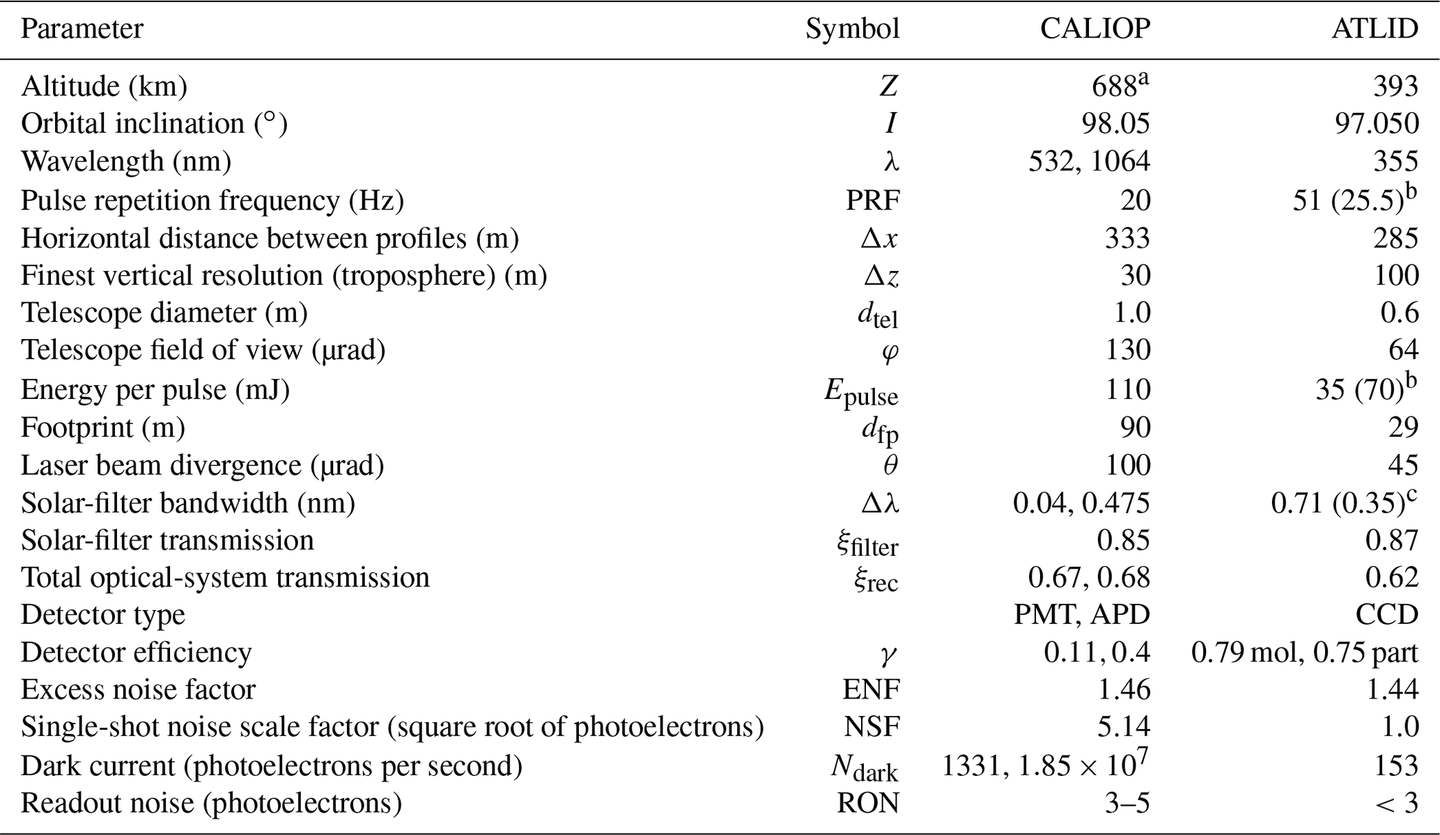
a The nominal orbit altitude at launch was 705 km but was lowered to 688 km in September 2018 to maintain formation flying with CloudSat. b The original pulse repetition frequency of ATLID laser is 51 Hz at the energy of 35 mJ per pulse, but the measurements will be doubled on board the satellite (do Carmo et al., 2021), so one can consider the effective frequency and energy per pulse to be equal to 25.5 and 70 mJ, respectively. c The solar-filter bandwidth of ATLID is 0.71 nm, but the transmission function of the Mie channel is approximately half of that, so one should calculate the solar noise in this channel with a narrower effective filter width.
When considering signal quality and performance, some parameters are in favor of CALIOP (telescope diameter, energy per pulse, solar-filter bandwidth), whereas others favor ATLID (altitude, noise level). In the next section, we show how these differences affect the detectability of clouds. We excluded the multiple scattering coefficient from the table since it is an important and complex parameter of lidar instrument which depends on its several parameters. Instead, we discuss it in a dedicated paragraph below.
2.2 Lidar equation
The formalism used in this work was described in Feofilov et al. (2022). In this section, we repeat only the basic definitions needed for understanding the material presented below. Since we will discuss both conventional (non-HSRL) and HSRL lidars, we will introduce necessary quantities in parallel and label them correspondingly: the molecular, particulate, and total components will get the indices “mol”, “part”, and “tot”, respectively.
An atmospheric lidar sends a brief pulse of laser radiation towards the atmosphere. The lidar optics collect the backscattered photons and drive them to a detector. The detected signal is time-resolved: supposing each photon traveled straight forward and back, each time bin corresponds to a fixed distance from the lidar to the atmospheric layer where backscattering occurred. The propagation of laser light through the atmosphere and backwards to the detector is described by the following lidar equation:
where ATB stands for attenuated total backscatter (m−1 sr−1), βmol(λ,z) and βpart(λ,z) are the wavelength-dependent molecular and particulate backscatter coefficients (m−1 sr−1), αmol(λ,z) and αpart(λ,z) are the extinction coefficients (m−1), Zsat is the altitude of the satellite, λ is the wavelength, and η is a multiple scattering coefficient (e.g., Platt, 1973; Garnier et al., 2015; Donovan, 2016).
For the HSRL lidar, one can write similar equations for the attenuated radiance backscattered from atmospheric particles and molecules (APBs and AMBs), respectively:
For cloud definition, we will also need to define the attenuated molecular backscatter for clear-sky conditions:
The physical meaning of η in Eqs. (1)–(3) is an increase in the number of photons remaining in the lidar receiver field of view (FOV) besides the ones directly backscattered by the layer, and its value depends on the type of scattering media, FOV of the telescope, and laser beam divergence. The typical value of η varies between 0.5 and 0.8 for commonly used lidars (Chiriaco et al., 2006; Chepfer et al., 2008, 2013; Garnier et al., 2015; Donovan, 2016; see also Appendix B of Reverdy et al., 2015). Setting η to 1 means no multiple scattering and would correspond to an infinitely narrow FOV telescope combined with an infinitely small laser beam divergence. In CALIOP cloud products up to version 3, the η was set to 0.6 for ice clouds, whereas for version 4.10 a temperature-dependent coefficient was used, which varied in between 0.46 and 0.78 (Young et al., 2018). For water clouds, the η values are derived from the relationship developed in Hu et al. (2006) (also see Table 4 in Young et al., 2018). A detailed modeling of η for different cloud types observed by CALIOP and ATLID (Shcherbakov et al., 2022) shows that η depends on the cloud thickness and type and that the ATLID values are somewhat higher than those of CALIOP. Based on these works, we set a fixed value of η to 0.6 for CALIOP and to 0.75 for ATLID. This is an approximation, and a more complex approach might be required for processing real data, but our tests show that the conclusions of the present work do not change if we vary η within ±0.1 either for CALIOP or for ATLID (but not for both).
2.3 Cloud detection and cloud variables
To characterize the scattering properties of the atmosphere, it would be convenient to use some ratio of attenuated backscatter values (Eqs. 1–4), which would have a clear physical interpretation. Due to attenuation of AMBs below the clouds, using it in the denominator is counterproductive, so the ATBmol(λ,z) is used instead, and the scattering ratio (SR) is defined as
Considering a single-pulse profile measurement, we define a layer as cloudy if the following two conditions are met:
The second condition in Eq. (6) comes from the fact that the molecular backscatter in the upper troposphere is weak and the fluctuation in ATB might cause a false cloud detection if only SR is used. With the second condition, the cloud detection is more robust. This definition is used in CALIPSO-GOCCP (e.g., Chepfer et al., 2008, 2010, 2013), and we suggest keeping it for other lidars to ensure consistency between cloud products as discussed later.
In application to ATLID, this will mean using the values recalculated to 532 nm of ATB, which will be estimated from Eq. (1): βpart(355 nm,z) and αpart(355 nm,z) retrieved from the measurements (Eqs. 2 and 3) and βmol(532 nm,z) and αmol(532 nm,z) retrieved or estimated from pressure-temperature profiles from reanalysis. In the numerical experiment below, we calculated ATB using the available pressure-temperature profiles and the formalism provided in Feofilov et al. (2022). Here, we reproduce Eq. (8) of this paper:
In this conversion, we assume that the spectral dependence of particulate backscatter (βpart(λ) and αpart(λ)) is weak at the wavelengths used in this study. In Beyerle et al. (2001) it is stated that this is generally true for cirrus. In Voudouri et al. (2020), the values at two wavelengths agree within (relatively large) error bars. Therefore, we do not attempt to compensate for the spectral dependence. The only area where we noticed that this approach does not work for real data is the polar stratospheric region, where a direct application of Eq. (7) leads to an overestimation of polar stratospheric clouds (PSCs) (Fig. 8b of Feofilov et al., 2022).
For the cloud properties, we use the same variables as in CALIPSO-GOCCP (Chepfer et al., 2010): cloud fraction CF(z), opaque cloud cover Copaque, and opaque cloud height Zopaque. If a given atmospheric layer was observed multiple times or if it was sampled vertically at several points, we define the cloud fraction profile CF(z) in a usual way:
where Ncld(z) is the number of times the conditions of Eq. (6) is met and Ntot(z) is the total number of measurements in this layer. The opaque cloud cover Copaque is used in long time series and is defined over the 2∘ × 2∘ latitude–longitude gridded data as follows:
where the first condition triggers the opaque cloud detection (Guzman et al., 2017), Nopaque_prof is the number of vertical profiles for which an attenuation corresponding to a presence of opaque cloud was found, and Ntotal_prof is the total number of measurements in a 2∘ × 2∘ grid box. For an individual lidar profile, Zopaque corresponds to an altitude of full attenuation of backscattered signal, whereas for gridded data, Zopaque is an opaque-cloud-cover-weighted sum (Guzman et al., 2017).
In this section, we search for useful cloud information regarding model evaluation that can be retrieved from the ATLID but cannot be obtained from the CALIPSO data. For this purpose, we use high-resolution cloud scenes (Sect. 3.1), simulate how they would be observed by ATLID and CALIPSO (Sect. 3.2), and compare the SR(z) profiles seen by the two lidars (Sect. 3.3) and the clouds detected by the two instruments (Sect. 3.4). To address the comparability of clouds observed by two spaceborne lidars, we used the existing methodology (Reverdy et al., 2015; Feofilov et al., 2022) but with a much finer-scaled cloud model, updated instrumental parameters of ATLID, and a new simulation chain which estimates noise at the detector level and propagates it to the cloud product level (the details are provided in Sect. 3.2.2 below). The main question we sought to answer in this section was whether ATLID can better observe optically thinner clouds than CALIPSO in daytime, a useful capability for evaluating thin cirrus clouds in climate models (e.g., Berry et al., 2019). At the same time, we checked whether the chosen cloud detection parameters and instrumental properties affect the detection of highly inhomogeneous low-level thick clouds.
3.1 Cloud-generating model
The 3DCLOUD model (Szczap et al., 2014) generates three-dimensional (3D) spatial structures of stratocumulus and fair-weather cumulus and cirrus that share some statistical properties observed in real clouds such as the inhomogeneity parameter ρ (standard deviation normalized by the mean of the water content) and the Fourier spectral slope close to between the smallest scale of the simulation to the outer scale Lout (where the spectrum becomes more flat). We assume that water content follows a gamma distribution. 3DCLOUD_V2 presented in Alkasem et al. (2017) is based on wavelet framework instead of the Fourier framework. First, 3DCLOUD assimilates meteorological profiles (humidity, pressure, temperature, and wind velocity) and solves drastically simplified basic atmospheric equations in order to simulate 3D water content. Second, the Fourier filtering method is used to constrain the intensity of mean water content, ρ, , and Lout, which are values provided by the user (Hogan and Illingworth, 2003; Kärcher et al., 2018).
Conditions of simulations to generate the stratocumulus in this study (see Fig. 1) are identical to those used in Szczap et al. (2014) for the DYCOMS2-RF01 case (the first research flight of the second Dynamics and Chemistry of Marine Stratocumulus) for the marine stratocumulus regime (Stevens et al., 2005). We have only changed the number of voxels in the x, y, and z directions to and Nz=50, respectively. The corresponding spatial resolutions were set to m and Δz=24 m, respectively. The vertical extension of the simulated area is still Lz=1200 m, but the horizontal extensions for this study are km.
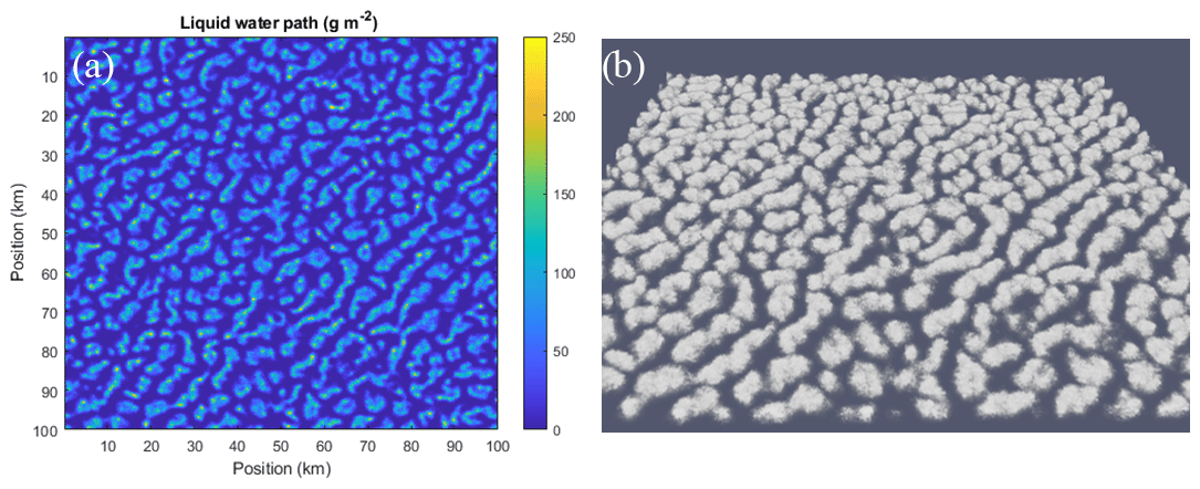
Figure 1Examples of the stratocumulus generated with 3DCLOUD: (a) 2D ice water path and (b) its volume rendering.
If the number of voxels is large, the 3DCLOUD and 3DCLOUD_V2 are very time-consuming (see Table 1 in Szczap et al., 2014) and cannot assimilate the fractional coverage for cirrus clouds. Therefore, we developed 3DCLOUD_V3 to overcome these two drawbacks for a cirrus cloud. This model will be published elsewhere. Here, we present only an outline of the 3DCLOUD_V3 algorithm.
To increase the calculation speed in 3DCLOUD_V3, we generate clouds using modified statistical tools developed as part of stage 2 of 3DCLOUD. The first stage of 3DCLOUD (i.e., the step of solving simplified basic atmospheric equations, which is very time-consuming) is no longer carried out in 3DCLOUD_V3. Thereby, 3DCLOUD_V3 can be seen as a purely stochastic cirrus cloud generator. The user has to provide, in addition to Nx, Ny, Nz, Δx, Δy, and Δz, the mean ice water path (IWP); Lout; the shape of the vertical profile of ice water content (IWC), ρ(z), and and of horizontal wind velocity components u(z) and v(z); and finally the cloud fraction CF. The shape of the vertical profile of IWC can also be stipulated (rectangular, upper triangle, lower triangle, and isosceles trapezoid; Feofilov et al., 2015). The algorithm works as follows:
-
The 3D isotropic field with a Gaussian probability density function (PDF) is generated from a 3D inverse Fourier transform assuming a random phase for each Fourier amplitude and a 3D spectral energy density with 1D spectral slope close to between the smallest scale of Lout.
-
The 2D Gaussian PDF is transformed into a 2D Gamma PDF at each z level, satisfying the values of IWC(z), ρ(z), and .
-
There is horizontal displacement, at each z level, of 2D IWC (to simulate fall streaks) computed from u(z) and v(z), based on the model of sedimentation proposed by Hogan and Kew (2005). In 3DCLOUD_V3, the user can choose the value of the sedimentation velocity: either constant or as a function of IWC (see formula in Fig. 12 in Heymsfield et al., 2017). Alternatively, the wind velocity vertical profile can be computed from a constant value of the vertical wind shear prescribed by the user; in this case, the user also has to provide the “generated-level height” as explained in Hogan and Kew (2005).
-
The vertical profile of the cloud cover is iteratively modified in order to obtain the CF value prescribed by the user.
Figure 2 demonstrates the examples of 2D IWP and the 3D IWC volume rendering of the cirrus generated with 3DCLOUD_V3, where , Nz=100, m, and Δz=20 m. The mean IWP is set to 1 g m−2. The IWC vertical profile shape is “rectangular”. The geometric depth is 2 km. The outer scale is Lout=20 km. We set the constant vertical wind shear to 5 m s−1 km−1 in the x and y directions, and the generated-level height is 400 m under the cloud top. The inhomogeneity parameter of IWC is ρ=0.4. The spectral slope β is equal to . Figure 2c shows the gamma-like PDF of the IWC (we ignored null values), and Fig. 2d shows the mean power spectra of IWP (and IWC) along x and y directions (and z direction), with the 1D spectral slope close to −2.0 (−1.3) between Lout=20 km and the finest spatial resolution. As expected, values of the spectral slope of IWP are smaller than those of IWC (i.e., the IWP signal is “smoother” than the IWC signal) because IWP is the vertically integral quantity of IWC. One can note that the IWC spectral slope is slightly smaller than the prescribed theoretical value because of the many null values of the IWC; we plan to remove this bias in the final version of 3DCLOUD_V3.
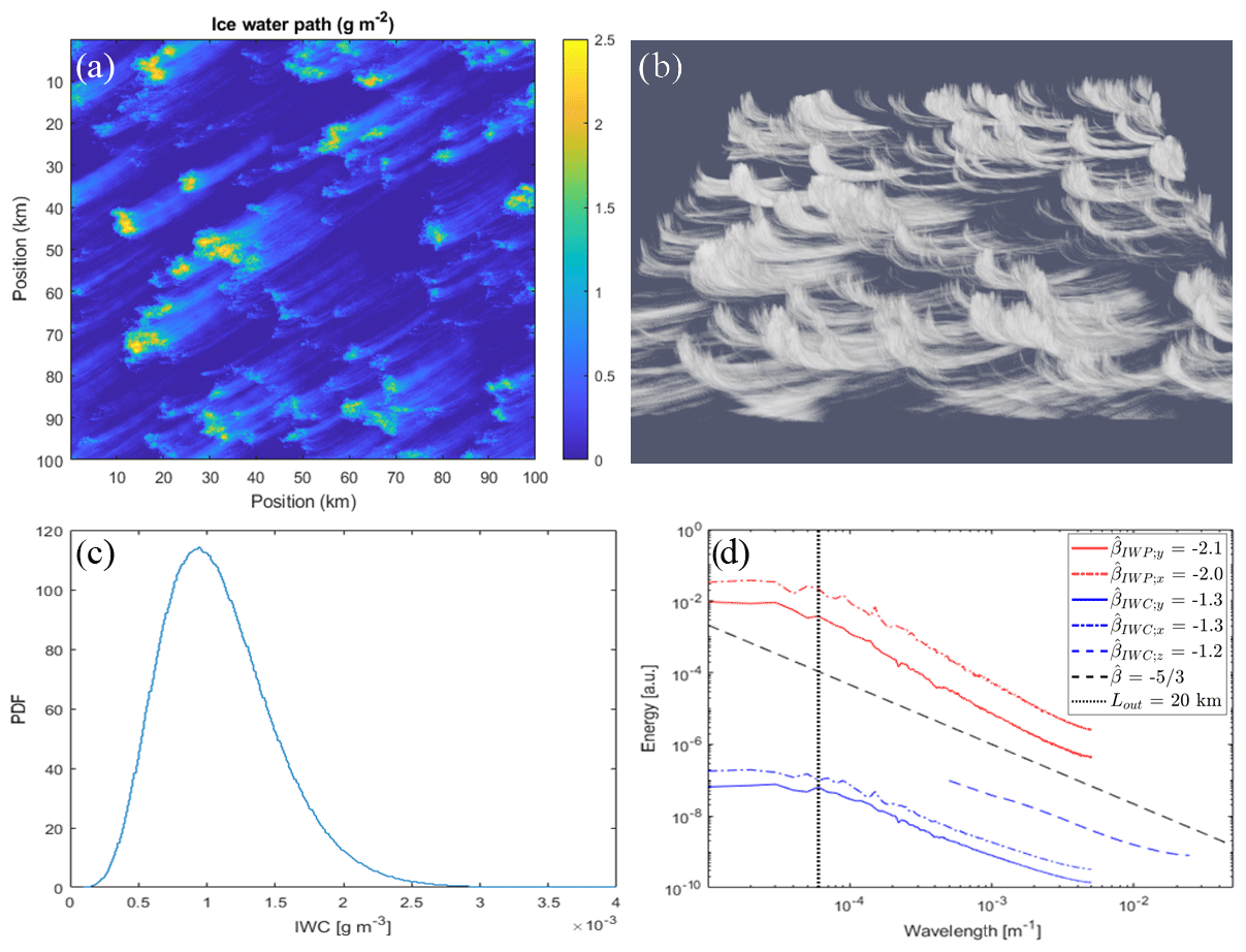
Figure 2Examples of cirrus generated with 3DCLOUD_V3: (a) ice water path and (b) its volume rendering; (c) IWC PDF; (d) mean 1D power spectrum of IWP (red curves) and of IWC (blue curve) following the x, y and z direction (solid, dash–dot and dashed line, respectively). A theoretical power spectrum with spectral slope is added (dashed black line). A dotted vertical black line indicates the outer scale Lout=20 km.
3.2 Numerical chain to simulate cloud observations by CALIOP and ATLID at high resolution
3.2.1 Creating pseudo orbits
We performed the following numerical experiment, outlined in the flowchart in Fig. 3. First, we created a gridded global atmosphere from the output of the U.S. Department of Energy's Energy Exascale Earth System Model (E3SM) atmosphere model version 1 (EAMv1; Rasch et al., 2019) for the conditions of autumn equinox in the Northern Hemisphere. Since we wanted to address both high- and low-level cloud detection, we picked up only the tropical part of the orbit between 5∘ S and 5∘ N and used this data as a set of smooth “background” profiles. Since this model does not provide the small-scale variability needed for our experiment, we used the subgrid model described in Sect. 3.1, which generates realistic cloud profiles at a grid comparable or finer than the distance between two consecutive footprints of studied lidars. To address the most challenging observation conditions, we picked up two cloud types: (1) thin cirrus clouds with optical depths (τ) of about 0.03–0.1 per layer (Sassen and Comstock, 2001) and (2) stratocumulus clouds with their high horizontal variability and large optical depths (up to 30 but with about one-third of semi-transparent clouds). These clouds were simulated using an updated 3DCLOUD_V3 model (see Sect. 3.3) and provided as gridded sets of ice water content (IWC) and liquid water content (LWC) values for cirrus and stratocumulus clouds, respectively. We do not consider another challenging case, a thin-cloud layer above a highly reflective cloud, but the daytime noise estimated for the stratocumulus scene will give an idea of what background noise will be interfering with the useful cloud signal in this case.
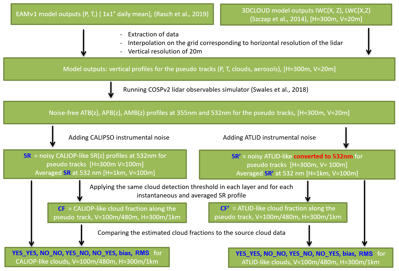
Figure 3Flowchart explaining the numerical experiment on comparing clouds retrieved from CALIOP and ATLID observations. Green boxes list the input and output data. Black text between boxes describes actions performed on each dataset. Blue text in the boxes marks the datasets used in the estimation. White text in square brackets in the boxes indicates horizontal (H) and vertical (V) resolutions of the datasets. Note that the ATLID SR′ values are estimated at 532 nm (see Sect. 2.3).
These gridded sets were converted to pseudo orbits by slicing them along the diagonal lines and arranging the slices into “lidar curtains”, each comprising 20 000 individual profiles and split into daytime and nighttime parts with 10 000 profiles each. This way we got almost seamless cloud distributions, which followed the variability prescribed by the 3DCLOUD_V3 model and at the same time resembled parts of real lidar orbits. We show the most representative parts of these pseudo orbits in Figs. 4 and 5 for cirrus and stratocumulus clouds, respectively, and we discuss them below.
With these two datasets covering both the daytime and the nighttime scenes, we performed a full series of simulations, explained in Fig. 3. Namely, we fed the high-resolution atmospheric inputs described above to the CALIOP and ATLID simulators (Chepfer et al., 2008; Reverdy et al., 2015) included in the Cloud Feedback Model Intercomparison Project Observational Simulator Package version 2 (COSP2) simulator (Swales et al., 2018). These simulators do not account for instrumental noise effects, so their outputs were processed by a third part of the simulation chain (Fig. 3), which estimates noise and its propagation in the lidar system.
3.2.2 Estimating lidar signals and noise
As mentioned above, the outputs of COSP2 simulator are the noise-free APB (355 nm,z) and AMB (355 nm,z) profiles for ATLID and noise-free ATB (532 nm,z) profiles for CALIOP, both calculated at a horizontal resolution of 300 m and vertical resolution of 20 m. To estimate the noise for these profiles and to propagate it further to SR (532 nm,z) for CALIOP and to recalculated SR for ATLID, we calculated the signals from scratch using the corresponding instrumental parameters introducing measurement noise as follows.
We start with a laser emission and estimate the number of emitted photons per sounding pulse, measured at the output of the sounding unit:
where Epulse is the energy per laser pulse, h is Planck's constant, c is the speed of light, λ is the wavelength, and ς is an effective coefficient of optical throughput of the emission path of the lidar. In the present work, it is assumed that there is no optical loss in the emission path and ς is equal to 1. The numerical solution of the Eqs. (1)–(3) yields the number of photons per range gate (titi+Δti), which we will denote as ti, coming through the CALIOP receiver or through the ATLID receiver before splitting into molecular and particulate components in the HSRL module (compare to Eqs. 2 and 3):
where are the photons backscattered by molecules and particles, respectively; Ω(zi) is an altitude-dependent solid angle with zi corresponding to the time of flight ti between the satellite and the measured layer i; and ξrec is the receiver's transmission.
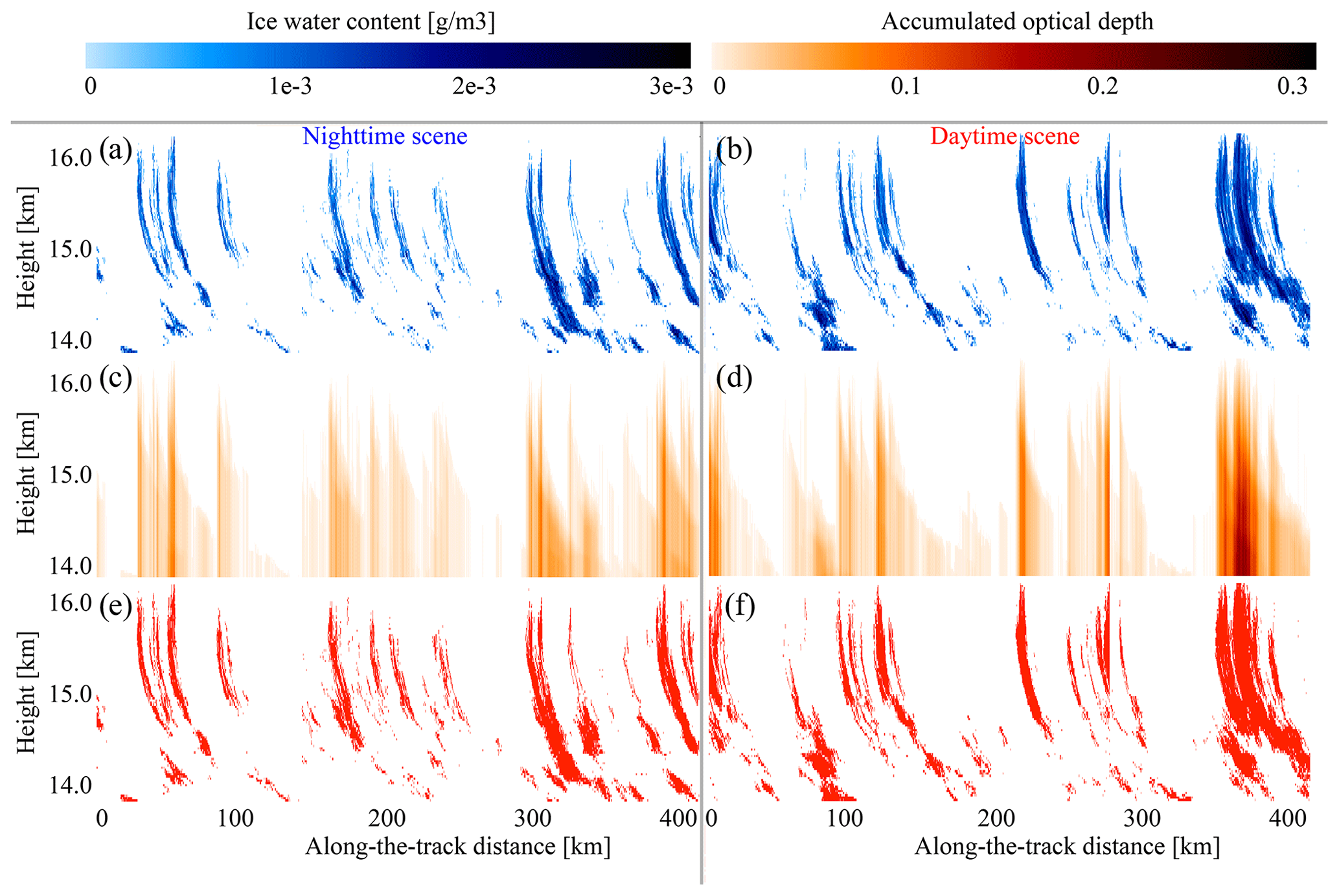
Figure 4Example of cirrus cloud input data from the 3DCLOUD model used in the simulation: (a) ice water content (IWC), with night corresponding to one piece of the orbit; (b) IWC, with day corresponding to another piece of the orbit; (c) accumulated optical depth starting from the cloud top at night; (d) same as (c) during the day; (e) cloud mask at night; and (f) cloud mask during the day. We set the cloud mask to 1 whenever IWC > 0. The cloud masks presented here are called the “reference dataset” in the rest of the paper.
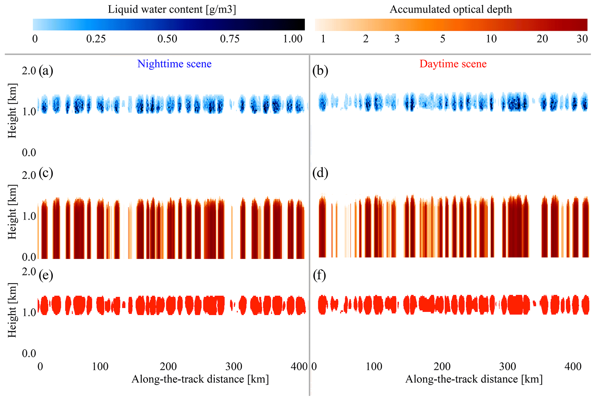
Figure 5Same as Fig. 4 but for stratocumulus cloud scenes. Note the color scale difference between Figs. 4 and 5.
For an HSRL lidar, the molecular and particulate components are supposed to be registered individually, but this separation is not ideal because of the crosstalk between the channels: a part of molecular backscatter comes at the same wavelength as the original laser radiance and it “contaminates” the particulate channel, which is centered at this wavelength. Overall, the HSRL system is characterized by four crosstalk coefficients, Cmm, Cpp, Cmp, and Cpm. The first two show a contribution of the molecular and particulate channels to themselves, and in the ideal HSRL they should be equal to 1. The second pair shows how much energy “leaks” from a molecular channel to a particulate one and vice versa. In an ideal HSRL, these coefficients would be equal to 0. In the operational retrieval, these coefficients will be determined through a continuous calibration procedure performed on the orbit. For this exercise, we estimated these coefficients from the Fabry–Pérot interferometer spectral curves (Cheng et al., 2013): Cmm=0.815, Cpp=0.60, Cmp=0.185, and Cpm=0.40. In the case of a non-ideal HSRL, the number of photoelectrons produced by each detector per range gate is as follows:
where γ and ξrec are the detector's quantum efficiency and transmittance of the optical path, respectively. To come back to “pure” and used in the retrieval, one has to solve this system:
Besides the components related to atmospheric backscatter properties, the and are affected by “parasite” solar backscattered photons during the daytime, which are not correlated with the laser shots. To estimate the solar background add-on to and , one has to solve the radiative transfer equation for the radiation emitted by the Sun, backscattered by air and particles in the atmosphere and by the surface in the direction of the spaceborne lidar, and attenuated by the atmospheric layers:
where is the top-of-atmosphere solar flux at wavelength λ and for filter width Δλ; and represent the proportion of the incoming solar radiance reflected in the direction of lidar; ϕm(SZA), ϕp(SZA), and ϕsurf(SZA) are the scatter plots for the angle between the Sun and the nadir view of lidar for molecular scattering, scattering on particles, and scattering from the surface, respectively; zsat is the altitude of a satellite; and Asurf is the surface albedo. We assumed Lambertian scattering from the surface with albedo equal to 0.08 for ocean and 0.15 for land (arbitrary values), we used Rayleigh scattering phase function for the molecular component, and we used the geometric-optics phase function approximation for particulate scattering.
The solar photons pass through the optical system and HSRL, hit the detectors, and produce the “solar-noise photoelectrons”:
where and represent the convolution of the solar-filter spectral curve with the interferometric spectral curve for a given channel (see the comment on solar-filter bandwidth in Table 1). In addition to solar noise, there is always a dark current of the detector (Ndark) and readout noise (RON) which are added to the signal. Since the and , Ndark, and RON are registered along with and during daytime, they enter Eqs. (15) and (16) and affect the retrieval. For the non-HSRL lidar:
where γ and ξrec stand for the corresponding parameters of non-HSRL lidar and represents the transmission coefficient of a solar rejection filter, which is equal to a ratio of an integral of the spectral transmission curve of the filter to a full spectral width of the filter. A quick back-of-the-envelope estimate of the ratio of solar photons coming to the particulate detector of ATLID to the number of solar photons reaching the surface of CALIOP's detector per same sampling interval is
So, at first sight, the ATLID retrieval should be less solar-contaminated than CALIOP. But, this ratio alone is not enough for such a conclusion because the solar photons should be compared to the useful signal. Below, we show the results of simulations for two atmospheric scenarios which consider two-way radiative transfer both for solar radiance and for lidar sounding radiance and add the noise of the remaining detection path.
Now, when all the components of the signal are known, we can estimate the daytime and nighttime signal and noise and propagate them to the retrieved parameters. It is important to mention that the instruments compared in this work use the detectors of different types. Namely, the CALIOP lidar uses a photomultiplier tube (PMT), whereas the ATLID lidar detects the backscatter with the help of a charge-coupled device (CCD). Besides different characteristics like gain or dark current (see Table 1), these detectors are not the same in terms of applicable noise statistics (Liu et al., 2006). Even though the incoming photon flux distributions for both instruments are Poisson, the photoelectrons produced by the PMT do not follow a strict Poisson distribution. It is known that for Poisson-distributed signals, a one-to-one relationship exists between the mean and the variance of the photocurrent. As Liu et al. (2006) show, the mean and the variance of the PMT photocurrent are also proportional but not one to one, and the corresponding noise scale factor (NSF) has to be applied to estimate random errors for lidar systems using PMTs or avalanche detectors. The NSF is linked to an excess noise factor (ENF), but it is not equal to it. For the PMTs with identical gain factors m for each dynode, the ENF is given by (Kingston, 1978; Liu and Sugimoto, 2002)
For the analog detection, the NSF in the multiplied photoelectron domain can be either calculated from the detector's ENF and gain or estimated from the solar-noise-dominated signals (Liu et al., 2006):
where σ(Ndet), var(Ndet), and 〈Ndet〉 are the standard deviation, variance, and mean of the signal, respectively. The NSF value provided in the CALIPSO L1 version 4.10 files is equal to 5.14. However, using this value in synthetic-noise calculations leads to an overestimation of the daytime noise, so for the calculations below we took a more conservative value of NSF =3.16. One can write the expressions for the variances of CALIOP and ATLID signals in the analog detection domain through the number of photoelectrons calculated for each channel:
We draw the reader's attention to the fact that the detector's parameters in Eq. (31) are not equal to those in Eqs. (29) and (30) and that for real calculations one has to use the values from Table 1 or a similar source. The variances of molecular, particulate, and total incoming photon fluxes, which are finally used in the optical property retrievals, are estimated in accordance with the standard error propagation formulae applied to the equations above:
where the represents the covariance of molecular and particulate channels. This term is required because the signals in the channels are coupled through non-zero crosstalk.
When the variances are known, the original noise-free AMB, APB, and ATB profiles are modified by random noise, which is modulated by the standard deviation calculated from the variances, and the results are saved. If horizontal or vertical signal averaging is involved, the noise is scaled inversely proportional to a square root of the number of samples within the averaging interval.
3.2.3 Useful lidar signals and their SNRs
To address the information content of the backscattered radiance, it makes sense to define a useful signal and to estimate the SNR for this signal. For CALIOP the useful signal is represented by ATB(λ,z) (see Eq. 1), whereas ATLID can measure the molecular and particulate backscattered radiances separately, so it would be logical to call the APB(λ,z) (see Eq. 2) a signal which carries the information about the cloud and look at its SNR. For the sake of simplicity, we do not discuss here the perpendicular channels of these two space lidars assuming that the backscattered depolarized radiance is detected the same way, and adding the processing of this component to the formalism above would not change the conclusions of this work. Another aspect that we do not discuss here is the change in cloud microphysics, which can also affect the cloud detection and cloud radiative effects. We consider and model only the cloud occurrence, cloud cover, and cloud detectability.
For the simulated CALIOP signals, we estimate SR(z) at 532 nm and CF(z) according to Eqs. (6) and (7). The simulated ATLID signals are converted to equivalent 532 nm SR′(z) (see Sect. 2.2 and Feofilov et al., 2022). Then we calculate CF(z) for ATLID using Eqs. (6) and (7) with the same thresholds, and then we analyze the resulting cloud fraction.
To quantify the lidar cloud detection agreement and disagreement regarding the reference cloud dataset, we distinguish four cases: (1) when the lidar detects the actually cloudy layer as cloudy (YES_YES case); (2) when there is no cloud and the lidar does not detect a cloud (NO_NO); (3) when the lidar does not detect an existing cloudy layer (YES_NO or false negative); and (4) when the lidar detects a cloud, whereas the layer does not contain a cloud (NO_YES or false positive). We will define their occurrence ratios as
The sum of all four ratios in Eq. (35) yields unity. A perfect match between the cloud distribution in the atmosphere and the product retrieved from the measurement would be when RYES_YES(z)+ RNO_NO(z)=1 and .
3.3 Simulated ATLID and CALIPSO lidar profiles over cirrus and stratocumulus scenes
The most representative parts of pseudo orbits generated with the help of the 3D_CLOUDV3 model (Sect. 3.3) are shown in Figs. 4 and 5 for cirrus and stratocumulus clouds, respectively. We arbitrarily split the “cloud curtain” generated from the output of this model (Sect. 3.2) to “daytime” and “nighttime” by setting the solar zenith angle (SZA) to 45 and 120∘, respectively. These values are not linked with the cloud formation mechanisms in the 3D_CLOUDV3 model; they are just needed for a second half of the simulator chain (see noise-related boxes in Fig. 3). In Fig. 4a and b, one can see a fine structure of modeled cirrus clouds. Looking at Fig. 4c and d, one can say that the clouds are optically thin. This combination makes the detection of the clouds marked in Fig. 4e and f challenging.
The stratocumulus clouds shown in Fig. 5 belong to another category of challenging observations. The clouds are closely spaced along the horizontal axis, and at the same time they are optically thick: about two-thirds of the clouds have optical thickness larger than 3 (Fig. 5c, d), but the scene also contains about one-third of semi-transparent clouds like the ones that were reported in Leahy et al. (2022). From Fig. 5c and d, one can conclude that at present there is no space-based measurement that can retrieve all the optical properties of cloud layers shown in Fig. 5e and f. Another problem of these clouds is that their horizontal averaging might bias the estimated cloud fraction (see, e.g., Fig. 4 and discussion of Feofilov et al., 2022).
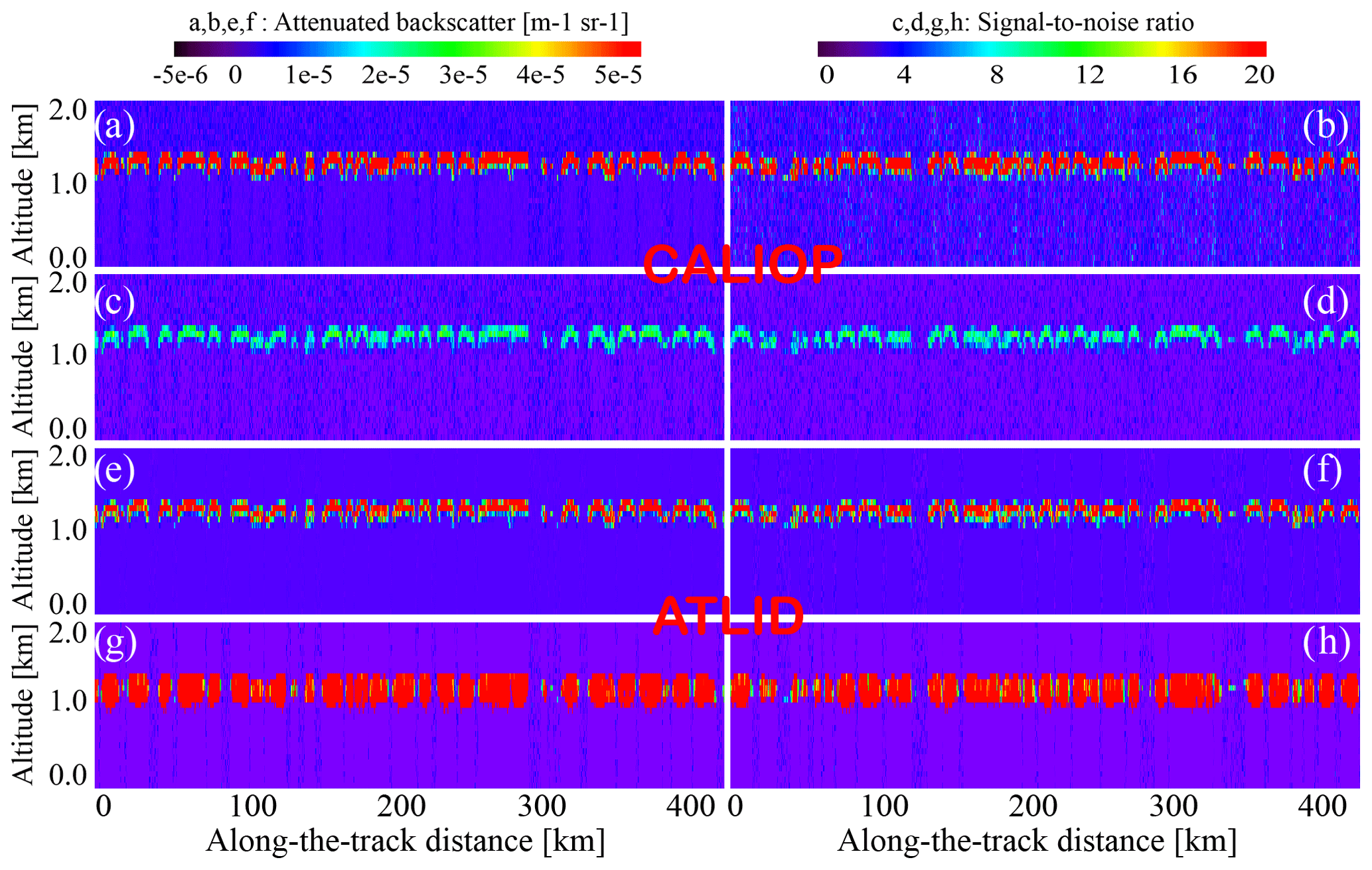
In Figs. 6 and 7, we demonstrate the differences between two lidars for four scenes (cirrus/stratocumulus clouds, day/night) using the simulated backscatter signal. For the cirrus cloud scene (Fig. 6), both the ATB(532 nm,z) of CALIOP and the APB(355 nm,z) of ATLID show a detectable signal in the areas marked by a cloud mask in Fig. 6e and f. But if one defines the signal detection level as 3σ, one will see that a part of thin clouds will be missing. This is not surprising since we compare a “pure” modeled cloud with its noisy representation in the measuring system. What can be estimated from the image is the potential reliability of cloud detection from ATLID and CALIOP: according to the SNR values (Fig. 6g, h vs. c, d), the APB(355 nm,z) signal from ATLID (Fig. 6e, f) reaches higher SNR values than the ATB(532 nm,z) signal from CALIOP (Fig. 6a, b). This hints at the fact that the cloud detection from this instrument might be somewhat better than that from CALIOP and that one can lower the detection threshold and still get the cloud instead of noise. This is a subject of one of the experiments described below. As for the daytime vs. nighttime difference, we do not see a big change between the left-hand side and right-hand side panels for ATLID (Fig. 6e–h), whereas the CALIOP shows higher noise in Fig. 6b and d. We note here that the calculations were performed for the cases when only a thin cirrus cloud was present in the atmospheric column, whereas the rest of it corresponded to clear-sky conditions. In the real world, though, the second cloud layer beneath cirrus might increase the solar noise (see the right-hand side panels of Fig. 7), and this will adversely affect the thin-cloud detection, especially from the CALIOP measurements. This is explained by a larger field of view of the CALIOP lidar (see Table 1). In our exercise, we wanted to estimate the best achievable results for a given cloud scene for each instrument and to compare the lidar performances. This way, the conclusions made below for the daytime scenes refer to the minimal differences between the two instruments. As for the stratocumulus clouds (Fig. 7), both the signals and SNRs are strong for both lidars, day and night. The altitudes beneath these clouds correspond to areas without a useful signal: at these heights, the signal is already attenuated by a cloud above, and the attenuation is so strong that even the cloud base is not visible at optical wavelengths (e.g., Guzman et al., 2017). Another remarkable feature shown in this plot is higher daytime noise for CALIOP (Fig. 7b, d). Even though this high noise level does not affect the stratocumulus cloud detection itself, it might affect the aforementioned higher-level cloud detection, and, from this point of view, ATLID has an advantage over CALIOP.
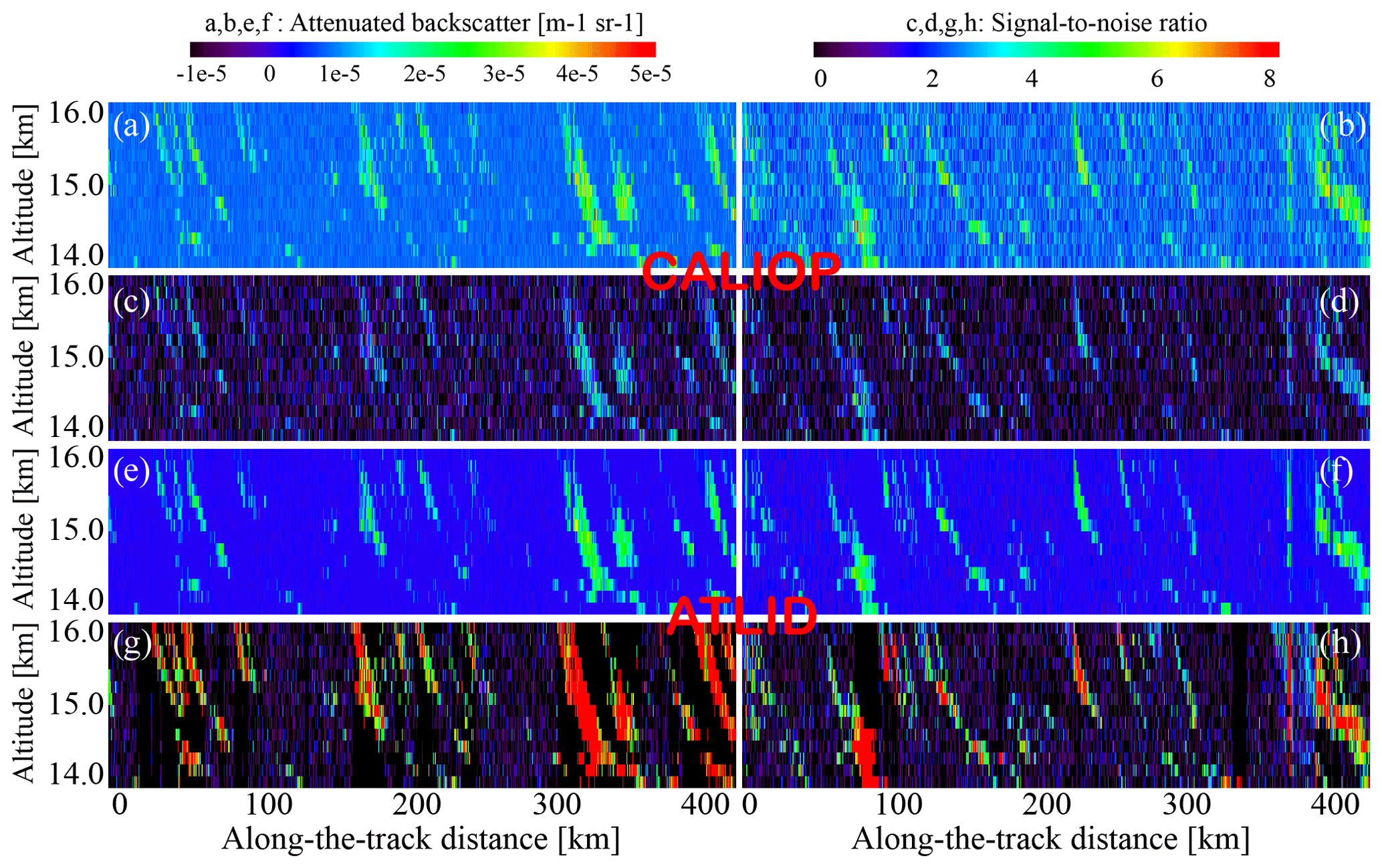
Figure 6Signals and signal-to-noise ratio for the cirrus cloud scene. CALIOP: (a) ATB (532 nm, z) at night for one piece of the orbit, (b) ATB (532 nm, z) during the day for another piece of the pseudo orbit, (c) SNR at night, and (d) SNR during the day. ATLID: (e) APBs (355 nm, z) at night, (f) APBs (355 nm, z) during the day, (g) SNR at night, and (h) SNR during the day. Note that the scene contains only these clouds and a clear sky below. For the reflective clouds beneath the cirrus layer, the daytime noise will be higher (see the right-hand side panels of Fig. 7).
Summarizing, one can say that the ATB(532 nm,z) signals of CALIOP and the APB(355 nm,z) signals of ATLID carry similar type information for the same cloud scenes, but their SNRs suggest (a) that the daytime cloud detection from ATLID should be more reliable and (b) that one can lower the detection threshold for this instrument without admixing numerous noise-triggered clouds. Let us now see how the signal quality transforms into the product quality and, in particular, to cloud detection quality.
3.4 Capability of ATLID to better detect optically thinner clouds than CALIPSO
Here, we describe the test we performed seeking to answer whether the cloud detection limits (Eq. 6) defined in Chepfer et al. (2010) could be lowered to detect thinner clouds. For this test, we followed the second half of the flowchart (Fig. 3) and calculated the SR(532 nm,z) for CALIOP and the CALIOP-like SR(532 nm,z) for ATLID (Eqs. 2–3), but we changed the cloud detection thresholds of Eq. (6) to the following ones:
Then we estimated the cloud fractions and statistical agreement with the source cloud data (Eqs. 6, 7). The threshold in the left-hand side of Eq. (36) implies that the particulate backscatter in a layer, which we call a cloudy one, is twice the molecular one.
The threshold in the right-hand side of Eq. (36) corresponds to the absolute values of ATB(532 nm,z) recalculated for at the height of 8 km (Chepfer et al., 2010), but overall the rationale for selecting these very values is based on the SNR values levels we observed in the test simulations. Further lowering the threshold will lead to an increased number of false-positive cloud detections in ATLID.
Since the “native” CALIOP profiles are averaged over three points above 8 km, we applied an averaging procedure over ∼1 km distance to all simulated signals and repeated the analysis. To compare apples to apples in terms of signal statistics, we averaged over four CALIPSO shots and over two effective ATLID shots, yielding the actual average over 1330 and 1140 m, respectively. To reduce the number of plots, we do not show the instantaneous profiles without the averaging, but in Table 2 we provide the estimates for them (seek columns marked with “Averaged” with N).
In Fig. 8a and b, the SR(532 nm,z) has the same patterns as the ATB(532 nm,z) signals in Fig. 6a and b. But the daytime noise is more pronounced in this presentation, partially because of the chosen color scale. However, not all the noise from Fig. 8b propagates to Fig. 8d. This is because of a second condition of Eq. (36): the variations are partially filtered out by imposing a condition on the ATB(532 nm,z) signals with respect to ATBmol(532 nm,z). Still, the daytime scene contains a lot of false detections marked by red in Fig. 8d. The overall characteristics of CALIOP cloud detection for this scene estimated over the whole simulated cloud dataset can be found in the second and sixth columns of Table 2. The bottom two lines of this table refer to the detectability of a cloud in the whole layer: if some values of the SR(532 nm,z) triggered cloud detection, we calculated the cloud fraction similar to Eq. (7) and then compared the resulting series of cloud fractions with the reference one defined from the source dataset. The “total score” line refers to the cloud detection statistics and is defined in the caption. As one can see, the strong daytime noise of CALIOP prevents the correct cloud detection, mostly due to large number of false-positive cloud detections (NO_YES). The bias and the RMS (root mean square) rows show the biggest change when passing from nighttime to daytime conditions.
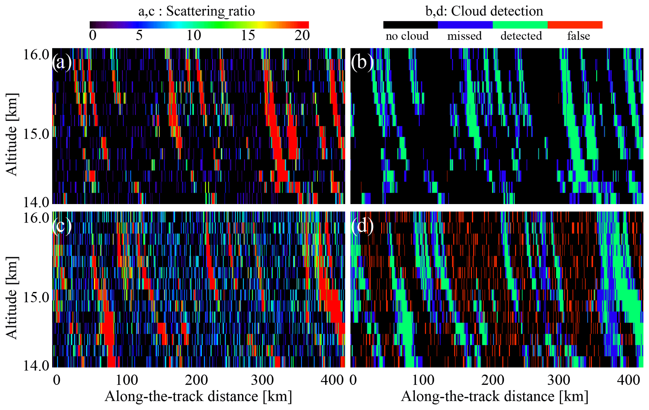
Figure 8Scattering ratio and cloud detection estimated for cirrus clouds observed by CALIOP using Eq. (36): (a) scattering ratio at night, (b) cloud detection at night, (c) scattering ratio during the day, and (d) cloud detection during the day. Note the color scale difference for (a) and (c) compared to (b) and (d).
The same analysis performed for ATLID (Fig. 9) shows less daytime noise (compare Fig. 9b to Fig. 8b), and the cloud detection quality for the clouds defined using Eq. (36) is better than that of the CALIOP (compare Fig. 9d to Fig. 8d). The corresponding columns of Table 2 tell us that for ATLID the number of false detections during day and night is approximately the same, whereas for CALIOP using the Eq. (36) for the detection dramatically increases the number of false detections during daytime. We should also stress here that the obtained result is a lower estimate because we used the scenes without underlying clouds, which could reflect more solar radiance and further contaminate the observations. For these scenes, the difference between ATLID and CALIOP will be even larger.
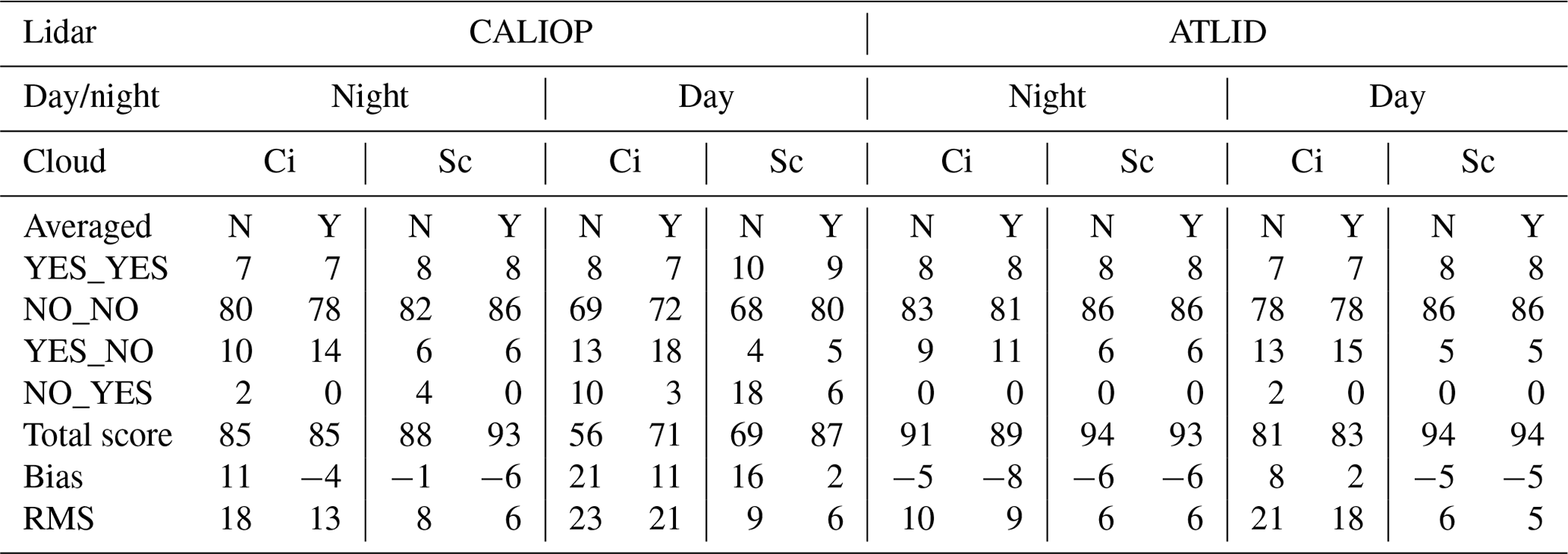
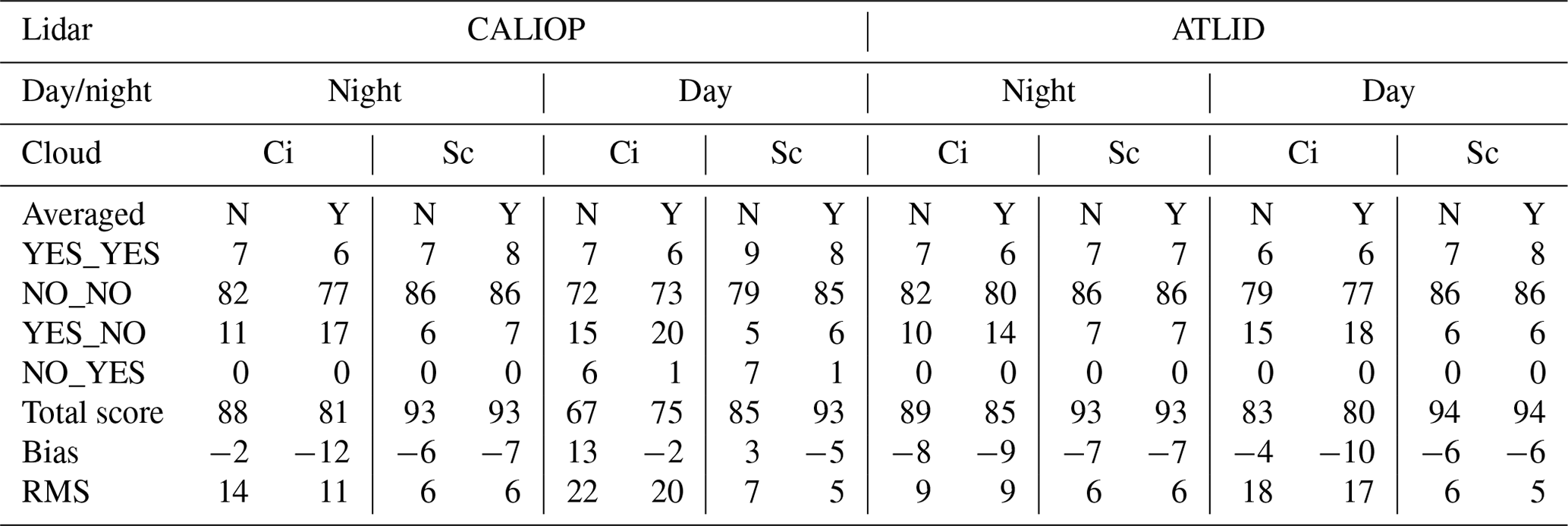
Table 2Cloud detection statistics for CALIOP and ATLID when the cloud definition corresponds to and (Eq. 36). The bias and RMS values are defined for the clouds detected in the columns (see text), and we define the total score in percent as . Ci: cirrus clouds, Sc: stratocumulus clouds.
The same type plots built for the stratocumulus clouds (Figs. A1 and A2 in the Appendix A for CALIOP and ATLID, respectively) show a different picture. Strong signals and large SNRs shown in Fig. 5 help to unambiguously identify the cloud. The large fraction of underestimated clouds shown in blue in Figs. A1cd and A2cd corresponds to cloud parts below the opaque cloud top layer, which are not accessible for the instruments observing the scene from above. As with cirrus clouds, the false-detection rate is higher for CALIOP during daytime.
For CALIOP, the 1 km averages reduce the number of false detections and improve the total score for daytime simulations for cirrus. For ATLID with its lower daytime noise, the averaging procedure does not change the cloud detection quality that much. For the stratocumulus clouds, the averaging procedure is not required for ATLID since sometimes it can lead to overestimating the cloud fraction (e.g., Chepfer et al., 2008; Feofilov et al., 2022). For CALIOP, it improves the score because of suppression of sporadic noise-induced “clouds” above the real cloud layer (Fig. A1d).
Overall, the ATLID-related columns in Table 2 demonstrate more consistency between daytime and nighttime cloud amounts and reference data than the CALIOP-related ones, and ATLID daytime cloud quality is better than that of CALIOP, whereas the nighttime results are comparable. Our tests show that if the CALIOP-like solar filter were used in ATLID, one could lower the thresholds of Eq. (36) down to and without losing the quality of cloud retrievals, whereas the same thresholds applied to CALIOP would give completely unacceptable results for daytime conditions.
Of course, the examples considered in this section do not cover the whole range of high-, middle-, and low-level clouds, but they draw a line between the threshold values that can be used for cloud definition for CALIOP and ATLID and show that the difference is linked to noise characteristics of the instruments. This result suggests that ATLID should be able to better observe optically thinner clouds than CALIOP in daytime at full horizontal resolution.
To illustrate this point, we used the available dataset for cirrus and estimated the minimal detectable backscatter (MDB) for ATLID in terms of equivalent ATB(532 nm,z) for comparison with CALIOP values obtained for 5 km horizontal averaging of cirrus measured at 15 km height (McGill et al., 2007). For this numerical experiment, we used noisy APBs and noise-free AMBs to keep the consistency with our approach of cloud detection using only one noisy component, the particulate one. For this horizontal averaging, we obtained MDB = 3.0 ± 1.0 × 10⁻⁷ m−1 sr−1 for the nighttime and MDB = 4.0 ± 1.0 × 10⁻⁷ m−1 sr−1 for the daytime in equivalent ATB(532 nm) values, whereas for CALIOP we obtained MDB = 4.0 ± 2.0 × 10⁻⁷ m−1 sr−1 for the nighttime and MDB = 1.3 ± 0.2 × 10⁻⁶ m−1 sr−1 for the daytime in its native ATB(532 nm). The daytime value estimated for CALIOP is in good agreement with the measured one (McGill et al., 2007), whereas the estimated nighttime value is somewhat lower than the measured MDB = 8.0 ± 1.0 × 10⁻⁷ m−1 sr−1. From this comparison, we cannot conclude that the ATLID will provide better sensitivity to thin clouds during nighttime, but we can conclude that its daytime thin-cloud detection at 5 km averaging capacity should be comparable to that of CALIOP for the nighttime, and this will be an important achievement for daytime vs. nighttime cloud comparison. Using the cloud detection thresholds defined by Eq. (36) and refined for the real data flow using the methodology outlined above, the CLIMP short-term product will be produced.
4.1 Capability of CLIMP and CALIPSO-GOCCP to detect the same clouds
One of the overarching goals of our study is to develop a method for merging the data from several spaceborne lidars into a continuous cloud record to detect long-term changes and get a seamless cloud climatology. Since the low threshold tested in the previous section revealed the sensitivity mismatch between the two instruments, we had to test whether the cloud detection thresholds developed for CALIOP (Chepfer et al., 2010) are applicable to ATLID and whether the clouds retrieved using these thresholds are consistent between the two lidars. For this exercise, we followed the same scheme as in the previous section, but this time the clouds were defined in Eq. (6) as in Chepfer et al. (2010) and the follow-up works (e.g., Cesana et al., 2019; Guzman et al., 2017).
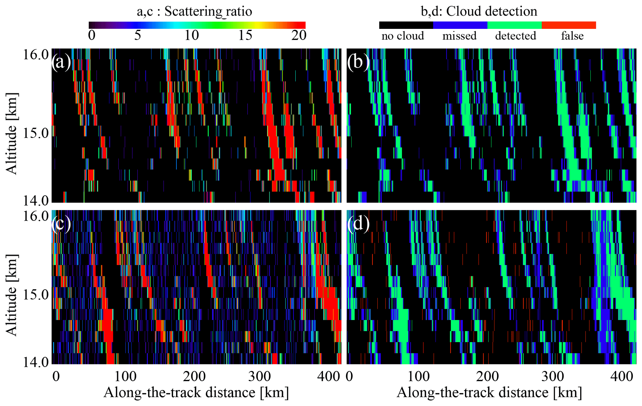
Figure 10 demonstrates the daytime and nighttime scattering ratios above the detection thresholds (Eq. 6) and the corresponding cirrus cloud detection statistics for CALIOP. The SR(532 nm,z) in Fig. 10a and b demonstrates the same patterns as the ATB(532 nm,z) signals in Fig. 6a and b. As expected, this time the daytime noise is less pronounced (compare Fig. 10b to Fig. 8b). Still, the daytime scene contains a certain number of false detections marked in red in Fig. 10d. The same analysis performed for ATLID (Fig. 11) also shows somewhat less noise in daytime (compare Fig. 11b to Fig. 9b). The cloud detection quality of ATLID is like that of CALIOP (see Table 3). In this setup, the ATLID is just slightly better than CALIOP with its somewhat higher rate of false detections during the day (compare panels c and d of Figs. 8, 9, 10, and 11 and the corresponding columns in Table 3). For stratocumulus clouds (Figs. 1 and 5), with their strong signals, the agreement between CALIOP and ATLID is also better than for the clouds defined by Eq. (36) (compare panels c and d of Figs. A1, A2, A3, and A4). The 1 km averaging further improves the agreement between the datasets (Table 3).
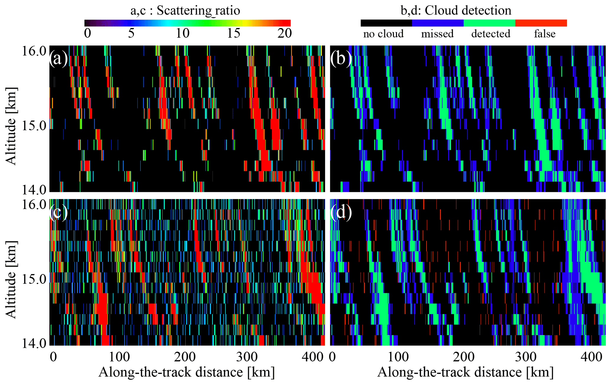
Figure 10Scattering ratio and cloud detection statistics estimated for cirrus clouds observed by CALIOP using Eq. (6): (a) scattering ratio at night, (b) cloud detection at night, (c) scattering ratio during the day, and (d) cloud detection during the day. Note the color scale difference for (a) and (c) compared to (b) and (d).
Summarizing, using the thresholds (Eq. 6) to define the clouds makes the cloud datasets from CALIOP and ATLID comparable. Further adjustment will be needed for real ATLID data to compensate the effects of the diurnal cycle (Noel et al., 2018; Chepfer et al., 2019; Feofilov and Stubenrauch, 2019). Other compensations might be required when the real ATLID data become available. Since there is a high chance that there will be no overlapping period for these two satellite instruments, an intercalibration procedure will be required. For this, one can use the average cloud amount for low, middle, and high clouds in different zones (tropics, middle latitudes, and polar) to track the changes and to introduce feedback to the cloud detection algorithm. This way, the number of cases measured for each zone will be high, and the uncertainty will be low. The daytime and nighttime observations should be considered separately to address the diurnal cycle and daytime noise issues. In the sections below, we assume that the intercalibration has been performed and that the cloud datasets agree.
Table 3Cloud detection statistics for CALIOP and ATLID in the case when the cloud is defined as and (Eq. 6).
4.2 Numerical chain to simulate long-term lidar record and method to quantify time of emergence
The previous section shows that ATLID and CALIOP data may be merged to build a long-term dataset, even though their instrumental or orbital differences might necessitate further reconciliation. Here we suppose perfect reconciliation will eventually be reached, and we build a long-term space lidar synthetic dataset spanning more than 30 years to examine when a change in cloud properties attributable to human-induced warming would be detectable in the lidar cloud record according to climate model simulations. This approach is directly inspired by the one pioneered in Chepfer et al. (2018) and later expanded in Perpina et al. (2021).
We use climate predictions from IPSL-CM6 (Institut Pierre Simon Laplace climate model; Boucher et al., 2020) and CESM2 (Community Earth System Model; Hurrell et al., 2013), two ocean–atmosphere coupled GCMs which took part in Climate Model Intercomparison Project (CMIP) Phase 6 (Eyring et al., 2016). We use predictions that start in 2008 and end in 2034 and follow the RCP8.5 (Representative Concentration Pathway) scenario, which tracks the observed CO2 emissions closely (Schwalm et al., 2020). Predictions are provided as monthly grids with spatial resolutions of 1.27∘ × 2.5∘ on 79 vertical levels (IPSL-CM6) and 1.25∘ × 0.94∘ on 40 vertical levels (CESM). On these predictions of atmospheric conditions, we apply the COSP1.4 lidar simulator (Sect. 3.2), which generates on similar spatial grids the monthly averaged cloud properties that would be observed by a spaceborne lidar flying over the simulated atmosphere. In addition to the simulation steps described in Sect. 3.2, here, as a first step of the simulation, for each grid box of the GCM-created atmosphere an ensemble of subgrid-scale profiles are stochastically generated by the Subgrid Cloud Overlap Profile Sampler (Klein and Jakob, 1999). Each of these profiles is fed to the COSP simulator, which generates a synthetic lidar profile, on which cloud detection is performed. All subgrid-scale cloud detection profiles are eventually averaged to generate a single vertical profile for each grid box (see Chepfer et al., 2008, for details).
From the synthetic cloud properties, we considered two climate diagnostics whose trend should be related to climate change: first the fraction of opaque clouds Copaque, defined as the number of lidar profiles in which an opaque cloud is detected in a given latitude–longitude grid box divided by the total number of profiles sampled in the same grid box. Opaque clouds are responsible for the majority of cloud radiative effects in the tropics (Vaillant de Guélis et al., 2017), and the cloud amount has been identified as one of the main drivers of cloud feedbacks on climate (Zelinka et al., 2016); thus the fraction of opaque clouds should be closely tied to climate change. Second, we considered the altitude of full attenuation Zopaque (Guzman et al., 2017) averaged over all opaque profiles in every grid box. The vertical distribution of clouds is closely linked to their longwave radiative impact and to climate change (Vaillant de Guelis et al., 2018), and their altitude is expected to increase by several hundred meters per century (Richardson et al., 2022). Altitude is among the cloud properties whose change is expected to be detectable the earliest using active remote sensing (Chepfer et al., 2014; Takahashi et al., 2019; Aerenson et al., 2022).
From the GCM predictions, the COSP lidar simulator generates monthly grids of Copaque and Zopaque that we spatially average over the tropics (30∘ S–30∘ N) to get monthly time series. We deseasonalize those time series to get their monthly anomalies over the 2008–2034 period. For any time t along these time series, the record length is equivalent to the period between 1 January 2008 and t, and we computed the trend w(t) as the linear regression of the time series of anomalies over that period. The uncertainty σw(t) in the trend w(t) at time t was computed, as in Chepfer et al. (2018), as , with n being the number of years in the record at time t, φ being the lag−1 autocorrelation coefficient of the series between 0 and t, and σN being the standard deviation of the noise remaining in the series between 0 and t once it has been deseasonalized and the autocorrelated part has been removed.
The following analysis focuses on the tropical regions (30∘ S–30∘ N), where the atmospheric circulation will be impacted by the weakening of the Hadley and Walker circulations expected in the upcoming century by most climate predictions (Davis and Rosenlof, 2012; Su et al., 2014; Kjellsson, 2015; Chemke, 2021). These changes will have important effects on the spatial distribution of tropical clouds (Su et al., 2014), which provide the basis for our climate diagnostics. Cloud opacity is one of the cloud properties most closely linked to their radiative impact (Zelinka et al., 2012), which explains why our diagnostics are based on the properties of opaque clouds (as in Perpina et al., 2021). The results below assume it will be possible to process ATLID measurements in such a way that CLIMP and GOCCP cloud properties are consistent.
4.3 How many years of ATLID observation are required in addition to CALIPSO to evaluate the climate model prediction of cloud changes?
Figure 12 shows how the uncertainty in the retrieved trend for Copaque changes with the length of the record of lidar-based cloud properties, starting in 2008, according to predictions from IPSL-CM6 (blue) and CESM1 (orange). The uncertainty is generally the largest and fluctuates most when the record is short and decreases and stabilizes as the record gets longer. At any time t if we require a 95 % confidence level in the prediction and assume trends are normally distributed, the real trend will lie in the w(t)±2σw(t) interval. The sign of the trend will be robust once . This is when the uncertainty in the trend becomes small compared to the trend itself and marks the time of emergence of cloud change induced by anthropogenic warming. This occurs earlier for strong, stable trends and might never occur for very small trends or trends whose sign changes over time. Times of emergence in the Copaque time series are indicated in Fig. 12 with triangles for three confidence levels (50 %, 70 %, and 95 %). Reaching a reliable sign requires a longer record if the required confidence level is strong.
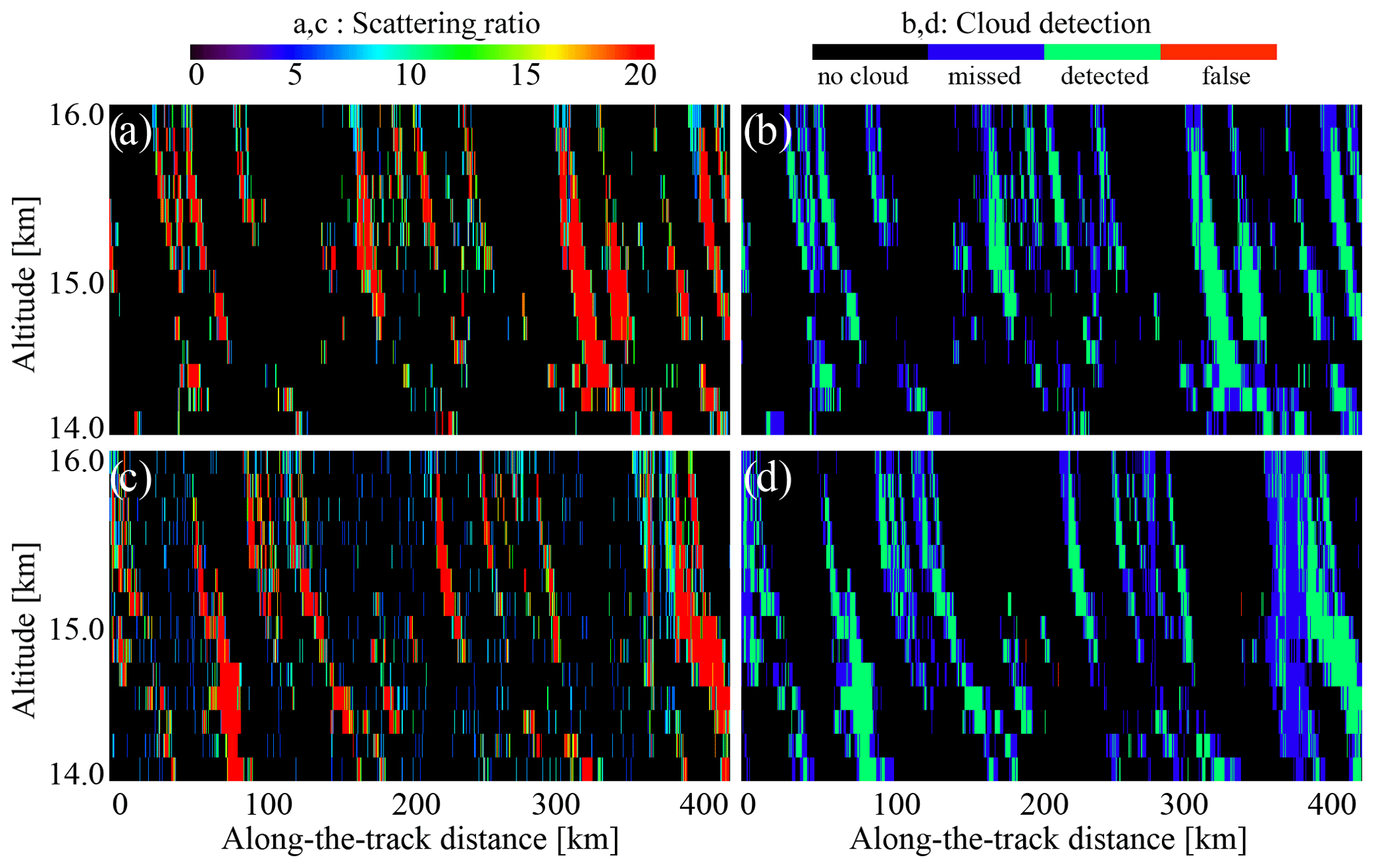
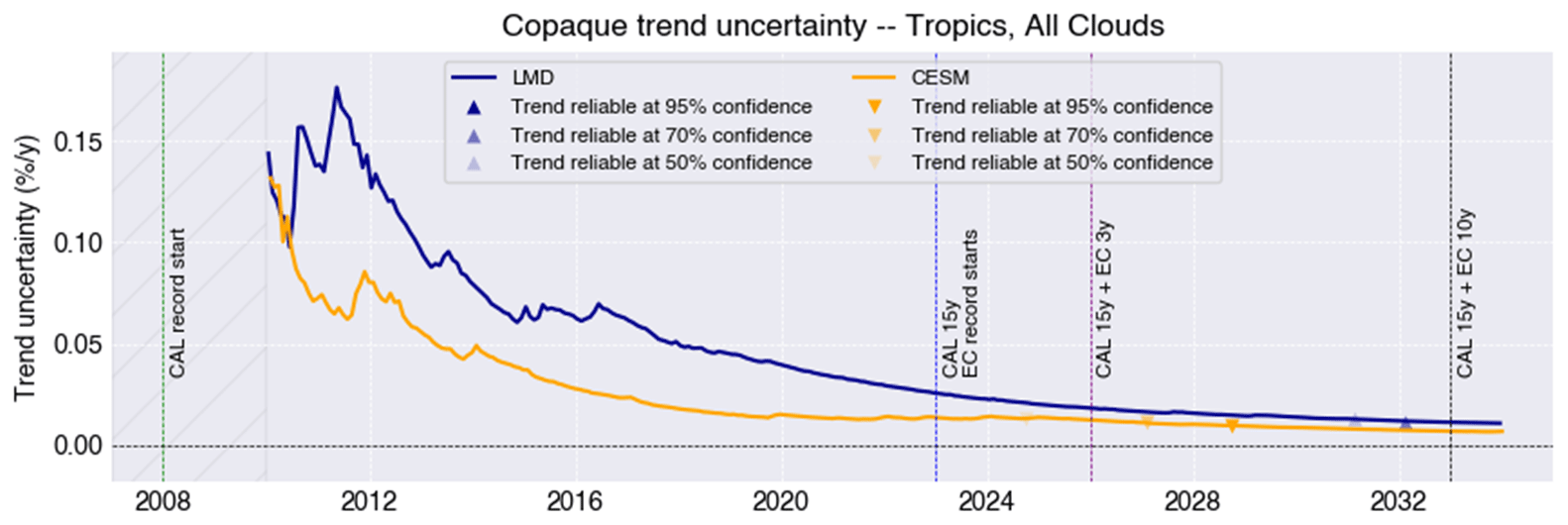
Figure 12Evolution of the uncertainty in the Copaque trend as a function of the length of the spaceborne lidar record, according to atmospheric conditions predicted by IPSL-CM6 (blue; Laboratoire de Météorologie Dynamique, LMD) and CESM (orange) in the period between 2008 and 2034 following the RCP8.5 scenario. The first 2 years of the record (2008–2010) are considered in the analysis, but trend uncertainties during that period are very large and are masked in the figure to improve the legibility of later years. CALIPSO's (CAL) planned end of operation (2023) is marked by a vertical blue line. Supposing EarthCARE (EC) begins operation right afterward, its nominal 3-year operation point is marked by a vertical purple line, and an optimistic 10-year operation point is marked by a vertical black line.
According to predictions from IPSL-CM6 (blue), a reliable trend should emerge from the natural variability at a 50 % to 70 % confidence level between 2030 and 2032. In other words, IPSL-CM6 predicts that revealing a reliable long-term trend in the fraction of opaque clouds would require an uninterrupted spaceborne lidar record of 22 years, which would be achievable if EarthCARE operates for at least 7 years. Reaching 95 % confidence levels on the retrieved trend would require extending the record beyond 25 years, most probably through another spaceborne lidar mission further in time. CESM1, meanwhile, predicts that a reliable long-term trend in the fraction of opaque clouds (at similar confidence levels between 50 % and 70 %) would be reached between 2025 and 2027, requiring 2 to 4 years of EarthCARE operation. A highly reliable trend (95 % confidence levels) would be detectable in 2029, after 6 years of EarthCARE operation. In summary, if a 50 % confidence level is acceptable, detecting a reliable trend would either be possible within the EarthCARE nominal operation time frame (2 years after launch), according to CESM1, or require EarthCARE to operate 4 years beyond its planned lifetime, according to IPSL-CM6.
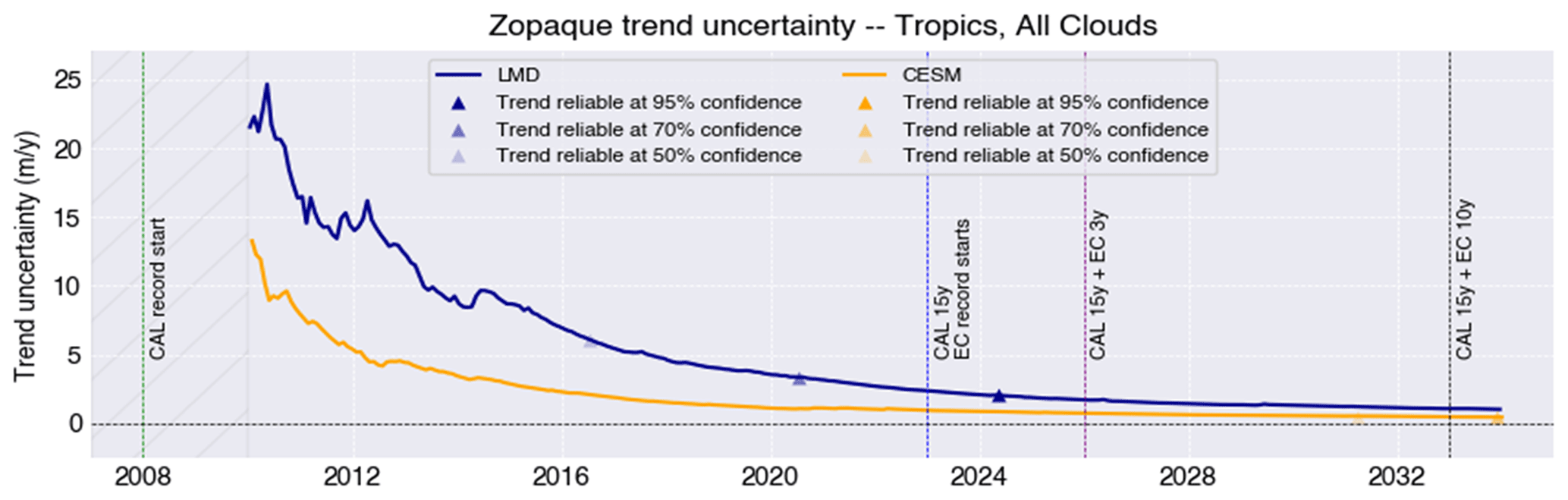
If we consider the Zopaque diagnostic (Fig. 13), the IPSL-CM6 model now predicts a trend will be detectable at high 95 % confidence levels in 2024, i.e., 1 year into EarthCARE's nominal operation period. Meanwhile, according to CESM1 predictions, detecting a reliable trend (even at a modest 50 % confidence level) would require EarthCARE operating for 8 years, 5 years beyond its nominal operation time frame. This very fast detection of a reliable Zopaque trend predicted by IPSL-CM6 is consistent with how this model expects important and fast changes in the vertical distribution of opaque clouds in the tropics (Perpina et al., 2021).
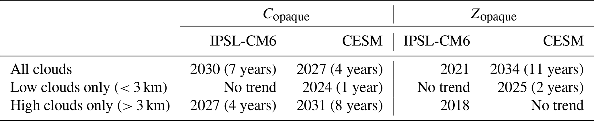
We sum these results up in Table 4, which in addition provides similar record lengths to detect reliable trends when considering grid boxes dominated by either low or high clouds. Tropical low opaque clouds include sparse shallow cumulus (Konsta et al., 2012) and optically thicker stratocumulus along the western coasts of continents (Guzman et al., 2017), both confined to the boundary layer and most frequent in subsidence regions. By contrast, tropical high opaque clouds are more localized and strongly correlated with deep convection. Since both kinds of clouds are driven by very different processes, it is not unreasonable to assume they will probably evolve differently in the upcoming century, which justifies their separate studies. In practice, we identified grid boxes dominated by low clouds as those where Zopaque was below 3 km and high-cloud grid boxes as those where Zopaque was above 3 km. The results, shown in Table 4, suggest that the nominal ATLID (EarthCARE) operation will be enough to validate or invalidate the trends in opaque tropical low clouds predicted by CESM. It will be possible to validate or invalidate other model-based cloud predictions only if EarthCARE performs beyond its nominal lifetime (which is not impossible, as CALIPSO demonstrated) or if measurements from a follow-up spaceborne lidar mission after ATLID are included in the cloud profile record. These results are consistent with the trends, uncertainties, and times of emergence found when conducting a relatively simpler comparison of HadGEM2-A (Hadley Centre Global Environment Model) predictions in current vs. +4 K conditions (Chepfer et al., 2018). Needless to say that the treatment of any follow-up mission (e.g., Atmosphere Observing System, AOS; Aeolus-2) will require the compensation for all the differences between the lidars like it is done in this work.
Table 4When will a spaceborne lidar record starting in 2008 be long enough to enable a reliable detection (at 70 % confidence level) of Copaque or Zopaque trends according to predictions from IPSL-CM6 or CESM? The required years of EarthCARE operation are shown in parentheses, supposing they begin in 2023. The monthly evolution of the trend uncertainties for low and high clouds are provided in Figs. B1 and B2 of Appendix B.
As stated up front, these results depend on rather strong hypotheses of perfect continuity and perfect intercalibration between the consecutive spaceborne lidars that provide the measurements from which the cloud properties are derived. Imperfect continuity would occur if, for instance, EarthCARE starts operation later than CALIOP stops. The missing years in the record would delay the detection of a reliable trend by at least the same time period (Chepfer et al., 2018). Perfect intercalibration supposes the effects of instrumental differences in technical specifications (wavelengths, pulse energy, field of view, etc.) and orbital characteristics (local time of overpass, altitude) on lidar measurements are reconciled somehow. For instance, ATLID operates at 355 nm and CALIOP operates at 532 nm, and the impact this has on measurements can be reconciled by converting the ATLID signal at 532 nm as done in the current study, but the costs of this conversion are not completely understood and will require re-examination when actual ATLID data are available. Imperfect intercalibration could lead to offsets in one spaceborne lidar's record compared to the other and would increase the uncertainties in the retrieved trends. Increased delays between the operation of both instruments would complicate their intercalibration. The different local times of overpass (01:30 and 13:30 local solar time, LST, for CALIPSO; 06:00 and 18:00 LST for EarthCARE) are also quite problematic, since each instrument will sample clouds at a different phase of their diurnal cycle (Noel et al., 2018; Chepfer et al., 2019; Feofilov and Stubenrauch, 2019). In particular, this will impact high clouds related to deep convection that exhibit a marked diurnal cycle. It is out of the scope of the present work to evaluate how this change could bias the retrieved long-term trends. The same applies to a follow-up lidar mission, which may or may not operate at the same orbit with the same local solar time of overpass and may or may not measure the depolarized backscatter.
Finally, the times of emergence presented here must not be understood as definite but as predictions by climate models. It is worth noting, for instance, that, according to predictions from IPSL-CM6, a reliable trend should already be readily detectable in the existing record of Zopaque that is today only built on CALIOP (CALIPSO) (Table 4). Such a trend has not been identified yet. This is consistent with the fact that in current climate conditions IPSL-CM6 overestimates the altitude of opaque clouds in tropical convective regions and brings them significantly higher (+ 2 km) near the end of 21st century (Perpina et al., 2021). Such rapid changes are not present in CESM predictions. These important model differences highlight the crucial need for continued long-term cloud lidar observations able to monitor the actual cloud changes and disambiguate model predictions.
This study presents the physical basis for the ATLID cloud climate product named CLIMP. This product builds on previous work on CALIPSO, a space lidar dedicated to cloud and aerosol observations like ATLID. CALIPSO data have been used for 16 years to evaluate the description of clouds in climate models using a dedicated product named GOCCP and a dedicated lidar simulator named COSP lidar. The present work also builds on recent work on AEOLUS, a space lidar with HSRL capability operating in the UV, like ATLID. Based on this legacy, we have defined the CLIMP-ST (Short-Term) and CLIMP-LT (Long-Term) products, both dedicated to cloud climate studies. Both contain the same variables as GOCCP (see Table D1 in Appendix D) on the same horizontal and vertical resolutions, but CLIMP-ST and CLIMP-LT have different cloud detection thresholds because they aim to tackle slightly different science objectives.
The CLIMP-ST product is designed to make full use of the ATLID capability for evaluating cloud description in climate models. CLIMP-ST is expected to contain optically thin cloud detected in daytime conditions at full resolution that were not observed by former space lidars at such high spatial resolutions during daytime. This new information, if confirmed in actual data, will help make progress regarding our current understanding of processes tied to thin ice clouds in the climate system. It will help evaluate the description in climate models of optically thin clouds in regions where they are frequent and important for climate, for example in the tropics and polar regions.
The CLIMP-LT product is designed to detect the same clouds as CALIPSO-GOCCP. Merging CLIMP-LT with GOCCP will allow for building a multi-decadal cloud profile record, useful to monitor the cloud inter-annual natural variability and cloud changes induced by human-caused climate warming. This record, if quality is sufficient, will be useful for evaluating climate prediction of cloud changes and for helping reduce uncertainties in model-based climate feedbacks and climate sensitivity.
To design CLIMP-ST and CLIMP-LT, we examined the differences between CALIOP and ATLID, space lidars that operate at different wavelengths and use different observation techniques and detectors. We sought to answer two questions. (1) Can the HSRL capability of ATLID help reconcile its cloud retrievals with the CALIOP record? (2) Does the cloud product retrieved from ATLID observations compare well with the one retrieved from CALIOP observations, and if so, how many years of ATLID observations are needed to detect trends in opaque cloud cover or altitude of opaque clouds, assuming ATLID operation will follow CALIOP without a gap?
To answer these questions, we coupled the outputs of the 3DCLOUD model with the COSP2 simulator and added instrumental noise for two cloud scenes, thin cirrus clouds at ∼ 15 km in the tropics and stratocumulus clouds at ∼ 1 km height. CALIOP and ATLID orbits over these cloud scenes were simulated both for nighttime and daytime conditions, at full vertical and horizontal ( km) resolution and at 1 km horizontal resolution. Then, we applied a wavelength conversion algorithm to ATLID observations to convert UV lidar profiles into 532 nm lidar profiles and added synthetic noise generated for each instrument in accordance with its characteristics.
We addressed the first question for CLIMP-ST. We showed that the lower daytime noise of ATLID allows for applying more sensitive thresholds for cloud detection ; ATB(532 nm,z) than for CALIPSO at full spatial resolution in daytime without introducing a bias. This suggests that ATLID may provide new information on optically thin clouds at daytime conditions at full spatial resolution.
We addressed the second question for CLIMP-LT. We search for consistency between ATLID and CALIPSO-GOCCP in cloud detection; therefore we applied the same cloud detection threshold ; ATB(532 nm,z) to both instruments, then their nighttime cloud products are comparable, whereas the daytime CALIOP clouds are characterized by a somewhat higher false-detection rate. This suggests ATLID and CALIPSO might observe the same clouds, with some adjustment in the cloud detection scheme. Then we analyzed 24 years of predictions from two general circulation models (IPSL-CM6 and CESM2) in the RCP8.5 scenario, coupled with the COSP lidar simulator. We show that IPSL-CM6 predicts the opaque-cloud-cover trend detection will require 7 years of ATLID operation besides the existing CALIOP cloud dataset, whereas CESM2 predicts the opaque-cloud-cover trend can be detected in 4 years. For the clouds above 3 km altitude, these numbers change to 4 and 8 years, respectively, and for the altitudes below 3 km the IPSL-CM6 clouds indicate no trend and CESM cloud trend detection will require 1 year of ATLID operation. These differences in climate predictions highlight the need for a multi-decadal cloud lidar record.
The current results rely on a comparison of exactly the same atmospheric scenes “virtually observed” by two space lidars, and they were obtained in the framework of comparing the cloud detection capabilities of these two instruments. However, the comparison of the actual ATLID measurements with actual CALIOP ones will face with an uncompensated difference linked to the sampling of local solar time by CALIOP and ATLID. The difference in the diurnal cycle will bias the detected cloud amount and height. This is a separate issue that should be compensated for, and this should be a subject of a separate work. Moreover, the comparison of actual ATLID measurements with CALIOP ones will probably face unexpected differences other than the ones foreseen in this paper. Therefore, the CLIMP algorithm will require an adjustment after ATLID launch to take those into account.
That being said, this study suggests that it is likely that ATLID will provide new information useful to help evaluate cloud description in climate models beyond the existing space lidar observations. Moreover, merging the ATLID data with the CALIOP data will probably provide important information on cloud response to climate warming.
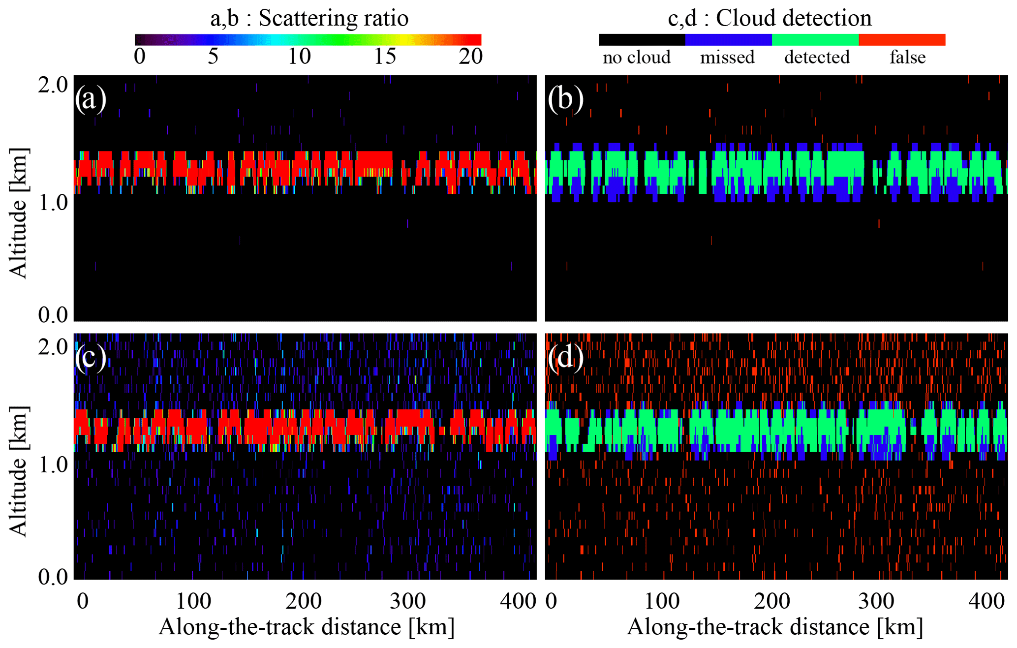
Figure A1Scattering ratio and cloud detection statistics estimated for stratocumulus clouds observed by CALIOP using Eq. (36): (a) scattering ratio at night, (b) cloud detection at night, (c) scattering ratio during the day, and (d) cloud detection during the day.
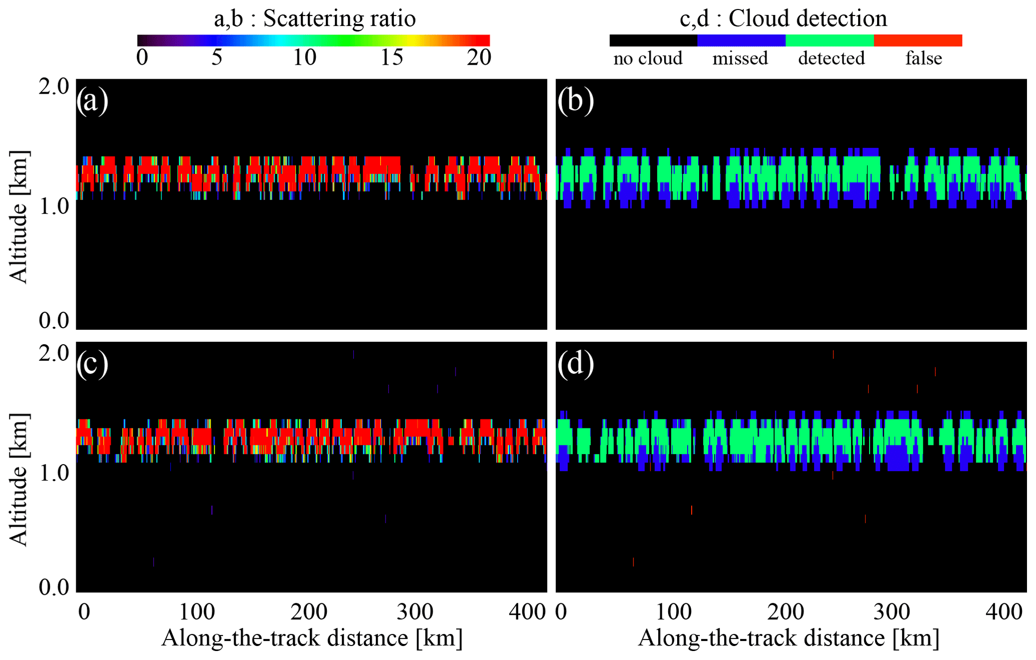
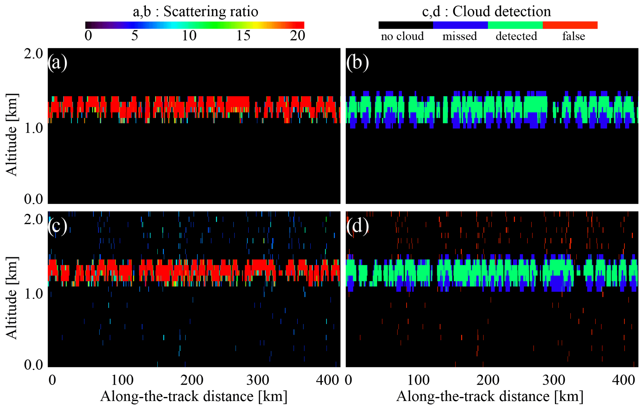
Figure A3Scattering ratio and cloud detection statistics estimated for stratocumulus clouds observed by CALIOP using Eq. (6): (a) scattering ratio at night, (b) cloud detection at night, (c) scattering ratio during the day, and (d) cloud detection during the day.
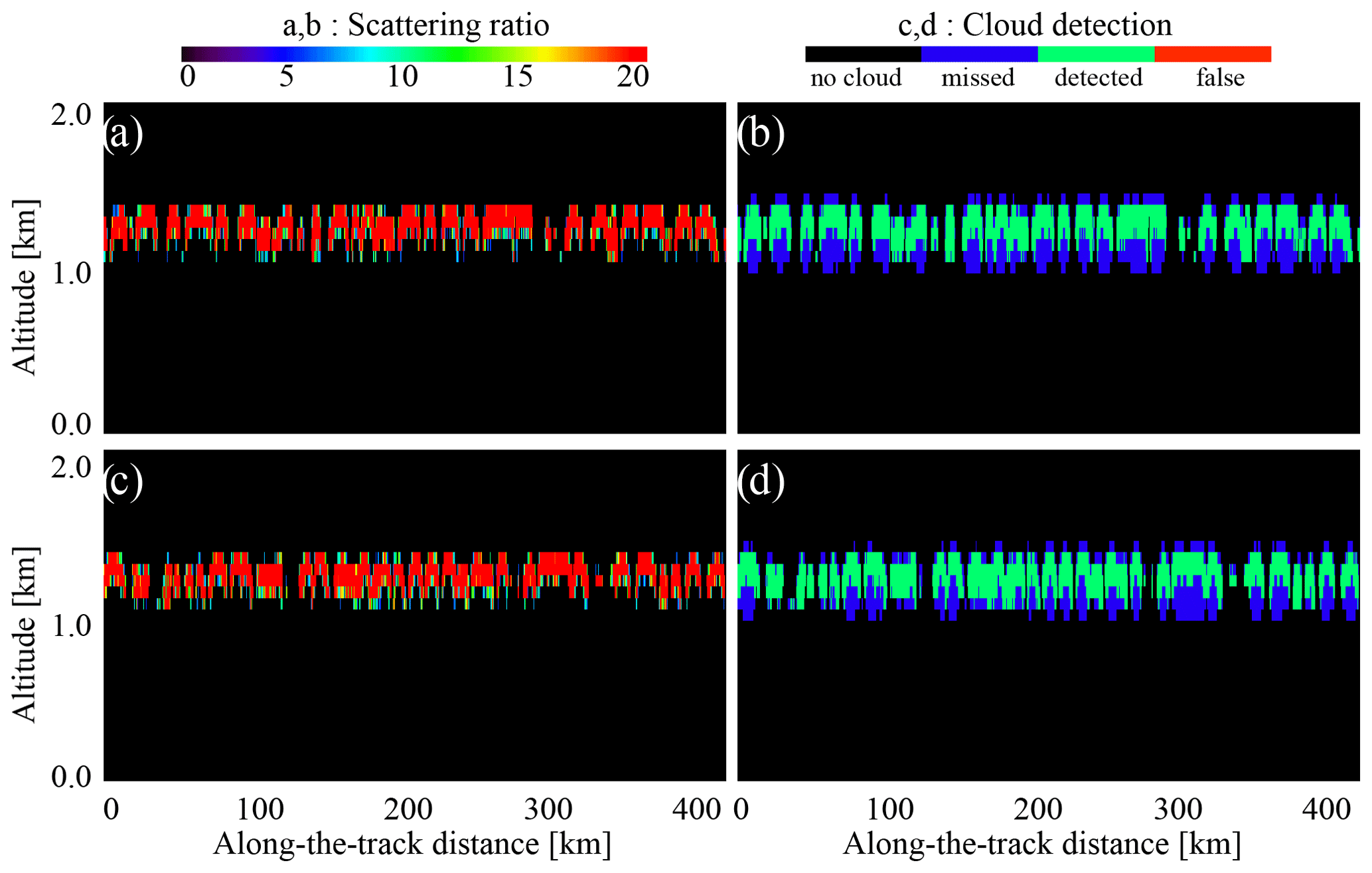
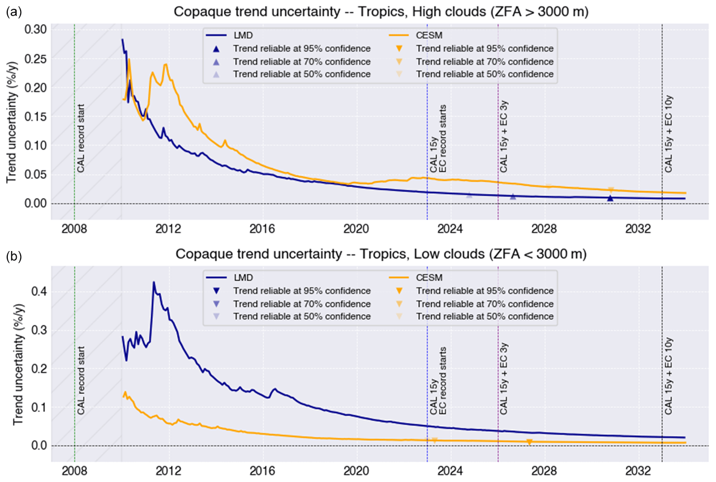
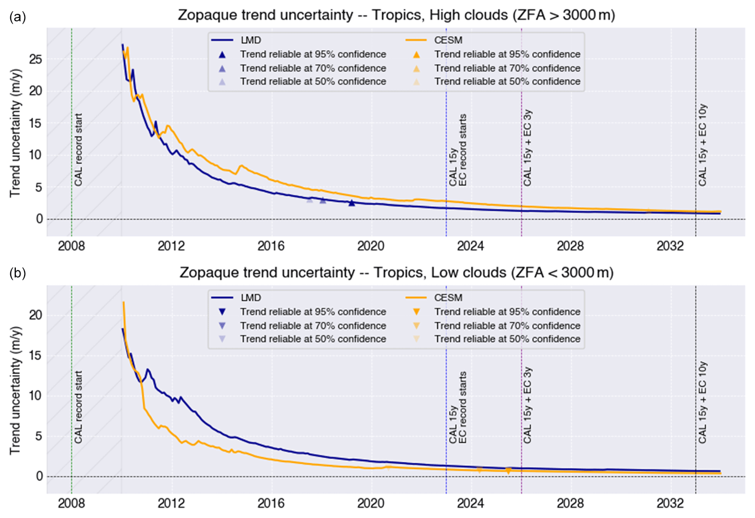
Table C1Variable definitions for the ATLID cloud product. Variables are of the type real (float64) unless specified otherwise. Shaded variables are used as dimensions. L1b: Level 1b.
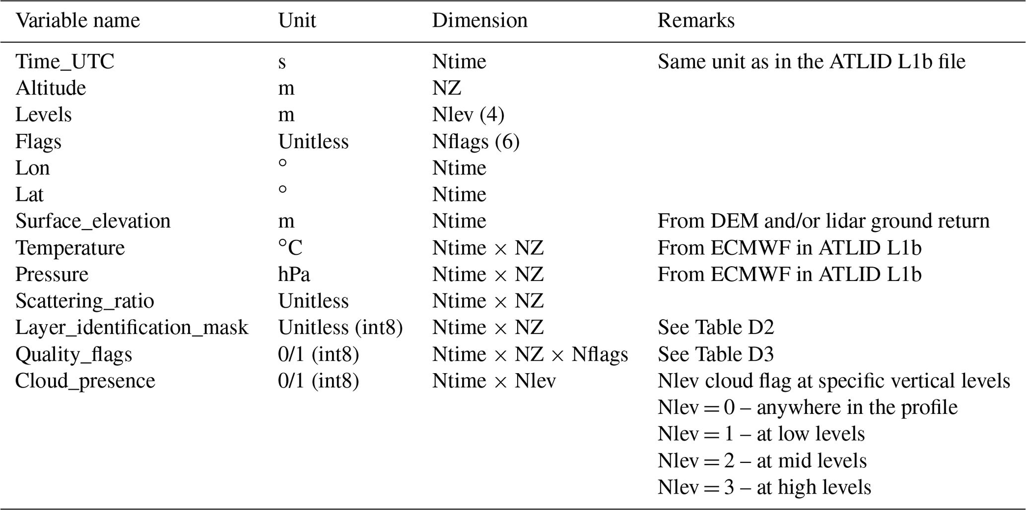
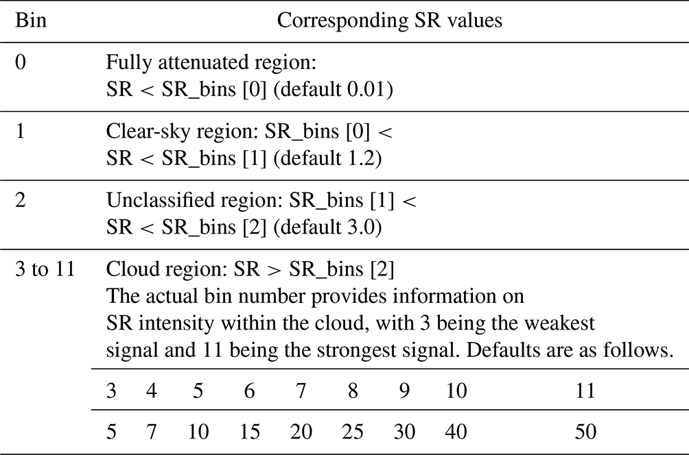
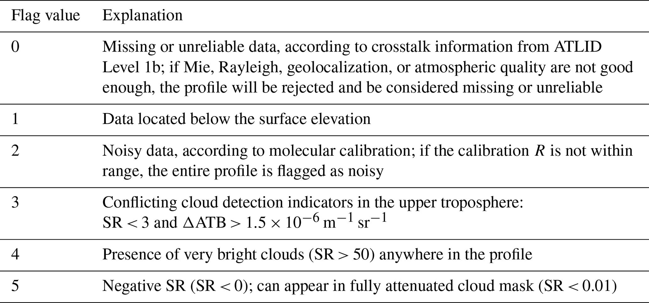
We do not present the code in this work. The “lidar-consistent opaque cloud fractions and altitude of attenuation” dataset used in this work is available for download at https://doi.org/10.5281/zenodo.8059374 (Noel et al., 2023).
HC, VN, and AF: conceptualization, investigation, methodology, and validation. FS: calculation of cloud distributions. AF: data curation and formal analysis. AF: writing of original draft. AF, HC, and VN: review and editing.
The contact author has declared that none of the authors has any competing interests.
Publisher’s note: Copernicus Publications remains neutral with regard to jurisdictional claims in published maps and institutional affiliations.
This article is part of the special issue “EarthCARE Level 2 algorithms and data products”. It is not associated with a conference.
This work was supported by the European Space Agency (ESA) (contract no. 4000xxxxxx/221/I-DT-lr). This work was also supported by the Centre National de la Recherche Scientifique (CNRS) and by the Centre National d'Études Spatiales (CNES) through the Expecting EarthCARE, Learning from A-Train (EECLAT) project as well as by the Office National d'Études et de Recherches Aérospatiales (ONERA, the French Aerospace Lab). The authors want to thank Institut Pascal at Université Paris-Saclay and the organizers of the 4-week Atmospheric Cycle Workshop for inspiring this study (French investissements d'avenir grant no. ANR-11-IDEX-0003-01). Special thanks go to Valery Shcherbakov (Laboratoire de Météorologie Physique, Université Clermont Auvergne, Aubière, France) for discussing the multiple scattering coefficient in relation to CALIOP and ATLID. Lastly, the authors express their gratitude to the reviewers, Sebastian Bley (ESA ESRIN, LITR) and Mark Vaughan (NASA Langley), for their thorough reviews and valuable comments. The authors would like to extend their sincere appreciation to the late Tobias Wehr, who served as the EarthCARE mission scientist at ESA, for his unwavering support of their work in the course of last 10 years.
This work was supported by the European Space Agency (ESA) (contract no. 4000xxxxxx/221/I-DT-lr). This work was also supported by the Centre National de la Recherche Scientifique (CNRS) and by the Centre National d'Études Spatiales (CNES) through the Expecting EarthCARE, Learning from A-Train (EECLAT) project as well as by the Office National d'Études et de Recherches Aérospatiales (ONERA, the French Aerospace Lab).
This paper was edited by Hajime Okamoto and reviewed by Mark Vaughan and Sebastian Bley.
Aerenson, T., Marchand, R., Chepfer, H., and Medeiros, B.: When Will MISR Detect Rising High Clouds? J. Geophys. Res.-Atmos., 127, e2021JD035865, https://doi.org/10.1029/2021JD035865, 2022.
Alkasem A., Szczap, F., Cornet, C., Shcherbakov, V., Gour, Y., Jourdan, O., Labonnote, L. C., and Mioche, G.: Effects of cirrus heterogeneity on lidar CALIOP/CALIPSO data, JQSRT, 202, 38–49, https://doi.org/10.1016/j.jqsrt.2017.07.005, 2017.
Berry, E., Mace, G. G., and Gettelman, A. : Using A-Train Observations to Evaluate Cloud Occurrence and Radiative Effects in the Community Atmosphere Model during the Southeast Asia Summer Monsoon, J. Climate, 32, 4145–4165, https://doi.org/10.1175/JCLI-D-18-0693.1, 2019.
Beyerle, G., Gross, M. R., Haner, D. A., Kjome, N. T., McDermid, I. S., McGee, T. J., Rosen, J. M., Schäfer, H.-J., and Schrems, O.: A Lidar and Backscatter Sonde Measurement Campaign at Table Mountain during February-March 1997: Observations of Cirrus Clouds. J. Appl. Meteor., 40, 1275–1287, https://doi.org/10.1175/1520-0469(2001)058<1275:ALABSM>2.0.CO;2, 2001.
Bodas-Salcedo, A., Webb, M. J., Bony, S., Chepfer, H, J.-l. Dufresne, J.-L., Klein, S. A., Zhang, Y., Marchand, R., Haynes, J. M., Pincus, R., and John, V. O.: COSP, Satellite simulation software for model assessment, B. Am. Meteorol. Soc., 92, 1023–1043, https://doi.org/10.1175/2011BAMS2856.1, 2011.
Boucher, O., Servonnat, J., Albright, A. L., Aumont, O., Balkanski, Y., Bastrikov, V., Bekki, S., Bonnet, R., Bony, S., Bopp, L., Braconnot, P., Brockmann, P., Cadule, P., Caubel, A., Cheruy, F., Codron, F., Cozic, A., Cugnet, D., D'Andrea, F., Davini, P., de Lavergne, C., Denvil, S., Deshayes, J., Devilliers, M., Ducharne, A., Dufresne, J. L., Dupont, E., Éthé, C., Fairhead, L., Falletti, L., Flavoni, S., Foujols, M. A., Gardoll, S., Gastineau, G., Ghattas, J., Grandpeix, J. Y., Guenet, B., Guez, L. E., Guilyardi, E., Guimberteau, M., Hauglustaine, D., Hourdin, F., Idelkadi, A., Joussaume, S., Kageyama, M., Khodri, M., Krinner, G., Lebas, N., Levavasseur, G., Lévy, C., Li, L., Lott, F., Lurton, T., Luyssaert, S., Madec, G., Madeleine, J. B., Maignan, F., Marchand, M., Marti, O., Mellul, L., Meurdesoif, Y., Mignot, J., Musat, I., Ottlé, C., Peylin, P., Planton, Y., Polcher, J., Rio, C., Rochetin, N., Rousset, C., Sepulchre, P., Sima, A., Swingedouw, D., Thiéblemont, R., Traore, A. K., Vancoppenolle, M., Vial, J., Vialard, J., Viovy, N., and Vuichard, N.: Presentation and Evaluation of the IPSL-CM6A-LR Climate Model, J. Adv. Model. Earth Syst., 12, e2019MS002010, https://doi.org/10.1029/2019MS002010, 2020.
Cesana, G., Del Genio, A. D., and Chepfer, H.: The Cumulus And Stratocumulus CloudSat-CALIPSO Dataset (CASCCAD), Earth Syst. Sci. Data, 11, 1745–1764, https://doi.org/10.5194/essd-11-1745-2019, 2019.
Chemke, R.: Future changes in the Hadley circulation: The role of ocean heat transport, Geophys. Res. Lett., 48, e2020GL091372. https://doi.org/10.1029/2020GL091372, 2021.
Cheng, Z., Liu, D., Yang, Y., Yang, L., and Huang, H.: Interferometric filters for spectral discrimination in high-spectral-resolution lidar: performance comparisons between Fabry–Perot interferometer and field-widened Michelson interferometer, Appl. Opt., 52, 7838–7850, https://doi.org/10.1364/AO.52.007838, 2013.
Chepfer, H., Bony, S., Winker, D., Chiriaco, M., Dufresne, J.-L., and Sèze, G.: Use of CALIPSO lidar observations to evaluate the cloudiness simulated by a climate model, Geophys. Res. Let., 35, L15704, https://doi.org/10.1029/2008GL034207, 2008.
Chepfer, H., Bony, S., Winker, D., Cesana, G., Dufresne, J.-L., Minnis, P., Stubenrauch, C. J., and Zeng, S.: The GCM Oriented Calipso Cloud Product (CALIPSO-GOCCP), J. Geophys. Res., 115, D00H16, https://doi.org/10.1029/2009JD012251, 2010.
Chepfer, H., Cesana, G., Winker, D., Getzewich, B., and Vaughan, M.: Comparison of two different cloud climatologies derived from CALIOP Level 1 observations: the CALIPSO-ST and the CALIPSO-GOCCP, J. Atmos. Ocean. Technol., 30, 725–744 https://doi.org/10.1175/JTECH-D-12-00057.1, 2013.
Chepfer, H., Noël, V., Winker, D., and Chiriaco, M.: Where and when will we observe cloud changes due to climate warming?, Geophys. Res. Lett., 41, 8387–8395, https://doi.org/10.1002/2014GL061792, 2014.
Chepfer, H., Noël, V., Chiriaco, M., Wielicki, B., Winker, D., Loeb, N., and Wood, R.: The potential of multi-decades space-born lidar to constrain cloud feedbacks, J. Geophys. Res.-Atmos., 123, 5433–5454, https://doi.org/10.1002/2017JD027742, 2018.
Chepfer, H., Brogniez, H., and Noël, V.: Diurnal variations of cloud and relative humidity profiles across the tropics, Sci. Rep., 9, 16045, https://doi.org/10.1038/s41598-019-52437-6, 2019.
Chiriaco, M., Vautard, R., Chepfer, H., Haeffelin, M., Dudhia, J., Wanherdrick, Y., Morille, Y., and Protat, A.: The Ability of MM5 to Simulate Ice Clouds: Systematic Comparison between Simulated and Measured Fluxes and Lidar/Radar Profiles at the SIRTA Atmospheric Observatory, Mon. Weather Rev., 134, 897–918, https://doi.org/10.1175/MWR3102.1, 2006.
Davis, S. M. and Rosenlof, K. H.: A multidiagnostic intercomparison of tropical-width time series using reanalyses and satellite observations, J. Climate, 25, 1061–1078, 2012.
do Carmo, J. P., Villele, de V., Wallace, K., Lefebvre, A., Ghose, K., Kanitz, T., Chassat, F., Corselle, B., Belhadj, T., and Bravetti, P.: ATmospheric LIDar(ATLID): Pre-launch testing and calibration of the European Space Agency instrument that will measure aerosols and thin clouds in the atmosphere, Atmosphere, 12, 76, https://doi.org/10.3390/atmos12010076, 2021.
Donovan, D. P.: The Expected Impact of Multiple Scattering on ATLID Signals, EPJ Conf., 119, 01006, https://doi.org/10.1051/epjconf/201611901006, 2016.
Durand, Y., Hélière, A., Bézy, J.-L., and Meynart, R.: The ESA EarthCARE mission: Results of the ATLID instrument pre-developments, Proc. SPIE, 6750, 675015, https://doi.org/10.1117/12.737932, 2007.
Eyring, V., Bony, S., Meehl, G. A., Senior, C. A., Stevens, B., Stouffer, R. J., and Taylor, K. E.: Overview of the Coupled Model Intercomparison Project Phase 6 (CMIP6) experimental design and organization, Geosci. Model Dev., 9, 1937–1958, https://doi.org/10.5194/gmd-9-1937-2016, 2016.
Feofilov, A. G. and Stubenrauch, C. J.: Diurnal variation of high-level clouds from the synergy of AIRS and IASI space-borne infrared sounders, Atmos. Chem. Phys., 19, 13957–13972, https://doi.org/10.5194/acp-19-13957-2019, 2019.
Feofilov, A. G., Stubenrauch, C. J., and Delanoë, J.: Ice water content vertical profiles of high-level clouds: classification and impact on radiative fluxes, Atmos. Chem. Phys., 15, 12327–12344, https://doi.org/10.5194/acp-15-12327-2015, 2015.
Feofilov, A. G., Chepfer, H., Noël, V., Guzman, R., Gindre, C., Ma, P.-L., and Chiriaco, M.: Comparison of scattering ratio profiles retrieved from ALADIN/Aeolus and CALIOP/CALIPSO observations and preliminary estimates of cloud fraction profiles, Atmos. Meas. Tech., 15, 1055–1074, https://doi.org/10.5194/amt-15-1055-2022, 2022.
Garnier, A., Pelon, J., Vaughan, M. A., Winker, D. M., Trepte, C. R., and Dubuisson, P.: Lidar multiple scattering factors inferred from CALIPSO lidar and IIR retrievals of semi-transparent cirrus cloud optical depths over oceans, Atmos. Meas. Tech., 8, 2759–2774, https://doi.org/10.5194/amt-8-2759-2015, 2015.
Guzman, R., Chepfer, H., Noël, V., Vaillant de Guelis, T., Kay, J. E., Raberanto, P., Cesana, G., Vaughan, M. A., and Winker, D. M.: Direct atmosphere opacity observations from CALIPSO provide new constraints on cloud-radiation interactions, J. Geophys. Res.-Atmos., 122, 1066–1085, https://doi.org/10.1002/2016JD025946, 2017.
Haynes, J. M., Marchand, R. T., Luo, Z., Bodas-Salcedo, A., and Stephens, G. L.: A multipurpose radar simulation package: QuickBeam, B. Am. Meteorol. Soc., 88, 1723–1727, https://doi.org/10.1175/BAMS-88-11-1723, 2007.
Héliere, A., Gelsthorpe, R., Le Hors, L., and Toulemont, Y.: ATLID, the Atmospheric Lidar on board the EarthCARE Satellite, Proc. SPIE 10564, International Conference on Space Optics – ICSO 2012, 105642D (20 November 2017), https://doi.org/10.1117/12.2309095, 2017.
Heymsfield, A., Krämer, M., Wood, N. B., Gettelman, A., Field, P. R., and Liu, G.: Dependence of the Ice Water Content and Snowfall Rate on Temperature, Globally: Comparison of in Situ Observations, Satellite Active Remote Sensing Retrievals, and Global Climate Model Simulations, J. App. Meteorol. Climatol., 56, 189–215, https://doi.org/10.1175/JAMC-D-16-0230.1, 2017.
Heymsfield, A., Bansemer, A., Wood, N. B., Liu, G., Tanelli, S., Sy, O. O., Poellot, M., and Liu, C.: Toward Improving Ice Water Content and Snow-Rate Retrievals from Radars. Part II: Results from Three Wavelength Radar–Collocated In Situ Measurements and CloudSat–GPM–TRMM Radar Data, J. Appl. Met. Clim., 57, 365–389, https://doi.org/10.1175/JAMC-D-17-0164.1, 2018.
Hogan, R. J. and Illingworth, A. J.: Parameterizing Ice Cloud Inhomogeneity and the Overlap of Inhomogeneities Using Cloud Radar Data, J. Atmos. Sci., 60, 756–767, https://doi.org/10.1175/1520-0469(2003)060<0756:PICIAT>2.0.CO;2, 2003.
Hogan, R. J. and Kew, S.F.: A 3D stochastic cloud model for investigating the radiative properties of inhomogeneous cirrus clouds, Q. J. Roy. Meteorol. Soc., 131, 2585–2608, https://doi.org/10.1256/qj.04.144, 2005.
Hu, Y., Liu, Z., Winker, D., Vaughan, M., Noel, V., Bissonnette, L., Roy, G., and McGill, M.: Simple relation between lidar multiple scattering and depolarization for water clouds, Opt. Lett., 31, 1809–1811, 2006.
Hunt, W. H., Winker, D. M., Vaughan, M. A., Powell, K. A., Lucker, P. L., and Weimer, C.: CALIPSO Lidar Description and Performance Assessment, J. Atmos. Ocean. Technol., 26, 1214–1228, https://doi.org/10.1175/2009JTECHA1223.1, 2009.
Hurrell, J. W., Holland, M. M., Gent, P. R., Ghan, S., Kay, J.E., Kushner, P. J., Lamarque, J.-F., Large, W. G., Lawrence, D., Lindsay, K., Lipscomb, W. H., Long, M. C., Mahowald, N., Marsh, D. R., Neale, R. B., Rasch, P., Vavrus, S., Vertenstein, M., Bader, D., Collins, W. D., Hack, J. J., Kiehl, J., and Marshall, S.: The Community Earth System Model: A Framework for Collaborative Research, B. Am. Meteorol. Soc., 94, 1339–1360, 2013.
Illingworth, A. J., Barker, H. W., Beljaars, A. et al.: The EarthCARE satellite: the next step forward in global measurements of clouds, aerosols, precipitation, and radiation, B. Am. Meteorol. Soc., 96, 1311–1332, https://doi.org/10.1175/BAMS-D-12-00227.1, 2015.
Kärcher, B., Thornberry, T. D., Krämer, M., and Jensen, E. J.: On the statistical distribution of total water in cirrus clouds, Geophys. Res. Lett., 45, 9963–9971, https://doi.org/10.1029/2018GL079780, 2018.
Kingston, R. H.: Detection of Optical and Infrared Radiation, Springer Series in Optical Sciences, v10, Springer, https://doi.org/10.1007/978-3-540-35948-7, 142 pp., 1978.
Kjellsson, J.: Weakening of the global atmospheric circulation with global warming, Clim. Dynam., 45, 975–988, https://doi.org/10.1007/s00382-014-2337-8, 2015.
Klein, S. A. and Jakob, C.: Validation and Sensitivities of Frontal Clouds Simulated by the ECMWF Model, Mon. Weather Rev., 127, 2514–2531, https://doi.org/10.1175/1520-0493(1999)127<2514:VASOFC>2.0.CO;2, 1999.
Konsta, D., Chepfer, H., and Dufresne, J.-L.: A process oriented characterization of tropical oceanic clouds for climate model evaluation, based on a statistical analysis of daytime A-Train observations, Clim. Dynam., 39, 2091–2108, https://doi.org/10.1007/s00382012-1533-7, 2012.
Leahy, L. V., Wood, R., Charlson, R. J., Hostetler, C. A., Rogers, R. R., Vaughan, M. A., and Winker, D. M.: On the nature and extent of optically thin marine low clouds, J. Geophys. Res.-Atmos., 117, D22201, https://doi.org/10.1029/2012JD017929, 2022.
Liu, Z. and Sugimoto, N.: Simulation study for cloud detection with space lidars using analog detection photomultiplier tubes, Appl. Opt., 41, 1750–1759, 2002.
Liu, Z., Hunt, W. H., Vaughan, M., Hostetler, C., McGill, M., Powell, K., Winker, D., and Hu, Y.: Estimating random errors due to shot noise in backscatter lidar observations, Appl. Opt., 45, 4437–4447, https://doi.org/10.1364/AO.45.004437, 2006.
Marchand, R., Haynes, J., Mace, G. G., Ackerman, T., and Stephens, G.: A comparison of simulated cloud radar output from the multiscale modeling framework global climate model with CloudSat cloud radar observations, J. Geophys. Res., 114, D00A20, https://doi.org/10.1029/2008JD009790, 2009.
McGill, M. J., Vaughan, M. A., Trepte, C. R., Hart, W. D., Hlavka, D. L., Winker, D. M., and Kuehn, R.: Airborne validation of spatial properties measured by the CALIPSO lidar, J. Geophys. Res.-Atmos., 112, D20201, https://doi.org/10.1029/2007JD008768, 2007.
McGill, M. J., Yorks, J. E., Scott, V. S., Kupchock, A. W., and Selmer, P. A.: The Cloud-Aerosol Transport System (CATS): A technology demonstration on the International Space Station, Proc. Spie., 9612, https://doi.org/10.1117/12.2190841, 2015.
Nam C., Bony, S., Dufresne, J. L., and Chepfer, H.: The 'too few, too bright' tropical low-cloud problem in CMIP5 models, Geophys. Res. Lett., 39, 21, https://doi.org/10.1029/2012GL053421, 2012.
Noel, V.: Monthly global grids of lidar-consistent opaque cloud fractions and altitude of attenuation 2008–2034 according to predictions from CESM2 and IPSL-CM6 GCMs, Zenodo [data set], https://doi.org/10.5281/zenodo.8059374, 2023.
Noel, V., Chepfer, H., Chiriaco, M., and Yorks, J.: The diurnal cycle of cloud profiles over land and ocean between 51∘ S and 51∘ N, seen by the CATS spaceborne lidar from the International Space Station, Atmos. Chem. Phys., 18, 9457–9473, https://doi.org/10.5194/acp-18-9457-2018, 2018.
Perpina, M., Noel, V., Chepfer, H., Guzman, R., and Feofilov, A. G.: Link between opaque cloud properties and atmospheric dynamics in observations and simulations of current climate in the Tropics, and impact on future predictions. J. Geophys. Res.-Atmos., 126, e2020JD033899. https://doi.org/10.1029/2020JD033899, 2021.
Platt, C. M. R.: Lidar and radiometric observations of cirrus clouds, J. Atmos. Sci., 30, 1191–1204, 1973.
Rasch, P. J., Xie, S., Ma, P.-L., Lin, W., Wang, H., Tang, Q., Burrows, S. M., Caldwell, P., Zhang, K., Easter, R. C., Cameron-Smith, P., Singh, B., Wan, H., Golaz, J.-C., Harrop, B. E., Roesler, E., Bacmeister, J., Larson, V. E., Evans, K. J., Qian, Y., Taylor, M., Leung, L. R., Zhang, Y., Brent, L., Branstetter, M., Hannay, C., Mahajan, S., Mametjanov, A., Neale, R., Richter, J. H., Yoon, J.-H., Zender, C. S., Bader, D., Flanner, M., Foucar, J. G., Jacob, R., Keen, N., Klein, S. A., Liu, X., Salinger, A. G., Shrivastava, M., and Yang, Y.: An Overview of the Atmospheric Component of the Energy Exascale Earth System Model, J. Adv. Model. Earth Syst., 11, 2377–2411, https://doi.org/10.1029/2019MS001629, 2019.
Reitebuch, O., Lemmerz, C., Lux, O., Marksteiner, U., Rahm, S., Weiler, F., Witschas, B., Meringer, M., Schmidt, K., Huber, D., Nikolaus, I., Geiss, A., Vaughan, M., Dabas, A., Flament, T., Stieglitz, H., Isaksen, L., Rennie, M., de Kloe, J., Marseille, G.-J., Stoffelen, A., Wernham, D., Kanitz, T., Straume, A.-G., Fehr, T., von Bismarck, J., Floberghagen, R., and Parrinello, T.: Initial Assessment of the Performance of the First Wind Lidar in Space on Aeolus, EPJ Web Conf., 237, 01010, https://doi.org/10.1051/epjconf/202023701010, 2020.
Reverdy M., Chepfer, H., Donovan, D., Noël, V., Cesana, G., Hoareau, C., Chiriaco, M., and Bastin, S.: An EarthCARE/ATLID simulator to evaluate cloud description in climate models, J. Geophys. Res.-Atmos., 120, 11090–11113, https://doi.org/10.1002/2015JD023919, 2015.
Richardson, M. T., Roy, R. J., and Lebsock, M. D.: Satellites Suggest Rising Tropical High Cloud Altitude: 2002–2021, Geophys. Res. Lett., 49, e2022GL098160, https://doi.org/10.1029/2022GL098160, 2022.
Rogers, R. R., Vaughan, M. A., Hostetler, C. A., Burton, S. P., Ferrare, R. A., Young, S. A., Hair, J. W., Obland, M. D., Harper, D. B., Cook, A. L., and Winker, D. M.: Looking through the haze: evaluating the CALIPSO level 2 aerosol optical depth using airborne high spectral resolution lidar data, Atmos. Meas. Tech., 7, 4317–4340, https://doi.org/10.5194/amt-7-4317-2014, 2014.
Sassen, K. and Comstock, J. M.: A midlatitude cirrus cloud climatology from the facility for atmospheric remote sensing. Part III: Radiative properties, J. Atmos. Sci., 58, 2113–2127, https://doi.org/10.1175/1520-0469(2001)058<2113:Amcccf>2.0.Co;2, 2001.
Schwalm, C. R., Glendon, S., and Duffy, P. B.: RCP85 tracks cumulative CO2 emissions, P. Natl. Acad. Sci. USA, 117, 19656–19657, https://doi.org/10.1073/pnas.2007117117, 2020.
Shcherbakov, V., Szczap, F., Alkasem, A., Mioche, G., and Cornet, C.: Empirical model of multiple-scattering effect on single-wavelength lidar data of aerosols and clouds, Atmos. Meas. Tech., 15, 1729–1754, https://doi.org/10.5194/amt-15-1729-2022, 2022.
Stevens, B., H-Moeng, C., Ackerman A. S., Bretherton, C. S., Chlond, A., de Roode, S., Edwards, J., Golaz, J. C., Jiang, H., Khairoutdinov, M., Kirkpatrick, M. P., Lewellen, D. C., Lock, A. L., Müller, F., Stevens, D. E., Whelan, E., and Zhu, P.: Evaluation of large-eddy simulations via observations of nocturnal marine stratocumulus, Mon. Weather Rev., 133, 1443–1462, 2005.
Straume, A. G., Rennie, M., Isaksen, L., de Kloe, J., Marseille, G.-J., Stoffelen, A., Flament, T., Stieglitz, H., Dabas, A., Huber, D., Reitebuch, O., Lemmerz, C., Lux, O., Marksteiner, U., Weiler, F., Witschas, B., Meringer, M., Schmidt, K., Nikolaus, I., Geiss, A., Flamant, P., Kanitz, T., Wernham, D., von Bismarck, J., Bley, S., Fehr, T., Floberghagen, R., and Parrinello, T.: ESA's Space-Based Doppler Wind Lidar Mission Aeolus – First Wind and Aerosol Product Assessment Results, EPJ Web Conf. 237, 01007, https://doi.org/10.1051/epjconf/202023701007, 2020.
Su, H., Jiang, J. H., Zhai, C., Shen, T. J., Neelin, J. D., Stephens, G. L., and Yung, Y. L: Weakening and strengthening structures in the Hadley Circulation change under global warming and implications for cloud response and climate sensitivity: Circulation, Clouds, Climate Sensitivity, J. Geophys. Res.-Atmos., 119, 5787–5805. https://doi.org/10.1002/2014JD021642, 2014.
Swales, D. J., Pincus, R., and Bodas-Salcedo, A.: The Cloud Feedback Model Intercomparison Project Observational Simulator Package: Version 2, Geosci. Model Dev., 11, 77–81, https://doi.org/10.5194/gmd-11-77-2018, 2018.
Szczap, F., Gour, Y., Fauchez, T., Cornet, C., Faure, T., Jourdan, O., Penide, G., and Dubuisson, P.: A flexible three-dimensional stratocumulus, cumulus and cirrus cloud generator (3DCLOUD) based on drastically simplified atmospheric equations and the Fourier transform framework, Geosci. Model Dev., 7, 1779–1801, https://doi.org/10.5194/gmd-7-1779-2014, 2014.
Takahashi, H., Lebsock, M. D., Richardson, M., Marchand, R., and Kay, J. E.: When Will Spaceborne Cloud Radar Detect Upward Shifts in Cloud Heights?, J. Geophys. Res.-Atmos., 124, 2018JD030242, https://doi.org/10.1029/2018JD030242, 2019.
Vaillant de Guélis, T., Chepfer, H., Noel, V., Guzman, R., Dubuisson, P., Winker, D. M., and Kato, S.: The link between outgoing longwave radiation and the altitude at which a spaceborne lidar beam is fully attenuated, Atmos. Meas. Tech., 10, 4659–4685, https://doi.org/10.5194/amt-10-4659-2017, 2017.
Vaillant de Guélis T., H. Chepfer, Noël, V., Guzman, R., Bonazzola, M., and Winker, D. M.: Space lidar observations constrain longwave cloud feedback, Nature Sci. Rep., 8, 16570, https://doi.org/10.1038/s41598-018-34943-1, 2018.
Voudouri, K. A., Giannakaki, E., Komppula, M., and Balis, D.: Variability in cirrus cloud properties using a PollyXT Raman lidar over high and tropical latitudes, Atmos. Chem. Phys., 20, 4427–4444, https://doi.org/10.5194/acp-20-4427-2020, 2020.
Waliser, D., Gleckler, P. J., Ferraro, R., Taylor, K. E., Ames, S., Biard, J., Bosilovich, M. G., Brown, O., Chepfer, H., Cinquini, L., Durack, P. J., Eyring, V., Mathieu, P.-P., Lee, T., Pinnock, S., Potter, G. L., Rixen, M., Saunders, R., Schulz, J., Thépaut, J.-N., and Tuma, M.: Observations for Model Intercomparison Project (Obs4MIPs): status for CMIP6, Geosci. Model Dev., 13, 2945–2958, https://doi.org/10.5194/gmd-13-2945-2020, 2020.
Winker, D. M., Pelon, J., Coakley Jr., J. A., Ackerman, S. A., Charlson, R. J., Colarco, P. R., Flamant, P., Fu, Q., Hoff, R. M., Kittaka, C., Kubar, T. L., Le Treut, H., Mccormick, M. P., Mégie, G., Poole, L., Powell, K., Trepte, C., Vaughan, M. A., and Wielicki, B. A.: The CALIPSO Mission, A Global 3D View of Aerosols and Clouds, B. Am. Meteor. Soc., 91, 1211–1230, https://doi.org/10.1175/2010BAMS3009.1, 2010.
Winker, D., Chepfer, H., Noël, V., and Cai, X.: Observational constraints on cloud feedbacks: The role of active satellite sensors, Surv. Geophys., 38, 1483–1508, https://doi.org/10.1007/s10712-017-9452-0, 2017.
Young, S. A., Vaughan, M. A., Garnier, A., Tackett, J. L., Lambeth, J. D., and Powell, K. A.: Extinction and optical depth retrievals for CALIPSO's Version 4 data release, Atmos. Meas. Tech., 11, 5701–5727, https://doi.org/10.5194/amt-11-5701-2018, 2018.
Zelinka, M. D., Klein, S. A., and Hartmann, D. L.: Computing and Partitioning Cloud Feedbacks Using Cloud Property Histograms. Part II: Attribution to Changes in Cloud Amount, Altitude, and Optical Depth, J. Climate, 25, 3736–3754, https://doi.org/10.1175/JCLI-D-11-00249.1, 2012.
Zelinka, M. D., Zhou, C., and Klein, S. A.: Insights from a refined decomposition of cloud feedbacks, Geophys. Res. Lett., 43, 9259–9269, https://doi.org/10.1002/2016GL069917, 2016.
Zelinka, M. D., Myers, T. A., McCoy, D. T., Po-Chedley, S., Caldwell, P. M., Ceppi, P., Klein, S. A., and Taylor, K. E.: Causes of higher climate sensitivity in CMIP6 models, Geophys. Res. Lett., 47, e2019GL085782, https://doi.org/10.1029/2019GL085782, 2020.
- Abstract
- Introduction
- Two spaceborne lidars, lidar equation, and cloud detection
- The CLIMP short-term dataset
- The CLIMP long-term dataset
- Conclusions
- Appendix A
- Appendix B
- Appendix C
- Code and data availability
- Author contributions
- Competing interests
- Disclaimer
- Special issue statement
- Acknowledgements
- Financial support
- Review statement
- References