2.1 L₂ regularization

2.2 Computing the design matrix

The design matrix can be obtained from a forward model

where y is a vector representing the error-free observations, x is the vector of true inputs, c is a vector of controlling parameters, and F is the linear forward model function that maps over x to compute y subject to the constraint of c. The matrix of the linear transformation y=Ax is then given by

where ${\mathit{e}}_{\mathrm{1}},\mathrm{\dots },{\mathit{e}}_{\text{n}}$ is the standard basis. RegularizationTools.jl also provides an abstract generic interface that simplifies computation of the design matrix from arbitrary forward models of linear processes. Examples demonstrating how to use this generic interface are provided in the documentation of the package. The examples include the solution for transit through the tandem DMA described further below, the solution of the Fredholm integral equation of the first kind given by Baart (1982), the optical convolution that underlies size distribution retrieval from scattering and absorption properties (Müller et al., 2019), and the 2D Gaussian blur function encountered in image processing.

2.3 Design matrices for differential mobility analyzers

Differential mobility analyzers consist of two electrodes held at a constant or time-varying electric potential. Cylindrical (Knutson and Whitby, 1975) and radial (Zhang et al., 1995; Russell et al., 1996) electrode geometries are the most common. Charged particles in a flow between the electrodes are deflected to an exit slit and measured by a suitable detector, usually a condensation particle counter. The fraction of particles carrying k charges is described by a statistical distribution that is created by the charge conditioner used upstream of the DMA. The functions governing the transfer through bipolar charge conditioners, single DMAs, and tandem DMAs are well understood (Knutson and Whitby, 1975; Rader and McMurry, 1986; Reineking and Porstendörfer, 1986; Wang and Flagan, 1990; Stolzenburg and McMurry, 2008; Jiang et al., 2014).

The DMA selects particles by electrical mobility. The relationship between mobility and mobility diameter is well known and well defined. The relationship is given, for example, in Eq. (2) in Petters (2018). This work also makes use of the “apparent + 1 mobility diameter”. It is defined as the conversion from mobility to diameter assuming singly charged particles using the mobility grid scanned by either DMA 1 or DMA 2. The apparent + 1 mobility diameter represents the natural diameter axis of a DMA response function, i.e., a plot of the raw detector response versus the nominal DMA setpoint diameter. It is an equivalent measure of mobility. The apparent + 1 mobility diameter is ambiguous. Larger particles carrying more than one charge may have the same apparent + 1 mobility diameter as smaller particles carrying fewer charges. The “apparent growth factor” is defined as the apparent + 1 mobility diameter scanned by DMA 2 divided by the nominal selected dry diameter in the DMA.

The traditional mathematical formulation of transfer through the DMA is summarized in Stolzenburg and McMurry (2008) and references therein. Briefly, the integrated response downstream of the DMA operated at voltage V₁ is given by a single integral that includes a summation over all selected charges. The size distribution is measured by varying voltage V₁, which produces the raw response function defined as the integrated response downstream of the DMA as a function of upstream voltage. The size distribution is found by inversion. The basic mathematical problem associated with inverting the response function to find the size distribution is summarized by Kandlikar and Ramachandran (1999). The integral is discretized by quadrature to find the design matrix that maps the size distribution to the response function. L₂ regularization is one of several methods to reconstruct the size distribution from the response function (Voutilainen et al., 2001; Kandlikar and Ramachandran, 1999).

The integrated response downstream of a tandem DMA that is operated at voltages V₁ and V₂ requires evaluating integrals of the upstream particle size distribution over size and the grown particle size distribution over size. The integration must be repeated for each charge state. Scanning over a range of voltages V₂ results in the raw tandem DMA response function. For the forward calculation, the objective is to find a design matrix that maps the growth factor frequency distribution to the raw TDMA response function.

Petters (2018) introduced a computational approach to model transfer through the DMA. The main idea of the approach is to provide a domain-specific language comprising a set of simple building blocks that can be used to algebraically express the response functions intuitively through a form of pseudo-code. The main advantage of this approach is that the expressions simultaneously encode the theory governing the transfer through the DMA and the algorithmic solution to compute the response function. The resulting expressions are concise. They are easily identified within actual source code when working through the examples provided with the package documentation. This makes the code easily modifiable by non-experts to change existing terms or add new convolution terms without the need to develop algorithms.

A disadvantage of the computational approach compared to the traditional mathematical approach is that computation lacks standardization of notation. This can blur the line between general pseudo-code and language-specific syntax. Some of the applied computing concepts may be less widely known when compared to standard mathematical approaches. Nevertheless, the author believes that the advantages of the computational approach outweigh the drawbacks. Therefore, this work builds upon the expressions reported in Petters (2018). Updates and clarifications to the earlier work are noted where appropriate.

The computational language includes a standardized representation of aerosol size distributions, operators to construct expressions, and functions to evaluate the expressions. Size distributions are represented as a histogram and internally stored in the form of the SizeDistribution composite data type. Composite data types combine multiple arrays into a single symbol for ease of use, thus facilitating faster experimental design and analysis. The size distribution data type SizeDistribution includes vectors of the selected mobility bins considered by the DMA, +1 mobility diameter bin edges and +1 mobility diameter bin midpoints computed from the mobility grid, number concentration, log-normalized spectral density, and logarithmic bin widths. SizeDistributions are denoted in blackboard bold font (e.g., 𝕟, 𝕣). SizeDistributions are the building block of composable algebraic expressions through operators that evaluate to transformed SizeDistributions. For example, 𝕟₁+𝕟₂ is the superposition of two size distributions, a⋅𝕟 is the uniform scaling of the concentration fields by factor a, A⋅𝕟 is the matrix multiplication of A and concentration fields of the size distribution, and T⋅𝕟 is the elementwise scaling of the diameter field by factor T. (Note that Petters, 2018, used T. ⋅ 𝕟 as the elementwise scaling. The extra dot has been dropped to stay consistent with the current software implementation.)

Generic functions are used to evaluate expressions. The function $\sum (f,m)$ evaluates the function f(x) for $x=[\mathrm{1},\mathrm{\dots },m]$ and sums the results. If f(x) evaluates to a vector, the sum is the sum of the vectors. The function map(f,x) applies f(x) to each element of vector x and returns a vector of results in the same order. The function foldl(f,x) applies the bivariate function f(a,x) to each element of x and accumulates the result, where a represents the accumulated value. If no initial value is provided, as is the case in this paper, foldl applies the function to the first two elements of the list to compute the first a. For example $\mathrm{foldl}(-,[\mathrm{1},\mathrm{2},\mathrm{3}\left]\right)$ evaluates the function $-(a,x)$ and yields $\mathrm{1}-\mathrm{2}-\mathrm{3}=-\mathrm{4}$. The function $\mathrm{mapfoldl}(f,g,x)$ combines map and foldl. It applies function f to each element in x such that y=f(x) and then reduces the result using the bivariate function g(a,y), where a represents the accumulated value. For example, $\text{mapfoldl(sqrt},-,[\mathrm{4},\mathrm{16},\mathrm{64}])$ evaluates to $\mathrm{foldl}(-,[\mathrm{2},\mathrm{4},\mathrm{8}\left]\right)=\mathrm{2}-\mathrm{4}-\mathrm{8}=-\mathrm{10}$. The function vcat(x,y) concatenates arrays x and y along the first dimension in Julia. However, other programming languages may concatenate along a different dimension as the definition of horizontal and vertical is arbitrary. Passing vcat to foldl (or mapfoldl) will result in a concatenated array. Anonymous functions are used as arguments of reducing functions. Anonymous functions are denoted as x→expression, where x is the argument consumed in the evaluation of the expression. These functions are generic and represent widely used computing concepts. They are implemented in most modern programming languages.

DMA geometry, dimensions, and configuration are abstracted into composite types Λ (configuration comprising flow rates, power supply polarity, and thermodynamic state) and δ (DMA domain defined by a mobility–size grid). Each DMA is fully described by a pair Λ,δ. Subscripts and superscripts are used to distinguish between different configurations in chained DMA setups, e.g., with δ₁ and δ₂ denoting the first and second DMA, respectively. Application of size distribution expressions to transfer functions constructs a concise model of the transmitted DMA mobility distribution, denoted as the DMA response function. Implementation of the language is distributed through a freely available and independently documented package DifferentialMobilityAnalyzers.jl, written in the Julia language. Expressions in the text are provided in general mathematical form for readability.

Petters (2018) gives a simple expression that models transfer through the DMA. The function $T_{\text{size}}^{\mathrm{\Lambda },\mathit{\delta }}(k,z^{\text{s}})$ evaluates to a vector representing the fraction of particles carrying k charges that exit DMA^Λ,δ as a function of mobility

where z^s is the centroid mobility selected by the DMA (determined by the voltage and DMA geometry), Z is a vector of particle mobilities, Ω is the diffusing DMA transfer function (Stolzenburg and McMurry, 2008), T_c is the charge frequency distribution function (Wiedensohler, 1988), and T_l is the diameter-dependent penetration efficiency function (Reineking and Porstendörfer, 1986). The diameter ${\mathit{D}}_{p,\mathrm{1}}=D_p(\mathit{Z},k=\mathrm{1})$ and evaluates to a vector of diameters. The function Ω has been updated from Petters (2018). The version in Petters (2018) computed the shape of the transfer function for the mobility diameter corresponding to singly charged particles and then applied the same shape of the transfer function and diffusional loss to the multiply charged particles. The functional Ω depends on three arguments $\mathrm{\Omega }(\mathit{Z},z^{\text{s}},k)$ and implicitly on the DMA configuration Λ (i.e., Eq 13 in Stolzenburg and McMurry, 2008). The output is a vector along the mobility grid Z. The maximum transmission occurs at $\mathit{Z}/z^{\text{s}}=\mathrm{1}$. The last argument denotes the number of charges. It is used to compute the mobility diameter from z^s and in turn the diffusion coefficient which is required to account for diffusional broadening of the transfer function. The output of $T_{\text{size}}^{\mathrm{\Lambda },\mathit{\delta }}(k,z^{\text{s}})$ is the transmission of particles through the DMA in terms of the true particle mobility diameter. This is achieved by passing $z^{\text{s}}/k$ as an argument of Ω, which corresponds to the centroid mobility setting for the DMA to transmit particles with k charges under the assumption that they carry only a single charge. The net result is that ${\mathit{D}}_{p,\mathrm{1}}=D_p(\mathit{Z},k=\mathrm{1})$ becomes equal to the true mobility diameter axis. As a consequence the charge fraction $T_{\text{c}}(k,{\mathit{D}}_{p,\mathrm{1}})$ and penetration efficiency T_l(D_p,1) are evaluated at the correct diameter. The function $T_{\text{size}}^{\mathrm{\Lambda },\mathit{\delta }}(\mathrm{1},z^{\text{s}})$ evaluates to a vector of the same length as Z. Performing an elementwise sum over all $T_{\text{size}}^{\mathrm{\Lambda },\mathit{\delta }}(k,z^{\text{s}})$ (where the sum is over all charges k) produces the net transmission probability function. Multiplication of the transmission probability function with the input distribution results in the mobility distribution transmitted by the DMA. Examples for $T_{\text{size}}^{\mathrm{\Lambda },\mathit{\delta }}(\mathrm{1},z^{\text{s}})\cdot \mathbb{n}$, $T_{\text{size}}^{\mathrm{\Lambda },\mathit{\delta }}(\mathrm{2},z^{\text{s}})\cdot \mathbb{n}$, and $T_{\text{size}}^{\mathrm{\Lambda },\mathit{\delta }}(\mathrm{3},z^{\text{s}})\cdot \mathbb{n}$ are shown in Fig. 2, right panel, in Petters (2018). Note that Eq. (10) can be evaluated using arbitrarily discretized Z vectors.

Petters (2018) also gives an expression that evaluates to the convolution matrix for passage through a single DMA that is valid in the context of the size distribution measurement system, e.g., SMPS. Since the expression includes a summation over all charges, the information on the particle physical diameter of multiply charged particles is lost.

where m is the upper number of multiply charged particles, ^T is the transpose operator, and Z_s is a vector of centroid mobilities scanned by the DMA. The matrix is square if Z_s=Z in Eq. (11). However, this is not a necessary restriction. Equation (11) evaluates to the same as Eq. (8) in Petters (2018), but the notation is revised to be more general by removing the Julia-specific splatting construct and replacing it with more widely used generic functions.

To help with parsing the expression, $T_{\text{size}}^{\mathrm{\Lambda },\mathit{\delta }}(k,z^{\text{s}})$ evaluates to a vector of transmission for k charges and setpoint centroid mobility z^s as a function of the entire mobility grid (e.g., 120 bins discretized between mobility z₁ and z₂). The function $\mathrm{\Sigma }[k\to T_{\text{size}}^{\mathrm{\Lambda },\mathit{\delta }}(k,z^{\text{s}}),m]$ superimposes the vectors for all charges. Mapping $z^{\text{s}}\to \mathrm{\Sigma }[k\to T_{\text{size}}^{\mathrm{\Lambda },\mathit{\delta }}(k,z^{\text{s}}),m]$ over the centroid mobility grid Z_s produces an array of vectors, each corresponding to the transmission for a single size bin. Transposing the vectors and reducing the collection through concatenation produces the design matrix that links the mobility size distribution to the response function; i.e.,

where 𝕣 is the response distribution, 𝕟 is the true mobility size distribution, and ϵ is a vector denoting the random error that may be superimposed as a result of measurement uncertainties. By design 𝕟 and 𝕣 are SizeDistribution objects, which represent the distribution as a histogram in both spectral density units ($\mathrm{d}N/\mathrm{d}\ln D$) and concentration-per-bin units. The latter is the raw response function, where each element corresponds to the integrated response downstream of DMA 1 for a set upstream voltage (or corresponding z^s or apparent + 1 mobility diameter but not true physical diameter for multiply charged particles). Note, however, that the response function is not a true particle size distribution in the scientific sense since information about multiply charged particles is lost. The representation of 𝕣 as a SizeDistribution object is to allow response functions to be used in the expression-based framework used here.

The mobility distribution exiting the humidity conditioner and before entering DMA 2 in the humidified tandem DMA is evaluated using the expression

where $g_{\mathrm{0}}=D_{\text{wet}}/D_{\text{dry}}$ is the diameter growth factor, D_dry is the selected diameter by DMA 1, D_wet is the diameter after the humidifier, $T_{\text{size}}^{{\mathrm{\Lambda }}_{\mathrm{1}},{\mathit{\delta }}_{\mathrm{1}}}(k,z^{\text{s}})$ is as in Eq. (10), and 𝕟 is the mobility size distribution upstream of DMA 1. Subscripts are used to differentiate DMA 1 and 2 which possibly have different geometries, flow rates, thermodynamic states, and mobility grids, e.g., Λ₁, Λ₂ and δ₁, δ₂. To help parse Eq. (13), the product $T_{\text{size}}^{{\mathrm{\Lambda }}_{\mathrm{1}},{\mathit{\delta }}_{\mathrm{1}}}(k,z^{\text{s}})\cdot \mathbb{n}$ evaluates to the transmitted mobility distributions of particles carrying k charges at the setpoint mobility z^s in DMA 1. The size distribution is grown by the growth factor g₀, which is achieved by applying the ⋅ operator to the product $T_{\text{size}}^{{\mathrm{\Lambda }}_{\mathrm{1}},{\mathit{\delta }}_{\mathrm{1}}}(k,z^{\text{s}})\cdot \mathbb{n}$. Equation (13) assumes that g₀ applies to all particle sizes.

The total humidified apparent + 1 mobility diameter distribution ${\mathbb{m}}_{\text{t}}^{{\mathit{\delta }}_{\mathrm{2}}}$ exiting DMA 2 is given by

where m is upper number of charges on the multiply charged particles and

is the convolution matrix for transport through DMA 2 and particles carrying k charges. In Eq. (15), Z_s,2 is a vector of centroid mobilities scanned by DMA 2. Note that the choice of Z inside Ω is up to the user. Sensible choices are $\mathit{Z}={\mathit{Z}}_{s,\mathrm{1}}$ or Z=Z_s,2, the implications of which are further discussed later. Equations (14) and (15) have been modified from those in Petters (2018) in the following manner. The convolution matrix O_k is computed individually for each charge. The version in Petters (2018) computed the matrix corresponding to singly charged particles and then applied the same matrix to multiply charged particles. Since O_k is now charge resolved, it is moved into the summation in Eq. (14). Computation of O_k through Eq. (15) has been revised to be more general by removing a Julia-language-specific construct. O₁ computed by Eq. (15) produces the same matrix as in Petters (2018). The resulting ${\mathbb{m}}_{\text{t}}^{{\mathit{\delta }}_{\mathrm{2}}}$ size distribution represents the apparent + 1 mobility diameter scanned by DMA 2. Equations (13)–(15) relax an approximation made in a similar treatment in Petters (2018). There it was assumed that the apparent + 1 mobility diameter (and thus apparent growth factor) for particles carrying multiple charges is the same as for singly charged particles. This is incorrect. Particles carrying more than a single charge alias at a smaller particle size (Gysel et al., 2009; Shen et al., 2021). The effect is due to the size dependence of the slip-flow correction factor and is captured by the revised charge-resolved convolution matrices O_k.

If the aerosol is externally mixed, the humidified apparent growth factor distribution function exiting DMA 2 is given by

where P_g is the growth factor probability density function and the diameters resulting from the intermediate calculation ${\sum }_{k=\mathrm{1}}^m\left({\mathbf{O}}_{\text{k}}\cdot {\mathbb{M}}_{\text{k}}^{{\mathit{\delta }}_{\mathrm{1}}}\right)$ are normalized by D_dry. ${\mathbb{m}}_{\text{t}}^{{\mathit{\delta }}_{\mathrm{2}}}$ in Eq. (16) is the forward model through the tandem DMA. Using the notation in Sect. 2.2,

where x is the discrete representation of the true P_g and the vector c of constraining parameters comprises the DMA setups ${\mathrm{\Lambda }}_{\mathrm{1}},{\mathrm{\Lambda }}_{\mathrm{2}},{\mathit{\delta }}_{\mathrm{1}}$, and δ₂ and upstream size distribution 𝕟. Computer code that creates a forward model for tandem DMAs has been added to the DifferentialMobiltyAnalyzers.jl package and is annotated in the documentation of the package.

For purposes of the forward model, the mobility grid for DMA 1 is discretized at a resolution of i bins by specifying the Z vector in Eq. (10). If the Z vector does not match that of the aerosol size distribution 𝕟, the size distribution bins are interpolated onto the diameter bins corresponding to the Z bins. Transmission through DMA 1 is computed for a specified z^s (the dry mobility) and g₀ (the growth factor) via Eq. (13). The resulting ${\mathbb{M}}_{\text{k}}^{{\mathit{\delta }}_{\mathrm{1}}}$ lies on the same Z grid with i bins. Any mismatches between the apparent growth factor and the underlying Z grid are resolved via interpolation implicit in the ⋅ operator. (f⋅𝕟 is the uniform scaling of the diameter field of the size distribution by factor f. If the resulting diameters are off the original diameter grid, the result is interpolated onto the grid defined within 𝕟.) The mobility grid for DMA 2 is represented by the vector Z_s,2 in Eq. (15) and discretized at a resolution of j bins over a custom mobility range. If the vector Z inside the square brackets of Eq. (15) $\left[{\mathrm{\Omega }}^{{\mathrm{\Lambda }}_{\mathrm{2}},{\mathit{\delta }}_{\mathrm{2}}}\right(\mathit{Z},z^{\text{s}}/k,k).\cdot T_l^{{\mathrm{\Lambda }}_{\mathrm{2}},{\mathit{\delta }}_{\mathrm{2}}}({\mathit{D}}_{p,\mathrm{1}}\left)\right]$ equals that of DMA 1, the product ${\mathbf{O}}_{\text{k}}\cdot {\mathbb{M}}_{\text{k}}^{{\mathit{\delta }}_{\mathrm{1}}}$ will map the i bins from DMA 1 to the j bins in DMA 2. Alternatively, if the Z vector inside the square brackets of Eq. (15) is taken to be equal to Z_s,2, the matrices O_k are square and of dimension j×j. In that case, the transmitted and grown distribution from DMA 1 (i bins along the mobility axis of DMA 1) is interpolated onto the mobility grid of DMA 2 prior to evaluating ${\mathbf{O}}_{\text{k}}\cdot {\mathbb{M}}_{\text{k}}^{{\mathit{\delta }}_{\mathrm{1}}}$. The advantage of this approach is that for j<i, the matrices O_k are smaller and subsequent calculations are faster. The forward model, defined by Eq. (14), can be evaluated for arbitrary g₀ values. Thus the growth factor probability distribution P_g in Eq. (17) can be discretized into n arbitrary growth factor bins. A natural choice is to accept growth factor values that coincide with the mobility grid of DMA 2; i.e., the bins align with $\mathit{g}={\mathit{D}}_{p,\mathrm{1}}/D_{\text{d}}$, where D_d is the nominal diameter selected by DMA 1, D_p,1 is equal to $D_p(\mathit{Z},k=\mathrm{1})$. However, this is not required for evaluating Eq. (17). Equation (17) is cast into matrix form such that the humidified mobility distribution function is given by

where the matrix B is understood to be computed for a specific input aerosol size distribution and ϵ is a vector that denotes the random error that may be superimposed as a result of measurement uncertainties. If the grids used to represent the growth factor distribution and that of DMA 2 do not align, interpolation is used to map the growth factor bins from the growth factor distribution onto those corresponding to the DMA 2 grid. The choice of i, j, and n, the ranges of mobility grids for DMA 1 and DMA 2 and the range of the growth grid for P_g, is only constrained by computing resources and a physically reasonable representation of the problem domain. Reasonable choices are i=120 and $j=n=\mathrm{60}$, where the range in apparent growth factor spans $\mathrm{0.8}<\mathit{g}<\mathrm{5.0}$. The size of B is j×n. Uncertainties in the size distribution propagate into B. The main influence of the error will be the relative fraction of +1, +2, and +3 charged particles. Assuming a random error of ± 20 % in concentration, the overall effect on ${\mathbb{m}}_{\text{t}}^{{\mathit{\delta }}_{\mathrm{2}}}$ is expected to be small. Note that interpolation is widely used in this framework. Interpolation may affect how errors propagate through the model. Interpolation in Eq. (13) is unavoidable. However, interpolation can be minimized by working with non-square O_k and matching the grid of P_g to that of DMA 2. Informal tests working with different binning schemes suggest that the influence of interpolation choices on the final result is smaller than typical experimental errors.

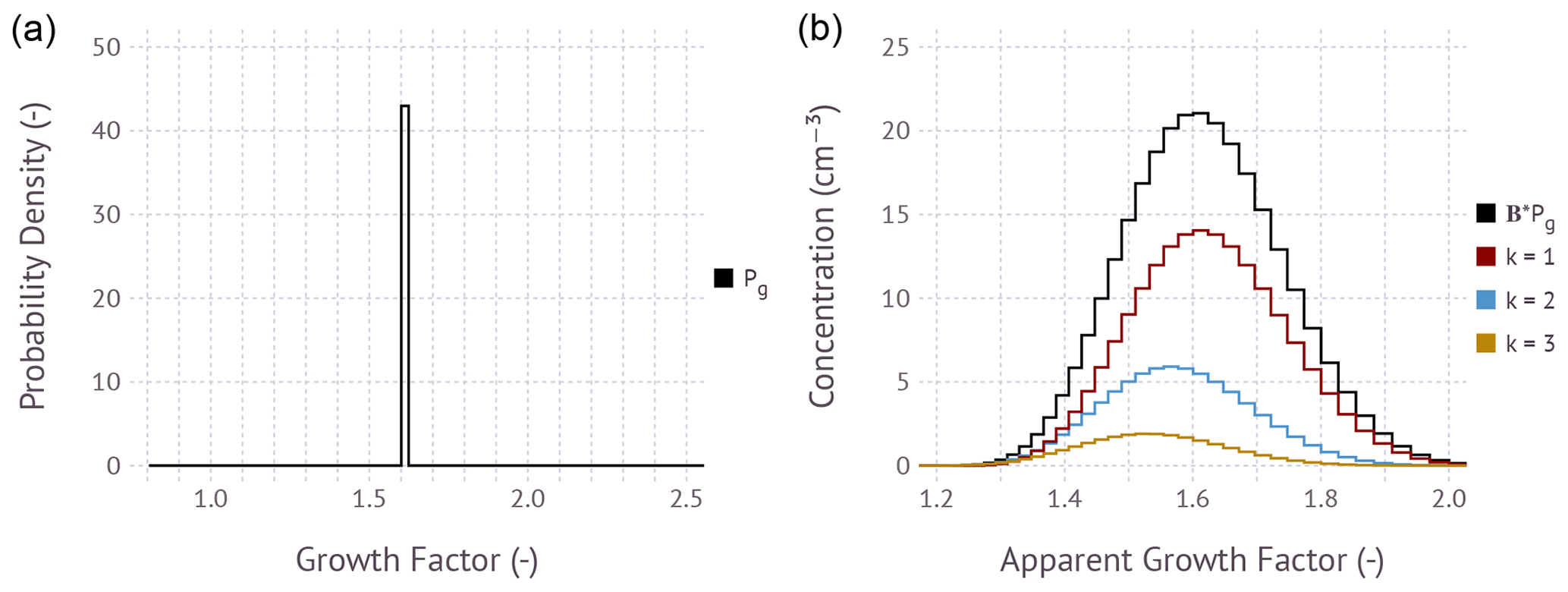
Figure 1(a) Input growth factor probability density $\mathrm{d}F/\mathrm{d}g$ assuming that all particles have a single growth factor of ∼ 1.6. The area under the curve evaluates to unity. (b) Modeled apparent mobility distribution function calculated using Eq. (15) and partial distributions for individual charges of k equals +1, +2, and +3 computed via ${\mathbf{O}}_{\text{k}}\cdot {\mathbb{M}}_{\text{k}}^{{\mathit{\delta }}_{\mathrm{1}}}$. The example is free of measurement error; i.e., ϵ=0. The black trace is what would be observed by a hypothetical measurement with a condensation particle counter.

Download

Figure 1 shows an example application of Eq. (18) for an input growth factor frequency distribution where all particles are assumed to have the same growth factor of ∼ 1.6. The frequency distribution is evaluated along a discrete growth factor grid with 120 bins with the range $\mathrm{0.8}<\mathit{g}<\mathrm{5}$. Note that the size grid (or apparent growth factor grid) must be extended to large sizes to capture the growth of multiply charged particles computed via Eq. (13). The assumed input size distribution is bimodal with mode diameters of 60 and 140 nm, geometric standard deviations of 1.4 and 1.6, and number concentrations of 1300 and 2000 cm⁻³ in modes 1 and 2, respectively. The assumed sheath-to-sample flow ratios are 5:1 in both DMAs. The product BP_g is the raw response that would be measured by a condensation particle counter at the exit of the instrument. The contribution of +1, +2, and +3 charged particles to the total can be computed via ${\mathbf{O}}_{\text{k}}\cdot {\mathbb{M}}_{\text{k}}^{{\mathit{\delta }}_{\mathrm{1}}}$. Although the nominal growth factor is the same for all sizes, the apparent mode of the growth factor decreases with increasing particle charge (see also Gysel et al., 2009; Shen et al., 2021). Therefore the axis is denoted as the apparent growth factor. Summing the partial distributions results in BP_g, demonstrating that the matrix equation correctly maps P_g to the response, including multiply charged particles.

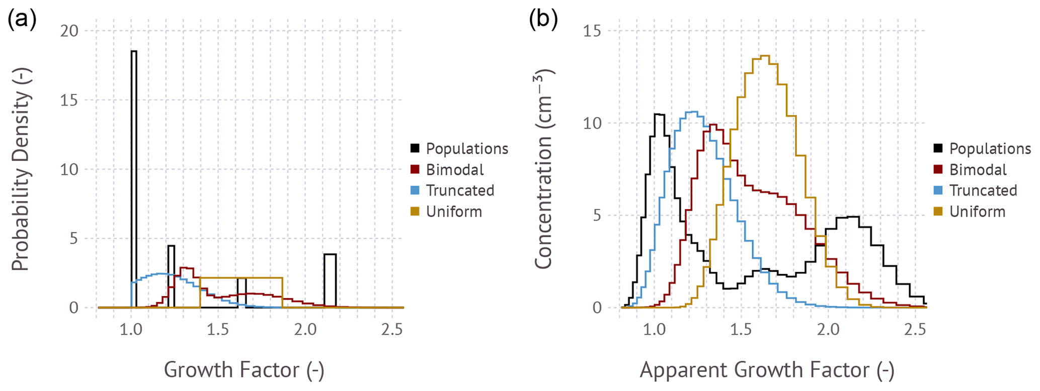
Figure 2(a) Illustrative input growth factor probability density distributions. The area under the curve evaluates to unity. (b) Corresponding modeled apparent mobility distribution function calculated using Eq. (15). The example is free of measurement error; i.e., ϵ=0.

Download

Figure 2 shows the relationship between four illustrative growth factor frequency distributions and the modeled apparent mobility distribution functions. The apparent mobility distribution function represents the raw particle concentration that would be measured by a detector as a function of the apparent + 1 mobility diameter. The diameter axis is normalized by the dry diameter selected by DMA 1. The selected examples comprise a testbed to evaluate the feasibility of an SMPS-style matrix-based inversion to recover P_g. The Populations example consists of an external mixture with compositions corresponding to four unique growth factors. The Bimodal example is the superposition of two Gaussian distributions with 70 % of particles in the less hygroscopic mode. The Truncated example is a Gaussian distribution truncated at g=1.0. The Uniform example is a uniform distribution over a fixed interval. All frequency distributions integrate to unity, thus accounting for 100 % of the particle population. The dry diameter and assumed input size distribution to compute the matrix B are the same as in Fig. 1. However, unlike in Fig. 1, the frequency distribution and matrix are evaluated along a coarser discrete growth factor grid with 60 bins with the range $\mathrm{0.8}<\mathit{g}<\mathrm{5}$. Note that the growth factor bin width is not constant, with wider bins at larger growth factors. This is due to the evaluation of the humidified size distribution along a geometrically stepped mobility grid. As will be shown next, 60-bin resolution is a suitable compromise between speed, accuracy, and resolution when computing the matrix-based inversion to infer P_g from noise-perturbed apparent growth factor frequency distributions.

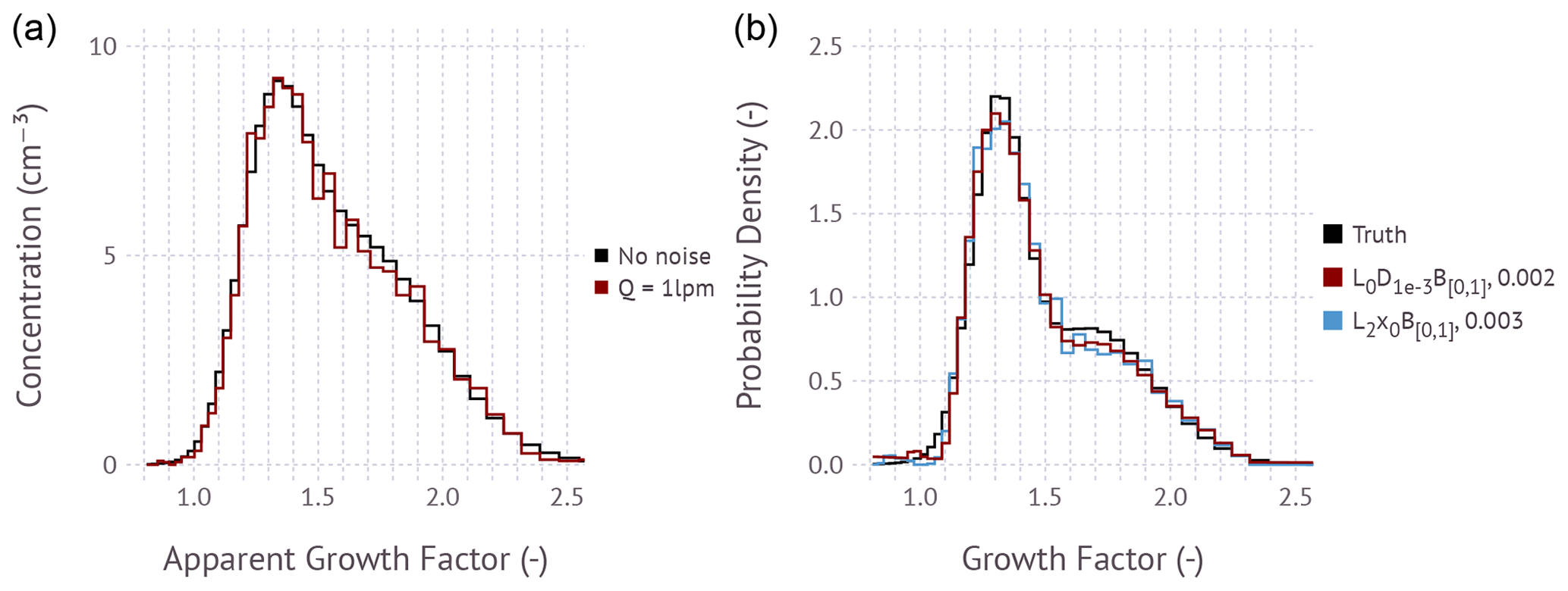
Figure 3(a) Humidified apparent growth factor distribution function for the Bimodal example comprising superposition of two Gaussian distributions with 70 % of particles in the less hygroscopic mode. The distributions are calculated as ${\mathbb{m}}_{\text{t}}^{{\mathit{\delta }}_{\mathrm{2}}}=\mathbf{B}{\mathit{P}}_{\text{g}}+\mathit{ϵ}$. “No noise” corresponds to ϵ=0. “Q=1 lpm” corresponds to the simulated Poisson noise equivalent for a condensation particle counter measuring at a flow rate of 1 L min⁻¹ and bin integration time of 2 s per bin. (b) Inverted growth factor probability density distribution using the $L_{\mathrm{0}}{D}_{\mathrm{1}e-\mathrm{3}}{B}_{[\mathrm{0},\mathrm{1}]}$ and L₂x₀B_[0,1] method. The area under the curve evaluates to unity. The a priori estimate x₀ is the normalized apparent growth factor distribution. Values in the legend (0.002 and 0.003) correspond to the root mean square error between the true input (Truth) and the regularized solution evaluated in frequency space.

Download

4.1 Data sources

4.1.1 Bodega Marine Laboratory

Aerosol size distribution data to contrast inversion schemes were obtained from measurements taken at Bodega Marine Laboratory (39^∘18^′25^′′ N, 123^∘3^′58^′′ W) between 16 January and 8 March 2015 as part of the CalWater 2/ACAPEX campaign. A subset of the data have been published by Atwood et al. (2019). Sample flow was brought into a mobile laboratory using an inlet, dried to 10±2 % relative humidity using a Nafion membrane drier, and brought to charge equilibrium using an X-ray source (TSI 3088, TSI Inc., Shoreview, MN, USA) prior to entering a cylindrical DMA column (TSI 3081). The DMA was configured to measure the size distribution in scanning mobility particle sizer mode. Voltage was scanned exponentially from 10 kV to 10 V over 300 s. A condensation particle counter (TSI 3771, flow rate 1 L min⁻¹) and a cloud condensation nuclei counter (DMT Model 100, Droplet Measurement Technologies, Boulder, CO, USA, flow rate 0.3 L min⁻¹) were used to measure particle concentration downstream of the DMA. The sheath-to-sample flow rate in the DMA was 5:1.3 L min⁻¹. Raw DMA response distributions comprising concentration measured by a condensation particle counter (CPC) vs. apparent + 1 mobility diameter were constructed along a 120-bin, geometrically stepped mobility grid. Response distributions are denoted as 𝕣. The apparent + 1 mobility diameter is computed from the centroid mobility selected by the DMA assuming that all particles are singly charged. The dynamic diameter range for this setup is from 12 to 550 nm. The inversion matrix A is computed using Eq. (11) for the diffusionally broadened transfer function (Stolzenburg and McMurry, 2008) and transmission loss correction through the DMA (Reineking and Porstendörfer, 1986). Inclusion of these terms results in a more ill-posed inverse problem due to increasing overlap between the kernels (Kandlikar and Ramachandran, 1999). The DMA response functions were inverted using the L₀x₀B_[0,∞] and L₂B_[0,∞] methods. The a priori estimate for L₀x₀B_[0,∞] was taken to be ${\mathit{x}}_{\mathrm{0}}={\mathbf{S}}^{-\mathbf{1}}\mathbb{r}$, where S is obtained by summing the rows of A and placing the results on the diagonal of S (Talukdar and Swihart, 2003). The method L₀x₀B_[0,∞] with ${\mathit{x}}_{\mathrm{0}}={\mathbf{S}}^{-\mathbf{1}}\mathbb{r}$ is essentially equivalent to the method used by Petters (2018), where it was shown that the thus-inverted spectra are similar to those output by the inversion algorithm employed by the commercial TSI Aerosol Instrument Manager software suite. Small differences between L₀x₀B_[0,∞] employed here and the approach of Petters (2018) include the use of generalized cross-validation instead of the L-curve method to search for the optimal regularization parameter and the method to eliminate negative values after inversion. Petters (2018) truncated negative values instead of using a least-squares numerical solver as described in Sect. 2.1.3.

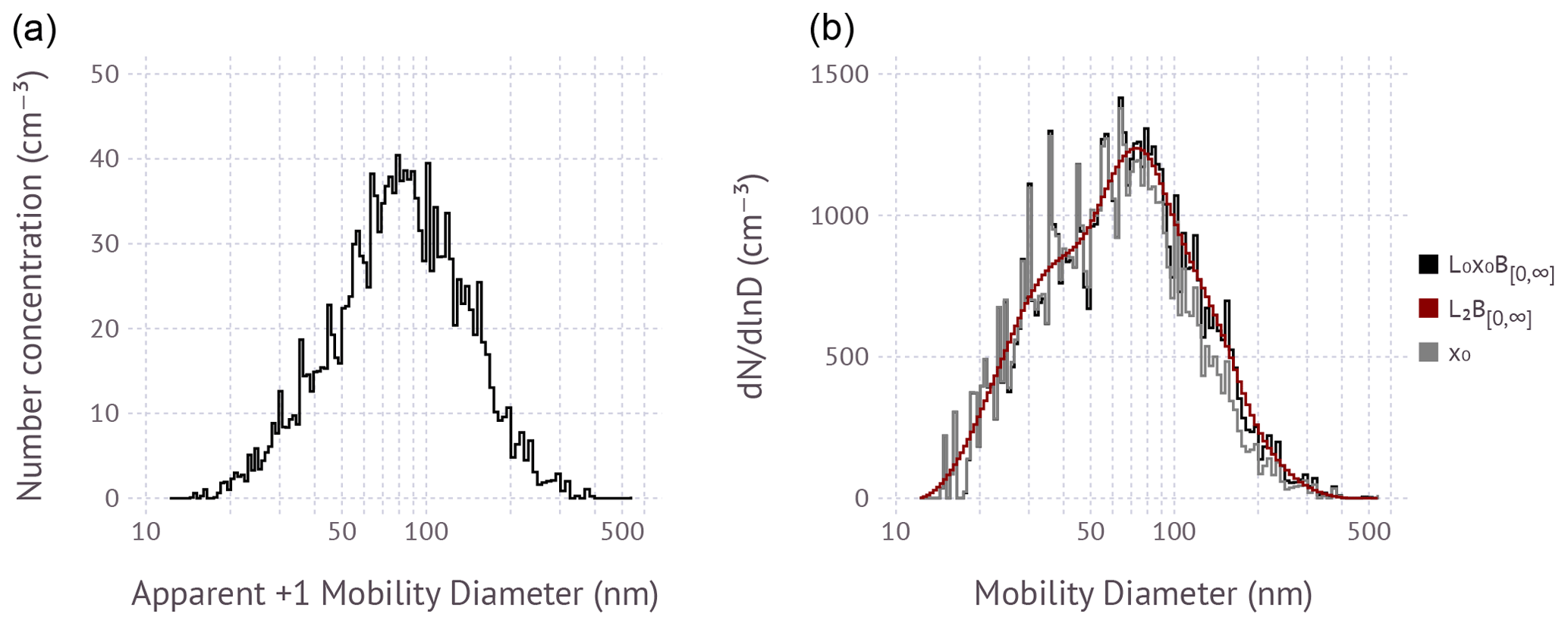
Figure 5(a) Raw DMA response function for a single scan on 5 March 2015 at 10:40 UTC at Bodega Marine Laboratory. (b) Inverted size distribution using the L₀x₀B_[0,∞] and L₂B_[0,∞] method and the a priori estimate of the solution ${\mathit{x}}_{\mathrm{0}}={\mathbf{S}}^{-\mathbf{1}}\mathbb{r}$.

Download

4.2 Results

4.2.1 Inversion of size distribution data (Bodega Marine Laboratory site)

Figure 5 shows a real-world example size distribution response function gridded into 120 size bins. The total particle concentration is ∼2000 cm⁻³. The ragged structure is typically explained by random noise due to Poisson counting statistics. However, in this example the noise level is larger than Poisson counting statistics alone, which is thought to be due to the processing of raw data internal to the specific CPC model that was used to collect the data. At this diameter resolution and with inclusion of the diffusion and loss terms in the forward model, the unregularized matrix inverse is entirely dominated by amplified random noise and is useless. The L₀x₀B_[0,∞] method converges to the solution with slight amplification of the random noise presented in the raw response function. The random noise is carried over into the a priori estimate ${\mathit{x}}_{\mathrm{0}}={\mathbf{S}}^{-\mathbf{1}}\mathbb{r}$, which roughly represents the noise visible in the reconstructed solution. Nevertheless, L₀x₀B_[0,∞] is highly robust and unlikely to go astray because x₀ is an excellent approximation of the solution at diameters of less than 100 nm where singly charged particles dominate and is a good initial estimate for larger particles. Second-order inversion using L₂B_[0,∞] produces a smooth, denoised solution due to application of the derivative operator in the regularization filter matrix. The solution converges even though no a priori estimate is used; i.e., x₀=0. Inclusion of an a priori in the form of L₂x₀B_[0,∞] is possible. However, noise in the a priori propagates into the solution, thus negating the intended benefit of the second-order Tikhonov matrix. The algorithms specified in Sect. 2.1.2 significantly speed up the inversion relative to previous versions of the software (Petters, 2018). Wall-clock times on an i7-8559U CPU for the inversion of a single spectrum are 5 and 2 ms for L₀x₀B_[0,∞] and L₂B_[0,∞], respectively. This contrasts to the 500 to 1000 ms required by the brute-force algorithm – approximately equivalent to L₀x₀B_[0,∞] – used previously. Finding the global minimum of V(λ) to identify the optimal regularization parameter also eliminates the occasional failure to converge when the L-curve algorithm is used (Petters, 2018). Either L₀x₀B_[0,∞] or L₂B_[0,∞], combined with generalized cross-validation, is suitable for use in routine unsupervised inversion of size distribution data.

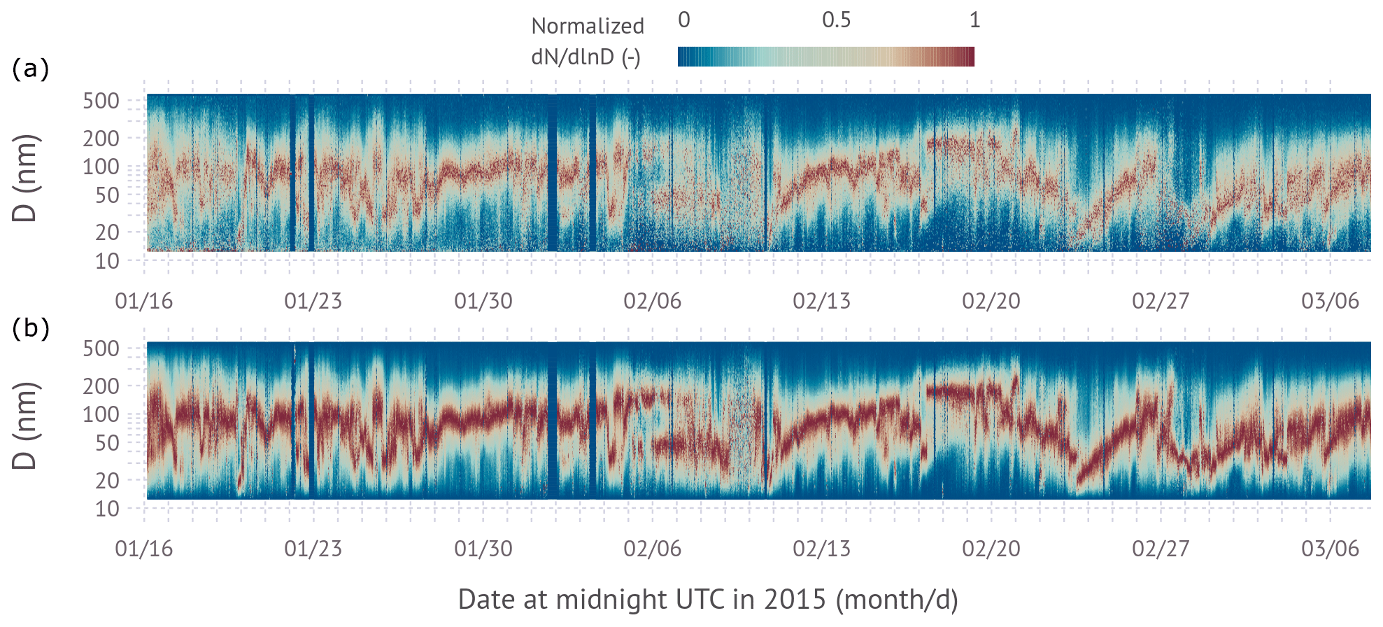
Figure 6Time evolution of the normalized particle size distributions collected between 16 January and 7 March at Bodega Marine Laboratory. The normalization is for each size distribution such that the maximum of the spectral density equals unity. The red color visualizes the time evolution of the mode diameter of the dominant mode. Top panel: inverted using L₀x₀B_[0,∞]; bottom panel: inverted using L₂B_[0,∞].

Download

Figure 6 shows the time evolution of the normalized particle size distributions over a 7-week period. The normalization is to highlight changes in the mode diameter(s). In general, the aerosol at the site is dominated by continental rural background conditions and the land–sea breeze circulation (Atwood et al., 2019). The time series is punctuated by aerosol transported from the California Central Valley to the site through the Petaluma Gap (Martin et al., 2017). Periods of low particle concentration occurred during the passage of an atmospheric river on 7–9 February 2015 and a marine inflow event on 27–28 February 2015. The atmospheric river brought heavy precipitation and marine air masses from the southwest direction, while the marine inflow event brought strong winds and precipitation-free maritime air from the northwest direction. Several periods of prolonged modal growth were observed starting, e.g., 11 and 24 February and 1 March 2015. Figure 6 demonstrates the influence of inversion noise on visualizing the dynamic evolution of the size distribution. The denoised L₂B_[0,∞] solution significantly improves visualization of modes without the need to reduce the size resolution in the inversion. The signal is especially improved during low-concentration periods during the atmospheric river passage and marine inflow event.

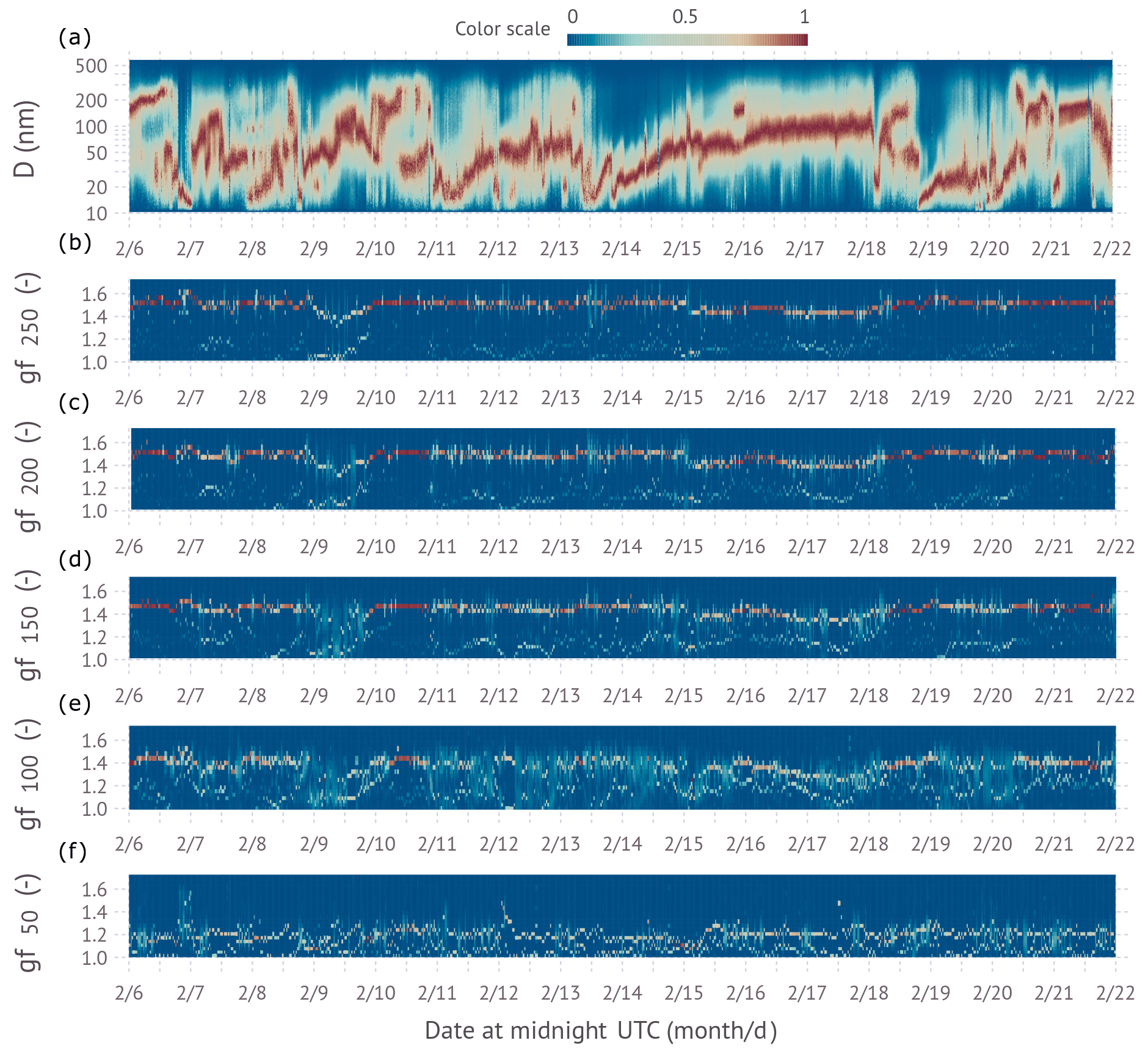
Figure 7(a) Time evolution of the normalized particle size distributions collected between 6 and 22 February at the Southern Great Plains research site. The normalization is for each size distribution such that the maximum of the spectral density equals unity. (b–f) Inverted growth factor frequency distributions at 85 % relative humidity for 250, 200, 150, 100, and 50 nm particles, respectively.

Download