the Creative Commons Attribution 4.0 License.
the Creative Commons Attribution 4.0 License.
 | 15 Oct 2021
Differential absorption lidar for water vapor isotopologues in the 1.98 µm spectral region: sensitivity analysis with respect to regional atmospheric variability
Jonas Hamperl
Clément Capitaine
Jean-Baptiste Dherbecourt
Myriam Raybaut
Patrick Chazette
Julien Totems
Bruno Grouiez
Laurence Régalia
Rosa Santagata
Corinne Evesque
Jean-Michel Melkonian
Antoine Godard
Andrew Seidl
Harald Sodemann
Cyrille Flamant
Laser active remote sensing of tropospheric water vapor is a promising technology to complement passive observational means in order to enhance our understanding of processes governing the global hydrological cycle. In such a context, we investigate the potential of monitoring both water vapor and its isotopologue HD16O using a differential absorption lidar (DIAL) allowing for ground-based remote measurements at high spatio-temporal resolution (150 m and 10 min) in the lower troposphere. This paper presents a sensitivity analysis and an error budget for a DIAL system under development which will operate in the 2 µm spectral region. Using a performance simulator, the sensitivity of the DIAL-retrieved mixing ratios to instrument-specific and environmental parameters is investigated. This numerical study uses different atmospheric conditions ranging from tropical to polar latitudes with realistic aerosol loads. Our simulations show that the measurement of the main isotopologue is possible over the first 1.5 km of atmosphere with a relative precision in the water vapor mixing ratio of <1 % in a mid-latitude or tropical environment. For the measurement of HD16O mixing ratios under the same conditions, relative precision is found to be slightly lower but still sufficient for the retrieval of range-resolved isotopic ratios with precisions in δD of a few per mil. We also show that expected precisions vary by an order of magnitude between tropical and polar conditions, the latter giving rise to poorer sensitivity due to low water vapor content and low aerosol load. Such values have been obtained for a commercial InGaAs PIN photodiode, as well as for temporal and line-of-sight resolutions of 10 min and 150 m, respectively. Additionally, using vertical isotopologue profiles derived from a previous field campaign, precision estimates for the HD16O isotopic abundance are provided for that specific case.


In many important aspects, climate and weather depend on the distribution of water vapor in the atmosphere. Water vapor leads to the largest climate change feedback, as it more than doubles the surface warming from atmospheric carbon dioxide (Stevens et al., 2009). Knowing exactly how water vapor is distributed in the vertical is of paramount importance for understanding the lower tropospheric circulation, deep convection, the distribution of radiative heating, and surface fluxes' magnitude and patterns, among other processes. Conventional radio-sounding or passive remote sensors, such as microwave radiometers or infrared spectrometers, are well-established tools used for water vapor profile retrieval in the atmosphere. However, apart from balloon-borne soundings, most of these instruments do not allow for determining how water vapor is distributed along the vertical in the 0–3 km above the surface which contains 80 % of the water vapor amount of the atmosphere. Additionally, passive remote sensors will generally require ancillary measurements such as aerosols, temperature or cloud heights to limit the errors in retrieved concentrations from radiance measurements. To complement these methods, active remote sensing techniques are expected to provide higher-resolution measurement capabilities especially in the vertical direction where the different layers of the atmosphere are directly probed with a laser. Among these active remote sensing techniques, Raman lidar is a powerful way to probe the atmosphere as it can give access to several atmospheric state parameters such as temperature, aerosols and the water vapor mixing ratio (WVMR) within a single line of sight (Whiteman et al., 1992). Benefiting from widely commercially available high-energy visible or UV lasers, as well as highly sensitive detectors, it allows high-accuracy, long-range measurements despite the small Raman scattering cross-section. WVMR retrieval from Raman lidar signals is however typically limited by parasitic daytime sky radiance and requires instrument constant and overlap function calibration (Whiteman et al., 1992; Wandiger and Raman, 2005). Conversely, the differential absorption lidar (DIAL) technique is in principle calibration-free since the targeted molecule mixing ratio can be directly retrieved from the attenuation of the lidar signals at two different wavelengths, knowing the specific differential absorption cross-section of the targeted molecule (Bösenberg, 2005). However, this benefit must be balanced with higher instrumental constraints especially on the laser source which is required to provide high power as well as high-frequency agility and stability at the same time. For water vapor this method has been successfully demonstrated essentially using pulsed laser sources emitting in the visible or near infrared (Bruneau et al., 2001; Wirth et al., 2009; Wagner and Plusquellic, 2018), and recent progress in the fabrication and integration of tapered semiconductor optical amplifiers has enabled the development of small-footprint field-deployable instrumentation (Spuler et al., 2015). The infrared region between 1.5 and 2.0 µm has also attracted interest for water vapor DIAL sounding, especially in the context of co-located methane and carbon dioxide monitoring (Wagner and Plusquellic, 2018; Cadiou et al., 2016). One of the potential benefits of co-located multiple-species measurement would be to reduce the uncertainties related to the retrieval of dry-air volume mixing ratios for the greenhouse gas (GHG) of interest. This aspect has particularly been studied in the field of space-borne integrated path differential absorption (IPDA) lidar for carbon dioxide (CO2) monitoring in the 2.05 µm region where water vapor absorption lines may affect the measurement (Refaat et al., 2015). One great potential of these multiple-wavelengths and multiple-species approaches would be their adaptability to isotopologue measurements with the DIAL technique since isotopic ratio estimation is equivalent to multiple-species measurement provided the targeted isotopologues display similarly suitable and well-separated absorption lines in a sufficiently narrow spectral window.
Humidity observations alone are not sufficient for identifying the variety of processes accounting for the proportions and history of tropospheric air masses (Galewsky et al., 2016). Stable water isotopologues, mainly , HD16O and differ by their mass and molecular symmetry. As a result, during water phase transitions, they have slightly different behaviors. The heavier molecules prefer to stay in the liquid or solid phase while the lighter ones tend to evaporate more easily, or prefer to stay in the vapor phase. This unique characteristic makes water isotopologues the ideal tracers for processes in the global hydrological cycle. Water isotopologues are independent quantities depending on many climate factors, such as vapor source, atmospheric circulation, precipitation and droplet evaporation, and ambient temperature. So far, no lidar system has been investigated for the measurement of water vapor isotopologues other than (hereafter referred to as H2O). Here, in the framework of the Water Vapor Isotope Lidar (WaVIL) project, we investigate the possibility of using a transportable differential absorption lidar to measure the concentration of both water vapor H2O and the isotopologue HD16O (hereafter referred to as HDO) at high spatio-temporal resolutions in the lower troposphere (Hamperl et al., 2020). The proposed lidar will operate in the 2 µm spectral region where water vapor isotopologues display close but distinct absorption lines. Such an innovative remote sensing instrument would allow the monitoring of water vapor and HDO isotopic abundance profiles with a single setup for the first time, enabling the improvement of knowledge of the water cycle at scales relevant for meteorological and climate studies.
The purpose of this paper is to assess the expected performances of a DIAL instrument for probing of H2O and HDO in the lower troposphere. In Sect. 2, the choice of the sensing spectral range is substantiated and the performance model is outlined. The approach for modeling transmitter, detection and environmental parameters is detailed. The sensitivity analysis is based on representative average columns of arctic, mid-latitude and tropic environments. The simulation results and an extensive error analysis are presented in Sect. 3. To assess the random uncertainty in the retrieved isotopologue mixing ratio, major detection noise contributions are analyzed for a commercial InGaAs PIN and a state-of-the-art HgCdTe avalanche photodiode. Instrument- and atmosphere-specific systematic errors are discussed for different model environments. Finally, performance calculations are applied to vertical profiles retrieved from a past experimental campaign where a Raman lidar for water vapor measurements and in situ sensors for the HDO isotopologue measurements were deployed. A conclusion and perspectives for forthcoming calibration and validation field campaigns are given in Sect. 4.
2.1 Choice of the sensing spectral range
Remote sensing by DIAL relies on the alternate emission of at least two closely spaced laser wavelengths, one coinciding with an absorption line of the molecule of interest (λon) and the other tuned to the wing of the absorption line (λoff), to retrieve a given species concentration. The key to independently measuring HDO and H2O abundances with a single instrument lies thus in the proper selection of a spectral region where (i) the two molecules display well-separated, significant absorption lines while minimizing the interference from other atmospheric species and (ii) the selected lines preserve a relatively equal lidar signal dynamic and relative precision ranges for both isotopologues. This makes the line selection rather limited. Using spectroscopic data from the HITRAN2016 database (Gordon et al., 2017), we investigated the possibilities for HDO sounding at up to 4 µm, where robust pulsed nanosecond lasers or optical parametric oscillator sources based on mature lasers or nonlinear crystal components can be developed (Godard, 2007). Figure 1a shows that HDO lines are strong in the 2.7 µm region but overlap with an even more dominant H2O absorption band. Considering the state of possible commercial photodetector technologies, we chose to limit the range of investigation to 2.6 µm, corresponding to the possibilities offered by InGaAs photodiodes. In the telecom wavelength range, which offers both mature laser sources and photodetectors, HDO absorption lines are too weak to be exploited for DIAL measurements over 1–3 km. The same argumentation holds for wavelengths towards 2.05 µm (see Fig. 1b) which have been extensively studied for space-borne CO2 IPDA lidar sensing (Singh et al., 2017; Ehret et al., 2008). However, the 2 µm region seems to offer an interesting possibility in terms of absorption strength as well as technical feasibility of pulsed, high-energy, single-frequency laser sources (Geng et al., 2014). The spectral window between 1982–1985 nm is well suited to meeting the mentioned requirements as illustrated in Fig. 1c. In this paper we will focus on the line at 5043.0475 cm−1 (1982.93 nm) and the HD16O lines at 5044.2277 cm−1 (1982.47 nm) and 5040.4937 cm−1 (1983.93 nm), hereafter referred to as HDO options 1 and 2, respectively, allowing for a sufficiently high absorption over several kilometers with negligible interference from other gas species. Additionally, a second option for H2O slightly detuned from the absorption peak at 1982.97 nm will be discussed as a possibility for reducing the temperature sensitivity of the DIAL measurement (hereafter referred to as H2O option 2). Wavelength switching will be realized on a shot-to-shot basis to consecutively address the chosen on-line wavelengths and the off-line wavelength at 1982.25 nm for H2O (1 and 2) and HDO (1) or the off-line wavelength at 1983.72 nm for HDO (2). As shown in Fig. 1c, the HDO absorption line at 1982.47 nm is accompanied by a non-negligible H2O absorption which has to be corrected for when retrieving the volume mixing ratio and thus adds a bias dependent on the accuracy of the H2O measurement at 1982.93 nm. Furthermore, the interfering H2O line has a ground-state energy of 2756 cm−1 (see Table 1) which makes it highly temperature sensitive. Probing HDO at 1982.47 nm thus requires highly accurate knowledge of the H2O and temperature profile through auxiliary measurements (lidar, radio sounding). The alternative second option for HDO at 1983.93 nm avoids any H2O interference; however with slightly weaker absorption optical depth it gives rise to smaller signal-to-noise ratios and consequently increased measurement statistical uncertainty.
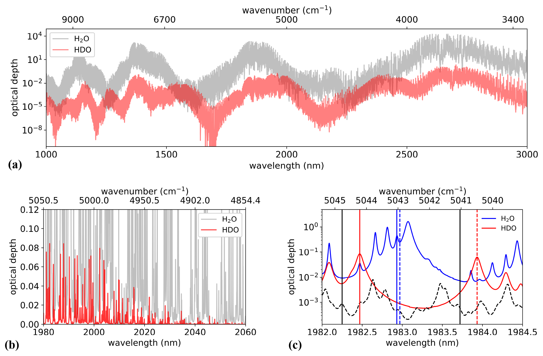
Figure 1Optical depth over 1 km for (H2O) and HD16O (HDO) with uniform volume mixing ratios of 8400 and 2.6 ppmv, respectively (relative humidity of 50 % at 15 ∘C). (a) Spectral overview between 1 and 3 µm. (b) Close-up window for wavelengths around 2 µm with decreasing HDO absorption towards 2.05 µm. (c) Spectral range of interest for simultaneous H2O and HDO sounding. The dashed black line represents the total optical depth of other species (CO2, CH4, N2O) with their typical atmospheric concentrations. Vertical black lines indicate the positions of possible off-line wavelengths. On-line wavelengths are indicated for H2O (vertical blue line for option 1 at 1982.93 nm, dashed blue line for option 2 at 1982.97 nm) and HDO (vertical red line for option 1 at 1982.47 nm, dashed red line for option 2 at 1983.93 nm). Spectra calculations are based on the HITRAN2016 database assuming a temperature of 15 ∘C and an atmospheric pressure of 1013.25 hPa.
Table 1Spectroscopic parameters for selected absorption lines.
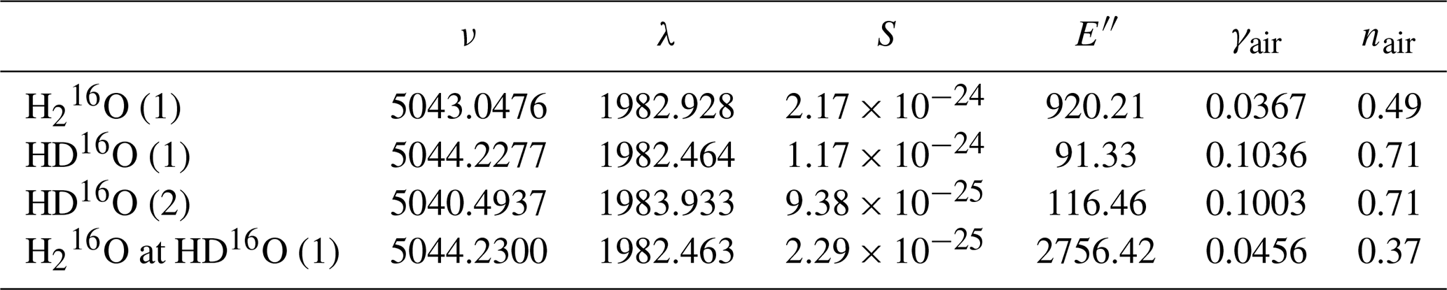
ν (cm−1): wavenumber; λ (nm): vacuum wavelength; S (): line intensity at 296 K; E′′ (cm−1): lower-state energy; γair (): air-broadened Lorentzian half width at half maximum (HWHM) at 1 atm and 296 K; nair: temperature exponent for γair.
In any of the proposed cases, addressing the on-line and off-line spectral features requires a tuning capability larger than 0.5 nm, which can be offered, for instance, by an optical parametric oscillator source (Cadiou et al., 2016; Barrientos Barria et al., 2014), which is envisioned for use with the WaVIL system. It should be noted that the chosen absorption lines do not fulfill the criterion of temperature insensitivity as outlined by Browell et al. (1991) which imposes the strict knowledge of the temperature profile along the lidar line of sight from auxiliary measurements for an accurate isotopologue retrieval.
2.2 DIAL performance model
The objective of the presented performance model is to elaborate the precision achievable with the proposed DIAL instrument of the volume mixing ratios of the water isotopologues H2O and HDO and thus of the precision on the measurement of HDO abundance (noted δD) which expresses the excess (or defect) of the deuterated isotope compared to a reference value of (1 HDO molecule for 3115 H2O molecules) (Craig, 1961). Following the convention, the HDO abundance (in per mil, ‰) is expressed as the deviation from that of the standard mean ocean water (SMOW) in the so-called notation:
where [ ] represents the concentration of H2O and HDO.
As schematically depicted in Fig. 2, the DIAL simulator consists of three sub-models describing atmospheric properties, lidar instrument parameters and detector properties. Each model will be explained in more detail in the following paragraphs. The atmosphere model is based on a set of standard profiles of temperature, pressure and humidity representative of different climate regions along with aerosol optical depth data of the AERONET database (https://aeronet.gsfc.nasa.gov/, last access: 2 October 2021). Those data are exploited to calculate the atmospheric transmission using absorption cross-sections computed with the HITRAN2016 spectroscopic database (Gordon et al., 2017). Together with the model describing the lidar instrument, the calculated transmission data are used to feed the lidar equation in order to calculate the received power at each selected on-line and off-line wavelength. In a subsequent step, noise contributions arising from the detection unit are taken into account to estimate the signal-to-noise ratio. Then, we use an analytical approach based on an error propagation calculation to estimate the random error in the measured isotopic mixing ratios and thus the uncertainty in the δD retrieval obtained with the simulated instrumental parameters.
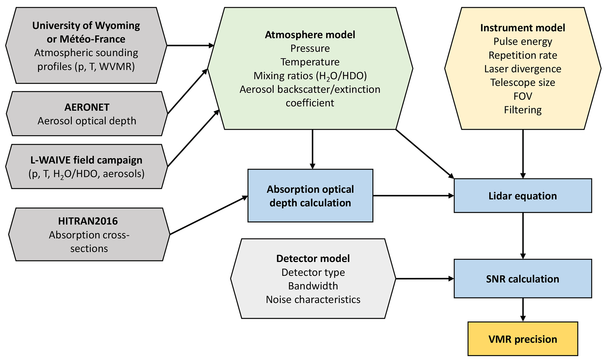
Figure 2Block diagram of the DIAL simulator. Input models and databases are in hexagons, and principal calculations are indicated by rectangles. p: pressure; T: temperature; WVMR: water vapor mixing ratio; FOV: telescope field of view. The signal-to-noise ratio (SNR) is used to calculate the statistical random error (precision) of the volume mixing ratio (VMR) of .
Starting from the lidar equation (Collis and Russell, 1976), the calculated received power as a function of distance r is written as
where Tr is the receiver transmission (assumed value of 0.5 for all calculations), A is the effective area of the receiving telescope, βπ(r) is the backscatter coefficient, O(r) is the overlap function between the laser beam and the field of view of the receiving telescope, c is the speed of light, Tatm(r) is the one-way atmospheric transmission, and Ep is the laser pulse energy. The DIAL technique is based on the emission of two wavelengths, one at or close to the peak of an absorption line (λon) and another tuned to the absorption line's wing (λoff).
Provided that the two laser pulses are emitted sufficiently close in wavelength and in time for the atmospheric aerosol content to be equivalent, they experience the same backscattering along the line of sight, and the differential optical depth Δτ as the difference in on- and off-line optical depth at a measurement range r can be retrieved by
with Pon and Poff as the backscattered power signals for λon and λoff, respectively. Using the optical depth measurement, the gas concentration can be retrieved at a remote range r within a range cell . Assuming Δr is sufficiently small, the water vapor content expressed as the volume mixing ratio, which is assumed as constant within Δr, can then be derived by
with WF(r) representing a weighting function defined as
where ρair is the total air number density and σon and σoff are the on-line and off-line absorption cross-sections calculated with the HITRAN2016 spectroscopic database assuming a Voigt profile representation of the form
with
where S is the line strength, γD is the Doppler width, γ is the pressure-broadened linewidth and ν0 is the line center position. The temperature T dependence of the line strength is determined by the energy of the lower molecular state E′′ according to
where T0 is the reference temperature, k is the Boltzmann constant and c is the speed of light.
Equation (3) is valid for the detection of the main isotopologue H2O. For HDO however, the presence of H2O absorption at the on-line wavelength of HDO (see Fig. 1c) necessitates an additional consideration of that bias for the inversion. Taking this into account, Eq. (3) changes to
where represents the H2O differential optical depth at the HDO on-line wavelength λHDO, which can be calculated with the knowledge of the volume mixing ratio measured at .
To obtain an analytical expression for the random error in the concentration measurement, an error propagation calculation can be applied to Eqs. (3) and (4) assuming that the range cell interval Δr is sufficiently small and that the range cell resolution of the receiver is sufficiently high to consider Δτ(r1) and Δτ(r2) uncorrelated. The absolute uncertainty in the volume mixing ratio X expressed as the standard deviation σ(X) can be calculated from the signal-to-noise ratios of the on- and off-line power signals as follows:
where Δf is the measurement bandwidth which is the same for the on- and off-line pulses since they are measured sequentially by the same detector. Finally, with both uncertainties in the volume mixing ratios and XHDO known, an estimation of the uncertainty in δD is obtained by applying an error propagation calculation to Eq. (1) in order to obtain the expected uncertainty expressed as variance:
2.3 Instrument and detector model
In order to estimate the feasibility of a DIAL measurement, calculations were performed for the transmitter and receiver parameters summarized in Table 2. The emitter of the DIAL system will be based on a generic optical parametric oscillator–optical parametric amplifier (OPO–OPA) architecture like the one developed in Barrientos Barria et al. (2014). The combination of a doubly resonant nested-cavity OPO (NesCOPO) and an OPA pumped by a 1064 nm Nd:YAG commercial laser with a 150 Hz repetition rate allows for single-frequency, high-energy pulses with adequate tunability. From this system we expect an extracted signal energy of up to 20 mJ at 1983 nm. For a more conservative estimate, we will also consider a lower-limit pulse energy of 10 mJ for our simulations. The receiver part consists of a Cassegrain-type telescope with a primary mirror of 40 cm in diameter. For the detection part, calculations were performed in a direct-detection setup for (i) a commercial InGaAs PIN photodiode and (ii) a HgCdTe avalanche photodiode (APD) specifically developed for DIAL applications in the 2 µm range, presented in Gibert et al. (2018). The telescope field of view is determined by an aperture in the telescope's focal plane. For better comparability, we assume the same aperture diameter of 1.2 mm for both the PIN photodiode and the APD. Given the small active area of the APD, imaging of the field of view on the detector might, however, prove extremely challenging in practice. The measurement bandwidth of the DIAL system is effectively determined by an electronic low-pass filter in the detection chain. In the simulation we use a bandwidth setting of 1 MHz corresponding to a spatial resolution of the retrieved isotopologue concentrations of 150 m. For all our calculations we assume signal averaging over an integration time of 10 min (45 000 laser shots for the on- and off-line wavelength).

In order to quantify the measurement uncertainty in the retrieved isotope mixing ratios, random and systematic sources of errors are taken into account. Random errors in measuring the differential optical depth, and thus the species mixing ratio, are related to different noise contributions arising from the detection setups. For a single return-signal pulse, the associated noise power Pn consists of a constant detector and amplifier noise expressed as noise-equivalent power NEP, shot noise due to background radiation Psky, shot noise dependent on the pulse power P(λ) and speckle noise Psp(λ):
where e is the elementary charge, F the excess noise factor (in the case of the APD), R the detector responsivity (depending on quantum efficiency in the case of the APD) and Δf the measurement bandwidth. The NEP of 600 for configuration i featuring the InGaAs PIN photodiode is a conservative estimate by calculations based on the specifications of the photodiode and amplifier manufacturer (G12182-003K InGaAs PIN photodiode from Hamamatsu combined with a gain-adjustable DHPCA-100 current amplifier from FEMTO). The background power Psky depends on the background irradiance Ssky and the receiver geometry according to
where Δλf, Aeff and θFOV are the optical filter bandwidth, effective receiver telescope area and field of view angle, respectively. A constant background irradiance of 1 W m−2 µm−1 sr−1 and an optical filter bandwidth of 50 nm are used for all calculations. Assuming Gaussian beam characteristics, the speckle-related noise power is approximately given by Ehret et al. (2008):
where Rtel denotes the telescope radius and τc the coherence time of the laser pulse corresponding to the pulse duration for a Fourier-transform-limited pulse. Finally, the overall time-averaged signal-to-noise ratio is given as the ratio of received power from Eq. (2) and total noise power from Eq. (11) multiplied by the square root of the number of laser shots N:
2.4 Atmosphere model
We constructed different atmospheric models for mid-latitude, arctic and tropical locations to study the sensitivity of the DIAL measurement to environmental factors. The atmosphere model consists of vertical profiles of pressure, temperature and humidity (see Appendix A for origin of sounding data) which serve as input to calculate altitude-dependent absorption cross-sections using the HITRAN2016 spectroscopic database. For the sake of simplicity, HDO mixing ratios were obtained from H2O profiles simply by considering their natural abundance of ; i.e., variability in terms of the isotopic ratio δD is not assumed in our model. For each location, a baseline model was constructed by using the columns of pressure, temperature and volume mixing ratios averaged over the year of 2019. To reflect seasonal variations in our sensitivity analysis, we use profiles with the lowest and highest monthly averages of temperature and humidity (Fig. 3a–c). To complement the atmospheric model, data of level 2.0 aerosol optical depth (AOD) from the AERONET database (https://aeronet.gsfc.nasa.gov/, last access: 2 October 2021) were used. AERONET sun-photometer products are usually available for wavelengths between 340 and 1640 nm. For extrapolation to the 2 µm spectral region, we used the wavelength dependence of the AOD described by a power law of the form (Ångström, 1929)
where AOD(λ) is the optical depth at wavelength λ, AOD(λ0) is the optical depth at a reference wavelength and α represents the Ångström exponent. The Ångström exponent was obtained by fitting Eq. (15) to the available AOD data in the above-mentioned spectral range in order to extrapolate further to 1.98 µm. Histograms of the yearly distribution of the extrapolated AOD at 1.98 µm are shown in the right column of Fig. 3g–i. Median values of the AOD are used for the baseline model. The lowest (AOD10) and highest (AOD90) decile values serve as input for the sensitivity analysis to model conditions of low and high aerosol charge, respectively. As a next step, vertical profiles of aerosol extinction are constructed by making basic assumptions about their shape and constraining their values by the extrapolated AOD. In our baseline model, the vertical distribution of aerosols is represented by an altitude-dependent Gaussian profile of the extinction coefficient with varying half width depending on the location (Fig. 3d–f). This type of profile roughly corresponds to the ESA Aerosol Reference Model of the Atmosphere (ARMA) (ARMA, 1999) which is plotted for each region normalized to the AOD90-derived extinction profile maximum.
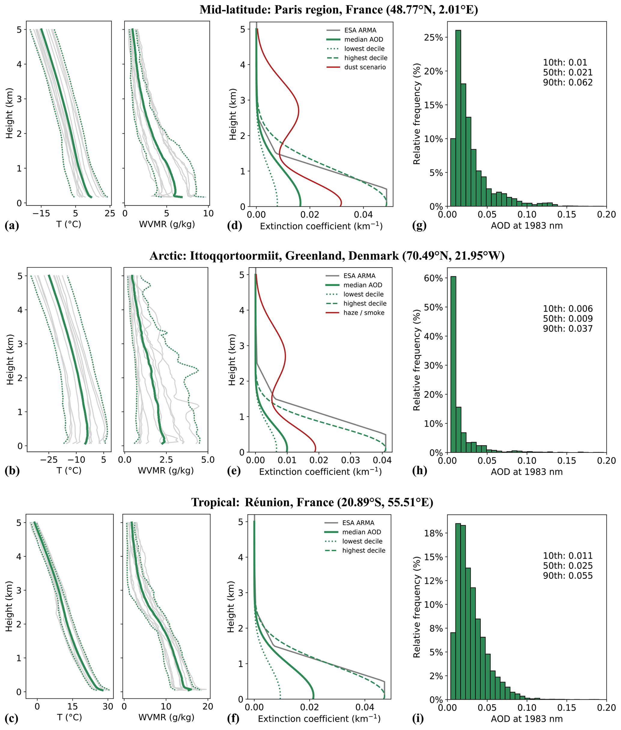
Figure 3Atmosphere models: (a–c) vertical sounding profiles of temperature and the water vapor mixing ratio (WVMR). Grey lines indicate monthly averages; solid green line is the yearly average of 2019 (baseline profile). Dotted lines indicate profiles of the lowest and highest monthly temperatures and WVMR; (d–f) model profiles of aerosol extinction coefficient; (g–i) distribution of the aerosol optical depth at 1983 nm for AERONET level 2.0 data of 2019.
However, the distribution of tropospheric aerosols varies widely from region to region (Winker et al., 2013). To broadly reflect the different boundary layer characteristics for each environment, the extinction profile was adapted accordingly. In mid-latitude regions, vertical aerosol distributions vary widely due to regional and seasonal factors (Chazette and Royer, 2017). The planetary boundary layer (PBL) height can range from a few hundred meters up to 3 km (Matthias et al., 2004; Chazette et al., 2017). Assuming that aerosols are mostly confined to the PBL and that the free tropospheric contribution to aerosol extinction is weak, the half-Gaussian-shaped baseline model used for the simulations gives rise to 85 % of AOD within the first 1.5 km. Since high aerosol loads in the free troposphere due to long-range dust transport are not uncommon over western Europe (Ansmann et al., 2003), a dust scenario profile constrained by the highest-decile AOD was also investigated. Dust aerosols are represented by a Gaussian profile above the PBL extending well up to a height of 5 km. For this case, aerosol extinction in the PBL below 1.5 km accounts for half of the total AOD, while dust in the free troposphere accounts for the other half. At high latitudes, the boundary layer tends to be stable and extends from a few meters to a few hundred meters above ground. Our baseline Arctic extinction profile thus contains 95 % of the AOD within the first 1.5 km since most aerosols are confined within the first kilometer of the troposphere as observed by space-borne lidar during long-term studies of the global aerosol distribution (Di Pierro et al.,2013). The occurrence histogram in Fig. 3h shows very low values of AOD for most of the time in the available photometer products from February to September. The long-tailed wing of the asymmetric distribution towards higher values can be explained by seasonally occurring episodes of arctic haze due to anthropogenic aerosols transported from mid-latitude regions (winter to spring) and boreal forest fire smoke during the summer season (Tomasi et al., 2015; Chazette et al., 2018).
Similarly to the dust scenario for the mid-latitude model, haze and smoke events are modeled by an additional Gaussian profile in the free troposphere constrained by the highest-decile AOD. Extinction profiles representing the tropical environment of the island of Réunion, where sea salt aerosols can be assumed to be the dominant aerosol species, are chosen such that 90 % of the AOD is attributed to the first 1.5 km.
Vertical profiles of the aerosol backscatter coefficient were calculated assuming, for the sake of simplicity, a constant extinction-to-backscatter ratio (lidar ratio) of 40 sr throughout all sets of extinction profiles.
3.1 Instrument random error
This section aims to quantify the random error in the mixing ratio measurement depending on instrument settings such as laser pulse energy and the type of detector employed. All calculations are based on the mid-latitude baseline atmosphere model assuming vertical sounding of the lower troposphere with aerosols confined to the lowest 2 km. Considering a simple calculation of random errors, we will discuss their implications for the precision of the measurement of range-resolved δD profiles. Given the instrument parameters presented in Table 2, the dominant noise contributions are estimated, which are shown for a single on-line pulse in Fig. 4 for both detector configurations.
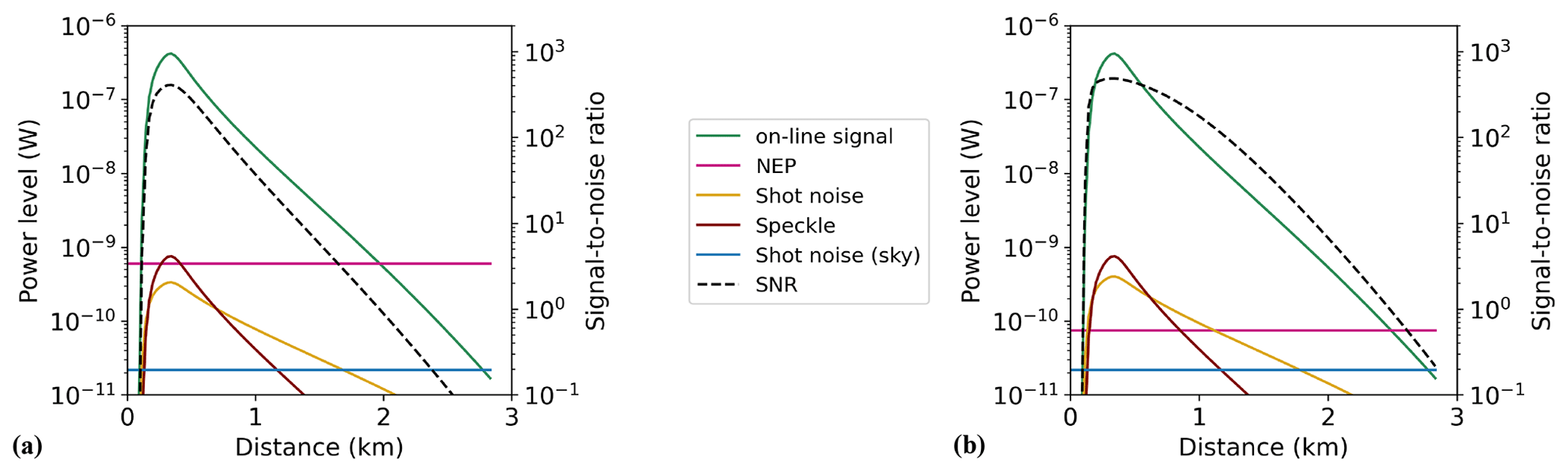
Figure 4Received power according to Eq. (2) (solid green line) and power-equivalent levels of major noise contributions related to the H2O on-line signal for a single 20 mJ pulse and resulting signal-to-noise ratio (SNR, dashed black line, right vertical axis) as function of lidar range: (a) InGaAs PIN detector, (b) low-noise HgCdTe APD.
As expected, the electronic noise level is significantly reduced by roughly 1 order of magnitude for the HgCdTe APD combined with a transimpedance amplifier due to a low combined NEP of 75 compared to 600 for the amplifier of the InGaAs PIN detector. In fact, shot noise and speckle are predominant for the APD for the first kilometer of range, whereas the electronic noise of the transimpedance amplifier is the predominant contribution over the entire range for the commercial PIN detector. Signal-to-noise ratios of up to 102 are obtained for a single measurement pulse within the first kilometer. Integrating over 45 000 laser shots (equivalent to 10 min averaging time if on- and one off-line wavelengths are addressed sequentially) would increase the signal-to-noise ratios to over 104 in the first kilometer for both detectors and to values around 102 at a 2 km range for the commercial PIN detector and 103 for the HgCdTe APD.
The expected relative random errors in the mixing ratios of H2O and HDO are shown separately for each detector in the upper and lower panels of Fig. 5. We examined two scenarios with different laser pulse energies of 10 and 20 mJ, a measurement bandwidth of 1 MHz (150 m range cell resolution), and an integrating time of 10 min for a repetition rate (on–off rate) of 150 Hz. The simulation based on the 20 mJ configuration gives an estimation of the best-case precision limit of the DIAL system. The second configuration with 10 mJ pulse energy can be understood as a lower limit on the precision of measuring mixing ratios of H2O and HDO and finally δD.
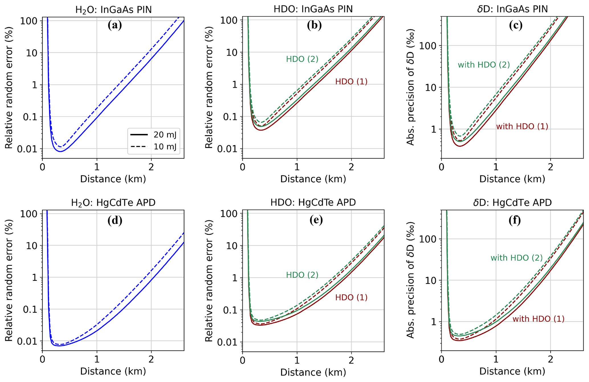
Figure 5Expected relative random error in the volume mixing ratio of H2O and HDO for different pulse energies (solid lines: 20 mJ; dashed lines: 10 mJ) and detectors: (a–b) InGaAs PIN detector, (d–e) HgCdTe APD. (c, f) Corresponding absolute uncertainty (standard deviation) in δD as a function of distance from the lidar instrument. A detection bandwidth of 1 MHz is assumed, and signal averaging time is 10 min.
As shown in Fig. 5, a relative random error of well under 1 % in the mixing ratio of both H2O and HDO can be achieved within the first kilometer for both detectors and 20 mJ pulse energy. The degraded precision for measuring HDO is due to its lower differential absorption compared to H2O. The slight difference in optical depth for the two HDO options leads only to a small loss in precision for wavelength option 2. For the low-noise APD shown in the bottom panel of Fig. 5, the simulations show that even for the conservative assumption of 10 mJ pulse energy, the relative error stays below 1 % for both H2O and HDO over a range of 1.5 km corresponding to typical heights of the planetary boundary layer. H2O uncertainties were calculated for sounding at the peak of the absorption line (option 1). The simulation results also reveal a sharp rise in the random uncertainty towards longer distances which is attributed to the drastic decline in aerosol backscatter in the free troposphere in our model. The sharp fall of the random error within the first 200–300 m is due to the increasing overlap between the laser beam and telescope field of view imaged onto the detector described by the overlap function O(r) in Eq. (2). This overlap term is zero directly in front of the lidar instrument and reaches unity after around 450 m for the here-described configuration. It should be noted that for the range zone of non-uniform overlap, slight differences between the on- and off-line overlap, for example due to laser beam pointing, can induce significant systematic errors. From a practical point of view, the expected lowest instrument range is thus closer to 0.5 km than the distance suggested by the location of the random error minima around 250 m.
Figure 5c and f show the expected precision in δD which depends on the relative random errors in the volume mixing ratios for H2O and HDO (see Eq. 9). For the commercial InGaAs PIN photodiode we find for the best-case configuration (20 mJ pulse energy, 1 MHz bandwidth) that the absolute value of uncertainty in δD is below 3 ‰ within a range of 1 km. The 10 mJ configuration also allows for measurement of δD, although with deteriorated absolute precision of up to 10 ‰ within the first kilometer. For greater ranges, the precision levels decline rapidly and are not sufficient to resolve variations in δD on the order of a few tens of per mil. The use of a HgCdTe APD detector can overcome this limitation where calculations indicate that an absolute precision level better than 10 ‰ within a range of close to 2 km can be achievable with 20 mJ laser energy.
3.2 Sensitivity to atmospheric variability
The sensitivity of the DIAL instrument to the variability in temperature, humidity and aerosol load was investigated for the mid-latitude, arctic and tropical atmosphere models. In the following analysis, the relative random error (precision) is used to compare the influence of each atmospheric parameter under investigation. Simulation results are summarized in Fig. 6 for targeting H2O at 1982.93 nm (blue) and HDO at 1983.93 nm (red). Here again, we consider a measurement bandwidth of 1 MHz (150 m range cell resolution) and an integrating time of 10 min for a repetition rate of 150 Hz. All calculations have been performed with the InGaAs PIN detector and assuming a laser pulse energy of 20 mJ.
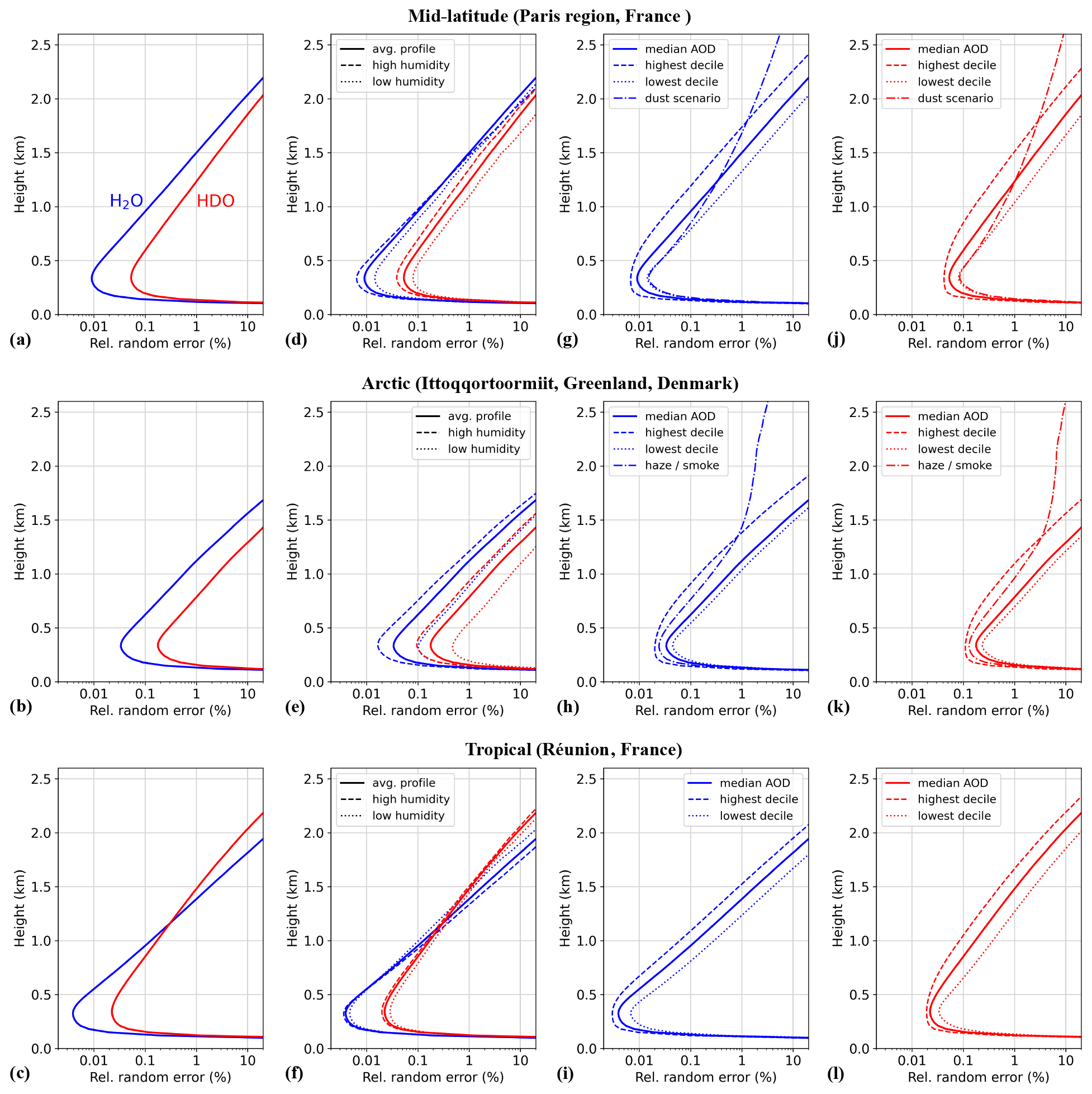
Figure 6Sensitivity with respect to variability in atmospheric parameters: resulting statistical uncertainty for range-resolved DIAL measurement of H2O (blue, option 1 at 1982.93 nm) and HDO (red, option 2 at 1983.93 nm). Simulation parameters: 20 mJ pulse energy, 1 MHz bandwidth, 10 min integration time, InGaAs PIN detector. (a–c) Reference model based on average columns of pressure, temperature and humidity. Aerosol baseline profile using median AOD assumed. (d–f) Sensitivity to water vapor variability. (g–i) Sensitivity to different aerosol profiles (H2O). (j–l) Sensitivity to different aerosol profiles (HDO).
Starting with temperature, no effect on the measurement random error was found when simulating under conditions of lower and higher temperature compared to the average atmospheric columns. Comparing the three baseline models of mid-latitude, tropical and arctic environments, the performance simulations find that the highest-precision measurements can be achieved under tropical conditions due to high humidity levels and favorable aerosol backscattering. Relative random errors lower than 0.1 % for H2O are achievable within the first kilometer. The precision for H2O degrades faster than for HDO with increasing range due to strong absorption leading to low return signals. On the contrary, random uncertainties for the arctic environment are almost 1 order of magnitude higher due to rather dry conditions in terms of the WVMR and low aerosol content observed at the eastern Greenland AERONET station of Ittoqqortoormiit. A high sensitivity to seasonal variability in the humidity profile was observed for the arctic model, whereas variations in humidity in the tropics throughout the year are small and thus only slightly affect the expected measurement precision. The simulations also clearly show the influence of aerosols on the performance of DIAL measurements. For all three locations, the precision gain between the low-charge (lowest-decile AOD) and high-charge (highest-decile AOD) aerosol model is roughly 1 order of magnitude. The presence of free tropospheric aerosols, for example due to long-range dust transport in the mid-latitudes and arctic haze or boreal forest fire smoke in the Arctic, leads to significant improvements in the precision at altitudes beyond the atmospheric boundary layer.
3.3 Systematic errors
Systematic errors are associated with an uncertainty in the knowledge of atmospheric-, spectroscopic- and instrument-related parameters when obtaining the VMR from the measured differential optical depth according to Eq. (4). Expressed in a general form, errors were estimated by calculating the VMR retrieval sensitivity to a deviation δY from a reference parameter Y:
For the case of atmospheric systematic errors, the reference parameter Y used for the VMR retrieval stands for either the vertical pressure or the temperature profile of the baseline atmospheric model. The systematic error due to an uncertainty in the knowledge of the temperature profile was calculated for temperature deviations δT from the reference profile ranging from ±0.5 to ±2 K. This range of accuracy can be obtained by in situ sensors or an additional lidar instrument for the temperature profile which is necessary to calculate the temperature-dependent absorption cross-sections for the concentration retrieval. As shown in Fig. 7, this kind of error can lead to a significant contribution to the error budget. The analysis shows that sounding H2O at the absorption peak is especially sensitive to temperature uncertainties and that a measurement with the on-line wavelength shifted off the absorption peak (H2O option 2) significantly reduces this bias. Table 3 gives an overview of the calculated biases comparing the three different atmospheric models. Note the significant temperature bias for HDO option 1 in regions with high water vapor content due to the highly temperature sensitive H2O interference line. Similarly, a pressure deviation δp ranging from 0.5 to 2 hPa was used to estimate the error due to an uncertainty in the pressure profile. In this case, H2O wavelength option 2 is more sensitive to such an uncertainty. The resulting bias in the measurement of HDO is found to be negligible. Note the difference between the two options for probing H2O. Shifting the on-line wavelength off the absorption peak (option 2) results in a noticeable reduction in the temperature error. However, this comes at the expense of increased pressure error and a lower signal-to-noise ratio and thus increased random error for unchanged laser energy, integration time and bandwidth. Considering the mentioned systematic error contributions, option 2 for H2O proves to be the preferred wavelength choice with the intention of reducing the systematic error, especially if the temperature profile along the line of sight is not known with an accuracy better than ±0.5 K.
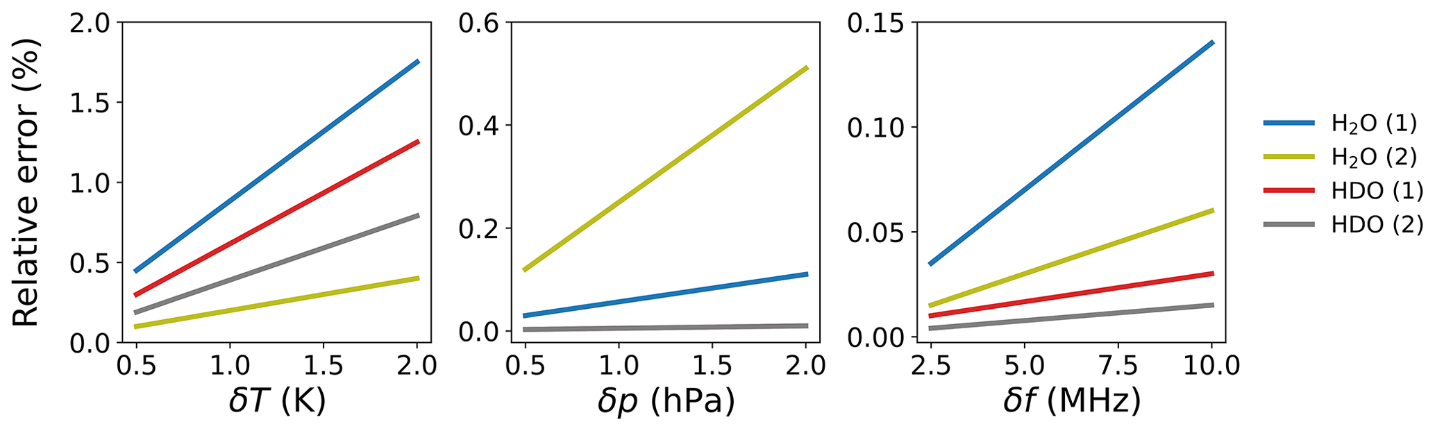
Figure 7Maximal relative error in the VMR retrieval (over 3 km range, mid-latitude baseline) due to uncertainties in the profiles of temperature (δT) and atmospheric pressure (δp) as well as transmitter on- and off-line wavelength (δf). The parenthetical numbers (1) and (2) stand for the two possible on-line wavelength options for measuring H2O.
Table 3Systematic errors for mid-latitude, arctic and tropical atmospheric models (maximal error over 3 km range). The parenthetical numbers (1) and (2) denote the two wavelength options for H2O and HDO measurements.
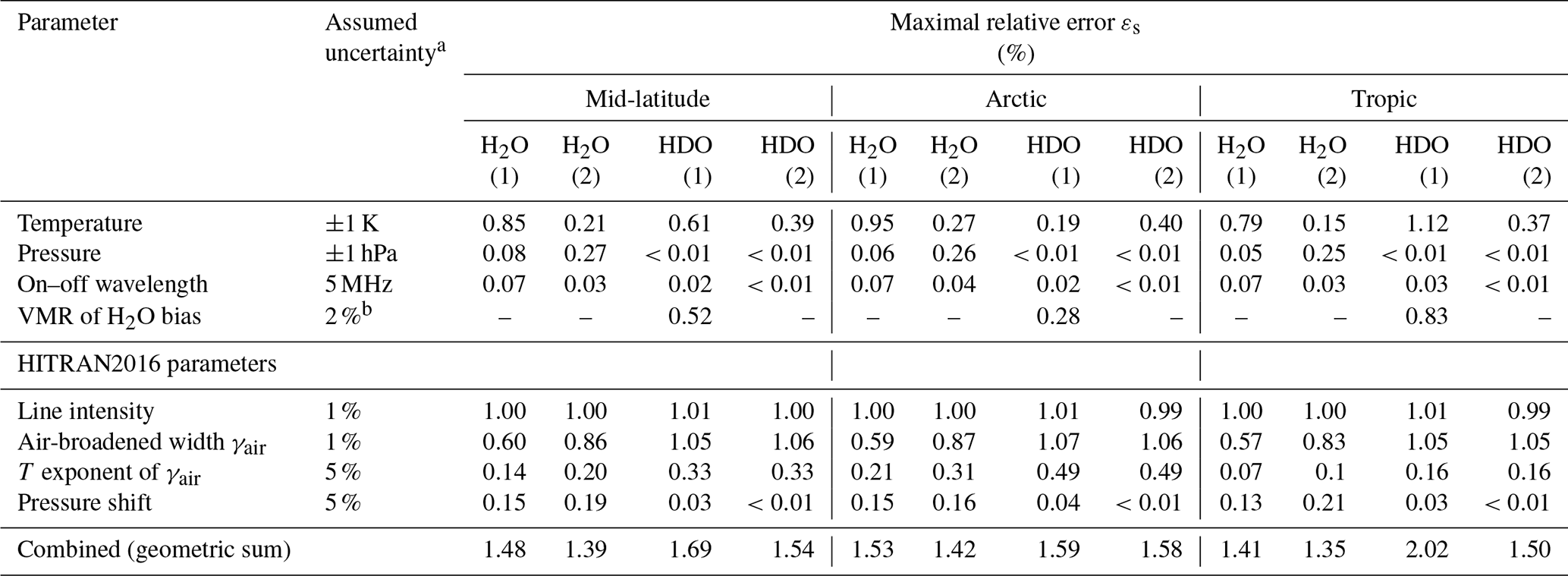
a Relative uncertainty if stated is in percent. b Conservative estimate of combined systematic error for H2O measurement.
For the case of instrument-related errors, we estimated systematic errors arising from the laser wavelength locking control and spectral quality of the laser beam. To estimate the sensitivity to laser line stability, laser frequency deviations δf ranging from 2.5 to 10 MHz were simulated. The chosen values correspond to wavelength stabilities reliably achievable over several minutes with our envisioned OPO–OPA approach coupled to a commercial wavemeter, which can suffer thermal drifts of a few megahertz over several tens of minutes. The relative wavelength error was calculated according to Eq. (16) by introducing a wavelength detuning δf to the on- and off-line wavelengths. Due to the narrower absorption line of H2O at 1982.93 nm, we find that such wavelength detuning results in a greater error compared to the spectrally larger HDO line. Option 2 for H2O measurement reduces the wavelength error. The systematic error due to the finite laser linewidth was estimated numerically by substituting the absorption cross-sections of Eq. (5) by the effective absorption cross-sections defined as
where L represents the spectral intensity distribution of the laser transmitter and ν denotes the wavenumber. The laser spectral distribution L is assumed to be an altitude-independent Gaussian function with a full width at half maximum of 50 MHz, which correlates roughly to the 10 ns pulse duration assuming transform-limited pulses. For comparison, the air-broadened Lorentzian widths of the absorption lines under standard atmospheric conditions are on the order of a few gigahertz. The calculated relative error is on the order of 0.1 % for the narrowest (thus most critical) H2O line at 1982.93 nm.
Another systematic error arises for sounding HDO at 1982.47 nm (option 2) from the insufficient knowledge of the optical depth due to the non-negligible H2O absorption feature. Assuming a relative uncertainty of 2 % in the VMR profile of H2O, which is a conservative estimate for the combined systematic error in the H2O measurement due to temperature, pressure and wavelength uncertainty, calculations reveal relative errors in the VMR retrieval varying between 0.28 % for the arctic model and 0.83 % for the tropical model. Considering this additional bias and the highly temperature sensitive H2O interference line for HDO option 1, option 2 should be the preferred wavelength option for HDO in any case. It should be noted that even for the measurement of H2O, an interference contribution due to higher HDO absorption at the off-line wavelength leads to a bias. However, this error is relatively small compared to other systematic errors and the achievable random error.
Finally, systematic errors in the VMR retrieval due to uncertainties related to spectroscopic parameters were analyzed by introducing deviations between 1 % to 5 % into the HITRAN2016 parameters of line intensity and air-broadened width and deviations of 1 % to 10 % to the temperature-dependent width coefficient and the pressure shift parameter. The resulting systematic errors are shown in Fig. 8 for each parameter. Uncertainties in parameters of line intensity and air-broadened width largely contribute to the error budget, highlighting the importance of having precise knowledge of these quantities. It should be noted that the assumed uncertainties have a rather demonstrative character as their precise quantification is still the subject of ongoing spectroscopic studies. A summary of the presented systematic errors in the form of an error budget for each of the three atmospheric models is given in Table 3.
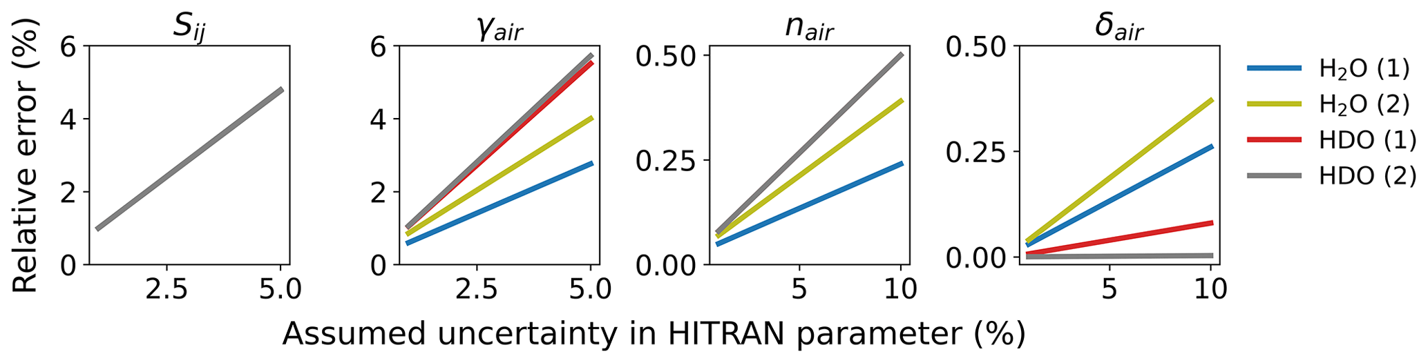
Figure 8Maximal relative error in the VMR retrieval (over 3 km range, mid-latitude baseline) due to uncertainties in HITRAN parameters. Sij: line intensity; γair: air-broadened half width; nair: coefficient of the temperature dependence of γair; δair: pressure shift.
3.4 Precision estimate applied to field campaign data
In order to complete our previous numerical studies and relate to more realistic atmospheric conditions, we present here the results of performance calculations initialized with observations obtained during the L-WAIVE (Lacustrine-Water vApor Isotope inVentory Experiment) field campaign at the Annecy lake in the French Alpine region (Chazette et al., 2021). This experiment was specifically carried out in order to obtain reference profiles that can be used to simulate the WaVIL lidar vertical profiles. Hence, the data include vertical profiles of pressure and temperature as well as vertical profiles of H2O and HDO isotopologue concentrations which were obtained by an ultra-light aircraft equipped with an in situ cavity-ring-down-spectrometer (CRDS) isotope analyzer. As aerosols were present above the planetary boundary layer on 14 June 2019, we chose data acquired from that day, ranging up to an elevation of 2.3 km. To simulate atmospheric conditions during the measurement campaign as realistically as possible, we used aerosol extinction data from the lidar WALI (Weather and Aerosol Lidar) (Chazette et al., 2014) operated during the L-WAIVE campaign on the same day (see Fig. 9a). The backscatter coefficient was estimated with a lidar ratio of 50 sr and extrapolated to a wavelength of 2 µm using the Ångström exponent derived from sun-photometer measurements. For the purpose of our simulation study, we do not take into account any measurement uncertainties in the described profiles. Figure 9b and c show the in situ-measured δD profile from the field campaign and the hypothetical precision of δD as the shaded area depending on detector characteristics and laser energy if that same profile was measured with the here-presented DIAL system (precision estimate based on wavelength option 1 for H2O and option 2 for HDO).

Figure 9(a) Experimental profiles of the water vapor mixing ratio (WVMR) and aerosol extinction coefficient (α) obtained from the L-WAIVE field campaign. Expected precision in the isotopic ratio in terms of δD for the InGaAs PIN photodetector (b) and the low-noise HgCdTe avalanche photodiode detector (c). Shaded areas indicate the absolute uncertainty based on random noise in terms of standard deviation for laser energies of 10 and 20 mJ. High uncertainty in the first 200 m is due to low signal caused by the overlap function increasing from zero to unity (see Eq. 2). Calculations are based on a measurement bandwidth of 1 MHz (150 m spatial resolution) and an integration time of 10 min.
For the commercial InGaAs PIN photodiode, the simulations show for the optimum case of 20 mJ laser energy that the uncertainty related to noise is sufficiently low for the characteristic variations in the experimentally obtained δD profile to be fully resolved with the proposed DIAL system. In terms of absolute precision, which is visualized as the width of the shaded error band around the in situ profile, δD could be determined with a precision better than 5 ‰ within the first 1.5 km and better than 10 ‰ at a range height of 2 km. A setup with 10 mJ would deliver an absolute precision close to 20 ‰ at that height. The expected precisions are on the order of or better than the columnar measurements obtained with other remote sensing techniques deployed from the ground (between 5 ‰ and 35 ‰ for a Fourier transform infrared spectrometer and the Total Carbon Column Observing Network) or from space (∼40 ‰ for the Tropospheric Emission Spectrometer and the Infrared Atmospheric Sounding Interferometer; see Table 1 of Risi et al., 2012) but with a much greater resolution on the vertical. On the other hand, the expected precision is roughly 2 to 4 times lower than for in situ airborne CRDS measurements with a similar vertical resolution (see Table 3 of Sodemann et al., 2017). Simulations performed with the HgCdTe APD indicate extremely promising precision levels over the entire range of under 3 ‰ and 5 ‰ (in absolute terms) for 20 and 10 mJ, respectively. It should be noted that the presented profiles represent a rather favorable case since the aerosol backscatter coefficient increases with altitude (due to the presence of an elevated dust layer) which is contrary to the baseline atmospheric models described in the previous numerical analysis. These simulations incorporating observed H2O and HDO profiles clearly show the potential of a ground-based DIAL instrument to measure isotopic mixing ratios with a high spatio-temporal resolution in the lower troposphere.
Probing the troposphere for water isotopologues with a high spatio-temporal resolution is of great interest to studying processes related to weather and climate, atmospheric radiation, and the hydrological cycle. In this context, the Water Vapor Isotope Lidar (WaVIL), which will measure H2O and HDO based on the differential absorption technique, is under development. The spectral window between 1982–1984 nm has been identified to perform such measurements. The selected absorption lines of H2O and HDO have a sufficiently high line strength to probe the lower 1.5 km of the atmosphere with better than 1 % relative error in the tropics and mid-latitude regions with high water vapor concentrations. The selected absorption lines are temperature sensitive, requiring accurate knowledge of the temperature profile along the line of sight for the concentration retrieval. Such a profile would have to be provided by auxiliary measurements, for example by using a Raman lidar.
We performed a sensitivity analysis and an error budget for this system taking instrument-specific and environmental parameters into account. The numerical analysis included models of mid-latitude, polar and tropical environments with realistic aerosol loads derived from the AERONET database extrapolated to the 2 µm spectral region. We showed that the retrieval of H2O and HDO mixing ratios is possible with relative random errors better than 1 % within the atmospheric boundary layer (<2 km) in mid-latitude and tropical conditions, the latter giving rise to the highest precision due to favorable differential absorption. Based on these precisions of the mixing ratio measurements, the isotopic abundance expressed in δD notation can be derived with a precision necessary to resolve vertical variations in δD of a few tens of per mil. Performance simulations also revealed differences in precision of almost 1 order of magnitude between the tropical and arctic model. Reduced precision under arctic conditions is due to low water vapor content and reduced aerosol load. These findings have been obtained for laser pulse energies of 20 mJ, a measurement bandwidth of 1 MHz (150 m range resolution), an integration time of 10 min and a commercial InGaAs PIN photodiode. As an interesting perspective option, we also investigated the theoretical performance of a state-of-the-art HgCdTe avalanche photodiode featuring an NEP reduced roughly by 1 order of magnitude. The use of such a detector would relax the requirement for laser energy and integration time and enable high-precision, range-resolved measurement of the isotopic ratio.
An error budget has been performed to outline systematic errors due to uncertainties in atmospheric-, spectroscopic- and instrument-related parameters. The H2O on-line wavelength at 1982.93 nm shows a pronounced temperature sensitivity imposing strict requirements on accurate temperature profiles for the VMR retrieval. This can be mitigated by tuning the on-line wavelength to 1982.97 nm which, however, comes at the cost of slightly increased pressure sensitivity and slightly reduced differential absorption. For the HDO isotopologue, two wavelength options have been studied. Option 2 with the on-line wavelength at 1983.93 nm was found to be more suitable since it has no H2O interference (as is the case for HDO option 1 at 1982.47 nm). The slightly smaller differential absorption for option 2 is a price worth paying, and the resulting increase in random error can be offset by longer signal averaging. Including systematic errors due to inexact spectroscopic parameters in our analysis, we highlighted the importance of accurate knowledge of them for DIAL measurements and the necessity for ongoing spectroscopic studies of water vapor isotopologues in the 2 µm region.
Finally, using a measured H2O−HDO profile obtained during the recent L-WAIVE field campaign, our calculations have shown that sufficient precision in the mixing ratios of H2O and HDO can be achieved with the presented system parameters so that characteristic, vertical variations in the isotopic content δD observed during the field campaign could be resolved with the proposed DIAL system, showing the potential to complement existing methods. Although an effort has been made to conduct the sensitivity analysis and error budget as thoroughly as possible, it should be nevertheless noted that the predicted performance of the presented DIAL system can be understood as a best-case scenario. Assumptions made for the transmitter model, such as no laser beam pointing or perfect spectral purity, are very challenging aspects in actual laser development. Future work will consist of improving our knowledge of the spectroscopy of HDO in the 1982–1984 nm spectral region and testing the DIAL system in the framework of a forthcoming field campaign.
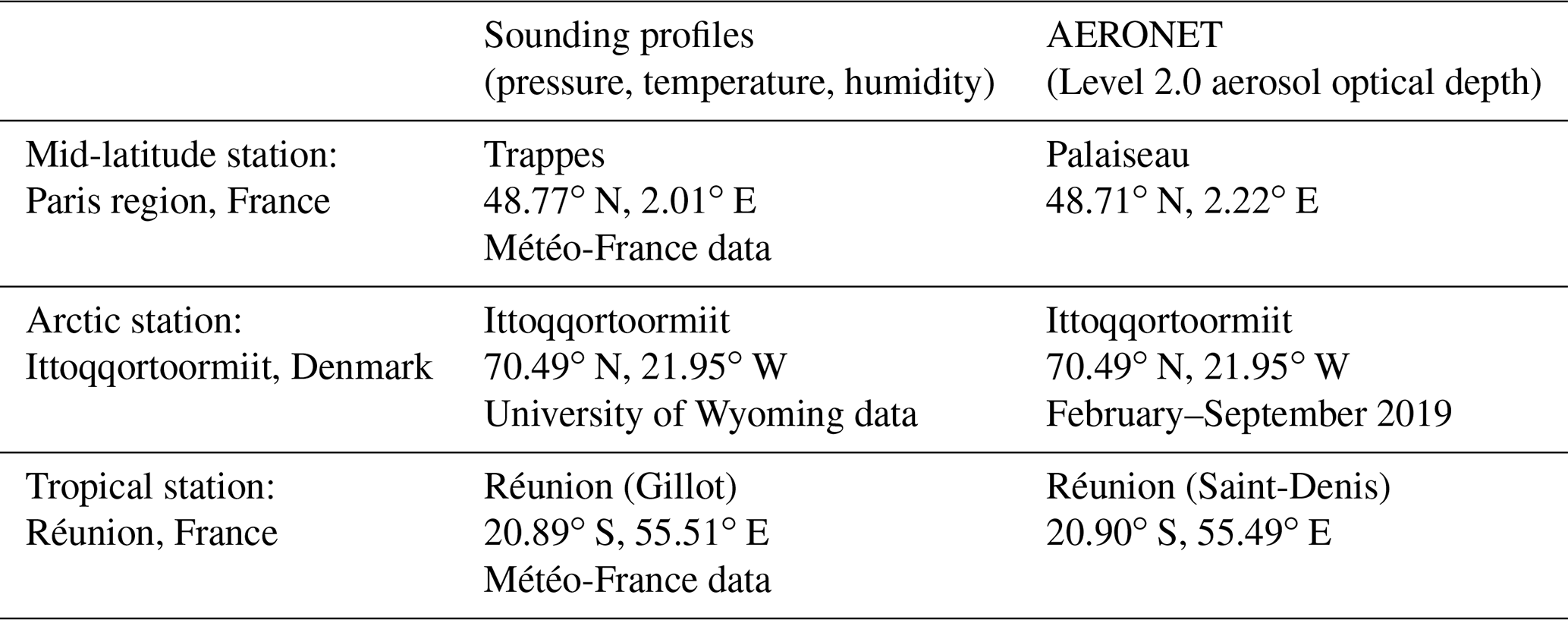
Table A1 lists databases and locations used to derive the three atmospheric models discussed in this paper. Available data from the year of 2019 were used for all locations.
Table A1Overview of atmospheric sounding and AERONET sites used to derive an atmosphere model for the sensitivity analysis. For all sites data from 2019 were used. Note that for the arctic station, AERONET photometer products are from February until September.
Simulation code can be requested from the lead author (jonas.hamperl@onera.fr).
The meteorological sounding data used for this study are publicly available from the University of Wyoming (http://weather.uwyo.edu/upperair/sounding.html, last access: 4 October 2021) and from the French national meteorological service Météo-France (https://donneespubliques.meteofrance.fr, last access: 4 October 2021). Aerosol optical depth data can be accessed via the AERONET website (https://aeronet.gsfc.nasa.gov/, last access: 4 October 2021; Holben et al., 1998, https://doi.org/10.1016/S0034-4257(98)00031-5). Raw data can be given upon request.
JH, J-BD, MR, RS, AG, J-MM, JT, PC and CF conceptualized the measurement concept; JH was responsible for the lidar performance simulator; HS, AS, JT and PC curated the L-WAIVE campaign data; LR, CC, MR and JH wrote the original draft of the manuscript, and all authors contributed to review and editing; CF and CE were responsible for project administration; all authors have read and agreed to the published version of the paper.
The contact author has declared that neither they nor their co-authors have any competing interests.
Publisher's note: Copernicus Publications remains neutral with regard to jurisdictional claims in published maps and institutional affiliations.
The authors would like to thank the AERONET network and responsible principal investigators (PIs) for sun-photometer products. The authors acknowledge the provision of meteorological sounding data by the University of Wyoming and the French national meteorological service Météo-France.
The authors would like to thank the ANR and have received funding from the European Union's Horizon 2020 research and innovation program. Harald Sodemann and Andrew Seidl acknowledge funding obtained through ERC Consolidator Grants.
This research has been supported by the Agence Nationale de la Recherche (grant no. ANR-16-CE01-0009) and the European Research Council's Horizon 2020 funding scheme via the LEMON project (grant no. 821868) and the ISLAS project (grant no. 773245).
This paper was edited by John Sullivan and reviewed by two anonymous referees.
AERONET: Aerosol optical depth data, available at: https://aeronet.gsfc.nasa.gov/, last access: 4 October 2021.
Agence Nationale de la Recherche: Differential absorption lidar for monitoring water vapour isotope HDO in the lower troposphere – WaVIL, available at: https://anr.fr/Project-ANR-16-CE01-0009 (last access: 12 March 2021).
Ångström, A.: On the Atmospheric Transmission of Sun Radiation and on Dust in the Air, Geogr. Ann., 11, 156–166, https://doi.org/10.1080/20014422.1929.11880498, 1929.
Ansmann, A., Bösenberg, J., Chaikovsky, A., Comerón, A., Eckhardt, S., Eixmann, R., Freudenthaler, V., Ginoux, P., Komguem, L., Linné, H., Márquez, M. Á. L., Matthias, V., Mattis, I., Mitev, V., Müller, D., Music, S., Nickovic, S., Pelon, J., Sauvage, L., Sobolewsky, P., Srivastava, M. K., Stohl, A., Torres, O., Vaughan, G., Wandinger, U., and Wiegner, M.: Long-Range Transport of Saharan Dust to Northern Europe: The 11–16 October 2001 Outbreak Observed with EARLINET, J. Geophys. Res.-Atmos., 108, 4783, https://doi.org/10.1029/2003JD003757, 2003.
Barrientos Barria, J., Mammez, D., Cadiou, E., Dherbecourt, J. B., Raybaut, M., Schmid, T., Bresson, A., Melkonian, J. M., Godard, A., Pelon, J., and Lefebvre, M.: Multispecies High-Energy Emitter for CO2, CH4, and H2O Monitoring in the 2 µm Range, Opt. Lett., 39, 6719–6722, https://doi.org/10.1364/OL.39.006719, 2014.
Bösenberg, J.: Differential-Absorption Lidar for Water Vapor and Temperature Profiling, in: Lidar: Range-Resolved Optical Remote Sensing of the Atmosphere, Springer Series in Optical Sciences, edited by: Weitkamp, C., Springer, New York, NY, 213–239, https://doi.org/10.1007/0-387-25101-4_8, 2005.
Browell, E., Ismail, S., and Grossmann, B.: Temperature sensitivity of differential absorption lidar measurements of water vapor in the 720 nm region, Appl. Optics, 30, 1517–1524, 1991.
Bruneau, D., Quaglia, P., Flamant, C., Meissonnier, M., and Pelon, J.: Airborne Lidar LEANDRE II for Water-Vapor Profiling in the Troposphere. I. System Description, Appl. Optics, 40, 3450–3461, https://doi.org/10.1364/AO.40.003450, 2001.
Cadiou, E., Dherbecourt, J.-B., Gorju, G., Raybaut, M., Melkonian, J.-M., Godard, A., Pelon, J., and Lefebvre, M.: 2-µm Direct Detection Differential Absorption LIDAR For Multi-Species Atmospheric Sensing, in: Conference on Lasers and Electro-Optics (2016), San Jose, United States, 5–10 June 201; Optical Society of America, p STh1H.2, https://doi.org/10.1364/CLEO_SI.2016.STh1H.2, 2016.
Chazette, P. and Royer, P.: Springtime Major Pollution Events by Aerosol over Paris Area: From a Case Study to a Multiannual Analysis, J. Geophys. Res.-Atmos., 122, 8101–8119, https://doi.org/10.1002/2017JD026713, 2017.
Chazette, P., Marnas, F., and Totems, J.: The mobile Water vapor Aerosol Raman LIdar and its implication in the framework of the HyMeX and ChArMEx programs: application to a dust transport process, Atmos. Meas. Tech., 7, 1629–1647, https://doi.org/10.5194/amt-7-1629-2014, 2014.
Chazette, P., Totems, J., and Shang, X.: Atmospheric Aerosol Variability above the Paris Area during the 2015 Heat Wave – Comparison with the 2003 and 2006 Heat Waves, Atmos. Environ., 170, 216–233, https://doi.org/10.1016/j.atmosenv.2017.09.055, 2017.
Chazette, P., Raut, J.-C., and Totems, J.: Springtime aerosol load as observed from ground-based and airborne lidars over northern Norway, Atmos. Chem. Phys., 18, 13075–13095, https://doi.org/10.5194/acp-18-13075-2018, 2018.
Chazette, P., Flamant, C., Sodemann, H., Totems, J., Monod, A., Dieudonné, E., Baron, A., Seidl, A., Steen-Larsen, H. C., Doira, P., Durand, A., and Ravier, S.: Experimental investigation of the stable water isotope distribution in an Alpine lake environment (L-WAIVE), Atmos. Chem. Phys., 21, 10911–10937, https://doi.org/10.5194/acp-21-10911-2021, 2021.
Collis, R. T. H. and Russell, P. B.: Lidar Measurement of Particles and Gases by Elastic Backscattering and Differential Absorption, in: Laser Monitoring of the Atmosphere, Topics in Applied Physics, edited by: Hinkley, E. D., Springer, Berlin, Heidelberg, 71–151, https://doi.org/10.1007/3-540-07743-X_18, 1976.
Craig, H.: Standard for Reporting Concentrations of Deuterium and Oxygen-18 in Natural Waters, Science, 133, 1833–1834, https://doi.org/10.1126/science.133.3467.1833, 1961.
Di Pierro, M., Jaeglé, L., Eloranta, E. W., and Sharma, S.: Spatial and seasonal distribution of Arctic aerosols observed by the CALIOP satellite instrument (2006–2012), Atmos. Chem. Phys., 13, 7075–7095, https://doi.org/10.5194/acp-13-7075-2013, 2013.
Ehret, G., Kiemle, C., Wirth, M., Amediek, A., Fix, A., and Houweling, S.: Space-Borne Remote Sensing of CO2, CH4, and N2O by Integrated Path Differential Absorption Lidar: A Sensitivity Analysis, Appl. Phys. B, 90, 593–608, https://doi.org/10.1007/s00340-007-2892-3, 2008.
European Space Agency: ARMA Reference Model of the Atmosphere, in: Technical Report APP-FP/99-11239/AC/ac, 1999.
Galewsky, J., Steen-Larsen, H. C., Field, R. D., Worden, J., Risi, C., and Schneider, M.: Stable Isotopes in Atmospheric Water Vapor and Applications to the Hydrologic Cycle, Rev. Geophys., 54, 809–865, https://doi.org/10.1002/2015RG000512, 2016.
Geng, J. and Jiang, S.: Fiber Lasers: The 2 µm Market Heats Up, Opt. Photonics News, 25, 34–41, https://doi.org/10.1364/OPN.25.7.000034, 2014.
Gibert, F., Dumas, A., Rothman, J., Edouart, D., Cénac, C., and Pellegrino, J.: Performances of a HgCdTe APD Based Direct Detection Lidar at 2 µm, Application to Dial Measurements, EPJ Web Conf., 176, 01001, https://doi.org/10.1051/epjconf/201817601001, 2018.
Godard, A.: Infrared (2–12 µm) Solid-State Laser Sources: A Review, C. R. Phys., 8, 1100–1128, https://doi.org/10.1016/j.crhy.2007.09.010, 2007.
Gordon, I. E., Rothman, L. S., Hill, C., Kochanov, R. V., Tan, Y., Bernath, P. F., Birk, M., Boudon, V., Campargue, A., Chance, K. V., Drouin, B. J., Flaud, J.-M., Gamache, R. R., Hodges, J. T., Jacquemart, D., Perevalov, V. I.; Perrin, A., Shine, K. P., Smith, M.-A. H., Tennyson, J., Toon, G. C., Tran, H., Tyuterev, V. G., Barbe, A., Császár, A. G., Devi, V. M., Furtenbacher, T., Harrison, J. J., Hartmann, J.-M., Jolly, A., Johnson, T. J., Karman, T., Kleiner, I., Kyuberis, A. A., Loos, J., Lyulin, O. M., Massie, S. T., Mikhailenko, S. N., Moazzen-Ahmadi, N., Müller, H. S. P., Naumenko, O. V., Nikitin, A. V., Polyansky, O. L., Rey, M., Rotger, M., Sharpe, S. W., Sung, K., Starikova, E., Tashkun, S. A., Auwera, J. V., Wagner, G., Wilzewski, J., Wcisło, P., Yu, S., and Zak, E. J.: The HITRAN2016 Molecular Spectroscopic Database, J. Quant. Spectrosc. Ra., 203, 3–69, https://doi.org/10.1016/j.jqsrt.2017.06.038, 2017.
Hamperl, J., Capitaine, C., Santagata, R., Dherbecourt, J.-B., Melkonian, J.-M., Godard, A., Raybaut, M., Régalia, L., Grouiez, B., Blouzon, F., Geyskens, N., Evesque, C., Chazette, P., Totems, J., and Flamant, C.: WaVIL: A Differential Absorption LIDAR for Water Vapor and Isotope HDO Observation in the Lower Troposphere – Instrument Design, in: Optical Sensors and Sensing Congress, Washington, DC, United States, 22–26 June 2020, paper LM4A.4; Optical Society of America, 2020.
Holben, B. N., Eck, T. F., Slutsker, I., Tanré, D., Buis, J. P., Setzer, A., Vermote, E., Reagan, J. A., Kaufman, Y. J., Nakajima, T., Lavenu, F., Jankowiak, I., and Smirnov, A.: Aeronet—A Federated Instrument Network and Data Archive for Aerosol Characterization, Remote Sens. Environ., 66, 1–16, https://doi.org/10.1016/S0034-4257(98)00031-5, 1998 (data vailable at: https://aeronet.gsfc.nasa.gov/, last access: 4 October 2021).
Matthias, V., Balis, D., Bösenberg, J., Eixmann, R., Iarlori, M., Komguem, L., Mattis, I., Papayannis, A., Pappalardo, G., Perrone, M. R., and Wang, X.: Vertical Aerosol Distribution over Europe: Statistical Analysis of Raman Lidar Data from 10 European Aerosol Research Lidar Network (EARLINET) Stations, J. Geophys. Res., 109, D18201, https://doi.org/10.1029/2004JD004638, 2004.
Refaat, T. F., Singh, U. N., Yu, J., Petros, M., Ismail, S., Kavaya, M. J., and Davis, K. J.: Evaluation of an Airborne Triple-Pulsed 2 µm IPDA Lidar for Simultaneous and Independent Atmospheric Water Vapor and Carbon Dioxide Measurements, Appl. Optics, 54, 1387–1398, https://doi.org/10.1364/AO.54.001387, 2015.
Risi, C., Noone, D., Worden, J., Frankenberg, C., Stiller, G., Kiefer, M., Funke, B., Walker, K., Bernath, P., Schneider, M., Bony, S., Lee, J., Brown, D., and Sturm, C.: Process-evaluation of tropospheric humidity simulated by general circulation models using water vapor isotopic observations: 2. Using isotopic diagnostics to understand the mid and upper tropospheric moist bias in the tropics and subtropics, J. Geophys. Res., 117, D05304, https://doi.org/10.1029/2011JD016623, 2012.
Singh, U. N., Refaat, T. F., Ismail, S., Davis, K. J., Kawa, S. R., Menzies, R. T., and Petros, M.: Feasibility Study of a Space-Based High Pulse Energy 2 µm CO2 IPDA Lidar, Appl. Optics, 56, 6531–6547, https://doi.org/10.1364/AO.56.006531, 2017.
Spuler, S. M., Repasky, K. S., Morley, B., Moen, D., Hayman, M., and Nehrir, A. R.: Field-deployable diode-laser-based differential absorption lidar (DIAL) for profiling water vapor, Atmos. Meas. Tech., 8, 1073–1087, https://doi.org/10.5194/amt-8-1073-2015, 2015.
Sodemann, H., Aemisegger, F., Pfahl, S., Bitter, M., Corsmeier, U., Feuerle, T., Graf, P., Hankers, R., Hsiao, G., Schulz, H., Wieser, A., and Wernli, H.: The stable isotopic composition of water vapour above Corsica during the HyMeX SOP1 campaign: insight into vertical mixing processes from lower-tropospheric survey flights, Atmos. Chem. Phys., 17, 6125–6151, https://doi.org/10.5194/acp-17-6125-2017, 2017.
Stevens, B. and Bony, S.: Water in the Atmosphere, Phys. Today, 66, 6, 29–34, https://doi.org/10.1063/PT.3.2009, 2013.
Tomasi, C., Kokhanovsky, A. A., Lupi, A., Ritter, C., Smirnov, A., O'Neill, N. T., Stone, R. S., Holben, B. N., Nyeki, S., Wehrli, C., Stohl, A., Mazzola, M., Lanconelli, C., Vitale, V., Stebel, K., Aaltonen, V., de Leeuw, G., Rodriguez, E., Herber, A. B., Radionov, V. F., Zielinski, T., Petelski, T., Sakerin, S. M., Kabanov, D. M., Xue, Y., Mei, L., Istomina, L., Wagener, R., McArthur, B., Sobolewski, P. S., Kivi, R., Courcoux, Y., Larouche, P., Broccardo, S., and Piketh, S. J.: Aerosol Remote Sensing in Polar Regions, Earth-Sci. Rev., 140, 108–157, https://doi.org/10.1016/j.earscirev.2014.11.001, 2015.
Wagner, G. A. and Plusquellic, D. F.: Multi-Frequency Differential Absorption LIDAR System for Remote Sensing of CO2 and H2O near 1.6 µm, Opt. Express, 26, 19420–19434, https://doi.org/10.1364/OE.26.019420, 2018.
Wandinger, U.: Raman Lidar, in: Lidar: Range-Resolved Optical Remote Sensing of the Atmosphere, Springer Series in Optical Sciences, edited by: Weitkamp, C., Springer, New York, NY, 241–271, https://doi.org/10.1007/0-387-25101-4_9, 2005.
Whiteman, D. N., Melfi, S. H., and Ferrare, R. A.: Raman Lidar System for the Measurement of Water Vapor and Aerosols in the Earth's Atmosphere, Appl. Optics, 31, 3068–3082, https://doi.org/10.1364/AO.31.003068, 1992.
Winker, D. M., Tackett, J. L., Getzewich, B. J., Liu, Z., Vaughan, M. A., and Rogers, R. R.: The global 3-D distribution of tropospheric aerosols as characterized by CALIOP, Atmos. Chem. Phys., 13, 3345–3361, https://doi.org/10.5194/acp-13-3345-2013, 2013.
Wirth, M., Fix, A., Mahnke, P., Schwarzer, H., Schrandt, F., and Ehret, G.: The Airborne Multi-Wavelength Water Vapor Differential Absorption Lidar WALES: System Design and Performance, Appl. Phys. B, 96, 201, https://doi.org/10.1007/s00340-009-3365-7, 2009.
- Abstract
- Introduction
- DIAL method and performance model for water vapor isotopologue measurement
- Simulation results and discussion
- Conclusions
- Appendix A
- Code availability
- Data availability
- Author contributions
- Competing interests
- Disclaimer
- Acknowledgements
- Financial support
- Review statement
- References