Can a regional-scale reduction of atmospheric CO<sub>2</sub> during the COVID-19 pandemic be detected from space? A case study for East China using satellite XCO<sub>2</sub> retrievals

Buchwitz, Michael; Reuter, Maximilian; Noël, Stefan; Bramstedt, Klaus; Schneising, Oliver; Hilker, Michael; Fuentes Andrade, Blanca; Bovensmann, Heinrich; Burrows, John P.; Di Noia, Antonio; Boesch, Hartmut; Wu, Lianghai; Landgraf, Jochen; Aben, Ilse; Retscher, Christian; O'Dell, Christopher W.; Crisp, David

doi:https://doi.org/10.5194/amt-14-2141-2021

Articles | Volume 14, issue 3

https://doi.org/10.5194/amt-14-2141-2021

Articles | Volume 14, issue 3

Research article

18 Mar 2021

Research article |

| 18 Mar 2021

Can a regional-scale reduction of atmospheric CO₂ during the COVID-19 pandemic be detected from space? A case study for East China using satellite XCO₂ retrievals

Michael Buchwitz, Maximilian Reuter, Stefan Noël, Klaus Bramstedt, Oliver Schneising, Michael Hilker, Blanca Fuentes Andrade, Heinrich Bovensmann, John P. Burrows, Antonio Di Noia, Hartmut Boesch, Lianghai Wu, Jochen Landgraf, Ilse Aben, Christian Retscher, Christopher W. O'Dell, and David Crisp

Abstract

The COVID-19 pandemic resulted in reduced anthropogenic carbon dioxide (CO₂) emissions during 2020 in large parts of the world. To investigate whether a regional-scale reduction of anthropogenic CO₂ emissions during the COVID-19 pandemic can be detected using space-based observations of atmospheric CO₂, we have analysed a small ensemble of OCO-2 and GOSAT satellite retrievals of column-averaged dry-air mole fractions of CO₂, i.e. XCO₂. We focus on East China and use a simple data-driven analysis method. We present estimates of the relative change of East China monthly emissions in 2020 relative to previous periods, limiting the analysis to October-to-May periods to minimize the impact of biogenic CO₂ fluxes. The ensemble mean indicates an emission reduction by approximately 10 % ± 10 % in March and April 2020. However, our results show considerable month-to-month variability and significant differences across the ensemble of satellite data products analysed. For example, OCO-2 suggests a much smaller reduction (∼ 1 %–2 % ± 2 %). This indicates that it is challenging to reliably detect and to accurately quantify the emission reduction with current satellite data sets. There are several reasons for this, including the sparseness of the satellite data but also the weak signal; the expected regional XCO₂ reduction is only on the order of 0.1–0.2 ppm. Inferring COVID-19-related information on regional-scale CO₂ emissions using current satellite XCO₂ retrievals likely requires, if at all possible, a more sophisticated analysis method including detailed transport modelling and considering a priori information on anthropogenic and natural CO₂ surface fluxes.

Download & links

How to cite.

Buchwitz, M., Reuter, M., Noël, S., Bramstedt, K., Schneising, O., Hilker, M., Fuentes Andrade, B., Bovensmann, H., Burrows, J. P., Di Noia, A., Boesch, H., Wu, L., Landgraf, J., Aben, I., Retscher, C., O'Dell, C. W., and Crisp, D.: Can a regional-scale reduction of atmospheric CO₂ during the COVID-19 pandemic be detected from space? A case study for East China using satellite XCO₂ retrievals, Atmos. Meas. Tech., 14, 2141–2166, https://doi.org/10.5194/amt-14-2141-2021, 2021.

Received: 24 Sep 2020 – Discussion started: 08 Oct 2020 – Revised: 10 Feb 2021 – Accepted: 11 Feb 2021 – Published: 18 Mar 2021

1 Introduction

Carbon dioxide (CO₂) is the most important anthropogenic greenhouse gas significantly contributing to global warming (IPCC, 2013). CO₂ has many natural and anthropogenic sources and sinks, and our current understanding of them has significant gaps (e.g. Ciais et al., 2014; Chevallier et al., 2014; Reuter et al., 2017c; Crisp et al., 2018; Friedlingstein et al., 2019). Efforts are ongoing to improve the fundamental understanding of the global carbon cycle, to improve our ability to project future changes and to verify the effectiveness of policies such as the Paris Agreement (https://unfccc.int/process-and-meetings/the-paris-agreement/the-paris-agreement, last access: 8 September 2020) aiming to reduce greenhouse gas emissions (e.g. Ciais et al., 2014, 2015; Pinty et al., 2017, 2019; Crisp et al., 2018; Matsunaga and Maksyutov, 2018; Janssens-Maenhout et al., 2020).

Retrievals of XCO₂ from the satellite sensors SCIAMACHY/ENVISAT (Burrows et al., 1995; Bovensmann et al., 1999; Reuter et al., 2010, 2011) and TANSO-FTS/GOSAT (Kuze et al., 2016) and from the Orbiting Carbon Observatory-2 (OCO-2) satellite (Crisp et al., 2004; Eldering et al., 2017; O'Dell et al., 2012, 2018) have been used in recent years to obtain information on natural CO₂ sources and sinks (e.g. Basu et al., 2013; Chevallier et al., 2014; Chevallier, 2015; Reuter et al., 2014a, 2017c; Schneising et al., 2014; Houweling et al., 2015; Kaminski et al., 2017; Liu et al., 2017; Eldering et al., 2017; Yin et al., 2018; Palmer et al., 2019; Miller and Michalak, 2020), on anthropogenic CO₂ emissions (e.g. Schneising et al., 2008, 2013; Reuter et al., 2014b, 2019; Nassar et al., 2017; Schwandner et al., 2017; Matsunaga and Maksyutov, 2018; Miller et al., 2019; Labzovskii et al., 2019; Wu et al., 2020; Zheng et al., 2020a; Ye et al., 2020), and for other applications such as climate model assessments (e.g. Lauer et al., 2017; Gier et al., 2020) or data assimilation (e.g. Massart et al., 2016).

Here we use an ensemble of satellite retrievals of XCO₂ to determine whether COVID-19-related regional-scale (here ∼ 2000² km²) CO₂ emission reductions can be detected and quantified using the current space-based observing system. This is important in order to establish the capabilities of current satellites, which have been optimized to obtain information on natural carbon sources and sinks but not to obtain information on anthropogenic emissions. Nevertheless, data from existing satellites have already been used to assess anthropogenic emissions (see publications cited above). These assessments and the assessment presented in this publication are relevant for future satellites focussing on anthropogenic emissions, such as the planned European Copernicus Anthropogenic CO₂ Monitoring (CO2M) mission (e.g. ESA, 2019; Kuhlmann et al., 2019; Janssens-Maenhout et al., 2020), which is based on the CarbonSat concept (Bovensmann et al., 2010; Velazco et al., 2011; Buchwitz et al., 2013; Pillai et al., 2016; Broquet et al., 2018; Lespinas et al., 2020).

We focus on China because regional-scale COVID-19-related CO₂ emission reductions are expected to be largest there early in the pandemic (Le Quéré et al., 2020; Liu et al., 2020). Satellite data have been used to estimate China's CO₂ emissions during the COVID-19 pandemic as shown in Zheng et al. (2020b), but that study inferred CO₂ reductions from retrievals of nitrogen dioxide (NO₂) not using XCO₂. Estimates of emission reductions have also been derived from bottom-up statistical assessments of fossil fuel use and other economic indicators. According to Le Quéré et al. (2020), China's CO₂ emissions decreased by 242 Mt CO₂ (uncertainty range 108–394 Mt CO₂) during January–April 2020. As China's annual CO₂ emissions are approximately 10 Gt CO₂ yr⁻¹ (Friedlingstein et al., 2019), i.e. approximately 3.3 Gt CO₂ in a 4-month period assuming constant emissions, the average relative (COVID-19 related) change during January–April 2020 is therefore approximately 7 % ± 4 % (0.242/3.3 ± 0.14/3.3). This agrees reasonably well with the estimate reported in Liu et al. (2020), which is 9.3 % for China during the first quarter of 2020 compared to the same period in 2019. Liu et al. (2020) also indicate some challenges in terms of interpreting CO₂ emission reductions as being caused by COVID-19, e.g. the fact that the first months of 2020 were exceptionally warm across much of the Northern Hemisphere. CO₂ emissions associated with home heating may have therefore been somewhat lower than for the same period in 2019, even without the disruption in economic activities and energy production caused by COVID-19 and related lockdowns.

Sussmann and Rettinger (2020) studied ground-based remote-sensing XCO₂ retrievals of the Total Carbon Column Observing Network (TCCON) to find out whether related atmospheric concentration changes may be detected by the TCCON and brought into agreement with bottom-up emission-reduction estimates. Our study is one of the first attempts to determine whether COVID-19-related regional-scale CO₂ emission reductions can be detected using existing space-based observations of XCO₂. Tohjima et al. (2020) inferred estimates of China's CO₂ emissions from modelled and observed ratios of CO₂ and methane (CH₄) surface concentrations at Hateruma Island, Japan. They report for China fossil fuel emission reductions of 32 ± 12 % and 19 ± 15 % for February and March 2020, respectively, which is about 10 % higher compared to the results shown in Le Quéré et al., 2020 (see Table 1 of Tohjima et al., 2020). From model sensitivity simulations they conclude that even a 30 % reduction of China's fossil fuel CO₂ emissions would only result in a 0.8 ppm XCO₂ reduction over China and that it therefore would be very challenging to detect any COVID-19-related signal with the existing remote-sensing satellites GOSAT and OCO-2. Their conjecture has essentially been confirmed by Chevallier et al. (2020). They used XCO₂ from OCO-2 in combination with other data sets and the modelling of CO₂ emission plumes of localized CO₂ sources to obtain estimates of CO₂ emissions focussing on several COVID-19-relevant regions such as China, Europe, India and the USA. They concluded that these places have not been well observed by the OCO-2 satellite because of frequent or persistent cloud conditions and they give recommendations for future carbon-monitoring systems. Zeng et al. (2020) used modelling, GOSAT XCO₂ and other data sets. They conclude that GOSAT is able to detect a short-term global mean XCO₂ anomaly decrease of 0.2–0.3 ppm after temporal averaging (e.g. monthly), but for East China they could not identify a statistically robust COVID-19-related anomaly. Satellite-derived results related to this application are also provided in the internet (e.g. ESA-NASA-JAXA, 2020).

Regional-scale reductions of tropospheric NO₂ columns have been reported for China (e.g. Zhang et al., 2020; Bauwens et al., 2020), but for CO₂ such an assessment is more challenging because of small XCO₂ changes on top of a large background. For example, over extended anthropogenic source areas such as East China, the XCO₂ enhancement due to anthropogenic emissions is typically only approximately 1–2 ppm (0.25 %–0.5 % of 400 ppm) or even less (see e.g. Schneising et al., 2008, 2013; Hakkarainen et al., 2016, 2019; Chevallier et al., 2020; Tohjima et al., 2020; and this study). A 10 % emission reduction would therefore only change the regional XCO₂ enhancement by 0.1 to 0.2 ppm. This is below the single measurement precision of current satellite XCO₂ data products (at footprint size, i.e. 10.5 km diameter for GOSAT (Kuze et al., 2016) and 1.3 × 2.3 km² for OCO-2 (O'Dell et al., 2018)), which is about 1.8 ppm (1σ) (e.g. Dils et al., 2014; Kulawik et al., 2016; Buchwitz et al., 2015, 2017a; Reuter et al., 2020) for GOSAT and around 1 ppm for OCO-2 (Wunch et al., 2017; Reuter et al., 2019). In our study we focus on XCO₂ monthly averages. Averaging reduces the noise of the satellite retrievals (e.g. Kulawik et al., 2016) but also eliminates day-to-day XCO₂ variations (e.g. Agustí-Panareda et al., 2019), which cannot be interpreted using our simple analysis methods. The accuracy of the East China satellite XCO₂ retrievals averaged over monthly timescales is difficult to assess because of limited reference data. The validation of the satellite data products is primarily based on comparisons with ground-based XCO₂ retrievals from the TCCON, a relatively sparse network with an uncertainty of about 0.4 ppm (Wunch et al., 2010).

The purpose of this study is to investigate – using satellite XCO₂ retrievals – if satellite-derived East China fossil fuel (FF) CO₂ emissions in 2020 (COVID-19 period) differ significantly compared to pre-COVID-19 periods. Ideally, we would like to know by how much emissions have been reduced due to COVID-19. This question, however, cannot be answered using only satellite data because they do not contain any information on how much would have been emitted without COVID-19. Instead, we aim at answering the following question: are satellite-derived East China FF CO₂ emissions early in the pandemic (here: January–May 2020) significantly lower compared to pre-COVID-19 periods?

To answer this question, we analyse relative differences of estimates of East China monthly FF emissions during different time periods. We focus on October-to-May periods, and we refer to different periods via the year where a period ends; i.e. we call the period October 2019 to May 2020 “year 2020 period” or simply “2020”, the period October 2018 to May 2019 is called 2019, etc. Specifically, we compute and analyse differences of monthly emissions in the year 2020 period relative to previous year 2016 to 2019 periods; i.e. we use four periods for comparison with the year 2020 period. To focus on the COVID-19 aspect, we subtract for each period the October-to-December (OND) mean value, and we refer to these time series as “OND anomalies”. These OND anomalies are time series at monthly resolution of the relative emission difference between different periods relative to OND. Negative OND anomalies during the COVID-19 period would then suggest (depending on uncertainty) that an emission reduction during the COVID-19 period has been detected.

The structure of our paper reflects this procedure: in the Data section (Sect. 2) we present the satellite and model input data used for this study. In the Methods section (Sect. 3) we present the analysis method, which consists of two main steps. The purpose of the first step is to isolate the East China FF emission signal from the XCO₂ satellite retrievals. This is done by subtracting appropriate XCO₂ background values from the XCO₂ retrievals to obtain XCO₂ anomalies, ΔXCO₂. We use two methods to compute ΔXCO₂. We describe one method, the DAM method, in detail in Sect. 3.1 and only shortly explain the second method (TmS method), referring for details to Appendix A. In the second step (Sect. 3.2) we compute estimates of East China monthly FF CO₂ emissions from the XCO₂ anomalies. These emission estimates are then used to compute the OND anomalies explained above. In Results and discussion section (Sect. 4) we present and discuss the results, i.e. the application of the described methods to the satellite data. A summary and conclusions are given in Sect. 5.

2 Data

In this section, we present a short overview about the input data used for this study.

2.1 Satellite XCO₂ retrievals

This study uses four satellite XCO₂ Level 2 (L2) data products. An overview about these data sets is provided in Table 1. The first product listed in Table 1 is the latest version of the bias-corrected OCO-2 XCO₂ product delivered to the Goddard Earth Science Data and Information Services Center (GES DISC) by the OCO-2 team (ACOS v10r Lite). The other three satellite XCO₂ data sets are different versions of the GOSAT XCO₂ product derived using retrieval algorithms developed by groups at the University of Leicester, UK (UoL-FP v7.3); the SRON Netherlands Institute for Space Research (RemoTeC v2.3.8); and the University of Bremen, Germany (FOCAL v1.0).

Table 1Overview of the satellite XCO₂ Level 2 (L2) input data products.

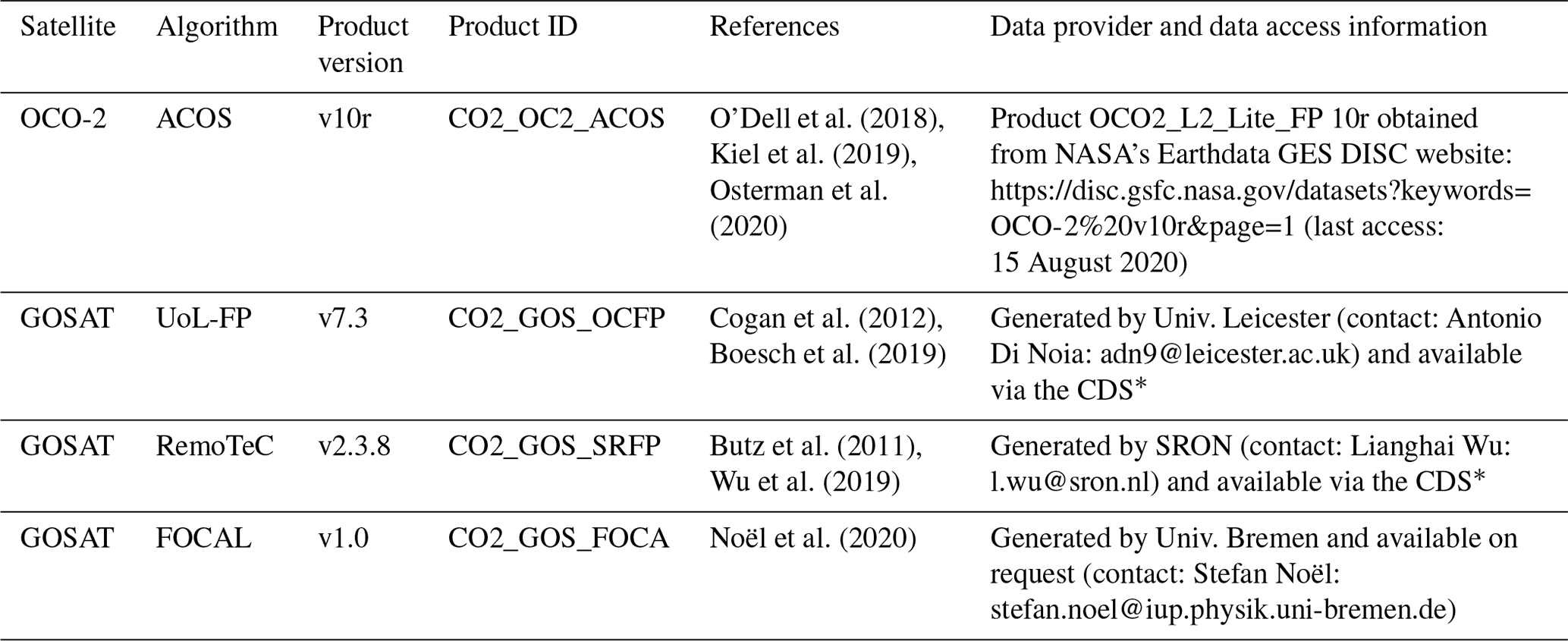
^∗ Products are available via the Copernicus Climate Data Store (CDS, https://cds.climate.copernicus.eu/cdsapp#!/dataset/satellite-carbon-dioxide?tab=overview (last access: 23 September 2020)) currently until end of 2019. Year 2020 data will be made available via the CDS in mid-2021 but are available from the authors on request (see contact information).

Download Print Version | Download XLSX

The XCO₂ estimates derived from OCO-2 (e.g. O'Dell et al., 2018) and GOSAT (e.g. Kuze et al., 2016) observations are complementary because these two spacecraft use different sampling strategies. OCO-2 has been operating since September 2014. Its spectrometers collect about 85 000 cloud-free XCO₂ soundings each day along a narrow (< 10 km) ground track as it orbits the Earth 14.5 times each day from its sun-synchronous 13:36 (local time) orbit. The OCO-2 soundings provide continuous measurements with relatively high spatial resolution (1.3 × 2.3 km²) along each track, but the individual ground tracks are separated by almost 25^∘ longitudes in any given day. This spacing is reduced to approximately 1.5^∘ longitude after a 16 d ground track repeat cycle. GOSAT has been returning 300 to 1000 cloud-free XCO₂ soundings each day since April 2009. Its TANSO-FTS spectrometer collects soundings with 10.5 km diameter surface footprints, separated by approximately 250 km along and across its ground track at it orbits from north to south across the sunlit hemisphere.

2.2 Model CO₂ data

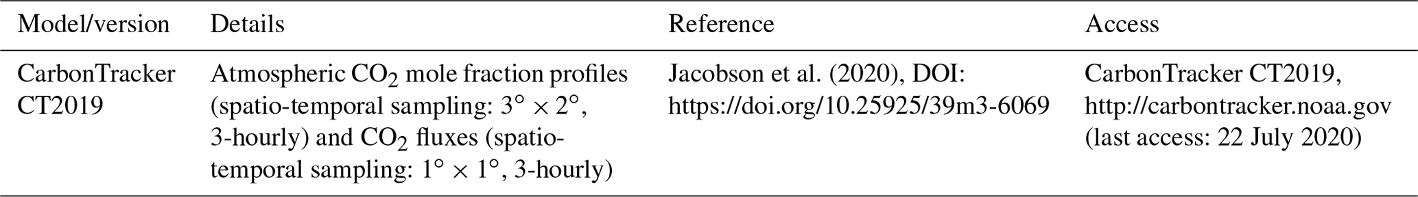
We use data from NOAA's (National Oceanic and Atmospheric Administration) CO₂ assimilation system, CarbonTracker (CT2019) (Jacobson et al., 2020; Peters et al., 2007), to define the relationship between XCO₂ anomalies and fossil fuel emissions. CarbonTracker is a global atmospheric inverse model that assimilates atmospheric CO₂ measurements to produce modelled fields of atmospheric CO₂ mole fractions by adjusting land biosphere and ocean CO₂ surface fluxes. An overview about CT2019 set is provided in Table 2, including references and access information. In short, CarbonTracker has a representation of atmospheric transport based on weather forecasts, as well as modules representing air–sea exchange of CO₂, photosynthesis and respiration by the terrestrial biosphere, and release of CO₂ to the atmosphere by fires and combustion of fossil fuels.

Table 2Overview of the CarbonTracker CT2019 data set. For this study we used data from the period January 2015 to December 2018.

Download Print Version | Download XLSX

3 Methods

3.1 Methods to compute XCO₂ anomalies (ΔXCO₂)

Satellite XCO₂ retrievals contain information on anthropogenic CO₂ emissions (e.g. Schneising et al., 2013; Reuter et al., 2014b, 2019; Nassar et al., 2017), but extracting this information requires appropriate data processing and analysis. For a strong (net) source region XCO₂ is typically higher compared to its surrounding area. Our method is based on computing and subtracting XCO₂ background values. The purpose of this background correction is to isolate the regional emission signal by removing large-scale spatial and day-to-day temporal XCO₂ variations, which cannot be dealt with in our simple data-driven method to estimate emissions.

XCO₂ varies temporally and spatially (e.g. Agustí-Panareda et al., 2019; Reuter et al., 2020; Gier et al., 2020), for example, due to quasi-regular uptake and release of CO₂ by the terrestrial biosphere, which results in a strong seasonal cycle, especially over northern mid- and high latitudes. Compared to fluctuations originating from the interaction of the terrestrial biosphere and the atmosphere, the spatio-temporal XCO₂ variations due to anthropogenic fossil fuel (FF) CO₂ emissions are typically much smaller (e.g. 1 ppm compared to 10 ppm; Schneising et al., 2008, 2013, 2014; Agustí-Panareda et al., 2019).

A method used for background correction is the one described in Hakkarainen et al. (2019; see also Hakkarainen et al., 2016, for a first publication of that method). We use two different methods for background correction. We refer to these methods as “daily anomalies via (latitude band) medians” (DAM), which is essentially identical with the method described in Hakkarainen et al. (2019), and “target minus surrounding” (TmS).

Hakkarainen et al. (2019) applied their method to the OCO-2 Level 2 XCO₂ data product to filter out trends and seasonal variations in order to isolate CO₂ source/sink signals. For background correction, Hakkarainen et al. (2019) calculate daily medians for 10^∘ latitude bands and linearly interpolate the resulting values to each OCO-2 data point. Instead of interpolation, we compute the median around each latitude (running median) using a latitude band width of ±15^∘. We use a larger width compared to Hakkarainen et al. (2019), as we also apply our method to GOSAT data, which are much sparser than OCO-2 data. Our investigations showed that the width of the latitude band is not critical. The band needs to be wide enough to contain a statistically significant sample but narrow enough to resolve large latitudinal gradients in CO₂. We subtract the corresponding median from each single XCO₂ observation in the original Level 2 XCO₂ data product files to obtain a data set of XCO₂ anomalies, ΔXCO $_{2}^{DAM}$ .

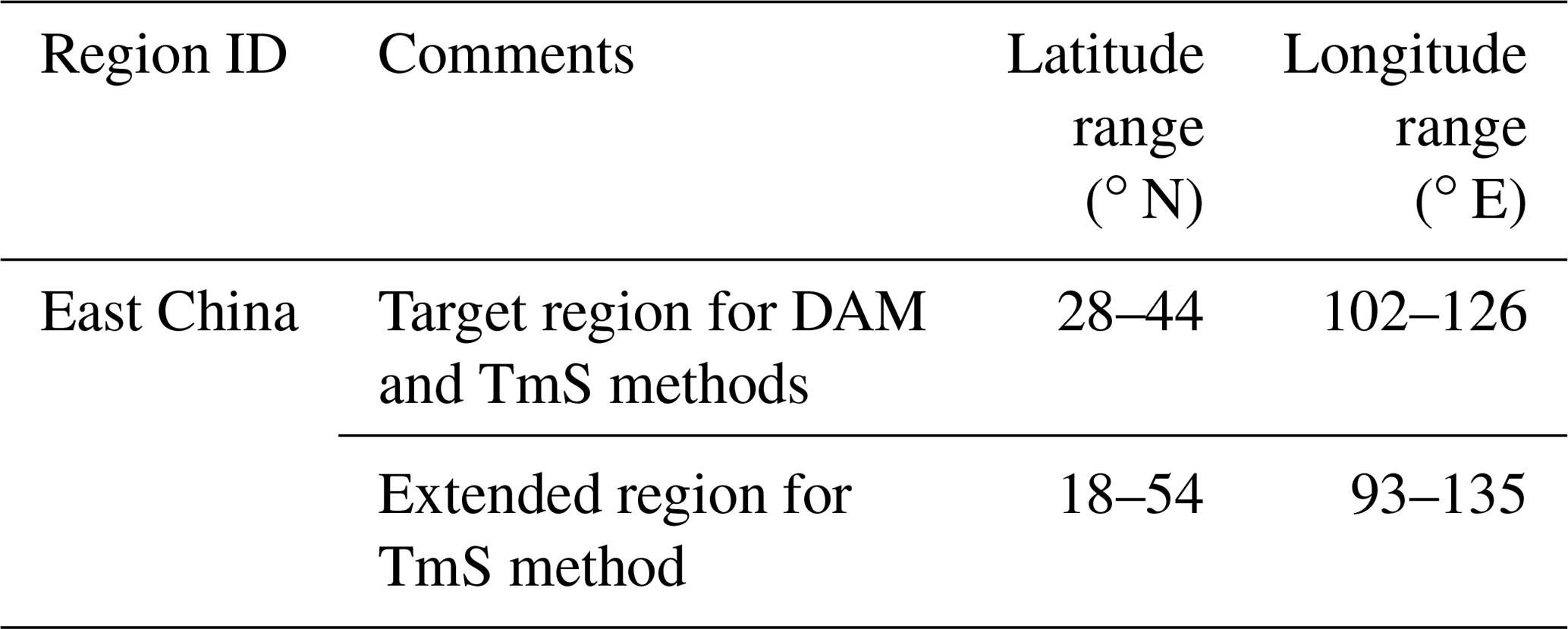
In order to verify that our results do not critically depend on the details of one method, we also use the second TmS method. Here we obtain the background by averaging XCO₂ in a region surrounding the target region (see Table 3 for the latitude and longitude corner coordinates of the target and its surrounding region).

Table 3Corner coordinates of the East China target region as analysed in this study.

Download Print Version | Download XLSX

We call these background-corrected XCO₂ retrievals XCO₂ anomalies, and satellite-derived maps and time series of these XCO₂ anomalies are presented and discussed in Sect. 4.1. These XCO₂ anomalies are then used to compute East China FF CO₂ emission estimates, CO $_{2}^{FF}$ , as described in the following subsection.

3.2 Computation of emission estimates (CO $_{2}^{FF}$ )

To determine whether satellite XCO₂ retrievals can provide information on relative changes of anthropogenic CO₂ emissions for the East China target region, we must establish a relationship between the XCO₂ anomalies (see Sect. 3.1) and the desired estimates of the target region fossil fuel (FF) emissions. To develop a method to convert the XCO₂ anomalies, ΔXCO₂, to FF emission estimates, CO $_{2}^{FF}$ , we use an existing model data set, the CarbonTracker CT2019 data set described in Sect. 2.2, which contains atmospheric CO₂ fields and corresponding CO₂ surface fluxes during 2015–2018.

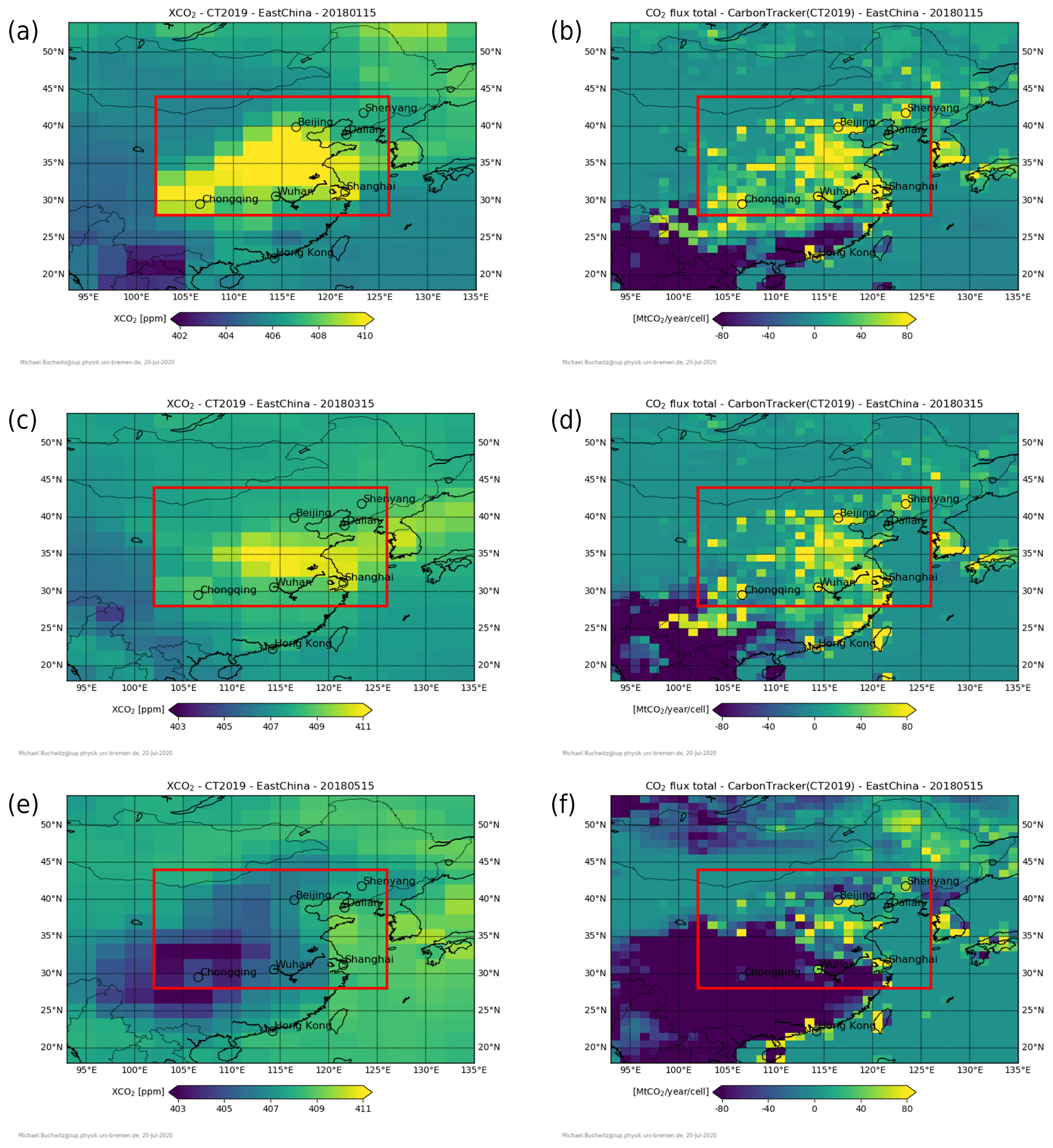
https://amt.copernicus.org/articles/14/2141/2021/amt-14-2141-2021-f01

Figure 1CT2019 XCO₂ (a, c, e, in ppm) and corresponding CO₂ surface fluxes (b, d, f, in Mt CO₂ yr⁻¹ per cell) for 15 January 2018 (a, b), 15 March 2018 (c, d) and 15 May 2018 (e, f). The red rectangle encloses the East China target region as defined for this study.

Figure 1 shows CT2019 XCO₂ maps (left) and corresponding surface CO₂ flux maps (right) for selected days in the January-to-May-2018 period. The XCO₂ has been computed by vertically integrating the CT2019 CO₂ vertical profiles (weighted with the surface pressure normalized pressure change over each layer). The model data are sampled at local noon, which is close to the overpass time of the satellite data sets used here. The spatio-temporal sampling of a specific satellite XCO₂ data product is not considered here; i.e. we use the CT2019 data set independent of any satellite data product apart for the sampling at local noon. As can be seen from Fig. 1, XCO₂ is clearly elevated over the East China target region (red rectangle) relative to its surrounding region on 15 January 2018 (Fig. 1a) and on 15 March 2018 (Fig. 1c). On 15 May 2018 (Fig. 1e) the target region and parts of the surrounding region contain large areas of lower-than-average XCO₂, a pattern which primarily results from carbon uptake by vegetation during the growing season, which starts in eastern China around May each year. The CO₂ fluxes, which are shown on the right-hand side panels of Fig. 1, show similar spatial pattern as the XCO₂ maps, but due to atmospheric transport and the long lifetime of atmospheric CO₂ there is no one-to-one correspondence between atmospheric XCO₂ and surface emissions. The CO₂ fluxes are the sum of several contributing fluxes including FF emissions, biogenic fluxes and other fluxes (fires, oceans).

https://amt.copernicus.org/articles/14/2141/2021/amt-14-2141-2021-f02

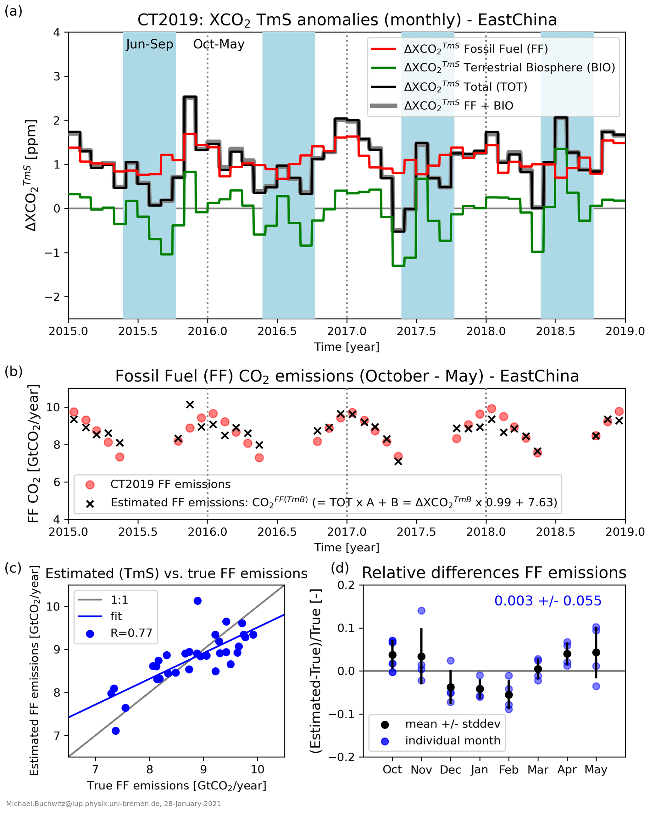
Figure 2Results obtained by applying the DAM method to CT2019 XCO₂ for East China. (a) Different monthly ΔXCO $_{2}^{DAM}$ components: total ΔXCO $_{2}^{DAM}$ (TOT) and its FF (red) and biogenic (BIO, green) components and their sum (FF + BIO). The non-shaded time periods October to May indicate the periods analysed in this publication. (b) East China October-to-May FF CO₂ emissions (red dots) and estimated emissions CO $_{2}^{FF (DAM)}$ (black crosses) as obtained from total ΔXCO $_{2}^{DAM}$ (TOT as shown in panel a) using the formula shown in panel (b). (c) Scatter plot of estimated versus true (i.e. CT2019) FF emissions. (d) Relative difference of estimated and true emissions.

Download

Figure 2a shows time series obtained by applying the DAM method to CT2019 XCO₂ for the East China target region. The CT2019 data set not only contains atmospheric CO₂ concentrations but also its components due to fossil fuel (FF) emissions and biogenic (BIO) and other fluxes. From the CT2019 data set we computed total XCO₂ (TOT) and its FF and BIO components. From these components we subtracted the background using the DAM method, and the corresponding monthly ΔXCO $_{2}^{DAM}$ time series are shown in Fig. 2a. As can be seen from Fig. 2a, total ΔXCO $_{2}^{DAM}$ (black line) is dominated by its FF (red line) and BIO (green line) components (their sum, i.e. FF + BIO (grey line), is close to TOT (black line)). As can also be seen, FF emissions for East China (red line) are larger than the BIO fluxes (green line) at least during October to April. During May to September the BIO fluxes are negative due to uptake of atmospheric CO₂ by the terrestrial biosphere, and their absolute value is on the same order or may even significantly exceed the FF emissions. As a consequence, total ΔXCO $_{2}^{DAM}$ (black line) gets negative. During these months, the total anomaly (black line) is closer to BIO (green line) than to FF (red line).

The task for the satellite inversion is to obtain estimates of East China FF CO₂ emissions from the satellite-derived (total) XCO₂ anomalies, ΔXCO $_{2}^{DAM}$ (black line in Fig. 2a). To determine to what extent this is possible, we fitted CT2019 ΔXCO $_{2}^{DAM}$ (i.e. the quantity that we can also obtain from satellites) to the East China CT2019 FF CO₂ emissions (which are the known true emissions in this model data assessment exercise). The results are shown in Fig. 2b for October-to-May periods. The estimated emissions (black crosses) have been obtained via a linear fit of ΔXCO $_{2}^{DAM}$ to the CT2019 FF emissions (red dots). The two parameters of the linear fit are also shown in Fig. 2b: scaling factor A (= 0.90) and offset B (= 7.41). As can be seen, the estimated emissions agree reasonably well with the true emissions. The linear correlation coefficient R is 0.83 (see Fig. 2c), and the relative difference in terms of mean and standard deviation is 0.2 % ± 5 % (see Fig. 2d). However, for individual months the error can be as large as 10 %. From this we conclude that the (approximately 2σ) uncertainty of our method is approximately 10 %.

A similar figure but generated using the TmS method is shown in Appendix A as Fig. A1. As can be seen, the results shown in Fig. A1b to d are similar to the ones shown in Fig. 2b to d, but the linear correlation is slightly worse and the errors are slightly larger. In contrast, the time series shown in panel (a) differ significantly. This is because of the different background corrections used for the two methods. But despite these significant differences the quality of the derived emissions is similar (the standard deviation of the monthly biases is 5.5 % for TmS and 4.8 % for DAM; see panel d). Nevertheless, the DAM method gives slightly better results compared to the TmS method, and this is also confirmed by applying both methods to the satellite data (see Sect. 4). Therefore, the DAM method is our baseline method, and we focus on results obtained with the DAM method.

It is perhaps surprising that the offset (fit parameter B; see above) is so large (7.41 for DAM and 7.63 for TmS). Probably one would assume that the XCO₂ anomalies ΔXCO₂ are directly proportional to the target region fossil fuel emissions, i.e. one would assume that FF is (approximately) equal to a constant multiplied by ΔXCO₂ (no offset added) (for example, for FF = 8 Gt CO₂ yr⁻¹ and ΔXCO₂ = 2 ppm one would have expected that the conversion factor is 4 Gt CO₂ yr⁻¹ ppm⁻¹). In that case, as we are only interested in relative changes in emissions, we would not need to know the exact value of the scaling factor. However, when analysing the satellite data, we found that ΔXCO₂ is around 2 ppm for January but decreases in subsequent months, nearly approaching zero in May (which is consistent with the CT2019 results shown in Fig. 2a). As anthropogenic emissions are not expected to change that much within a few months (and zero emissions around May are not realistic at all), we concluded that the simple proportionality assumption does not hold. To investigate this we used the CT2019 data set to test and improve our method, and the results are reported in this section. We applied our method to CT2019 XCO₂ (as shown in Fig. 2) and compared the retrieved FF values with the (true) CT2019 FF values. We found large differences, which could be significantly reduced by adding an offset to the linear fit as discussed above. The reason for the large offset is the influence of the biosphere. Around May the uptake of atmospheric CO₂ due to the biosphere is so large that ΔXCO₂ is close to zero – but the FF emissions are not – and the East China target region is essentially carbon neutral or even a net sink (see also Fig. 1).

As explained, scaling factor A and offset B are obtained empirically via a linear fit using CT2019 data (Fig. 2b) and used for the conversion of the satellite XCO₂ anomalies during the entire time period January 2015 to May 2020 (as will be shown in Sect. 4). As can be seen from Fig. 2b and c, the retrieval biases are within ±10 % during 2015–2018. We assume in our study that the same conversion is also appropriate for 2019 and 2020. However, it cannot be ruled out that 2019 or 2020 were significantly different compared to previous years with respect to aspects relevant for our study. To address this, we compare the period October 2019 to May 2020 results with the corresponding results from previous October-to-December periods to find out to what extent the period of interest, i.e. October 2019 to May 2020, is significantly different, taking into account the year-to-year variability, which we use to obtain uncertainty estimates.

The methods described in this section have been applied to convert satellite-derived target region XCO₂ anomalies, ΔXCO₂, into estimated target region FF CO₂ emissions, CO $_{2}^{FF}$ . How this has been done using the DAM method for background correction is explained in the following Sect. 4, where we refer for the corresponding TmS method results to Appendix A.

4 Results and discussion

In this section, we present results obtained by applying the DAM method (see Methods Sect. 3.1) to the satellite data to obtain XCO₂ anomalies from which we derive FF emission estimates (see Methods Sect. 3.2).

4.1 Application of the DAM method to satellite XCO₂ retrievals

The DAM method has been applied to the OCO-2 and GOSAT satellite XCO₂ data products listed in Table 1. Figure 3 shows a global OCO-2 DAM XCO₂ anomaly map at 1^∘ × 1^∘ resolution for the period 2015–2019. A similar map is shown in Hakkarainen et al. (2019; see their Fig. 3, top panel). The degree of agreement confirms the finding reported in Sect. 3.1 that the generation of these anomaly maps does not critically depend on how exactly the median is computed and used to subtract the background. Hakkarainen et al. (2019) discuss their OCO-2-derived maps in quite some detail also in terms of seasonal averages and comparisons with model simulations. They show that positive anomalies correspond to fossil fuel combustion over major industrial areas including China. Their seasonal maps (see their Fig. 4) show a strong positive anomaly over East China (similar to that shown here in Fig. 3) except for the June–August (JJA) summer season, where the XCO₂ anomaly can be negative. This is consistent with the CT2019 results presented in Sect. 3.2.

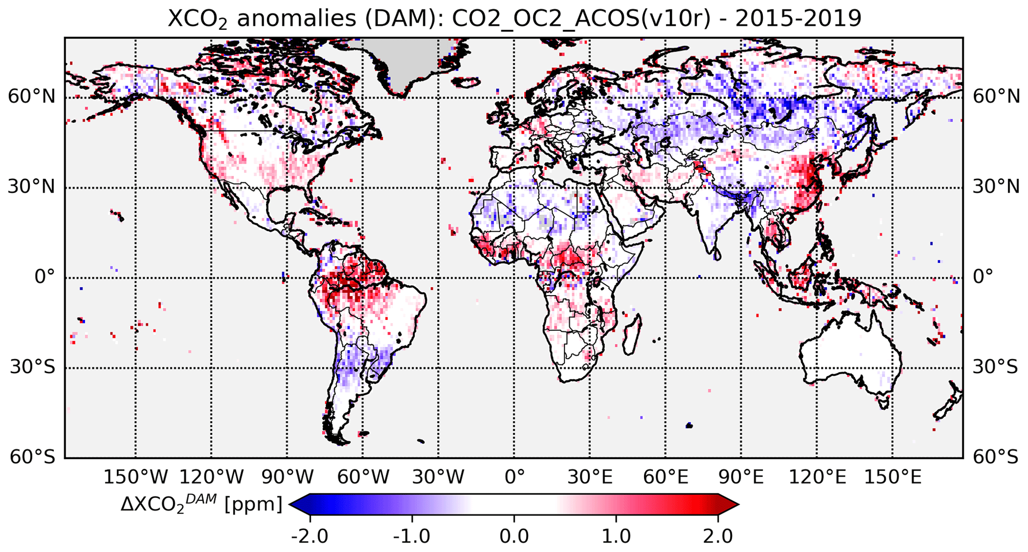
https://amt.copernicus.org/articles/14/2141/2021/amt-14-2141-2021-f03

Figure 3DAM XCO₂ anomaly map at 1^∘ × 1^∘ resolution generated from OCO-2 Level 2 XCO₂ (v10r, land) for 2015 to 2019.

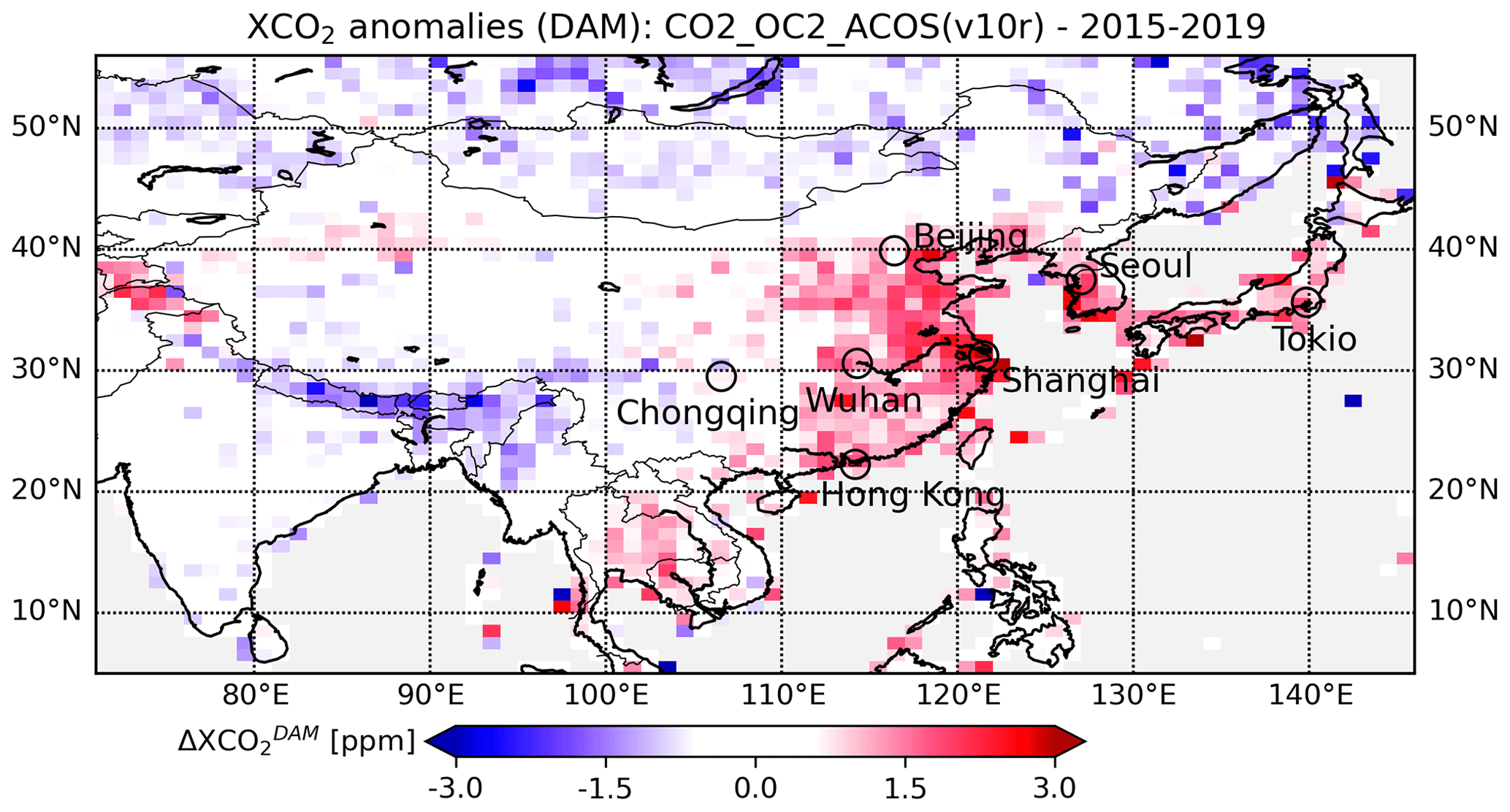
https://amt.copernicus.org/articles/14/2141/2021/amt-14-2141-2021-f04

Figure 4As Fig. 3 but for China and surrounding areas.

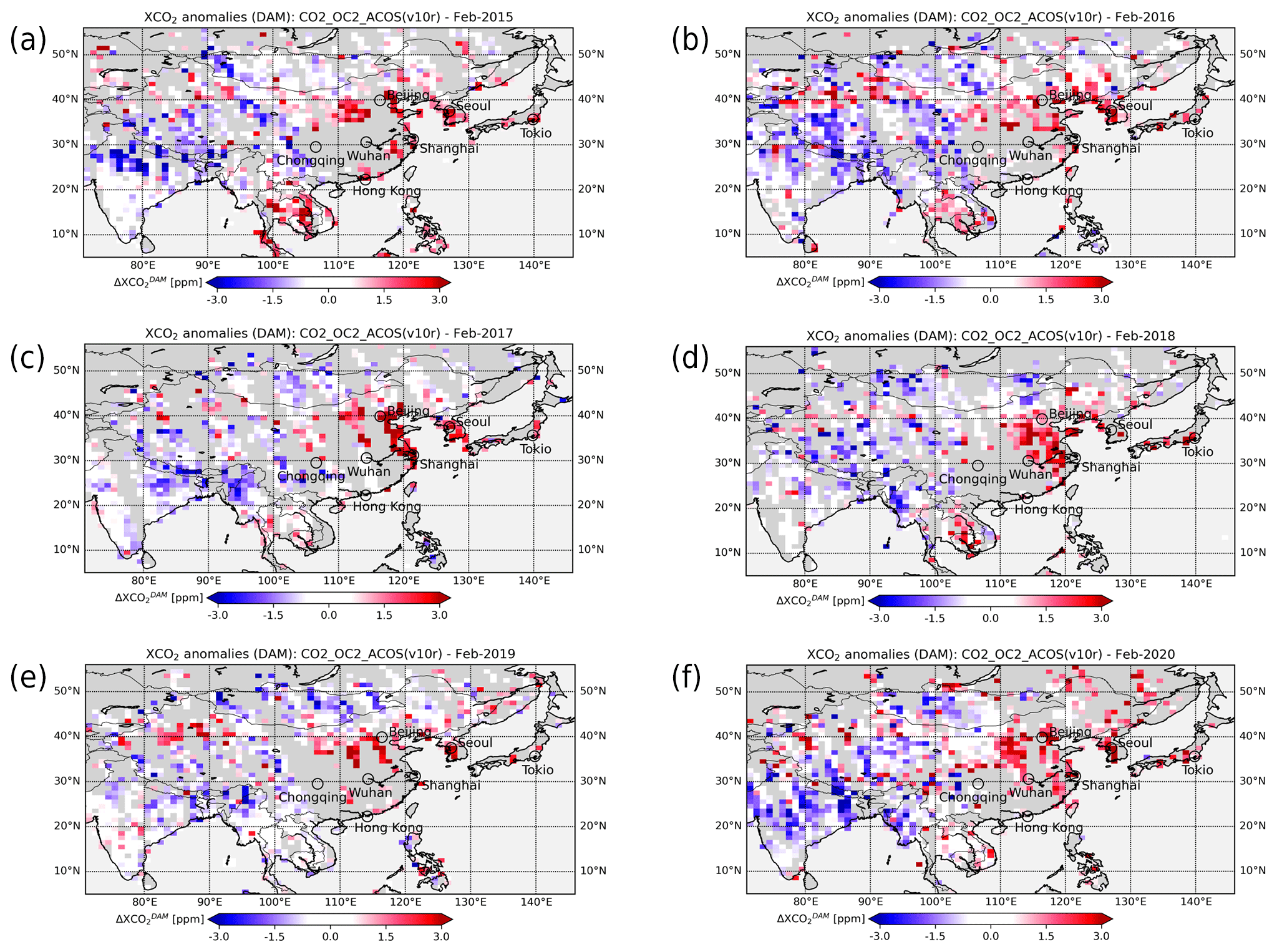
https://amt.copernicus.org/articles/14/2141/2021/amt-14-2141-2021-f05

Figure 5As Fig. 4 but for (a) February 2015 to (f) February 2020.

A zoom into Fig. 3 is presented in Fig. 4, which shows more details for China and its surrounding area. As can be seen from Fig. 4, ΔXCO $_{2}^{DAM}$ is positive especially in the region between Beijing, Wuhan and Hong Kong, with the highest values in the area between Beijing and Shanghai. This positive anomaly indicates that this region is a strong CO₂ source region as also discussed in Hakkarainen et al. (2019). As already explained, there is no one-to-one correspondence (especially not for every grid cell) between local XCO₂ anomalies and local CO₂ emissions (or uptake) because the emitted CO₂ is transported and mixed in the atmosphere. Furthermore, the satellite data are typically sparse due to strict quality filtering to avoid potential XCO₂ biases, for example, due to the presence of clouds. Cloud-contaminated ground scenes are identified to the extent possible via the corresponding retrieval algorithm (see references listed in Table 1) and flagged to be bad and are therefore not used for this analysis. The sparseness of the satellite data set is obvious from Fig. 5, which shows OCO-2 DAM XCO₂ anomaly maps for February during the 6 years 2015 to 2020.

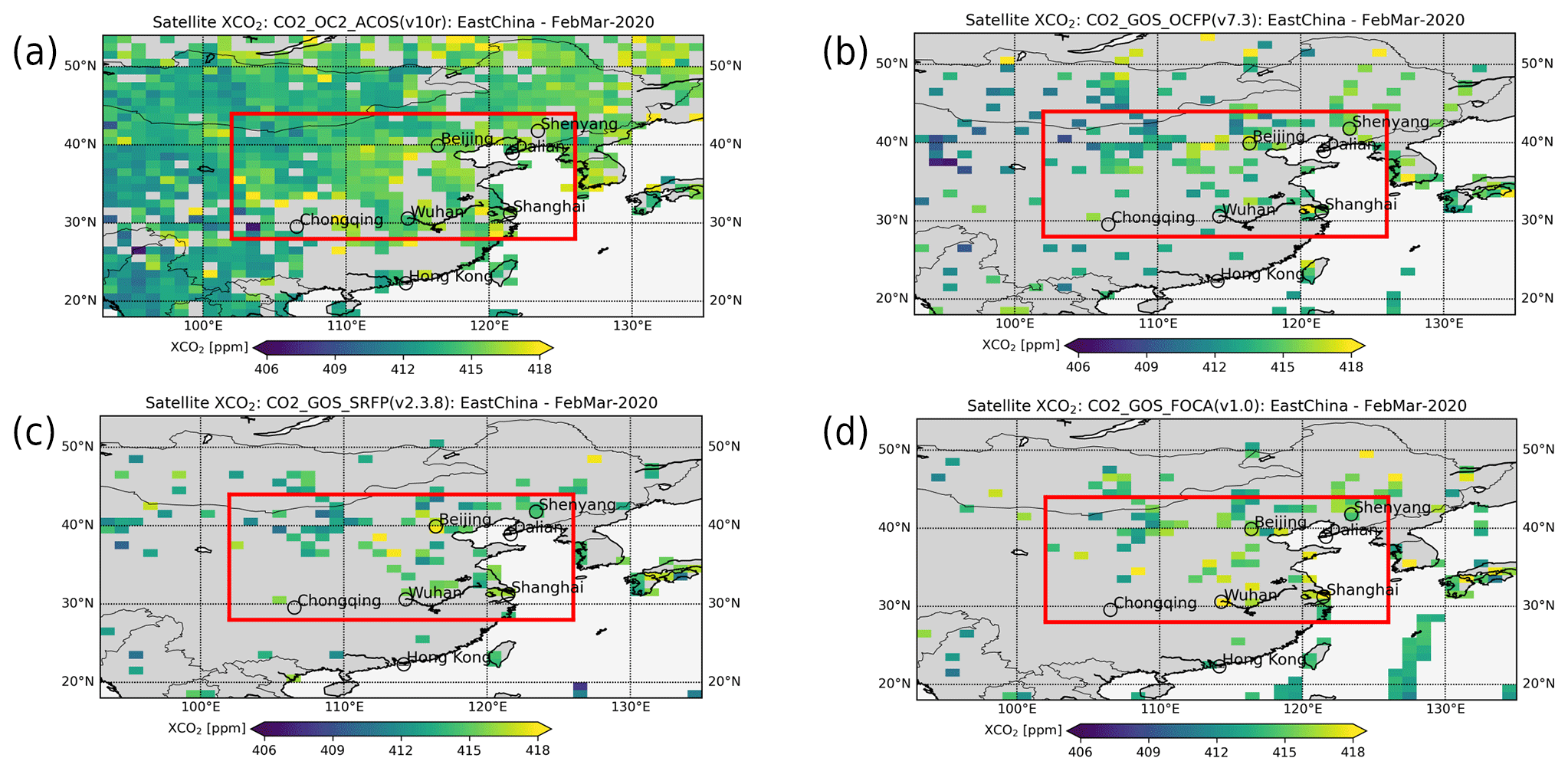
https://amt.copernicus.org/articles/14/2141/2021/amt-14-2141-2021-f06

Figure 6(a) OCO-2 XCO₂ (version 10r, product ID CO2_OC2_ACOS) over land at 1^∘ × 1^∘ resolution for February–March 2020. The red rectangle encloses the investigated East China target region. (b–d) As panel (a) but for products CO2_GOS_OCFP (b), CO2_GOS_SRFP (c) and CO2_GOS_FOCA (d) (see Table 1 for details).

A key difference between the OCO-2 and the GOSAT data products is the different sampling of the target region, with GOSAT having much sparser coverage compared to OCO-2. This is illustrated in Fig. 6, which shows February-to-March-2020 averages of the OCO-2 XCO₂ data product (Fig. 6a) and the three GOSAT data products (Fig. 6b–d) at 1^∘ × 1^∘ resolution. The OCO-2 product shown in Fig. 6a is NASA's OCO-2 operational Atmospheric CO₂ Observations from Space (ACOS) algorithm version 10r bias-corrected XCO₂ product (the so-called Lite product), which is referred to in this publication via the product identifier (ID) CO2_OC2_ACOS. The three GOSAT XCO₂ products are (see details and references as given in Table 1) the University of Leicester's GOSAT product (ID CO2_GOS_OCFP; Fig. 6b), SRON Netherlands Institute for Space Research GOSAT product (CO2_GOS_SRFP; Fig. 6c), and University of Bremen's GOSAT product (CO2_GOS_FOCA; Fig. 6d) as retrieved with the Fast atmOspheric traCe gAs retrievaL (FOCAL) retrieval algorithm initially developed for OCO-2 (Reuter et al., 2017a, b). As can be seen from Fig. 6, the spatial sampling of the target region is different for each product as only quality-filtered (i.e. good) data are shown and the quality filtering is algorithm specific (see references listed in Table 1).

Figure 6 also shows as red rectangle the East China target region as defined for this study (the geographical coordinates are listed in Table 3). The fossil fuel (FF) CO₂ emissions of this target region are approximately 8 Gt CO₂ yr⁻¹; i.e. the selected target region covers approximately 80 % of the FF emissions of all of China, which are approximately 10 Gt CO₂ yr⁻¹ (Le Quéré et al., 2018; Friedlingstein et al., 2019). In the following section we present East China FF emission estimates as derived from the satellite XCO₂ anomalies during and before the COVID-19 period.

4.2 Emission estimates

Carbon dioxide fossil fuel emission estimates, CO $_{2}^{FF}$ , have been derived from the XCO₂ anomalies, ΔXCO₂, computed for each of the four satellite XCO₂ data products listed in Table 1. In this section the emission results are presented and discussed. We focus on results based on ΔXCO₂ derived with the DAM method and refer to Appendix A for results based on the TmS method.

4.2.1 Emission estimates from NASA's OCO-2 (version 10r) XCO₂

Figure 7 shows the results obtained by applying the DAM method to product CO2_OC2_ACOS (see Table 1) for the East China target region for the period January 2015 to May 2020 (the TmS version of this figure is shown as Fig. A2 in Appendix A). Figure 7a shows daily DAM XCO₂ anomalies as a thin grey line and the corresponding monthly averages as red dots. The amplitude (approximately ±1 ppm) and time dependence (e.g. the minimum in the middle of each year) are similar to that for CT2019 (Fig. 2a black line). To ensure that there are a sufficiently large number of observations per month, two criteria need to be fulfilled: There must be a minimum number of days per month (here: 5) and a minimum number observations per day (here: 30). The latter criterion is also relevant for the daily data shown in Fig. 7(a) (grey line). We also used other combinations of these two parameters (as shown below, e.g. Fig. 9).

https://amt.copernicus.org/articles/14/2141/2021/amt-14-2141-2021-f07

Figure 7DAM analysis of the OCO-2 ACOS version 10r XCO₂ product (CO2_OC2_ACOS) for the East China region from January 2015 to May 2020. (a) The thin grey line shows the daily DAM XCO₂ anomalies, i.e. daily ΔXCO $_{2}^{DAM}$ . The red dots are the corresponding monthly values, which are also shown in panel (b) for different October–May periods. (c) As panel (b) but for CO $_{2}^{FF (DAM)}$ , i.e. for the estimated East China monthly FF emissions (see main text). The data for October 2019–May 2020 (10.2019–5.2020) are shown in red (see annotation for other periods). (d) Relative CO $_{2}^{FF (DAM)}$ differences for different periods. In blue, for example, the differences correspond to the period 10.2019–5.2020 (shown in red in panel c) minus 10.2018–5.2019 (shown in blue in panel c). (e) As panel (d) but after the October-to-December mean value (OND anomalies). The following parameters have been used to generate this figure: minimum number of observations per day: 30; minimum number of days per month: 5.

Download

Figure 7b shows monthly ΔXCO $_{2}^{DAM}$ for different October-to-May periods, and Fig. 7c shows the corresponding estimated FF emissions, CO $_{2}^{FF (DAM)}$ . Figure 7d shows relative differences of the time series shown in Fig. 7c. For example, the blue data are referred to as “(2020–2019)/2019” in Fig. 7d, where 2019 refers to the blue data in Fig. 7c, which corresponds to the period ending in May 2019. Shown are differences of year 2020 data (red in Fig. 7c) minus data from previous periods; i.e. Fig. 7d shows to what extent 2020 (strictly speaking the period October 2019–May 2020, i.e. the period which ends in 2020) differs relative to previous October-to-May periods.

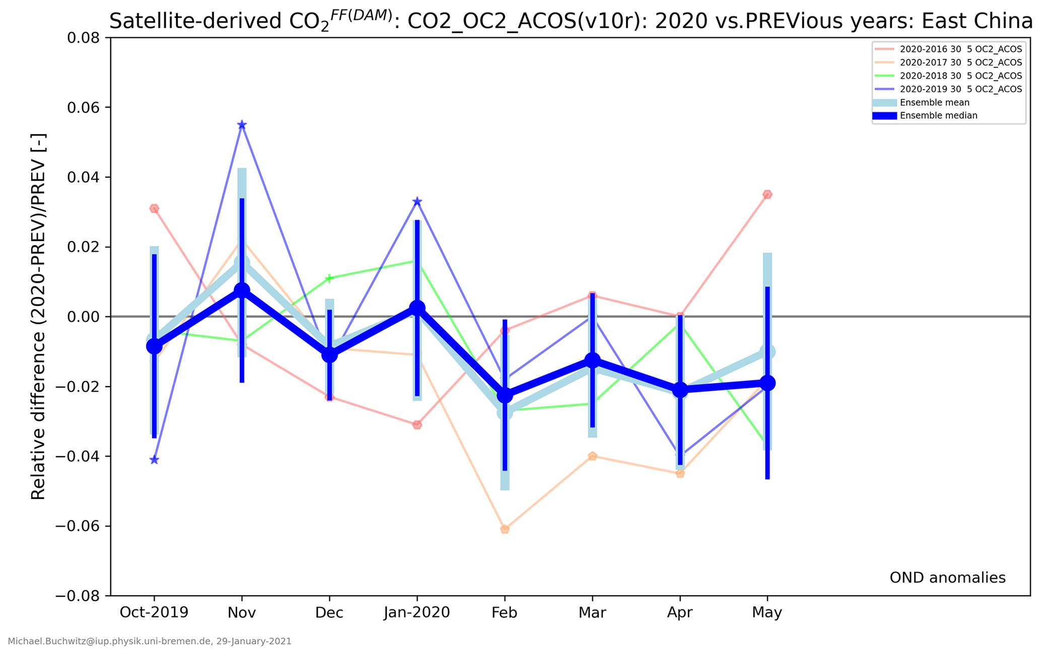
https://amt.copernicus.org/articles/14/2141/2021/amt-14-2141-2021-f08

Figure 8Ensemble member CO $_{2}^{FF (DAM)}$ OND anomalies derived from the satellite product CO2_OC2_ACOS. The thin lines and small symbols show the same data also shown in the bottom panel of Fig. 7. The thick dots and lines show the corresponding ensemble median, mean and scatter. The following parameters have been used to generate this figure (see also annotation): minimum number of observations per day: 30; minimum number of days per month: 5.

Download

To find out if we can detect a difference between the COVID-19 period and pre-COVID-19 periods, we subtract from each time series shown in Fig. 7d the October-to-December (OND) mean value. The corresponding time series are shown in Fig. 7e and are referred to as OND anomalies in the following. As can be seen from Fig. 7e, the OND anomalies vary within ±5 %. Values before January scatter around zero as the mean value of OND anomalies is zero by definition during October to December. In January the values also scatter around zero. After January most values are negative, indicating reduced emissions compared to pre-COVID-19 periods. This can be seen more clearly in Fig. 8, where the same data as in Fig. 7e are shown, but in addition the ensemble mean (light blue thick lines and dots) and median (royal blue thick lines and dots) has been added, including uncertainty estimates as computed from the standard deviation of the ensemble members.

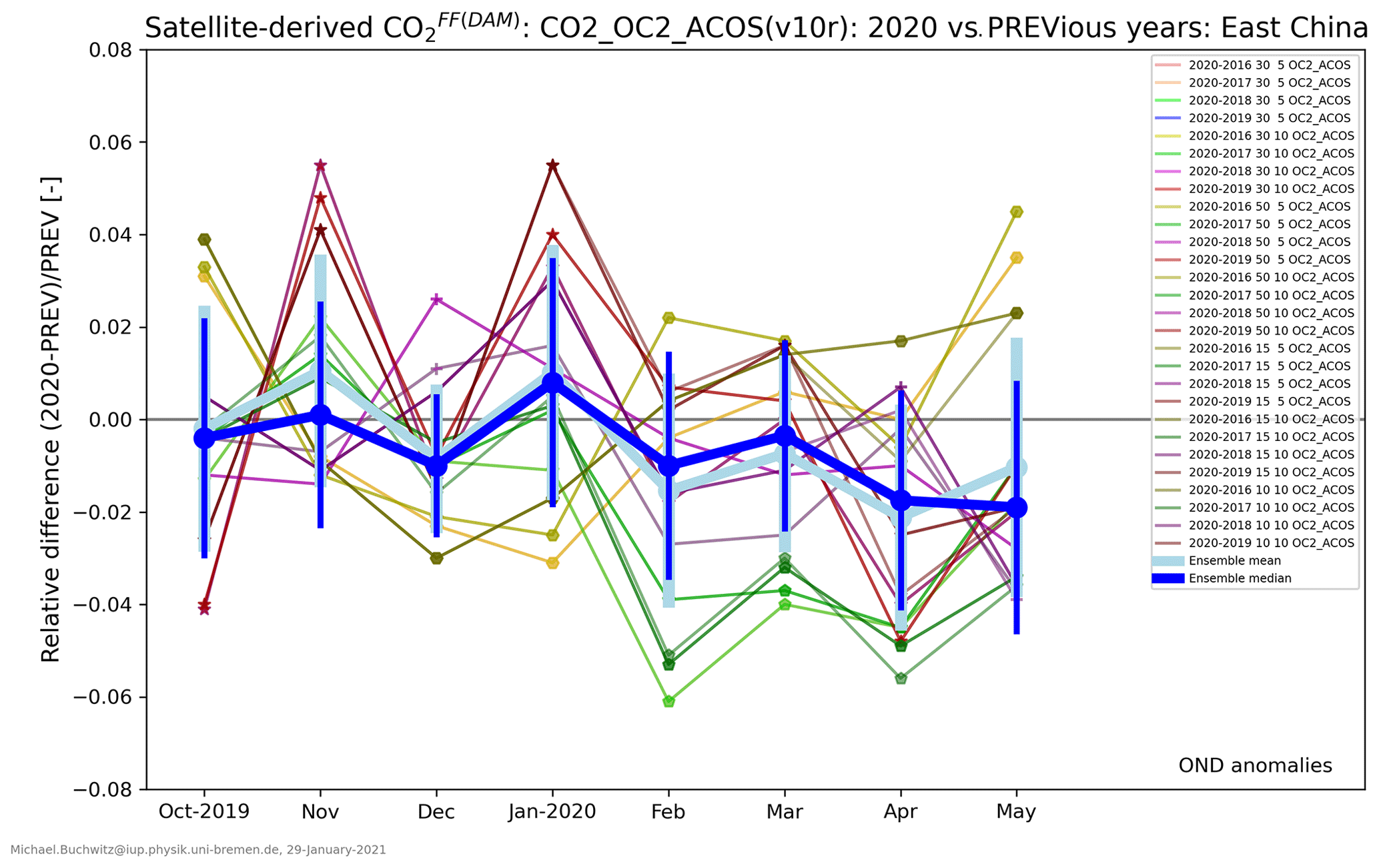
https://amt.copernicus.org/articles/14/2141/2021/amt-14-2141-2021-f09

Figure 9The same as Fig. 8 but with additional combinations of minimum number of observations per day (30 as in Fig. 8 and in addition 50, 15 and 10) and minimum number of days per month (5 as in Fig. 8 and in addition 10) (see annotation).

Download

Figures 7 and 8 have been generated with the requirement that for each day at least 30 observations need to be available in the target region and for each month at least 5 d fulfilling this 30 observations per day requirement. Figure 9 is similar to Fig. 8 except that also results for additional combinations have been added, i.e. other combinations of minimum number of observations per day and minimum number of days per month. As can be seen, the results depend somewhat on which combination of these parameters is used, but the ensemble median and its uncertainty (royal blue symbols and lines) are similar. The ensemble median values are similar and negative during February to May 2020. The large uncertainties (vertical lines; 1σ error estimates) reflect the scatter of the ensemble members. The errors bars (1σ) overlap with the zero (i.e. no reduction) line, indicating that it cannot be claimed with confidence that a significant drop of the emissions during the COVID-19 period has been detected.

4.2.2 Emission estimates from GOSAT XCO₂ data products

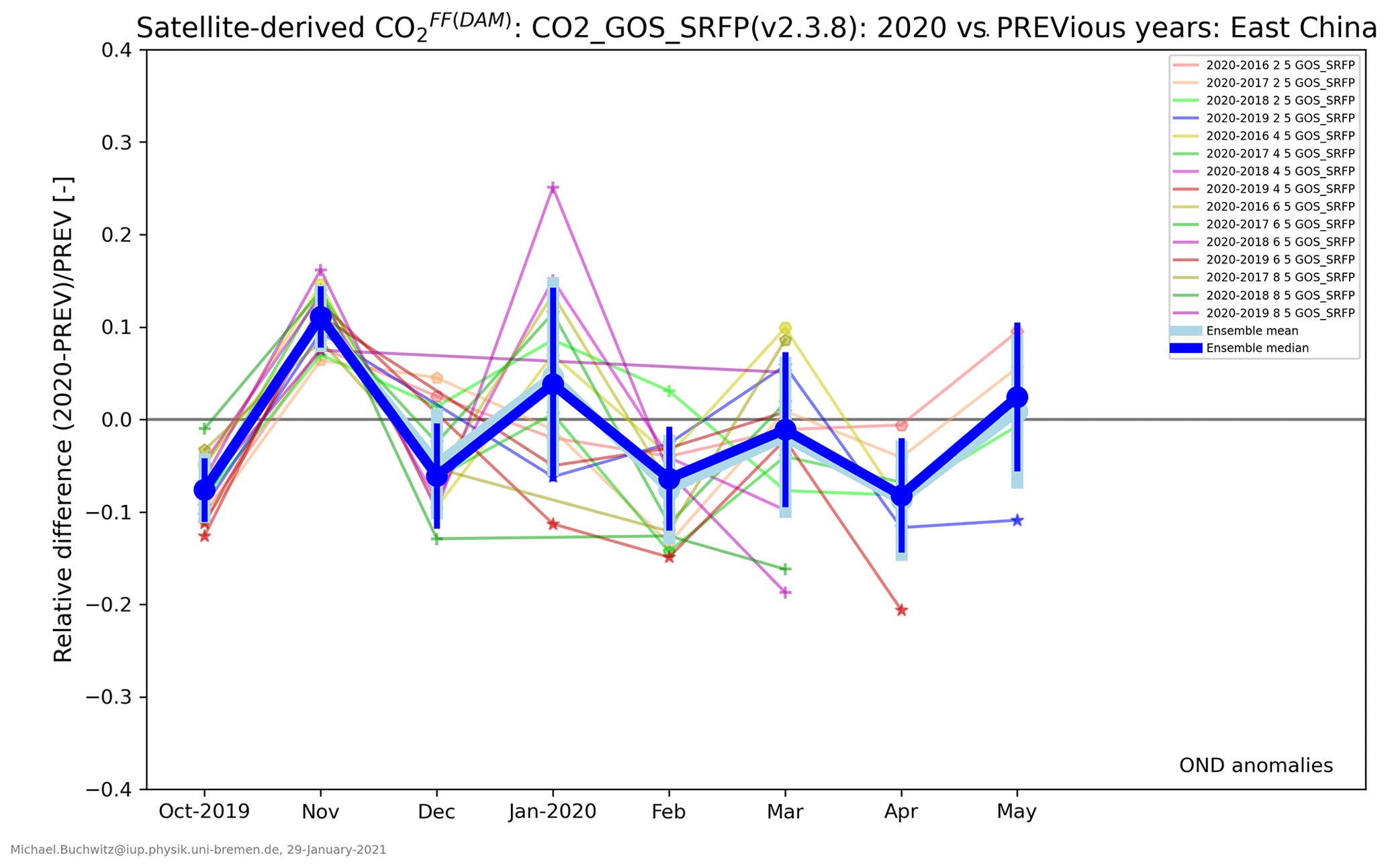
The same analysis method as applied to NASA's OCO-2 data product (Sect. 4.2.1) has also been applied to the three GOSAT XCO₂ data products listed in Table 1. The results are shown in Fig. 10 for product CO2_GOS_OCFP, in Fig. 11 for product CO2_GOS_SRFP and in Fig. 12 for product CO2_GOS_FOCA. The month-to-month variations are larger for these GOSAT products compared to OCO-2 product (note the different scale of the y axes compared to Fig. 9). This is because GOSAT products are much sparser compared to the OCO-2 product (as shown in Fig. 6) and because the single observation random error is larger for GOSAT compared to OCO-2. As can be seen from a comparison of the results obtained for the three GOSAT products (Figs. 10–12), there are large differences among the results obtained from these products. For example, product CO2_GOS_OCFP (Fig. 10) suggests that the largest emission reduction is in April, in contrast to the other two products. The large spread of the GOSAT results means that no clear conclusions can be drawn concerning East China emission reductions during the COVID-19 period.

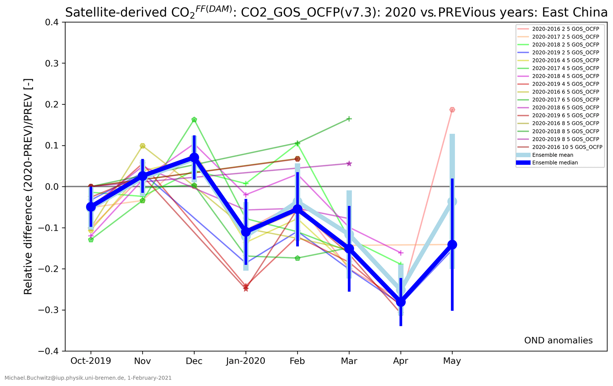
https://amt.copernicus.org/articles/14/2141/2021/amt-14-2141-2021-f10

Figure 10The same as Fig. 9 but for the product CO2_GOS_OCFP. Results are shown for several values of the required minimum number of observations per day: 2, 4, 6, 8, 10 and 15. The required minimum number of days per month is 5.

Download

https://amt.copernicus.org/articles/14/2141/2021/amt-14-2141-2021-f11

Figure 11The same as Fig. 10 but for the product CO2_GOS_SRFP.

Download

https://amt.copernicus.org/articles/14/2141/2021/amt-14-2141-2021-f12

Figure 12The same as Fig. 10 but for the product CO2_GOS_FOCA.

Download

4.2.3 Ensemble mean and uncertainty

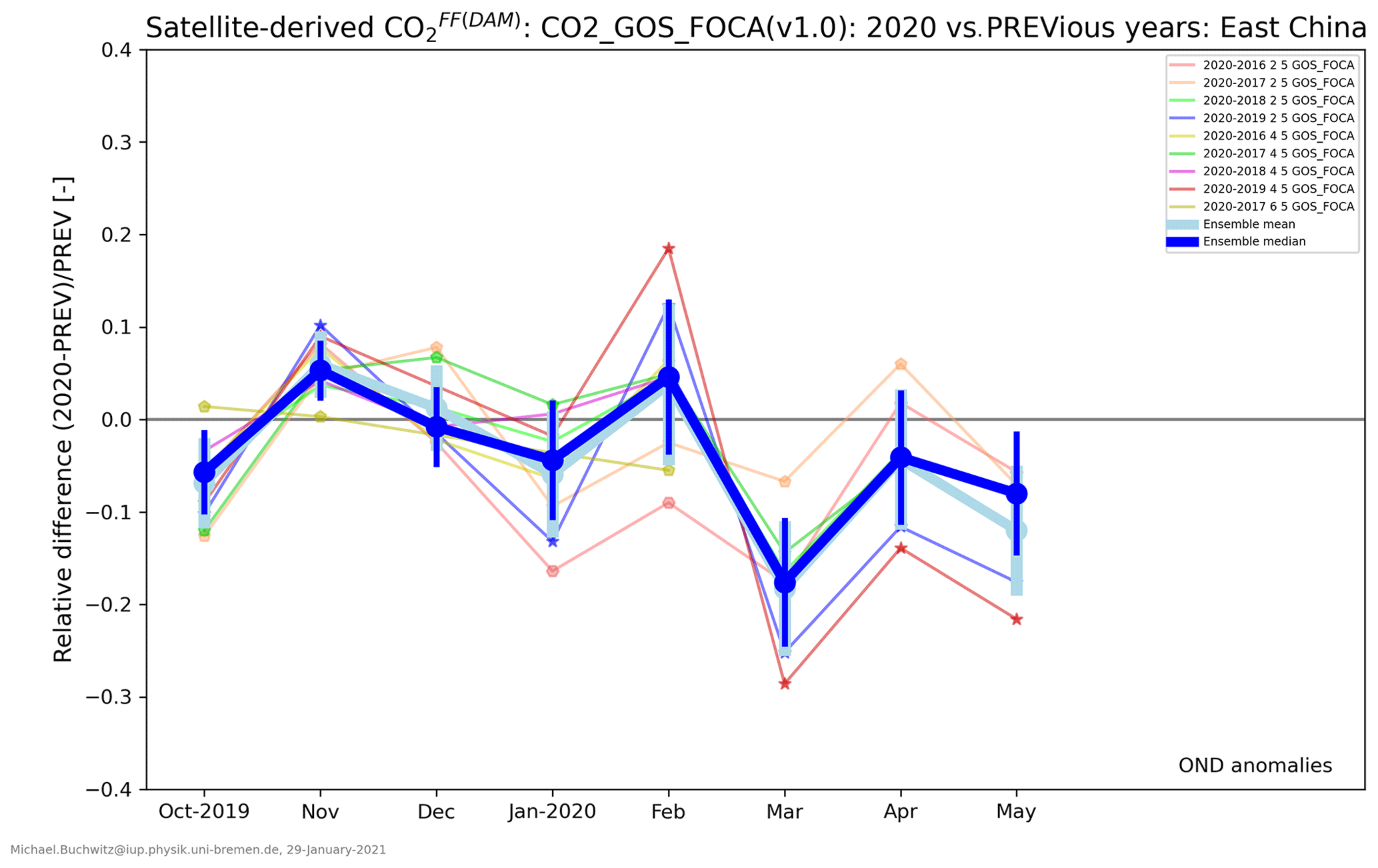
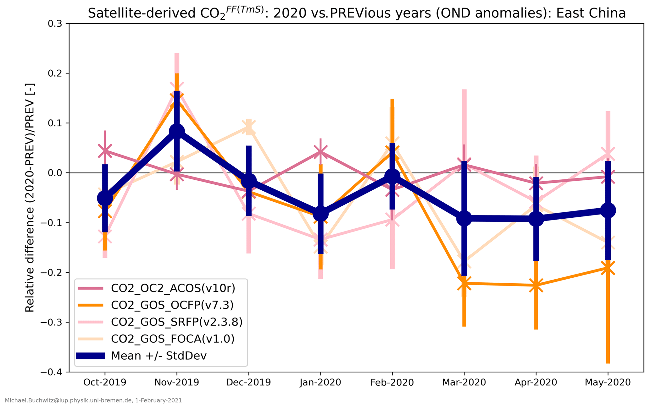
An overview about the results obtained from all four satellite data products using the DAM method is shown in Fig. 13 (the corresponding TmS version of this figure is shown as Fig. A3 in Appendix A). The results obtained from the individual products (as shown in royal blue in Figs. 9–12) are shown here using reddish colours (the corresponding numerical values are listed in Table 4). Also shown in Fig. 13 is the mean of the ensemble members and its estimated uncertainty (in dark blue); the corresponding numerical values are listed in the bottom row of Table 4. The ensemble mean suggests emission reductions by approximately 10 % ± 10 % in March and April 2020. However, as can also be seen, there are significant differences across the ensemble of satellite data products. For example, the analysis of the OCO-2 data suggests a much smaller emission reduction of only about 1 %–2 %. Because of the large differences between the individual ensemble members it is concluded that the expected emission reduction cannot be reliably detected and accurately quantified with our method.

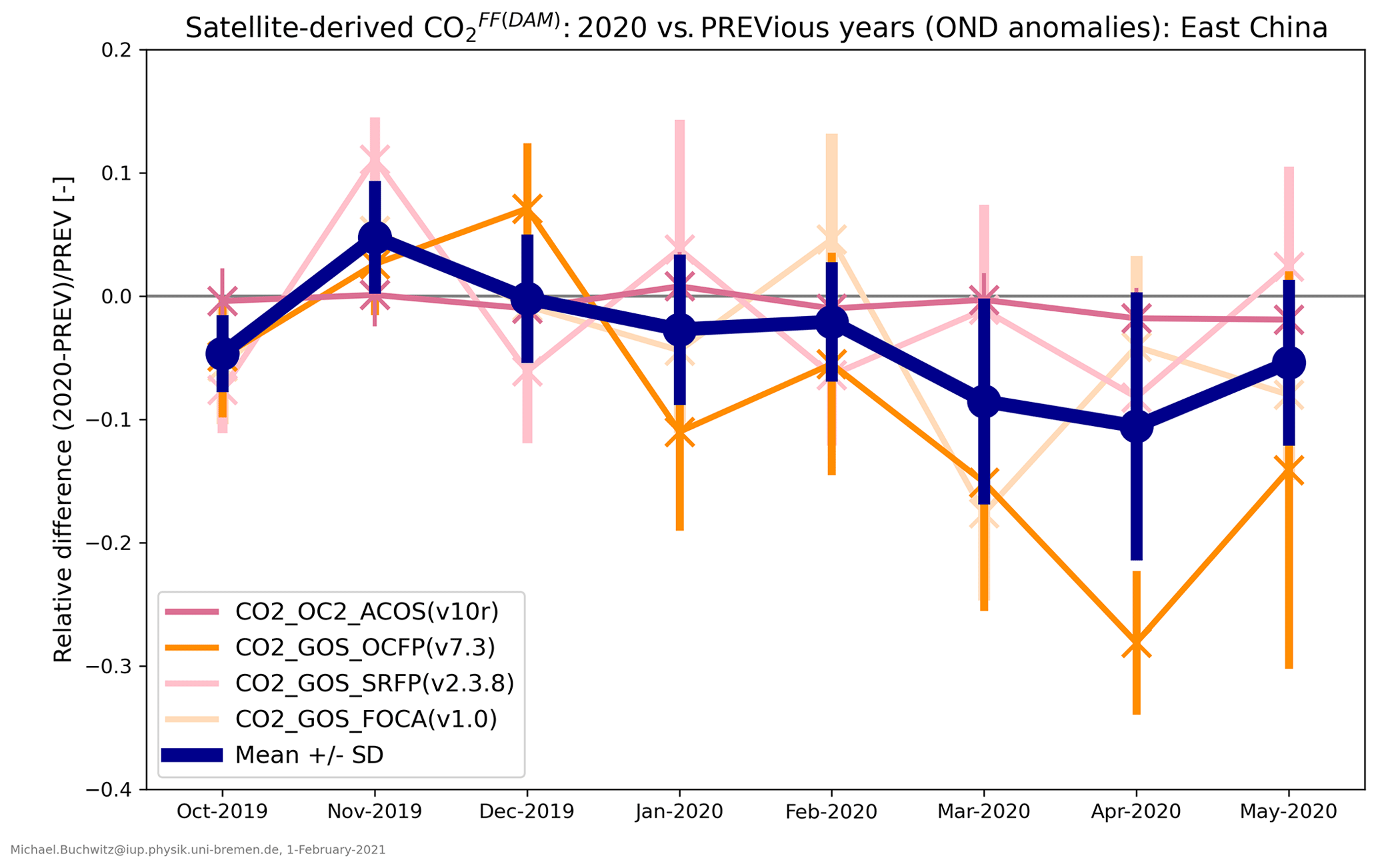
https://amt.copernicus.org/articles/14/2141/2021/amt-14-2141-2021-f13

Figure 13Overview of the ensemble-based CO $_{2}^{FF (DAM)}$ results for January–May 2020 relative to October–December 2019 and previous years (also shown in Figs. 9–12) via reddish colours for each of the four analysed satellite XCO₂ data products (see Table 1). The corresponding ensemble mean value and its uncertainty is shown in dark blue. The uncertainty has been computed as the standard deviation of the ensemble members. The corresponding numerical values of the ensemble members are listed in Table 4.

Download

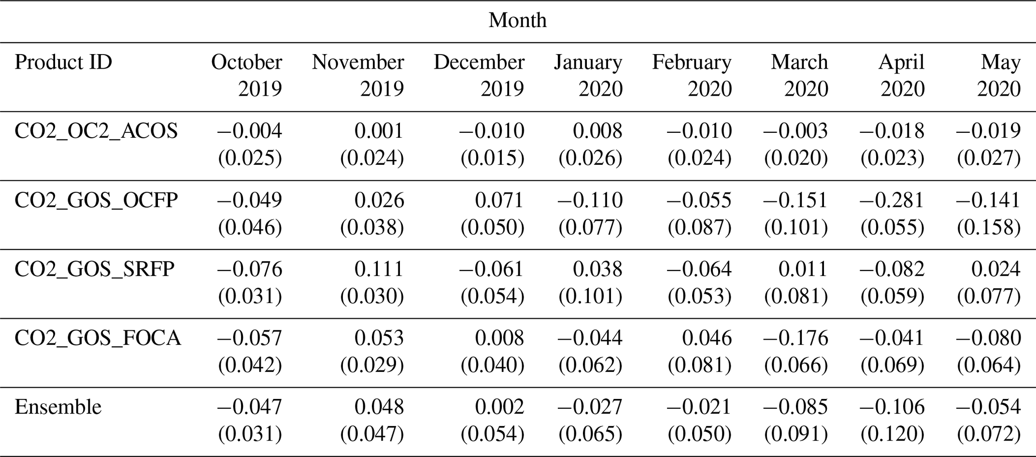
Table 4Numerical values of the ensemble-based CO $_{2}^{FF (DAM)}$ results as shown in Fig. 13. Listed are the median values and corresponding 1σ uncertainties (in brackets). The dimensionless values listed here represent the relative CO $_{2}^{FF (DAM)}$ change for January–May 2020 relative to October–December 2019 and previous years (OND anomalies; see main text).

Download Print Version | Download XLSX

5 Summary and conclusions

We have analysed a small ensemble of satellite XCO₂ data products to investigate whether a regional-scale reduction of atmospheric CO₂ during the COVID-19 pandemic can be detected for East China. Specifically, we analysed four XCO₂ data products from the satellites OCO-2 and GOSAT. For this purpose, we used a simple data-driven approach, which involves the computation of XCO₂ anomalies, ΔXCO₂, using a method called DAM (daily anomalies via (latitude band) medians). This method, which is essentially identical with the method developed at the Finnish Meteorological Institute (FMI, Hakkarainen et al., 2019), helps to isolate local or regional XCO₂ enhancements originating from anthropogenic CO₂ emissions from large-scale daily XCO₂ background variations (note however that the FMI method is not supposed to extract exclusively anthropogenic emission contributions to XCO₂; see Hakkarainen et al., 2019). In addition to the DAM method we also used a second method for the computation of ΔXCO₂, which is referred to as TmS (target minus surrounding). Using model and satellite data we found that the results obtained with the DAM method provide better results compared to the TmS method. Therefore, we focussed on DAM-based results but also report selected results obtained with the TmS method (reported separately in Appendix A). We analysed satellite data between January 2015 and May 2020 and compared year 2020 monthly XCO₂ anomalies with the corresponding monthly XCO₂ anomalies from previous periods.

In order to link the satellite-derived XCO₂ anomalies to East China fossil fuel (FF) CO₂ emissions, we used output from NOAA's CO₂ assimilation system CarbonTracker (CT2019) covering the years 2015 to 2018. We focus on October-to-May periods to minimize the impact of the terrestrial biosphere. Using CT2019, we show that ΔXCO₂ can be converted to FF emission estimates, denoted CO $_{2}^{FF}$ , via a linear transformation. The two coefficients slope and offset of this linear transformation have been obtained empirically via a linear fit; i.e. we established a linear empirical equation to relate the two quantities ΔXCO₂ and CO $_{2}^{FF}$ . We show using CT2019 that the retrieved emissions during October-to-May periods agree within 10 % with the CT2019 East China FF emissions.

For the analysis of the satellite data we focus on the October-2019-to-May-2020 period, which covers months during the COVID-19 pandemic but also pre-COVID-19 months. We compare results obtained during this period with earlier October-to-May periods to find out to what extent year 2020 differs from previous years. Our analysis is limited to October-to-May periods because our simple data-driven analysis method cannot deal with the large and highly variable terrestrial biosphere CO₂ fluxes outside of this period. On the other hand this period is challenging for satellite retrievals because of the low sun angles especially during the winter months and cloudiness.

We applied our method to each of the four satellite XCO₂ data products to obtain monthly emission estimates, CO $_{2}^{FF}$ , for East China. We focus on changes relative to pre-COVID-19 periods. Our results show considerable month-to-month variability (especially for the GOSAT products) and significant differences across the ensemble of satellite data products analysed. The ensemble mean suggests emission reductions by approximately 10 % ± 10 % in March and April 2020. This estimate is dominated by the GOSAT ensemble members. Analysis of the OCO-2 product yields smaller values, indicating a reduction of only about 1 %–2 % with an uncertainty of approximately ±2 %.

The large uncertainty, which is on the order of the derived reduction (i.e. 100 %, 1σ), and the large spread of the results obtained for the individual ensemble members indicate that it is challenging to reliably detect and to accurately quantify the emission reduction using the current generation of space-based methods and the simple DAM-based analysis strategy adopted here.

These findings, which are consistent with other recent studies (e.g. Chevallier et al., 2020; Zeng et al., 2020), are not unexpected. Regional XCO₂ enhancements due to fossil fuel emissions are typically only 1 to 2 ppm and even a 10 % emission reduction would therefore only correspond to a reduction of the fossil-fuel-related regional XCO₂ enhancement by 0.1 to 0.2 ppm. XCO₂ variations as small as 0.2 ppm are below the estimated uncertainty of the single footprint satellite XCO₂ retrievals. The uncertainty of single observations, which is typically around 0.7 ppm (e.g. Buchwitz et al., 2017a; Reuter et al., 2020), has been obtained by comparisons with ground-based Total Carbon Column Observing Network (TCCON) XCO₂ retrievals, which have an uncertainty of 0.4 ppm (1σ, Wunch et al., 2010). In this study we focus on monthly averaged data because our analysis method cannot properly deal with day-to-day variability and because of the sparseness of the satellite data. Averaging results in the reduction of the random error, but investigations have shown that random errors do not simply scale with the inverse of the square root of number of observations added due to (unknown) systematic errors and error correlations (Kulawik et al., 2016). Of course also other sources of uncertainty are relevant in this context, in particular time-dependent atmospheric transport and varying biogenic CO₂ contributions (e.g. Houweling et al., 2015, and references given therein).

We conclude that inferring COVID-19-related information on regional-scale CO₂ emissions using current (quite sparse) satellite XCO₂ retrievals requires, if at all possible, a more sophisticated analysis method including the use of detailed a priori information and atmospheric transport modelling.

The extent to which COVID-19-related emission reductions can be resolved on smaller scales – such as power plants or cities (e.g. Nassar et al., 2017; Reuter et al., 2019; Zheng et al., 2020a; Wu et al., 2020) has not been investigated in this study. For this purpose, XCO₂ retrievals from NASA's OCO-3 mission are promising, especially because of its Snapshot Area Map (SAM) mode, which permits the mapping of XCO₂ over ∼ 80 km by 80 km areas around localized anthropogenic CO₂ emission sources (see https://ocov3.jpl.nasa.gov/, last access: 28 August 2020). Even more complete coverage is planned for the Copernicus CO2M mission in the future (e.g. Janssens-Maenhout et al., 2020).

Appendix A

As explained in the main text, a second method has been applied to the CT2019 and the satellite data. This method is called “target minus surrounding” (TmS) and differs from the DAM method in the approach to determine the XCO₂ background. Whereas the DAM method computes the (daily) background as the median of the XCO₂ values in latitude bands, the TmS background is computed from the XCO₂ values in an area surrounding the target region (the coordinates are listed in Table 3).

The TmS results are discussed in the main text. Here we only show three figures. Figure A1 is the same as Fig. 2 but using the TmS method instead of the DAM method. Figure A2 is the TmS version of Fig. 7, and Fig. A3 is the TmS version of Fig. 13.

https://amt.copernicus.org/articles/14/2141/2021/amt-14-2141-2021-f14

Figure A1The same as Fig. 2 but using the target minus surrounding (TmS) method.

Download

https://amt.copernicus.org/articles/14/2141/2021/amt-14-2141-2021-f15

Figure A2The same as Fig. 7 but using the TmS method.

Download

https://amt.copernicus.org/articles/14/2141/2021/amt-14-2141-2021-f16

Figure A3The same as Fig. 13 but using the TmS method.

Download

Data availability

The key results of this study are listed in this paper in numerical form (Table 4). Access information for the satellite data used as input for this study is provided in Table 1. The CT2019 data are available from NOAA (see access information given in Table 2).

Author contributions

MB designed the study, performed the analysis and led the writing of this paper in close cooperation with MR, SN, BFA, HeB, JPB, OS, KB and MH. Input data and corresponding advice has been provided by MR, SN, ADN, HaB, LW, JL, IA, CWO'D, DC and CR. All authors contributed to significantly improve the manuscript.

Competing interests

The authors declare that they have no conflict of interest.

Acknowledgements

This study has been funded in parts by the European Space Agency (ESA) via projects ICOVAC (Impacts of COVID-19 lockdown measures on Air quality and Climate) and GHG-CCI+ (http://cci.esa.int/ghg, last access: 13 August 2020) and the University and the State of Bremen. We acknowledge financial support for the generation of several data sets used as input for this study from the following: (i) European Commission via Copernicus Climate Change Service (C3S, https://climate.copernicus.eu/, last access: 22 July 2020) project C3S_312b_Lot2, (ii) the Japanese space agency JAXA (contract 19RT000692) and (iii) EUMETSAT (contract EUM/CO/19/4600002372/RL). Hartmut Boesch, Univ. Leicester, was funded as part of NERC's support of the National Centre for Earth Observation (NE/R016518/1).

We also acknowledge access to OCO-2 XCO₂ data product OCO2_L2_Lite_FP 10r obtained from NASA's Earthdata GES DISC website (https://disc.gsfc.nasa.gov/datasets?keywords=OCO-2%20v10r&page=1, last access: 15 August 2020).

We thank JAXA and the National Institute for Environmental Studies (NIES), Japan, for access to GOSAT Level 1 (L1) data and ESA for making the GOSAT L1 products available via the ESA Third Party Mission (TPM) archive.

We acknowledge CarbonTracker CT2019 results provided by NOAA ESRL, Boulder, Colorado, USA, from the website at http://carbontracker.noaa.gov (last access: 22 July 2020). We also acknowledge feedback from Andy Jacobson on an early draft of the manuscript.

Some of the work reported here was conducted by the Jet Propulsion Laboratory, California Institute of Technology, under contract to NASA. Government sponsorship is acknowledged.

Financial support

This research has been supported by the European Space Agency via the projects ICOVAC (contract no. 4000127610/19/I-NS) and GHG-CCI+ (contract no. 4000126450/19/I-NB).

The article processing charges for this open-access publication were covered by the University of Bremen.

Review statement

This paper was edited by Ralf Sussmann and reviewed by three anonymous referees.

References

Agustí-Panareda, A., Diamantakis, M., Massart, S., Chevallier, F., Muñoz-Sabater, J., Barré, J., Curcoll, R., Engelen, R., Langerock, B., Law, R. M., Loh, Z., Morguí, J. A., Parrington, M., Peuch, V.-H., Ramonet, M., Roehl, C., Vermeulen, A. T., Warneke, T., and Wunch, D.: Modelling CO₂ weather – why horizontal resolution matters, Atmos. Chem. Phys., 19, 7347–7376, https://doi.org/10.5194/acp-19-7347-2019, 2019.

Basu, S., Guerlet, S., Butz, A., Houweling, S., Hasekamp, O., Aben, I., Krummel, P., Steele, P., Langenfelds, R., Torn, M., Biraud, S., Stephens, B., Andrews, A., and Worthy, D.: Global CO₂ fluxes estimated from GOSAT retrievals of total column CO₂, Atmos. Chem. Phys., 13, 8695–8717, https://doi.org/10.5194/acp-13-8695-2013, 2013.

Bauwens, M., Compernolle, S., Stavrakou, T., Müller, J.‐F., van Gent, J., Eskes, H., Levelt, P. F., van der A, R., Veefkind, J. P., Vlietinck, J., Yu, H., and Zehner, C.: Impact of coronavirus outbreak on NO₂ pollution assessed using TROPOMI and OMI observations, Geophys. Res. Lett., 47, e2020GL087978, https://doi.org/10.1029/2020GL087978, 2020.

Boesch, H., Anand, J., and Di Noia, A.: Product User Guide and Specification (PUGS) – ANNEX A for products CO_2_GOS_OCFP, CH4_GOS_OCFP & CH4_GOS_OCPR (v7.2, 2009–2018), available at: http://wdc.dlr.de/C3S_312b_Lot2/Documentation/GHG/PUGS/C3S_D312b_Lot2.3.2.3-v1.0_PUGS-GHG_ANNEX-A_v3.1.pdf (last access: 17 August 2020), 2019.

Bovensmann, H., Burrows, J. P., Buchwitz, M., Frerick, J., Noël, S., Rozanov, V. V., Chance, K. V., and Goede, A. H. P.: SCIAMACHY – Mission objectives and measurement modes, J. Atmos. Sci., 56, 127–150, 1999.

Bovensmann, H., Buchwitz, M., Burrows, J. P., Reuter, M., Krings, T., Gerilowski, K., Schneising, O., Heymann, J., Tretner, A., and Erzinger, J.: A remote sensing technique for global monitoring of power plant CO₂ emissions from space and related applications, Atmos. Meas. Tech., 3, 781–811, https://doi.org/10.5194/amt-3-781-2010, 2010.

Broquet, G., Bréon, F.-M., Renault, E., Buchwitz, M., Reuter, M., Bovensmann, H., Chevallier, F., Wu, L., and Ciais, P.: The potential of satellite spectro-imagery for monitoring CO₂ emissions from large cities, Atmos. Meas. Tech., 11, 681–708, https://doi.org/10.5194/amt-11-681-2018, 2018.

Buchwitz, M., Reuter, M., Bovensmann, H., Pillai, D., Heymann, J., Schneising, O., Rozanov, V., Krings, T., Burrows, J. P., Boesch, H., Gerbig, C., Meijer, Y., and Löscher, A.: Carbon Monitoring Satellite (CarbonSat): assessment of atmospheric CO₂ and CH₄ retrieval errors by error parameterization, Atmos. Meas. Tech., 6, 3477–3500, https://doi.org/10.5194/amt-6-3477-2013, 2013.

Buchwitz, M., Reuter, M., Schneising, O., Boesch, H., Guerlet, S., Dils, B., Aben, I., Armante, R., Bergamaschi, P., Blumenstock, T., Bovensmann, H., Brunner, D., Buchmann, B., Burrows, J. P., Butz, A., Chédin, A., Chevallier, F., Crevoisier, C. D., Deutscher, N. M., Frankenberg, C., Hase, F., Hasekamp, O. P., Heymann, J., Kaminski, T., Laeng, A., Lichtenberg, G., De Mazière, M., Noël, S., Notholt, J., Orphal, J., Popp, C., Parker, R., Scholze, M., Sussmann, R., Stiller, G. P., Warneke, T., Zehner, C., Bril, A., Crisp, D., Griffith, D. W. T., Kuze, A., O'Dell, C., Oshchepkov, S., Sherlock, V., Suto, H., Wennberg, P., Wunch, D., Yokota, T., and Yoshida, Y.: The Greenhouse Gas Climate Change Initiative (GHG-CCI): comparison and quality assessment of near-surface-sensitive satellite-derived CO₂ and CH₄ global data sets, Remote Sens. Environ., 162, 344–362, https://doi.org/10.1016/j.rse.2013.04.024, 2015.

Buchwitz, M., Reuter, M., Schneising, O., Hewson, W., Detmers, R. G., Boesch, H., Hasekamp, O. P., Aben, I., Bovensmann, H., Burrows, J. P., Butz, A., Chevallier, F., Dils, B., Frankenberg, C., Heymann, J., Lichtenberg, G., De Maziere, M., Notholt, J., Parker, R., Warneke, T., Zehner, C., Griffith, D. W. T., Deutscher, N. M., Kuze, A., Suto, H., and Wunch, D.: Global satellite observations of column-averaged carbon dioxide and methane: The GHG-CCI XCO₂ and XCH₄ CRDP3 data set, Remote Sens. Environ., 203, 276–295, https://doi.org/10.1016/j.rse.2016.12.027, 2017a.

Burrows, J. P., Hölzle, E., Goede, A. P. H., Visser, H., and Fricke, W.: SCIAMACHY – Scanning Imaging Absorption Spectrometer for Atmospheric Chartography, Acta Astronaut., 35, 445–451, https://doi.org/10.1016/0094-5765(94)00278-t, 1995.

Butz, A., Guerlet, S., Hasekamp, O., Schepers, D., Galli, A., Aben, I., Frankenberg, C., Hartmann, J.-M., Tran, H., Kuze, A., Keppel-Aleks, G., Toon, G., Wunch, D., Wennberg, P., Deutscher, N., Griffith, D., Macatangay, R., Messerschmidt, J., Notholt, J., and Warneke, T.: Toward accurate CO₂ and CH₄ observations from GOSAT, Geophys. Res. Lett., 38, L14812, https://doi.org/10.1029/2011GL047888, 2011.

Chevallier, F.: On the statistical optimality of CO₂ atmospheric inversions assimilating CO₂ column retrievals, Atmos. Chem. Phys., 15, 11133–11145, https://doi.org/10.5194/acp-15-11133-2015, 2015.

Chevallier, F., Palmer, P. I., Feng, L., Boesch, H., O'Dell, C. W., and Bousquet, P.: Towards robust and consistent regional CO₂ flux estimates from in situ and space-borne measurements of atmospheric CO₂, Geophys. Res. Lett., 41, 1065–1070, https://doi.org/10.1002/2013GL058772, 2014.

Chevallier, F., Zheng, B., Broquet, G., Ciais, P., Liu, Z., Davis, S. J., Deng, Z., Wang, Y., Bréon, F.-M., and O'Dell, C. W.: Local anomalies in the column-averaged dry air mole fractions of carbon dioxide across the globe during the first months of the coronavirus recession, Geophys. Res. Lett., 47, e2020GL090244, https://doi.org/10.1029/2020GL090244, 2020.

Ciais, P., Dolman, A. J., Bombelli, A., Duren, R., Peregon, A., Rayner, P. J., Miller, C., Gobron, N., Kinderman, G., Marland, G., Gruber, N., Chevallier, F., Andres, R. J., Balsamo, G., Bopp, L., Bréon, F.-M., Broquet, G., Dargaville, R., Battin, T. J., Borges, A., Bovensmann, H., Buchwitz, M., Butler, J., Canadell, J. G., Cook, R. B., DeFries, R., Engelen, R., Gurney, K. R., Heinze, C., Heimann, M., Held, A., Henry, M., Law, B., Luyssaert, S., Miller, J., Moriyama, T., Moulin, C., Myneni, R. B., Nussli, C., Obersteiner, M., Ojima, D., Pan, Y., Paris, J.-D., Piao, S. L., Poulter, B., Plummer, S., Quegan, S., Raymond, P., Reichstein, M., Rivier, L., Sabine, C., Schimel, D., Tarasova, O., Valentini, R., Wang, R., van der Werf, G., Wickland, D., Williams, M., and Zehner, C.: Current systematic carbon-cycle observations and the need for implementing a policy-relevant carbon observing system, Biogeosciences, 11, 3547–3602, https://doi.org/10.5194/bg-11-3547-2014, 2014.

Ciais, P., Crisp, D., Denier van der Gon, H., Engelen, R., Janssens-Maenhout, G., Heimann, H., Rayner, P., and Scholze, M.: Towards a European Operational Observing System to Monitor Fossil CO₂ emissions, Final Report from the expert group, European Comission, 68 pp., available at: https://edgar.jrc.ec.europa.eu/news_docs/CO2_report_22-10-2015.pdf (last access: 26 August 2020), 2015.

Cogan, A. J., Boesch, H., Parker, R. J., Feng, L., Palmer, P. I., Blavier, J.-F. L., Deutscher, N. M., Macatangay, R., Notholt, J., Roehl, C., Warneke, T., and Wunsch, D.: Atmospheric carbon dioxide retrieved from the Greenhouse gases Observing SATellite (GOSAT): Comparison with ground-based TCCON observations and GEOS-Chem model calculations, J. Geophys. Res., 117, D21301, https://doi.org/10.1029/2012JD018087, 2012.

Crisp, D., Atlas, R. M., Bréon, F.-M., Brown, L. R., Burrows, J. P., Ciais, P., Connor, B. J., Doney, S. C., Fung, I. Y., Jacob, D. J., Miller, C. E., O'Brien, D., Pawson, S., Randerson, J. T., Rayner, P., Salawitch, R. S., Sander, S. P., Sen, B., Stephens, G. L., Tans, P. P., Toon, G. C., Wennberg, P. O., Wofsy, S. C., Yung, Y. L., Kuang, Z., Chudasama, B., Sprague, G., Weiss, P., Pollock, R., Kenyon, D., and Schroll, S.: The Orbiting Carbon Observatory (OCO) mission, Adv. Space Res., 34, 700–709, 2004.

Crisp, D., Meijer, Y., Munro, R., Bowman, K., Chatterjee, A., Baker, D., Chevallier, F., Nassar, R., Palmer, P. I., Agusti-Panareda, A., Al-Saadi, J., Ariel, Y., Basu, S., Bergamaschi, P., Boesch, H., Bousquet, P., Bovensmann, H., Bréon, F.-M., Brunner, D., Buchwitz, M., Buisson, F., Burrows, J. P., Butz, A., Ciais, P., Clerbaux, C., Counet, P., Crevoisier, C., Crowell, S., DeCola, P. L., Deniel, C., Dowell, M., Eckman, R., Edwards, D., Ehret, G., Eldering, A., Engelen, R., Fisher, B., Germain, S., Hakkarainen, J., Hilsenrath, E., Holmlund, K., Houweling, S., Hu, H., Jacob, D., Janssens-Maenhout, G., Jones, D., Jouglet, D., Kataoka, F., Kiel, M., Kulawik, S. S., Kuze, A., Lachance, R. L., Lang, R., Landgraf, J., Liu, J., Liu, Y., Maksyutov, S., Matsunaga, T., McKeever, J., Moore, B., Nakajima, M., Natraj, V., Nelson, R. R., Niwa, Y., Oda, T., O'Dell, C. W., Ott, L., Patra, P., Pawson, S., Payne, V., Pinty, B., Polavarapu, S. M., Retscher, R., Rosenberg, R., Schuh, A., Schwandner, F. M., Shiomi, K., Su, W., Tamminen, J., Taylor, T. E., Veefkind, P., Veihelmann, B., Wofsy, S., Worden, J., Wunch, D., Yang, D., Zhang, P., and Zehner, C.: A Constellation Architecture for Monitoring Carbon Dioxide and Methane from Space, CEOS Atmospheric Composition Virtual Constellation Greenhouse Gas Team, Committee on Earth Observation Satellites, Version 1.0, 173 pp., available at: https://ceos.org/document_management/Virtual_Constellations/ACC/Documents/CEOS_AC-VC_GHG_White_Paper_Version_1_20181009.pdf (last access: 26 August 2020), 2018.

Dils, B., Buchwitz, M., Reuter, M., Schneising, O., Boesch, H., Parker, R., Guerlet, S., Aben, I., Blumenstock, T., Burrows, J. P., Butz, A., Deutscher, N. M., Frankenberg, C., Hase, F., Hasekamp, O. P., Heymann, J., De Mazière, M., Notholt, J., Sussmann, R., Warneke, T., Griffith, D., Sherlock, V., and Wunch, D.: The Greenhouse Gas Climate Change Initiative (GHG-CCI): comparative validation of GHG-CCI SCIAMACHY/ENVISAT and TANSO-FTS/GOSAT CO₂ and CH₄ retrieval algorithm products with measurements from the TCCON, Atmos. Meas. Tech., 7, 1723–1744, https://doi.org/10.5194/amt-7-1723-2014, 2014.

Eldering, A., Wennberg, P. O., Crisp, D., Schimel, D. S., Gunson, M. R., Chatterjee, A., Liu, J., Schwandner, F. M., Sun, Y., O'Dell, C. W., Frankenberg, C., Taylor, T., Fisher, B., Osterman, G. B., Wunch, D., Hakkarainen, J., Tamminen, J., and Weir, B.: The Orbiting Carbon Observatory-2 early science investigations of regional carbon dioxide fluxes, Science, 358, eaam5745, https://doi.org/10.1126/science.aam5745, 2017.

ESA: European Space Agency, Copernicus CO₂ Monitoring Mission Requirements Document, version 2.0 of 27/09/19, ESA Earth and Mission Science Division document ref. EOP-SM/3088/YM-ym, available at: https://esamultimedia.esa.int/docs/EarthObservation/CO2M_MRD_v2.0_Issued20190927.pdf (last access: 15 July 2020), 2019.

ESA-NASA-JAXA: ESA, NASA and JAXA COVID-10 Dashboard, available at: https://www.esa.int/ESA_Multimedia/Images/2020/06/COVID-19_Earth_Observation_Dashboard2 (last access: 15-March-2021), 2020.

Friedlingstein, P., Jones, M. W., O'Sullivan, M., Andrew, R. M., Hauck, J., Peters, G. P., Peters, W., Pongratz, J., Sitch, S., Le Quéré, C., Bakker, D. C. E., Canadell, J. G., Ciais, P., Jackson, R. B., Anthoni, P., Barbero, L., Bastos, A., Bastrikov, V., Becker, M., Bopp, L., Buitenhuis, E., Chandra, N., Chevallier, F., Chini, L. P., Currie, K. I., Feely, R. A., Gehlen, M., Gilfillan, D., Gkritzalis, T., Goll, D. S., Gruber, N., Gutekunst, S., Harris, I., Haverd, V., Houghton, R. A., Hurtt, G., Ilyina, T., Jain, A. K., Joetzjer, E., Kaplan, J. O., Kato, E., Klein Goldewijk, K., Korsbakken, J. I., Landschützer, P., Lauvset, S. K., Lefèvre, N., Lenton, A., Lienert, S., Lombardozzi, D., Marland, G., McGuire, P. C., Melton, J. R., Metzl, N., Munro, D. R., Nabel, J. E. M. S., Nakaoka, S.-I., Neill, C., Omar, A. M., Ono, T., Peregon, A., Pierrot, D., Poulter, B., Rehder, G., Resplandy, L., Robertson, E., Rödenbeck, C., Séférian, R., Schwinger, J., Smith, N., Tans, P. P., Tian, H., Tilbrook, B., Tubiello, F. N., van der Werf, G. R., Wiltshire, A. J., and Zaehle, S.: Global Carbon Budget 2019, Earth Syst. Sci. Data, 11, 1783–1838, https://doi.org/10.5194/essd-11-1783-2019, 2019.

Gier, B. K., Buchwitz, M., Reuter, M., Cox, P. M., Friedlingstein, P., and Eyring, V.: Spatially resolved evaluation of Earth system models with satellite column-averaged CO₂, Biogeosciences, 17, 6115–6144, https://doi.org/10.5194/bg-17-6115-2020, 2020.

Hakkarainen, J., Ialongo, I., and Tamminen, J.: Direct space-based observations of anthropogenic CO₂ emission areas from OCO-2, Geophys. Res. Lett., 43, 11400–11406, https://doi.org/10.1002/2016GL070885, 2016.

Hakkarainen, J., Ialongo, I., Maksyutov, S., and Crisp, D.: Analysis of Four Years of Global XCO₂ Anomalies as Seen by Orbiting Carbon Observatory-2, Remote Sens., 11, 850, https://doi.org/10.3390/rs11070850, 2019.

Houweling, S., Baker, D., Basu, S., Boesch, H., Butz, A., Chevallier, F., Deng, F., Dlugokencky, E. J., Feng, L., Ganshin, A., Hasekamp, O., Jones, D., Maksyutov, S., Marshall, J., Oda, T., O'Dell, C. W., Oshchepkov, S., Palmer, P. I., Peylin, P., Poussi, Z., Reum, F., Takagi, H., Yoshida, Y., and Zhuralev, R.: An intercomparison of inverse models for estimating sources and sinks of CO₂ using GOSAT measurements, J. Geophys. Res.-Atmos., 120, 5253–5266, https://doi.org/10.1002/2014JD022962, 2015.

IPCC: Climate Change 2013: The Physical Science Basis, Working Group I Contribution to the Fifth Assessment Report of the Intergovernmental Report on Climate Change, Cambridge University Press, Cambridge, UK, available at: http://www.ipcc.ch/report/ar5/wg1/ (last access: 21 February 2019), 2013.

Jacobson, A. R., Schuldt, K. N., Miller, J. B., Oda, T., Tans, P., Andrews, A., Mund, J., Ott, L., Collatz, G. J., Aalto, T., Afshar, S., Aikin, K., Aoki, S., Apadula, F., Baier, B., Bergamaschi, P., Beyersdorf, A., Biraud, S. C., Bollenbacher, A., Bowling, D., Brailsford, G., Abshire, J. B., Chen, G., Chen, H., Chmura, L., Colomb, A., Conil, S., Cox, A., Cristofanelli, P., Cuevas, E., Curcoll, R., Sloop, C. D., Davis, K., Wekker, S. D., Delmotte, M., DiGangi, J. P., Dlugokencky, E., Ehleringer, J., Elkins, J. W., Emmenegger, L., Fischer, M. L., Forster, G., Frumau, A., Galkowski, M., Gatti, L. V., Gloor, E., Griffis, T., Hammer, S., Haszpra, L., Hatakka, J., Heliasz, M., Hensen, A., Hermanssen, O., Hintsa, E., Holst, J., Jaffe, D., Karion, A., Kawa, S. R., Keeling, R., Keronen, P., Kolari, P., Kominkova, K., Kort, E., Krummel, P., Kubistin, D., Labuschagne, C., Langenfelds, R., Laurent, O., Laurila, T., Lauvaux, T., Law, B., Lee, J., Lehner, I., Leuenberger, M., Levin, I., Levula, J., Lin, J., Lindauer, M., Loh, Z., Lopez, M., Lund Myhre, C., Machida, T., Mammarella, I., Manca, G., Manning, A., Manning, A., Marek, M. V., Marklund, P., Martin, M. Y., Matsueda, H., McKain, K., Meijer, H., Meinhardt, F., Miles, N., Miller, C. E., Mölder, M., Montzka, S., Moore, F., Morgui, J.-A., Morimoto, S., Munger, B., Necki, J., Newman, S., Nichol, S., Niwa, Y., O'Doherty, S., Ottosson-Löfvenius, M., Paplawsky, B., Peischl, J., Peltola, O., Pichon, J.-M., Piper, S., Plass-Dölmer, C., Ramonet, M., Reyes-Sanchez, E., Richardson, S., Riris, H., Ryerson, T., Saito, K., Sargent, M., Sasakawa, M., Sawa, Y., Say, D., Scheeren, B., Schmidt, M., Schmidt, A., Schumacher, M., Shepson, P., Shook, M., Stanley, K., Steinbacher, M., Stephens, B., Sweeney, C., Thoning, K., Torn, M., Turnbull, J., Tørseth, K., Bulk, P. V. D., Laan-Luijkx, I. T. V. D., Dinther, D. V., Vermeulen, A., Viner, B., Vitkova, G., Walker, S., Weyrauch, D., Wofsy, S., Worthy, D., Young, D., and Zimnoch, M.: CarbonTracker CT2019, NOAA Earth System Research Laboratory, Global Monitoring Division, https://doi.org/10.25925/39m3-6069, 2020.

Janssens-Maenhout, G., Pinty, B., Dowell, M., Zunker, H., Andersson, E., Balsamo, G., Bezy, J.-L., Brunhes, T., Boesch, H., Bojkov, B., Brunner, D., Buchwitz, M., Crisp, D., Ciais, P., Counet, P., Dee, D., Denier van der Gon, H., Dolman, H., Drinkwater, M., Dubovik, O., Engelen, R., Fehr, T., Fernandez, V., Heimann, M., Holmlund, K., Houweling, S., Husband, R., Juvyns, O., Kentarchos, A., Landgraf, J., Lang, R., Loescher, A., Marshall, J., Meijer, Y., Nakajima, M., Palmer, P. I., Peylin, P., Rayner, P., Scholze, M., Sierk, B., Tamminen, J., and Veefkind P.: Towards an operational anthropogenic CO₂ emissions monitoring and verification support capacity, B. Am. Meteorol. Soc., 101, E1439–E1451, https://doi.org/10.1175/BAMS-D-19-0017.1, 2020.

Kaminski, T., Scholze, M., Voßbeck, M., Knorr, W., Buchwitz, M., and Reuter, M.: Constraining a terrestrial biosphere model with remotely sensed atmospheric carbon dioxide, Remote Sens. Environ., 203, 109–124, 2017.

Kiel, M., O'Dell, C. W., Fisher, B., Eldering, A., Nassar, R., MacDonald, C. G., and Wennberg, P. O.: How bias correction goes wrong: measurement of X_CO2 affected by erroneous surface pressure estimates, Atmos. Meas. Tech., 12, 2241–2259, https://doi.org/10.5194/amt-12-2241-2019, 2019.

Kuhlmann, G., Broquet, G., Marshall, J., Clément, V., Löscher, A., Meijer, Y., and Brunner, D.: Detectability of CO₂ emission plumes of cities and power plants with the Copernicus Anthropogenic CO₂ Monitoring (CO2M) mission, Atmos. Meas. Tech., 12, 6695–6719, https://doi.org/10.5194/amt-12-6695-2019, 2019.

Kulawik, S., Wunch, D., O'Dell, C., Frankenberg, C., Reuter, M., Oda, T., Chevallier, F., Sherlock, V., Buchwitz, M., Osterman, G., Miller, C. E., Wennberg, P. O., Griffith, D., Morino, I., Dubey, M. K., Deutscher, N. M., Notholt, J., Hase, F., Warneke, T., Sussmann, R., Robinson, J., Strong, K., Schneider, M., De Mazière, M., Shiomi, K., Feist, D. G., Iraci, L. T., and Wolf, J.: Consistent evaluation of ACOS-GOSAT, BESD-SCIAMACHY, CarbonTracker, and MACC through comparisons to TCCON, Atmos. Meas. Tech., 9, 683–709, https://doi.org/10.5194/amt-9-683-2016, 2016.

Kuze, A., Suto, H., Shiomi, K., Kawakami, S., Tanaka, M., Ueda, Y., Deguchi, A., Yoshida, J., Yamamoto, Y., Kataoka, F., Taylor, T. E., and Buijs, H. L.: Update on GOSAT TANSO-FTS performance, operations, and data products after more than 6 years in space, Atmos. Meas. Tech., 9, 2445–2461, https://doi.org/10.5194/amt-9-2445-2016, 2016.

Labzovskii, L. D., Jeong, S.-J., and Parazoo, N. C.: Working towards confident spaceborne monitoring of carbon emissions from cities using Orbiting Carbon Observatory-2, Remote Sens. Environ., 233, 111359, https://doi.org/10.1016/j.rse.2019.111359, 2019.

Lauer, A., Eyring, V., Righi, M., Buchwitz, M., Defourny, P., Evaldsson, M., Friedlingstein, P., de Jeu, R., de Leeuw, G., Loew, A., Merchant, C. J., Müller, B., Popp, T., Reuter, M., Sandven, S., Senftleben, D., Stengel, M., Van Roozendael, M., Wenzel, S., and Willén, U.: Benchmarking CMIP5 models with a subset of ESA CCI Phase 2 data using the ESMValTool, Remote Sens. Environ., 203, 9–39, https://doi.org/10.1016/j.rse.2017.01.007, 2017.

Le Quéré, C., Andrew, R. M., Friedlingstein, P., Sitch, S., Pongratz, J., Manning, A. C., Korsbakken, J. I., Peters, G. P., Canadell, J. G., Jackson, R. B., Boden, T. A., Tans, P. P., Andrews, O. D., Arora, V. K., Bakker, D. C. E., Barbero, L., Becker, M., Betts, R. A., Bopp, L., Chevallier, F., Chini, L. P., Ciais, P., Cosca, C. E., Cross, J., Currie, K., Gasser, T., Harris, I., Hauck, J., Haverd, V., Houghton, R. A., Hunt, C. W., Hurtt, G., Ilyina, T., Jain, A. K., Kato, E., Kautz, M., Keeling, R. F., Klein Goldewijk, K., Körtzinger, A., Landschützer, P., Lefèvre, N., Lenton, A., Lienert, S., Lima, I., Lombardozzi, D., Metzl, N., Millero, F., Monteiro, P. M. S., Munro, D. R., Nabel, J. E. M. S., Nakaoka, S., Nojiri, Y., Padin, X. A., Peregon, A., Pfeil, B., Pierrot, D., Poulter, B., Rehder, G., Reimer, J., Rödenbeck, C., Schwinger, J., Séférian, R., Skjelvan, I., Stocker, B. D., Tian, H., Tilbrook, B., Tubiello, F. N., van der Laan-Luijkx, I. T., van der Werf, G. R., van Heuven, S., Viovy, N., Vuichard, N., Walker, A. P., Watson, A. J., Wiltshire, A. J., Zaehle, S., and Zhu, D.: Global Carbon Budget 2017, Earth Syst. Sci. Data, 10, 405–448, https://doi.org/10.5194/essd-10-405-2018, 2018.

Le Quéré, C., Jackson, R. B., Jones, M. W., Smith, A. J. P., Abernethy, S., Andrew, R. M., De-Gol, A. J., Willis, D. R., Shan, Y., Canadell, J. G., Friedlingstein, P., Creutzig, G., and Peters, G. P.: Temporary reduction in daily global CO₂ emissions during the COVID-19 forced confinement, Nat. Clim. Change, 10, 647–653, https://doi.org/10.1038/s41558-020-0797-x, 2020.

Lespinas, F., Wang, Y., Broquet, G., Breon, F.-M., Buchwitz, M., Reuter, M., Meijer, Y., Loescher, A., Janssens-Maenhout, G., Zheng, B., and Ciais, P.: The potential of a constellation of low earth orbit satellite imagers to monitor worldwide fossil fuel CO₂ emissions from large cities and point sources, Carbon Balance Manage., 15, 18, https://doi.org/10.1186/s13021-020-00153-4, 2020.

Liu, J., Bowman, K. W., Schimel, D. S., Parazoo, N. C., Jiang, Z., Lee, M., Bloom, A. A., Wunch, D., Frankenberg, C., Sun, Y., O'Dell, C. W., Gurney, K. R., Menemenlis, D., Gierach, M., Crisp, D., and Eldering, A.: Contrasting carbon cycle responses of the tropical continents to the 2015–2016 El Niño, Science, 358, eaam5690, https://doi.org/10.1126/science.aam5690, 2017.

Liu, Z., Ciais, P., Deng, Z., Lei, R., Davis, S. J., Feng, S., Zheng, B., Cui, D., Dou, X., He, P., Zhu, B., Lu, C., Ke, P., Sun, T., Wang, Y., Yue, X., Wang, Y., Lei, Y., Zhou, H., Cai, Z., Wu, Y., Guo, R., Han, T., Xue, J., Boucher, O., Boucher, E., Chevallier, F., Wei, Y., Zhong, H., Kang, C., Zhang, N., Chen, B., Xi, F., Marie, F., Zhang, Q., Guan, D., Gong, P., Kammen, D. M., He, K., and Schellnhuber, H. J.: Near-real-time-data captured record decline in global CO₂ emissions due to COVID-19, arXiv [preprint], arXiv:2004.13614, 28 April 2020.

Massart, S., Agustí-Panareda, A., Heymann, J., Buchwitz, M., Chevallier, F., Reuter, M., Hilker, M., Burrows, J. P., Deutscher, N. M., Feist, D. G., Hase, F., Sussmann, R., Desmet, F., Dubey, M. K., Griffith, D. W. T., Kivi, R., Petri, C., Schneider, M., and Velazco, V. A.: Ability of the 4-D-Var analysis of the GOSAT BESD XCO₂ retrievals to characterize atmospheric CO₂ at large and synoptic scales, Atmos. Chem. Phys., 16, 1653–1671, https://doi.org/10.5194/acp-16-1653-2016, 2016.

Matsunaga, T. and Maksyutov, S.: A Guidebook on the Use of Satellite Greenhouse Gases Observation Data to Evaluate and Improve Greenhouse Gas Emission Inventories, Satellite Observation Center, National Institute for Environmental Studies, Japan, available at: https://www.nies.go.jp/soc/doc/GHG_Satellite_Guidebook_1st_12d.pdf (last access: 26 August 2020), 2018.

Miller, S. M. and Michalak, A. M.: The impact of improved satellite retrievals on estimates of biospheric carbon balance, Atmos. Chem. Phys., 20, 323–331, https://doi.org/10.5194/acp-20-323-2020, 2020.

Miller, S. M., Michalak, A. M., Detmers, R. G., Hasekamp, O. P., Bruhwiler, L. M. P., and Schwietzke, S.: China's coal mine methane regulations have not curbed growing emissions, Nat. Commun., 10, 303, https://doi.org/10.1038/s41467-018-07891-7, 2019.

Nassar, R., Hill, T. G., McLinden, C. A., Wunch, D., Jones, D. B. A., and Crisp, D.: Quantifying CO₂ emissions from individual power plants from space, Geophys. Res. Lett., 44, 10045–10053, https://doi.org/10.1002/2017GL074702, 2017.

Noël, S., Reuter, M., Buchwitz, M., Borchardt, J., Hilker, M., Bovensmann, H., Burrows, J. P., Di Noia, A., Suto, H., Yoshida, Y., Buschmann, M., Deutscher, N. M., Feist, D. G., Griffith, D. W. T., Hase, F., Kivi, R., Morino, I., Notholt, J., Ohyama, H., Petri, C., Podolske, J. R., Pollard, D. F., Sha, M. K., Shiomi, K., Sussmann, R., Té, Y., Velazco, V. A., and Warneke, T.: XCO₂ retrieval for GOSAT and GOSAT-2 based on the FOCAL algorithm, Atmos. Meas. Tech. Discuss. [preprint], https://doi.org/10.5194/amt-2020-453, in review, 2020.

O'Dell, C. W., Connor, B., Bösch, H., O'Brien, D., Frankenberg, C., Castano, R., Christi, M., Eldering, D., Fisher, B., Gunson, M., McDuffie, J., Miller, C. E., Natraj, V., Oyafuso, F., Polonsky, I., Smyth, M., Taylor, T., Toon, G. C., Wennberg, P. O., and Wunch, D.: The ACOS CO₂ retrieval algorithm – Part 1: Description and validation against synthetic observations, Atmos. Meas. Tech., 5, 99–121, https://doi.org/10.5194/amt-5-99-2012, 2012.

O'Dell, C. W., Eldering, A., Wennberg, P. O., Crisp, D., Gunson, M. R., Fisher, B., Frankenberg, C., Kiel, M., Lindqvist, H., Mandrake, L., Merrelli, A., Natraj, V., Nelson, R. R., Osterman, G. B., Payne, V. H., Taylor, T. E., Wunch, D., Drouin, B. J., Oyafuso, F., Chang, A., McDuffie, J., Smyth, M., Baker, D. F., Basu, S., Chevallier, F., Crowell, S. M. R., Feng, L., Palmer, P. I., Dubey, M., García, O. E., Griffith, D. W. T., Hase, F., Iraci, L. T., Kivi, R., Morino, I., Notholt, J., Ohyama, H., Petri, C., Roehl, C. M., Sha, M. K., Strong, K., Sussmann, R., Te, Y., Uchino, O., and Velazco, V. A.: Improved retrievals of carbon dioxide from Orbiting Carbon Observatory-2 with the version 8 ACOS algorithm, Atmos. Meas. Tech., 11, 6539–6576, https://doi.org/10.5194/amt-11-6539-2018, 2018.

Osterman, G., O'Dell, C., Eldering A., Fisher, B., Crisp, D., Cheng, C., Frankenberg, C., Lambert, A., Gunson, M., Mandrake, L., and Wunch, D.: Orbiting Carbon Observatory-2 and 3 (OCO-2 and OCO-3) Data Product User's Guide, Operational Level 2 Data Versions 10 and Lite File Version 10 and VEarly, Technical Report National Aeronautics and Space Administration, Jet Propulsion Laboratory, California Institute of Technology, Pasadena, USA, available at: https://docserver.gesdisc.eosdis.nasa.gov/public/project/OCO/OCO2_OCO3_B10_DUG.pdf, last access: 17 August 2020.

Palmer, P. I., Feng, L., Baker, D., Chevallier, F., Bösch, H., and Somkuti, P.; Net carbon emissions from African biosphere dominate pan-tropical atmospheric CO₂ signal, Nat. Commun., 10, 3344, https://doi.org/10.1038/s41467-019-11097-w, 2019.

Peters, W., Jacobson, A. R., Sweeney, C., Andrews, A. E., Conway, T. J., Masarie, K., Miller, J. B., Bruhwiler, L. M. P., Pétron, G., Hirsch, A. I., Worthy, D. E. J., van der Werf, G. R., Randerson, J. T., Wennberg, P. O., Krol, M. C., and Tans, P. P.: An atmospheric perspective on North American carbon dioxide exchange: CarbonTracker, P. Natl. Acad. Sci. USA, 104, 18925–18930, https://doi.org/10.1073/pnas.0708986104, 2007.

Pillai, D., Buchwitz, M., Gerbig, C., Koch, T., Reuter, M., Bovensmann, H., Marshall, J., and Burrows, J. P.: Tracking city CO₂ emissions from space using a high-resolution inverse modelling approach: a case study for Berlin, Germany, Atmos. Chem. Phys., 16, 9591–9610, https://doi.org/10.5194/acp-16-9591-2016, 2016.

Pinty, B., Janssens-Maenhout, G., Dowell, M., Zunker, H., Brunhes, T., Ciais, P., Dee, D., Denier van der Gon, H., Dolman, H., Drinkwater, M., Engelen, R., Heimann, M., Holmlund, K., Husband, R., Kentarchos, A., Meijer, Y., Palmer, P., and Scholze, M.: An Operational Anthropogenic CO₂ Emissions Monitoring and Verification Support capacity – Baseline Requirements, Model Components and Functional Architecture, European Commission Joint Research Centre, https://doi.org/10.2760/08644, 2017.

Pinty, B., Ciais, P., Dee, D., Dolman, H., Dowell, M., Engelen, R., Holmlund, K., Janssens-Maenhout, G., Meijer, Y., Palmer, P., Scholze, M., Denier van der Gon, H., Heimann, M., Juvyns, O., Kentarchos, A., and Zunker, H.: An Operational Anthropogenic CO₂ Emissions Monitoring and Verification Support Capacity – Needs and high level requirements for in situ measurements, European Commission Joint Research Centre, https://doi.org/10.2760/182790, 2019.

Reuter, M., Buchwitz, M., Schneising, O., Heymann, J., Bovensmann, H., and Burrows, J. P.: A method for improved SCIAMACHY CO₂ retrieval in the presence of optically thin clouds, Atmos. Meas. Tech., 3, 209–232, https://doi.org/10.5194/amt-3-209-2010, 2010.

Reuter, M., Bovensmann, H., Buchwitz, M., Burrows, J. P., Connor, B. J., Deutscher, N. M., Griffith, D. W. T., Heymann, J., Keppel-Aleks, G., Messerschmidt, J., Notholt, J., Petri, C., Robinson, J., Schneising, O., Sherlock, V., Velazco, V., Warneke, W., Wennberg, P. O., and Wunch, D.: Retrieval of atmospheric CO₂ with enhanced accuracy and precision from SCIAMACHY: Validation with FTS measurements and comparison with model results, J. Geophys. Res., 116, D04301, https://doi.org/10.1029/2010JD015047, 2011.

Reuter, M., Buchwitz, M., Hilker, M., Heymann, J., Schneising, O., Pillai, D., Bovensmann, H., Burrows, J. P., Bösch, H., Parker, R., Butz, A., Hasekamp, O., O'Dell, C. W., Yoshida, Y., Gerbig, C., Nehrkorn, T., Deutscher, N. M., Warneke, T., Notholt, J., Hase, F., Kivi, R., Sussmann, R., Machida, T., Matsueda, H., and Sawa, Y.: Satellite-inferred European carbon sink larger than expected, Atmos. Chem. Phys., 14, 13739–13753, https://doi.org/10.5194/acp-14-13739-2014, 2014a.

Reuter, M., Buchwitz, M., Hilboll, A., Richter, A., Schneising, O., Hilker, M., Heymann, J., Bovensmann, H., and Burrows, J. P.: Decreasing emissions of NOx relative to CO₂ in East Asia inferred from satellite observations, Nat. Geosci., 7, 792–795, https://doi.org/10.1038/ngeo2257, 2014b.

Reuter, M., Buchwitz, M., Schneising, O., Noël, S., Rozanov, V., Bovensmann, H., and Burrows, J. P.: A Fast Atmospheric Trace Gas Retrieval for Hyperspectral Instruments Approximating Multiple Scattering – Part 1: Radiative Transfer and a Potential OCO-2 XCO₂ Retrieval Setup, Remote Sens., 9, 1159, https://doi.org/10.3390/rs9111159, 2017a.

Reuter, M., Buchwitz, M., Schneising, O., Noël, S., Bovensmann, H., and Burrows, J. P.: A Fast Atmospheric Trace Gas Retrieval for Hyperspectral Instruments Approximating Multiple Scattering – Part 2: Application to XCO₂ Retrievals from OCO-2, Remote Sens., 9, 1102, https://doi.org/10.3390/rs9111102, 2017b.

Reuter, M., Buchwitz, M., Hilker, M., Heymann, J., Bovensmann, H., Burrows, J. P., Houweling, S., Liu, Y., Nassar, R., Chevallier, F., Ciais, P., Marshall, J., and Reichstein, M.: How much CO₂ is taken up by the European terrestrial biosphere?, B. Am. Meteorol. Soc., 98, 665–671, https://doi.org/10.1175/BAMS-D-15-00310.1, 2017c.

Reuter, M., Buchwitz, M., Schneising, O., Krautwurst, S., O'Dell, C. W., Richter, A., Bovensmann, H., and Burrows, J. P.: Towards monitoring localized CO₂ emissions from space: co-located regional CO₂ and NO₂ enhancements observed by the OCO-2 and S5P satellites, Atmos. Chem. Phys., 19, 9371–9383, https://doi.org/10.5194/acp-19-9371-2019, 2019.

Reuter, M., Buchwitz, M., Schneising, O., Noël, S., Bovensmann, H., Burrows, J. P., Boesch, H., Di Noia, A., Anand, J., Parker, R. J., Somkuti, P., Wu, L., Hasekamp, O. P., Aben, I., Kuze, A., Suto, H., Shiomi, K., Yoshida, Y., Morino, I., Crisp, D., O'Dell, C. W., Notholt, J., Petri, C., Warneke, T., Velazco, V. A., Deutscher, N. M., Griffith, D. W. T., Kivi, R., Pollard, D. F., Hase, F., Sussmann, R., Té, Y. V., Strong, K., Roche, S., Sha, M. K., De Mazière, M., Feist, D. G., Iraci, L. T., Roehl, C. M., Retscher, C., and Schepers, D.: Ensemble-based satellite-derived carbon dioxide and methane column-averaged dry-air mole fraction data sets (2003–2018) for carbon and climate applications, Atmos. Meas. Tech., 13, 789–819, https://doi.org/10.5194/amt-13-789-2020, 2020.

Schneising, O., Buchwitz, M., Burrows, J. P., Bovensmann, H., Reuter, M., Notholt, J., Macatangay, R., and Warneke, T.: Three years of greenhouse gas column-averaged dry air mole fractions retrieved from satellite – Part 1: Carbon dioxide, Atmos. Chem. Phys., 8, 3827–3853, https://doi.org/10.5194/acp-8-3827-2008, 2008.

Schneising, O., Heymann, J., Buchwitz, M., Reuter, M., Bovensmann, H., and Burrows, J. P.: Anthropogenic carbon dioxide source areas observed from space: assessment of regional enhancements and trends, Atmos. Chem. Phys., 13, 2445–2454, https://doi.org/10.5194/acp-13-2445-2013, 2013.

Schneising, O., Reuter, M., Buchwitz, M., Heymann, J., Bovensmann, H., and Burrows, J. P.: Terrestrial carbon sink observed from space: variation of growth rates and seasonal cycle amplitudes in response to interannual surface temperature variability, Atmos. Chem. Phys., 14, 133–141, https://doi.org/10.5194/acp-14-133-2014, 2014.

Schwandner, F. M., Gunson, M. R., Miller, C. E., Carn, S. A., Eldering, A., Krings, T., Verhulst, K. R., Schimel, D. S., Nguyen, H. M., Crisp, D., O'Dell, C. W., Osterman, G. B., Iraci, L. T., and Podolske, J. R.: Spaceborne detection of localized carbon dioxide sources, Science, 358, eaam5782, https://doi.org/10.1126/science.aam5782, 2017.

Sussmann, R. and Rettinger, M.: Can We Measure a COVID-19-Related Slowdown in Atmospheric CO₂ Growth? Sensitivity of Total Carbon Column Observations, Remote Sens., 12, 2387, https://doi.org/10.3390/rs12152387, 2020.

Tohjima, Y., Patra, P. K., Niwa, Y., Mukai, H., Sasakawa, M., and Machida, T.: Detection of fossil-fuel CO₂ plummet in China due to COVID-19 by observation at Hateruma, Sci. Rep., 10, 18688, https://doi.org/10.1038/s41598-020-75763-6, 2020.

Velazco, V. A., Buchwitz, M., Bovensmann, H., Reuter, M., Schneising, O., Heymann, J., Krings, T., Gerilowski, K., and Burrows, J. P.: Towards space based verification of CO₂ emissions from strong localized sources: fossil fuel power plant emissions as seen by a CarbonSat constellation, Atmos. Meas. Tech., 4, 2809–2822, https://doi.org/10.5194/amt-4-2809-2011, 2011.

Wu, D., Lin, J., Oda, T., and Kort, E.: Space-based quantification of per capita CO₂ emissions from cities, Environ. Res. Lett., 15, 035004, https://doi.org/10.1088/1748-9326/ab68eb, 2020.

Wu, L., Aben, I., and Hasekamp, O. P.: Product User Guide and Specification (PUGS) – ANNEX B for products CO2_GOS_SRFP, CH4_GOS_SRFP (v2.3.8, 2009–2018), available at: http://wdc.dlr.de/C3S_312b_Lot2/Documentation/GHG/PUGS/C3S_D312b_Lot2.3.2.3-v1.0_PUGS-GHG_ANNEX-B_v3.1.pdf (last access: 17 August 2020), 2019.

Wunch, D., Toon, G. C., Wennberg, P. O., Wofsy, S. C., Stephens, B. B., Fischer, M. L., Uchino, O., Abshire, J. B., Bernath, P., Biraud, S. C., Blavier, J.-F. L., Boone, C., Bowman, K. P., Browell, E. V., Campos, T., Connor, B. J., Daube, B. C., Deutscher, N. M., Diao, M., Elkins, J. W., Gerbig, C., Gottlieb, E., Griffith, D. W. T., Hurst, D. F., Jiménez, R., Keppel-Aleks, G., Kort, E. A., Macatangay, R., Machida, T., Matsueda, H., Moore, F., Morino, I., Park, S., Robinson, J., Roehl, C. M., Sawa, Y., Sherlock, V., Sweeney, C., Tanaka, T., and Zondlo, M. A.: Calibration of the Total Carbon Column Observing Network using aircraft profile data, Atmos. Meas. Tech., 3, 1351–1362, https://doi.org/10.5194/amt-3-1351-2010, 2010.

Wunch, D., Wennberg, P. O., Osterman, G., Fisher, B., Naylor, B., Roehl, C. M., O'Dell, C., Mandrake, L., Viatte, C., Kiel, M., Griffith, D. W. T., Deutscher, N. M., Velazco, V. A., Notholt, J., Warneke, T., Petri, C., De Maziere, M., Sha, M. K., Sussmann, R., Rettinger, M., Pollard, D., Robinson, J., Morino, I., Uchino, O., Hase, F., Blumenstock, T., Feist, D. G., Arnold, S. G., Strong, K., Mendonca, J., Kivi, R., Heikkinen, P., Iraci, L., Podolske, J., Hillyard, P. W., Kawakami, S., Dubey, M. K., Parker, H. A., Sepulveda, E., García, O. E., Te, Y., Jeseck, P., Gunson, M. R., Crisp, D., and Eldering, A.: Comparisons of the Orbiting Carbon Observatory-2 (OCO-2) X_CO2 measurements with TCCON, Atmos. Meas. Tech., 10, 2209–2238, https://doi.org/10.5194/amt-10-2209-2017, 2017.

Ye, X., Lauvaux, T., Kort, E. A., Oda, T., Feng, S., Lin, J. C., Yang, E. G., and Wu, D.: Constraining fossil fuel CO₂ emissions from urban area using OCO-2 observations of total column CO₂, J. Geophys. Res.-Atmos., 125, e2019JD030528, https://doi.org/10.1029/2019JD030528, 2020.

Yin, Y., Ciais, P., Chevallier, F., Li, W., Bastos, A., Piao, S., Wang, T., and Liu, H.: Changes in the response of the Northern Hemisphere carbon uptake to temperature over the last three decades, Geophys. Res. Lett., 45, 4371–4380, https://doi.org/10.1029/2018GL077316, 2018.

Zhang, R., Zhang, Y., Lin, H., Feng, X., Fu, T.-M., and Wang, Y.: NO_x Emission Reduction and Recovery during COVID-19 in East China, Atmosphere, 11, 433, https://doi.org/10.3390/atmos11040433, 2020.

Zheng, B., Chevallier, F., Ciais, P., Broquet, G., Wang, Y., Lian, J., and Zhao, Y.: Observing carbon dioxide emissions over China's cities and industrial areas with the Orbiting Carbon Observatory-2, Atmos. Chem. Phys., 20, 8501–8510, https://doi.org/10.5194/acp-20-8501-2020, 2020a.

Zheng, B., Geng, G., Ciais, P., Davis, S. J., Martin, R. V., Meng, J., Wu, N., Chevallier, F., Broquet, G., Boersma, F., van der A, R., Lin, J., Guan, D., Lei, Y., He, K., and Zhang, Q.: Satellite-based estimates of decline and rebound in China's CO₂ emissions during COVID-19 pandemic, Sci. Adv., 6, eabd4998, https://doi.org/10.1126/sciadv.abd4998, 2020b.

Zeng, N., Han, P., Liu, D., Liu, Z., Oda, T., Martin, C., Liu, Z., Yao, B., Sun, W., Wang, P., Cai, Q., Dickerson, R., and Maksyutov, S.: Global to local impacts on atmospheric CO₂ caused by COVID-19 lockdown, arXiv [preprint], arXiv:2010.13025, 25 October 2020.

Articles

Short summary

The COVID-19 pandemic resulted in reduced anthropogenic carbon dioxide (CO₂) emissions during 2020 in large parts of the world. We have used a small ensemble of satellite retrievals of column-averaged CO₂ (XCO₂) to find out if a regional-scale reduction of atmospheric CO₂ can be detected from space. We focus on East China and show that it is challenging to reliably detect and to accurately quantify the emission reduction, which only results in regional XCO₂ reductions of about 0.1–0.2 ppm.

Can a regional-scale reduction of atmospheric CO2 during the COVID-19 pandemic be detected from space? A case study for East China using satellite XCO2 retrievals

2.1 Satellite XCO2 retrievals

2.2 Model CO2 data

3.1 Methods to compute XCO2 anomalies (ΔXCO2)

3.2 Computation of emission estimates (CO2FF)

4.1 Application of the DAM method to satellite XCO2 retrievals

4.2 Emission estimates

4.2.1 Emission estimates from NASA's OCO-2 (version 10r) XCO2

4.2.2 Emission estimates from GOSAT XCO2 data products

4.2.3 Ensemble mean and uncertainty

Can a regional-scale reduction of atmospheric CO₂ during the COVID-19 pandemic be detected from space? A case study for East China using satellite XCO₂ retrievals

2.1 Satellite XCO₂ retrievals

2.2 Model CO₂ data

3.1 Methods to compute XCO₂ anomalies (ΔXCO₂)

3.2 Computation of emission estimates (CO $_{2}^{FF}$ )

4.1 Application of the DAM method to satellite XCO₂ retrievals

4.2.1 Emission estimates from NASA's OCO-2 (version 10r) XCO₂

4.2.2 Emission estimates from GOSAT XCO₂ data products