the Creative Commons Attribution 4.0 License.
the Creative Commons Attribution 4.0 License.
 | 06 Jul 2018
Comparing OMI-based and EPA AQS in situ NO2 trends: towards understanding surface NOx emission changes
Ruixiong Zhang
Charles Smeltzer
Hang Qu
William Koshak
K. Folkert Boersma
With the improved spatial resolution of the Ozone Monitoring Instrument (OMI) over earlier instruments and more than 10 years of service, tropospheric NO2 retrievals from OMI have led to many influential studies on the relationships between socioeconomic activities and NOx emissions. Previous studies have shown that the OMI NO2 data show different relative trends compared to in situ measurements. However, the sources of the discrepancies need further investigations. This study focuses on how to appropriately compare relative trends derived from OMI and in situ measurements. We retrieve OMI tropospheric NO2 vertical column densities (VCDs) and obtain the NO2 seasonal trends over the United States, which are compared with coincident in situ surface NO2 measurements from the Air Quality System (AQS) network. The Mann–Kendall method with Sen's slope estimator is applied to derive the NO2 seasonal and annual trends for four regions at coincident sites during 2005–2014. The OMI-based NO2 seasonal relative decreasing trends are generally biased low compared to the in situ trends by up to 3.7 % yr−1, except for the underestimation in the US Midwest and Northeast during December, January, and February (DJF). We improve the OMI retrievals for trend analysis by removing the ocean trend, using the Moderate Resolution Imaging Spectroradiometer (MODIS) albedo data in air mass factor (AMF) calculation. We apply a lightning flash filter to exclude lightning-affected data to make proper comparisons. These data processing procedures result in close agreement (within 0.3 % yr−1) between in situ and OMI-based NO2 regional annual relative trends. The remaining discrepancies may result from inherent difference between trends of NO2 tropospheric VCDs and surface concentrations, different spatial sampling of the measurements, chemical nonlinearity, and tropospheric NO2 profile changes. We recommend that future studies apply these procedures (ocean trend removal and MODIS albedo update) to ensure the quality of satellite-based NO2 trend analysis and apply the lightning filter in studying surface NOx emission changes using satellite observations and in comparison with the trends derived from in situ NO2 measurements. With these data processing procedures, we derive OMI-based NO2 regional annual relative trends using all available data for the US West (−2.0 % ± 0.3 yr−1), Midwest (−1.8 % ± 0.4 yr−1), Northeast (−3.1 % ± 0.5 yr−1), and South (−0.9 % ± 0.3 yr−1). The OMI-based annual mean trend over the contiguous United States is −1.5 % ± 0.2 yr−1. It is a factor of 2 lower than that of the AQS in situ data (−3.9 % ± 0.4 yr−1); the difference is mainly due to the fact that the locations of AQS sites are concentrated in urban and suburban regions.
- Article
(3356 KB) -
Supplement
(276 KB) - BibTeX
- EndNote


Nitrogen dioxide (NO2) is an air pollutant. At high concentrations, it aggravates respiratory diseases and can lead to acid rain formation (e.g., Lamsal et al., 2015). It is also a key player in producing another pollutant, ozone (O3), through photochemical reactions in the presence of volatile organic compounds (VOCs) in sunlight. Tropospheric NO2 is emitted both anthropogenically and naturally (e.g., Gu et al., 2016). Anthropogenic fossil fuel combustions and biomass burning emit mostly nitrogen monoxide (NO) at high temperature, which is later oxidized by O3 into NO2. Major natural NO2 sources include lightning and soils.
Surface NO2 concentrations are regulated by the US Environmental Protection Agency (EPA) through the National Ambient Air Quality Standards (NAAQS). NO2 is measured routinely at the EPA Air Quality System (AQS) sites (Demerjian, 2000). Although the AQS network continually provides valuable hourly NO2 measurements, AQS sites are mostly located in urban and suburban regions, leaving large regions of rural areas unmonitored. Satellite data provide better spatial coverage than the in situ measurements.
Several satellites have been launched to monitor tropospheric NO2 vertical column densities (VCDs), such as the SCanning Imaging Absorption spectroMeter for Atmospheric CHartographY (SCIAMACHY), the Global Ozone Monitoring Experiment–2 (GOME-2), and the Ozone Monitoring Instrument (OMI). For trend analysis, the tropospheric NO2 products from OMI surpass the others for a relatively high spatial resolution and over 1 decade of continuous operation (Boersma et al., 2004, 2011). Thus, OMI NO2 retrievals are widely applied in NO2 and NOx emission trend studies (e.g., Lin et al., 2010, 2013; Lin and McElroy, 2011; Castellanos and Boersma, 2012; Russell et al., 2012; Gu et al., 2013; Lamsal et al., 2015; Lu et al., 2015; Tong et al., 2015; Cui et al., 2016; Duncan et al., 2016; de Foy et al., 2016a, b; Krotkov et al., 2016; Liu et al., 2017). Tong et al. (2015) reported that the reduction rates calculated from OMI NO2 VCDs and AQS surface NO2 data in eight cities were −35 and −38 % from 2005 to 2012, respectively. Lamsal et al. (2015) also found the divergence between the annual trends inferred from the two datasets, i.e., −4.8 % yr−1 vs. −3.7 % yr−1 during 2005–2008, and −1.2 % yr−1 vs. −2.1 % yr−1 during 2010–2013. There are several potential factors that contribute to the discrepancies between trends from satellite and ground-based measurements: interferences by the oxidation products of NOx from the chemiluminescent instruments (Lamsal et al., 2008, 2014, 2015), the differences of sampling time between OMI (∼ 13:30 local time) and AQS (hourly) measurements (Tong et al., 2015), a high sensitivity of NO2 VCDs to high-altitude NO2 in contrast to the high sensitivity of surface NO2 concentrations to surface NOx emissions (Duncan et al., 2013; Lamsal et al., 2015), spatial representativeness of satellite pixels (Lamsal et al., 2015), and high uncertainties of satellite retrievals in clean regions (Lamsal et al., 2015).
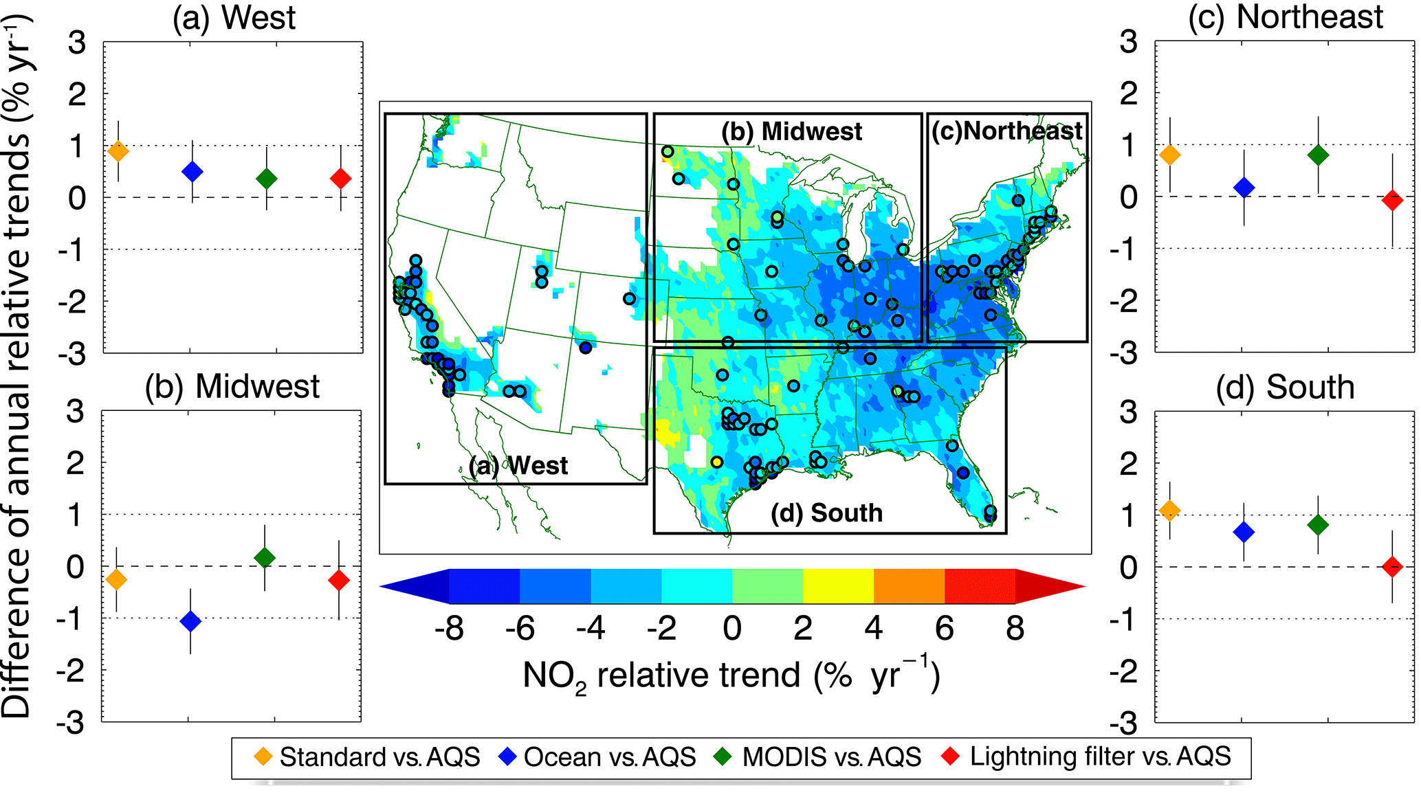
Figure 1The solid black borders in the center map define the four regions used in this study. The colored background shows the OMI-based NO2 annual relative trends of the “lightning filter” data. Grid cells with 2005–2014 mean NO2 VCD values < 1 × 10¹⁵ molecules cm−2 are excluded in this study and are shown in white. The black-bordered circles represent the locations of AQS sites. Panel (a) through (d) show the regional difference (OMI-based relative trends minus AQS relative trends) of annual relative trends between coincident OMI-based and AQS in situ data. The colored diamonds are for “standard” (orange), “ocean” (blue), “MODIS” (green), and “lightning filter” (red) OMI data. The different OMI VCD data are described in Sect. 2.4.
To understand how various factors and the retrieval procedure affect the differences between the OMI-derived trends and those derived from the surface AQS measurements, we utilize a regional 3-D chemistry transport model (CTM), a radiative transfer model (RTM), and the Mann–Kendall method (Mann, 1945; Kendall, 1948) to calculate OMI-based NO2 seasonal relative trends during December, January, and February (DJF); March, April, and May (MAM); June, July, and August (JJA); and September, October, and November (SON) (Sect. 2). We find that two procedures are essential to ensure the quality of trend analysis using OMI tropospheric NO2 VCDs, including the ocean trend removal and the Moderate Resolution Imaging Spectroradiometer (MODIS) albedo update in calculating the air mass factors (AMFs). The lightning filter (Sect. 3.1) is necessary for comparing OMI-based and in situ AQS NO2 trends. With these procedures implemented, the differences between OMI-based and AQS in situ annual relative trends are within 0.3 % yr−1 of coincident measurements for all the four regions. Finally, we estimate the OMI-based annual relative trends across the nation in Sect. 3.2. Conclusions are given in Sect. 4.
2.1 EPA AQS surface NO2 measurements
The in situ surface NO2 measurements from the US EPA AQS network are used in this research. Sites with a continuous measurement gap of more than 50 days are removed, and the observations of 140 remaining cites are used (Fig. 1). The AQS chemiluminescent analyzers are equipped with molybdenum converters to measure ambient NO2 concentrations. These analyzers are known to have high biases, since the converters are not NO2 specific and they measure some fractions of peroxyacetyl nitrate, nitric acid, and organic nitrates (Demerjian, 2000; Lamsal et al., 2008). In addition to chemiluminescent analyzers, several NO2-specific photolytic instruments have been deployed since 2013. By utilizing the data from both chemiluminescent and photolytic measurements at coincident sites during the overpassing time of OMI, we calculate the observed NO2 concentration ratio between both measurements in Fig. S1 in the Supplement. The ratio peaks at 2.3 in June and decreases to 1.3 in November, indicating that the chemiluminescent analyzers overestimate by 27–132 % as compared to photolytic instruments. This finding is in agreement with Lamsal et al. (2008). We correct the chemiluminescent NO2 data by the observed ratio, assuming that the interannual change is small and the high bias of the chemiluminescent measurements is identical at all sites. This correction may contribute to the differences between in situ and OMI-based absolute NO2 trends but does not significantly affect the relative trends (since the correction is canceled out in computing relative trends). In this study, we only examine the relative trends, and therefore the analysis results are not affected by the uncertainties in the in situ NO2 measurement corrections.
2.2 REAM model
We use the 3-D Regional chEmical trAnsport Model (REAM) in the simulation of NO2 profiles. REAM has widely been used in atmospheric NO2 studies, including vertical transport (Choi et al., 2005; Zhao et al., 2009; Zhang et al., 2016), emission inversions (Zhao and Wang, 2009; Yang et al., 2011; Gu et al., 2013, 2014, 2016), and regional and seasonal variations (Choi et al., 2008a, b). The model has a horizontal resolution of 36 km with 30 vertical layers in the troposphere, 5 vertical layers in the stratosphere, and a model top of 10 hpa. In this study, the domain of REAM is about 400 km larger on each side than the contiguous United States (CONUS). Meteorology inputs driving the transport process are simulated by the Weather Research and Forecasting model (WRF) assimilations constrained by National Centers for Environmental Prediction Climate Forecast System Reanalysis (NCEP CFSR; Saha et al., 2010) 6-hourly products. The KF-Eta scheme is used for sub-grid convective transport in WRF (Kain and Fritsch, 1993). We run the WRF model with the same resolution as in REAM but with a domain 10 grids larger on each side than that of REAM. REAM updates most of the meteorology inputs every 30 min, while those related to convective transport and lightning parameterization are updated every 5 min. The chemistry mechanism expands upon that of the global CTM GEOS-Chem (V9-02) with aromatic chemistry (Bey et al., 2001; Liu et al., 2010, 2012a, b; Zhang et al., 2017). For consistency, the GEOS-Chem (V9-02) simulation with 2∘ × 2.5∘ resolution is used to generate initial and boundary conditions for chemical tracers.
Anthropogenic emissions of NOx and other chemical species are from the US National Emission Inventory 2008 prepared using the Sparse Matrix Operator Kernel Emission (SMOKE) model. Biogenic emissions are simulated online using the Model of Emissions of Gases and Aerosols from Nature (MEGAN) algorithm (v2.1; Guenther et al., 2012). We parameterize lightning-emitted NOx as a function of convective mass flux and convective available potential energy (CAPE) (Choi et al., 2005). NOx production per flash is set to 250 moles NO per flash, and the emissions are distributed vertically following the C-shaped profiles by Pickering et al. (1998). For recent model evaluations of REAM with observations, we refer readers to Zhang et al. (2016), Zhang and Wang (2016), Cheng et al. (2017), and Zhang et al. (2017).
2.3 OMI-based NO2 VCDs
We retrieve the tropospheric NO2 VCDs using the tropospheric slant column densities (SCDs, without destriping) from the Royal Dutch Meteorological Institute (KNMI) Dutch OMI NO2 product (DOMINO v2; Boersma et al., 2011). OMI on board the Aura satellite was launched in July 2004 and is still active. OMI overpasses the Equator at about 13:30 local time (LT) and obtains global coverage with a 2600 km viewing swath spanning 60 rows. It has a ground level spatial resolution up to 13 km × 24 km (at nadir). The spatial extent of the OMI pixels will not affect our analysis as we focus on regional trend analysis. SCDs are retrieved by matching a modeled spectrum to an observed top-of-atmosphere reflectance with the differential optical absorption spectroscopy (DOAS) technique within a fitting window of 405–465 nm. The stratospheric portion of SCDs is estimated and subsequently removed with the global CTM TM4 with stratospheric ozone assimilation (Dirksen et al., 2011). Deriving tropospheric VCDs from the remaining tropospheric SCDs requires the calculation of AMFs. Since NO2 is an optically thin gas, tropospheric AMF for NO2 can be calculated from AMF for each vertical layer (AMFl) weighted by NO2 partial VCDs at the corresponding layer (xl) (Boersma et al., 2004), as shown in Eq. (1).
As the vertical distribution of NO2 is usually unknown, we typically substitute xl by an a priori profile (xl, apriori) from a CTM. AMFl is the sensitivity of NO2 SCD to VCD at a given altitude (Eskes and Boersma, 2003) and is computed using the Double-Adding KNMI (DAK) RTM (Boersma et al., 2011). As a result, the retrieved tropospheric NO2 VCD computation depends on the a priori NO2 vertical profile, the surface reflectance, the surface pressure, the temperature profile, and the viewing geometry (Boersma et al., 2011). Previous studies have addressed the sources of uncertainties in NO2 retrievals, including surface reflectance resolutions (Russell et al., 2011; Lin et al., 2014), lightning NOx (Choi et al., 2005; Martin et al., 2007; Bucsela et al., 2010), a priori CTM uncertainties (Russell et al., 2011; Heckel et al., 2011; Lin et al., 2012; Laughner et al., 2016), surface pressure and reflectance anisotropy in rugged terrain (Zhou et al., 2009), cloud and aerosol radiance (Lin et al., 2014, 2015), and boundary layer dynamics (Zhang et al., 2016). In this study, we find that the first two factors are essential in NO2 VCD trend analysis, and we will discuss these in the following sections.
AMFs are derived using the pre-computed altitude-dependent AMF lookup table, which is generated by the DAK RTM. We use the NO2 profiles from REAM, temperature and pressure from CSFR, and viewing geometry and cloud information from the DOMINO v2 product. We use the REAM results of 2010 to avoid the uncertainty introduced by yearly variation of NO2 profiles. The yearly variations of meteorology and anthropogenic emission changes have little impact in polluted areas on trend analysis results using OMI data (Lamsal et al., 2015). We use the surface reflectance from the DOMINO v2 product as a default (Kleipool et al., 2008) and update it using a surface reflectance product with a higher temporal resolution (Sect. 2.3.2). The derived tropospheric NO2 VCD relative trends with default surface reflectance are referred to as “standard”.
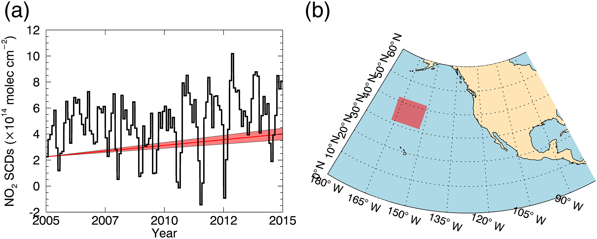
Figure 2The black line in panel (a) shows the monthly averaged OMI tropospheric NO2 VCD values in the North Pacific region (red box in panel b) from 2005 to 2014. The red line in panel (a) represents the ocean trend used in this research, with the 95th-percentile confidence intervals shaded in red.
2.3.1 Ocean trend removal
For trend and other analyses of OMI tropospheric VCDs, the data of anomalous pixels must be removed. The row anomaly initially occurred in June 2007 and subsequently in later years affected rows 26–40 (Schenkeveld et al., 2017). Additional anomalies can be found in some years in rows 41–55. For trend analysis from 2005 to 2014, we exclude rows 26–55, consistent with our understanding of the row anomaly (Schenkeveld et al., 2017). In addition, the data of coarse spatial resolution from rows 1 to 5 and rows 56 to 60 are also excluded, as suggested by Lamsal et al. (2015). The selection of rows 6–25 used in this research is stricter than the data flags in the DOMINO v2 product. Furthermore, we exclude OMI data with cloud fraction > 0.3 to minimize retrieval uncertainties due to clouds and aerosols (Boersma et al., 2011; Lin et al., 2014).
Figure 2a shows that there is an apparent increasing trend of the averaged tropospheric SCDs in the remote ocean region (Fig. 2b) with minimal marine traffic. This trend may reflect the inaccurately simulated stratospheric SCDs or the increase in the magnitude of the stripes (step-wise SCD variability from one row to another) in time, which originates from the use of a constant (2005-averaged) solar irradiance reference spectrum in the DOAS spectral fits throughout the mission and the weak increase of noise in the OMI radiance measurements (K. Folkert Boersma, personal communication, 2017; Zara et al., 2018). Figure 2a shows that there is a positive annual trend of 1.75 ± 0.45 × 10¹³ molecules cm−2 yr−1. The ocean trend is insensitive to the region selection in the remote North Pacific (varies within 10 %). We only analyze OMI tropospheric column trends over the CONUS for grid cells with 2005–2014-averaged VCDs > 1 × 10¹⁵ molecules cm−2, which tends to minimize the effect of the background noise. However, removing this background ocean (absolute) trend has a non-negligible effect in reducing the OMI relative trend (Fig. 1). We treat this trend as a systematic bias. We calculate the contribution from the ocean (absolute) annual trend to SCDs for each year and subtract it from OMI tropospheric NO2 SCDs uniformly in the following analysis. Since the origin of this trend is not yet clear, the ocean trend removal method may need updates in future studies. We refer to such derived (relative) trend data as “ocean”. An alternative method is to subtract monthly SCD trends of the remote ocean region (Fig. S2 in the Supplement) from the OMI tropospheric SCD data. Although the end results (Fig. S3 in the Supplement) are essentially the same as the annual trend removal method, noises are added to the SCD data, making it more difficult to understand the effects of the MODIS albedo update and the lightning filter (next sections). We therefore choose to use the (absolute) annual trend removal method here.
2.3.2 MODIS albedo update
The albedo data used to calculate the AMFl in standard and ocean versions of trend analysis are from the DOMINO v2 products, which are the climatology of averaged OMI measurements during 2005–2009 with a spatial resolution of 0.5∘ × 0.5∘ (Kleipool et al., 2008) and are valid for 440 nm. We recalculate the AMFl using the MODIS 16-day MCD43B3 albedo product with 1 km spatial resolution, which combines data from MODIS on board both Aqua and Terra satellites (Schaaf et al., 2002; Tang et al., 2007). Aqua and Terra have an equatorial overpassing time of 13:30 and 10:30 LT, respectively. The band 3 (459–479 nm) is used to match the NO2 fitting window (405–465 nm). The albedo is spatially integrated to the geometry of OMI pixels and is temporally interpolated to match OMI overpassing dates. In order to maintain the consistency of the DOMINO retrieval algorithm (Boersma et al., 2011), we only use the MODIS data to improve the temporal variations of albedo data used in the retrieval. We scale the MODIS albedo data such that the mean albedo during 2005–2009 is the same as the OMI climatology at 0.5∘ × 0.5∘. We recalculate OMI tropospheric VCDs using the MODIS albedo data as described. We recalculate the relative OMI trend and remove the ocean (absolute) trend (Sect. 2.3.1). We refer to this version of OMI relative trend data as “MODIS”.
2.3.3 Lightning event filter
Over North America, lightning is a major source of NOx in the free troposphere, and its simulations in CTMs are uncertain (e.g., Zhao et al., 2009; Luo et al., 2017). The large temporospatial variations of lightning NOx make it difficult to compute satellite-based NO2 trends by changing the vertical distributions of NO2 affecting the AMF calculation (e.g., Choi et al., 2008b; Lamsal et al., 2010) and the SCD values. Furthermore, accompanying lightning occurrences, the presence of cloud significantly affects the lifetime of NOx and the partitioning of NO2 to NO in daytime, and convective transport exports NOx from the surface and boundary layer to the free troposphere, changing surface and column NO2 concentrations. Given the difficulty to simulate lightning NOx accurately across different years and meteorological effects (vertical mixing) of lightning, we use a lightning filter to remove potential effects of lightning NOx on the basis of the flash rate observations of cloud-to-ground (CG) lightning flash data detected by the National Lightning Detection Network™ (NLDN) (Cummins and Murphy, 2009; Rudlosky and Fuelberg, 2010). NLDN only reports the ground point of a CG lightning flash, while the CG lightning flash can extend horizontally to tens of kilometers. A CG lightning flash can affect the NO2 retrievals not only in the model grid cell where the CG lightning is located but also the nearby model grid cells. The atmospheric lifetime of NOx in the free troposphere can be up to 1 week. Therefore, we exclude the OMI NO2 data within a radius of 90 km of the NLDN-reported CG lightning location (about two model grid cells around the grid cell where the CG lightning is located) for a period of 72 h after the lightning occurrence. Since lightning usually occurs along the track of a thunderstorm, the 90 km radius is more of a constraint on lightning NOx effects across the track. The extended period of 72 h is to ensure that we exclude data affected by lightning NOx. Figure 4 shows the distribution of the number of days of 2005–2014 with lightning detection. The Southwest monsoon and the South regions have more lightning days than the other areas. While there are fewer lightning flashes in the Northeast than the South (Fig. 3), large amounts of lightning NOx can be produced by high flash ratios of severe thunderstorms, and they can be transported northward from the South to the Northeast (Choi et al., 2005). We therefore further filter OMI NO2 data in the Northeast on the basis of CG lightning flash rates in the South. If the average CG flash rate in the South exceeds the 95th-percentile value of the NLDN observations, which is 0.035 flash km−2 day−1 (Fig. S4 in the Supplement), we exclude in the analysis the Northeast OMI data in the following 72 h. Excluding the OMI data based on CG lightning data implicitly removes the data affected by cloud-to-cloud lightning collocated with CG lightning. The lightning filter removes about 2, 27, 20, and 19 % of OMI data, which are coincident with AQS data for the West, the Midwest, the Northeast, and the South, respectively. We refer to this version of OMI relative trend data as “lightning filter”.

Figure 3Number of days with NLDN-detected cloud-to-ground (CG) lightning per model grid cell per year during 2005–2014. The lightning occurrences are calculated using the REAM grid resolution.
We group the analysis results into different regions: (a) West, (b) Midwest, (c) Northeast, and (d) South (Fig. 1), following the regional divisions by the United States Census Bureau. To make a fair comparison between the in situ and OMI-based trends, we only use spatially and temporally coincident in situ and OMI NO2 observations in Sect. 3.1. The AQS data are temporally interpolated based on the overpassing time of the available OMI pixels which cover the corresponding AQS sites. Similarly, only OMI pixels covering the corresponding available AQS sites are used. The data from each dataset are then aggregated and averaged on a regional basis into time series to calculate the regional trends.
We apply the Mann–Kendall method with Sen's slope estimator to calculate the relative trend of NO2 for each season – i.e., DJF, MAM, JJA, and SON – during 2005–2014. We compute the uncertainties of the trends with the 95th-percentile confidence intervals using the Mann–Kendall method. Note that, when we compare in situ and OMI-based trends, the lightning filter also removes in situ NO2 data, which are coincident with the OMI NO2 data affected by lightning. This leads to slightly different in situ NO2 trends between Figs. 4 and 6 (Sect. 3.2.3). We first compute the trends using the standard OMI VCD data. The ocean trend removal, MODIS albedo update, and lightning filter are then added in sequence to compute three different OMI-based NO2 trends (in addition to standard) to compare to the AQS in situ results. A subtlety in the comparison is that the coincident data change when the lightning filter is applied. As a result, the AQS in situ results in this set of comparisons differ from those in the other three sets.
3.1 In situ and standard OMI-based trends
Figure 4 shows that both AQS in situ and standard OMI-based seasonal relative trends are negative for all seasons across the regions. OMI-based trends generally underestimate the decreasing trends by up to 3.7 % yr−1 (the absolute difference between relative trends) except for the large overestimation in the Midwest and the Northeast regions during DJF. The overestimates in these two regions are 3.0 and 1.1 % yr−1, respectively. On average, the differences between OMI-based and in situ seasonal relative trends are 1.6, −0.3, 1.0, and 1.4 % yr−1 for the West, the Midwest, the Northeast, and the South regions, respectively. Note that the relative trends are calculated using coincident measurements for the comparisons. The focus of this work is to examine if the differences between AQS in situ and OMI-based trends can be reduced.
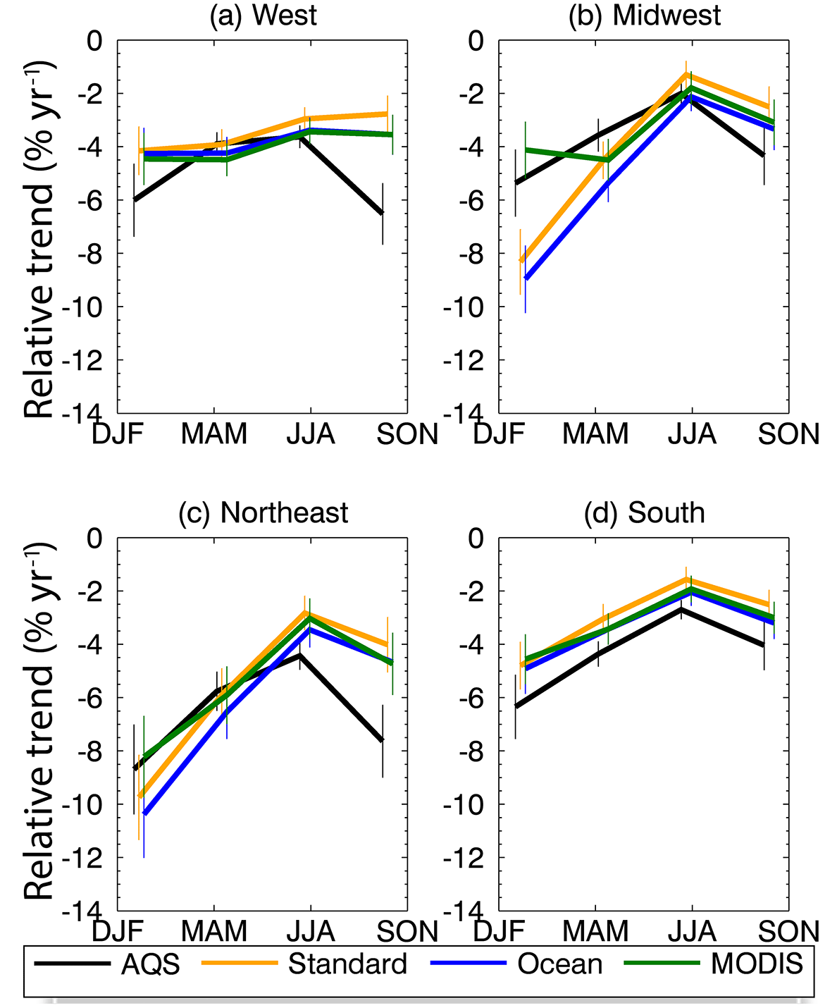
Figure 4Seasonal relative trends of NO2 calculated from the AQS in situ measurements (“AQS”, black line) and those derived from different OMI VCD data (“standard”, orange line; “ocean”, blue line; “MODIS”, green line). The error bars represent 95th-percentile confidence intervals.
3.1.1 Improvement due to ocean trend correction
After removing the ocean trend as discussed in Sect. 2.3.1, the OMI-based NO2 decreasing trends are more pronounced as shown in Fig. 4 (ocean version, blue line) by 0.1–0.9 % yr−1. The regional relative trends have different sensitivities to the ocean trend removal due to different tropospheric VCD levels. In general, the discrepancies between OMI-based and in situ trends are reduced except for the Midwest and the Northeast regions during DJF, which are already biased low. The averaged differences between OMI-based and in situ seasonal relative trends for the West, the Midwest, the Northeast, and the South regions are 1.2, −1.1, 0.4, and 1.0 % yr−1, respectively. Only in the Midwest region does removing the ocean trend enlarge the difference due to the large winter bias.
3.1.2 Improvement due to MODIS albedo update
The adoption of the up-to-date MODIS albedo (Sect. 2.3.2) greatly reduces the difference of relative trends in the Midwest during DJF from −3.6 % yr−1 (ocean version) to 1.3 % yr−1 (MODIS); the improvement of DJF trend difference is more moderate, from −1.7 to 0.5 % (Fig. 4). There are no significant changes of the comparisons in other regions or other seasons. Figure 5 shows the albedo seasonal relative trends for the four regions coincident with AQS in situ NO2 data. The OMI DOMINO v2 product incorporates a climatology albedo dataset (Kleipool et al., 2008) with snow/ice albedo adjustment, in which the albedo value is reset to be 0.6 if snow/ice is reported in the NASA Near-real-time Ice and Snow Extent (NISE) dataset (Boersma et al., 2011). The climatology albedo data have no trends. Thus, the trends of albedo from the DOMINO v2 product mainly originate from the yearly variation of NISE-detected snow/ice and to a lesser extent the OMI sampling variation. The noticeable seasonal trend of the OMI DOMINO v2 albedo dataset is the 3.9 % yr−1 increase in DJF of the Midwest and a smaller DJF increase (1.0 %) of the Northeast. In contrast, the MODIS albedo dataset exhibits a smaller positive DJF trend (0.8 % yr−1), 3.1 % yr−1 less than the trend from DOMINO v2, in the Midwest and a small negative DJF trend (−0.8 %) in the Northeast. These differences suggest that using a fixed snow/ice albedo and climatology albedo data is inadequate. The comparison to the AQS data shows that the MODIS albedo update leads to better agreement between satellite and in suit trends in winter in these regions (Fig. 4).

Figure 5Seasonal relative albedo trends of OMI (black line) and MODIS (red line) surface reflectance products, coincident with AQS in situ data used in Fig. 6. The error bars represent 95th-percentile confidence intervals.
3.1.3 Comparison after lightning event filter
As discussed in Sect. 2.3.3, lightning NOx affects the retrievals of satellite tropospheric NO2 VCDs and NO2 vertical mixing. Figure 6 shows that the lightning filter significantly reduces the difference between the OMI-based relative trend and that of the AQS data by 0.5–1.4 % yr−1 in the Northeast and 0.9–1.3 % yr−1 in the South. As a result, the seasonal trend differences are within 0.9 % yr−1 in these two regions except during SON. The Northeast is affected by the lightning filter due to lightning in this region and transport of lightning NOx from the South (Sect. 2.3.3). The lightning filter has little effect on the West and the Midwest. While lightning NOx can be significant during the monsoon season in some regions of the West (Fig. 3), the average tropospheric NO2 VCDs are usually < 1 × 10¹⁵ molecules cm−2, and lightning-affected regions are therefore excluded in trend analysis.
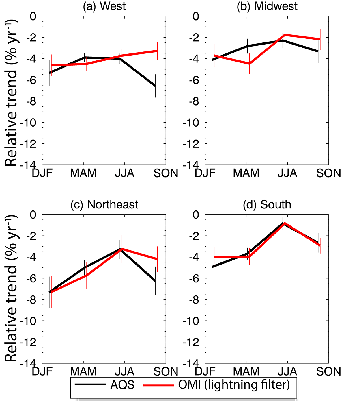
Figure 6Seasonal relative trends of NO2 calculated from the AQS in situ measurements (“AQS”, black line) and those derived from OMI data after applying the lightning filter (“OMI (lightning filter)”, red line). The error bars represent 95th-percentile confidence intervals. The coincident data points are less than those used in Fig. 4, and therefore the AQS trends are not the same.
Table 1Annual relative trends calculated with coincident data and all available data. The 95th-percentile confidence intervals from Mann–Kendall method are also listed.
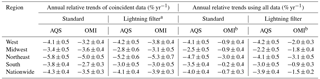
a These data include the three data processing procedures of this study, namely, ocean trend correction, MODIS albedo update, and lightning filter screening. b The spatial coverage is shown in Fig. 1.
The effect of the lightning filter (Fig. 6) cannot be shown in Fig. 4 because the coincident OMI and AQS data points are fewer after applying the lightning filter. We examine the improvements of ocean trend removal, MODIS albedo update, and data screening with the lightning filter by comparing the differences of different OMI-based seasonal relative trends from the AQS in situ trends in Fig. 7. The previously discussed improvements such as OMI albedo update for the Midwest and the Northeast during DJF are shown. By subtracting the AQS trends, we can now find clear improvements of the lightning filter for the South and the Northeast. There remains seasonal variation of OMI-based trend biases relative to in situ data, but the discrepancies of the annual trends after the three discussed procedures are relatively small at 0.3, −0.3, −0.1, and 0.0 % yr−1, in the West, the Midwest, the Northeast, and the South regions (Fig. 1), respectively. The remaining seasonal difference of the trends reflects in part the nonlinear photochemistry (Gu et al., 2013), the effects of NOx emission changes on NO2 retrievals (Lamsal et al., 2015), different spatial coverages of the two measurements, and the inherent difference between trends of NO2 tropospheric VCDs and surface concentrations.
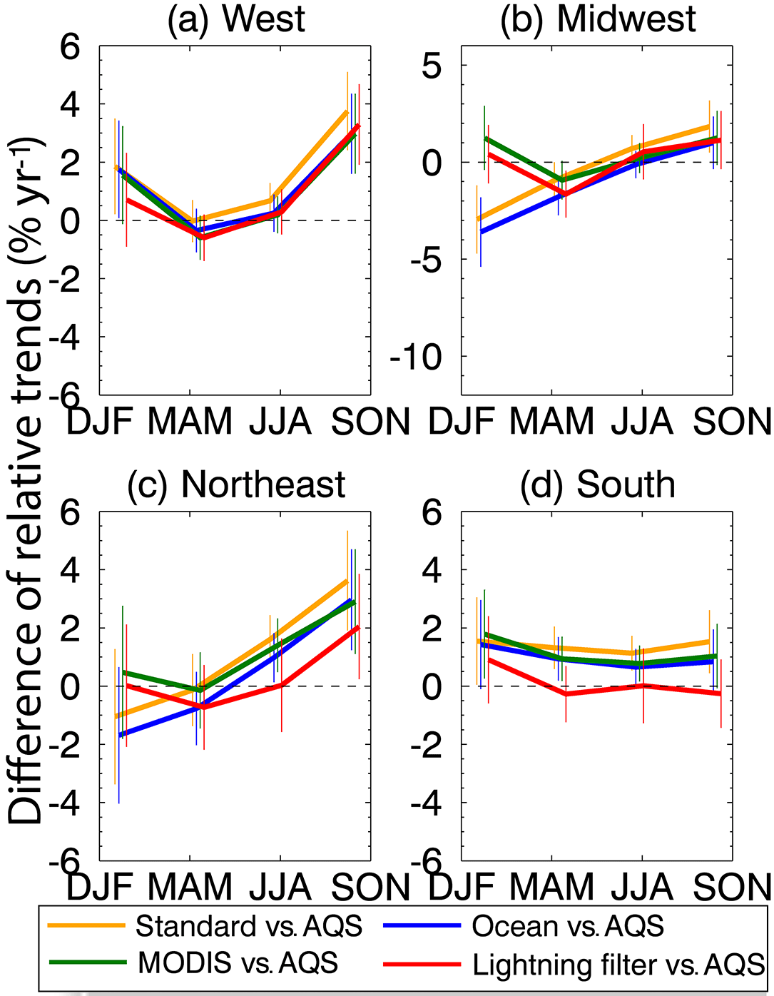
Figure 7Seasonal differences of OMI-based relative trends from those computed from AQS in situ data. The error bars represent 95th-percentile confidence intervals. The relative trends are shown in Figs. 4 and 6. The figure legends are the same as in Figs. 4 and 6 but with the AQS trends subtracted from the OMI-based trends.
3.2 OMI-based NO2 trends
Table 1 summarizes the regional annual trends of coincident AQS in situ and OMI data. The standard OMI data (following the DOMINO v2 algorithm) tend to show less NO2 reduction than AQS data. After applying the three data processing procedures discussed in the previous section to the OMI data, the agreement with the AQS trends is within the uncertainties of the trends. While lightning NOx is part of OMI NO2 observations, we treat the influence of lightning on the OMI tropospheric VCD trend as a bias for comparison purposes in this study. Table 1 shows the effects of data sampling when both AQS and OMI data are analyzed and when the lightning filter is applied.
Without the lightning filter, AQS decreasing trends are stronger than the decreasing trends of OMI data (Fig. 7). The lightning trend in the NLDN data is unclear due in part to the changing instrument sensitivity (Koshak et al., 2015). If lightning NOx is not accounted for in OMI retrieval, tropospheric NO2 VCDs are overestimated. On the other hand, lightning accompanies low-pressure systems which mix the atmosphere vertically and tend to reduce surface NO2 concentrations when anthropogenic emissions are high, such as urban and suburban regions. Therefore, lightning has opposite effects on surface and satellite trends. The low-pressure dilution effect on surface NO2 concentrations depends on anthropogenic emissions (since the end point of dilution is the background NO2 value). Therefore, the weaker decreasing surface trends likely reflect a reduction of the low-pressure dilution effect. Similarly, as anthropogenic emissions decrease, the positive bias of tropospheric VCDs due to lightning NOx becomes larger, likely resulting in weaker decreasing trends. We consider the lightning effects on surface NO2 trends to be mostly meteorologically driven not by lightning NOx directly (e.g., Ott et al., 2010; Luo et al., 2017), and hence the filtered OMI NO2 data are likely closer to emission-related concentration changes.
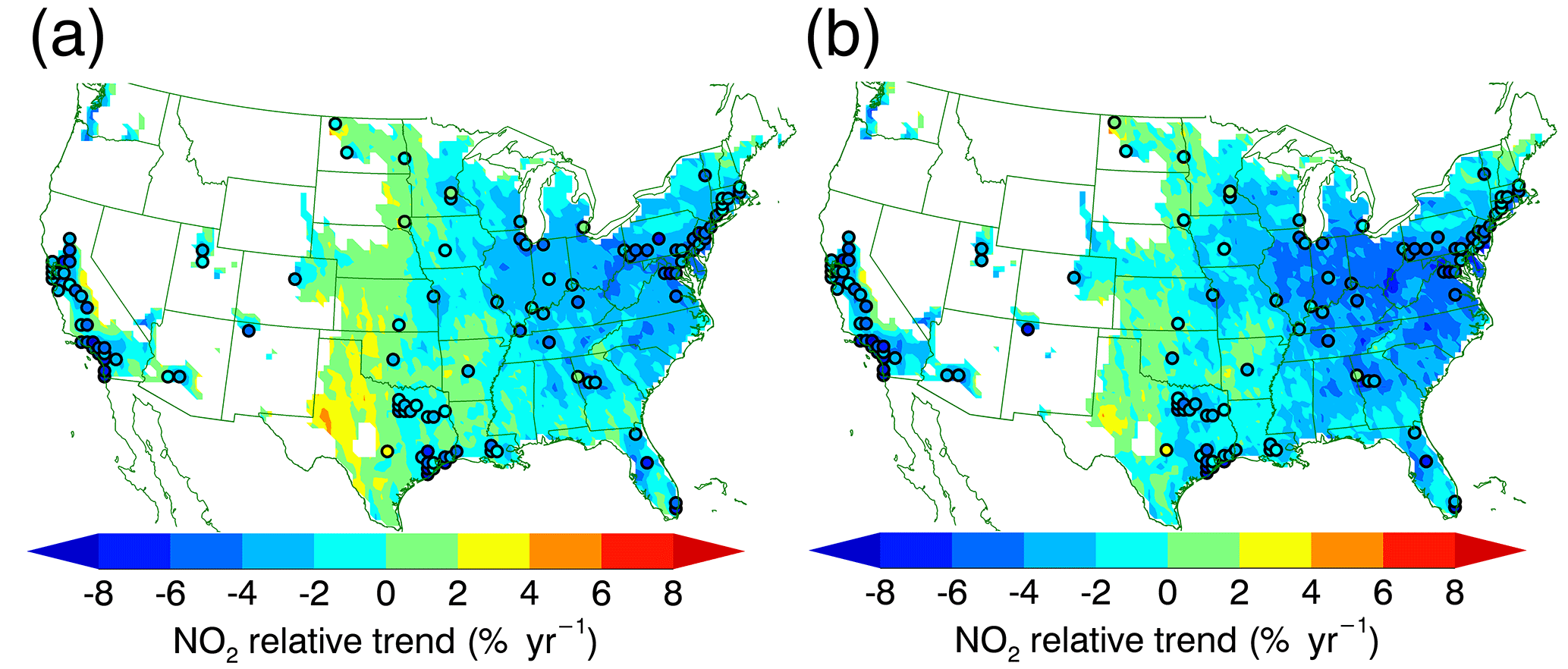
Figure 8Annual relative trends of OMI-based NO2 for “standard” (a) and for “lightning filter” (b) as the colored background. Black-bordered circles indicate corresponding AQS NO2 trends. Grid cells with 2005–2014 mean NO2 VCDs < 1 × 10¹⁵ molecules cm−2 are excluded in the analysis and are shown in white.
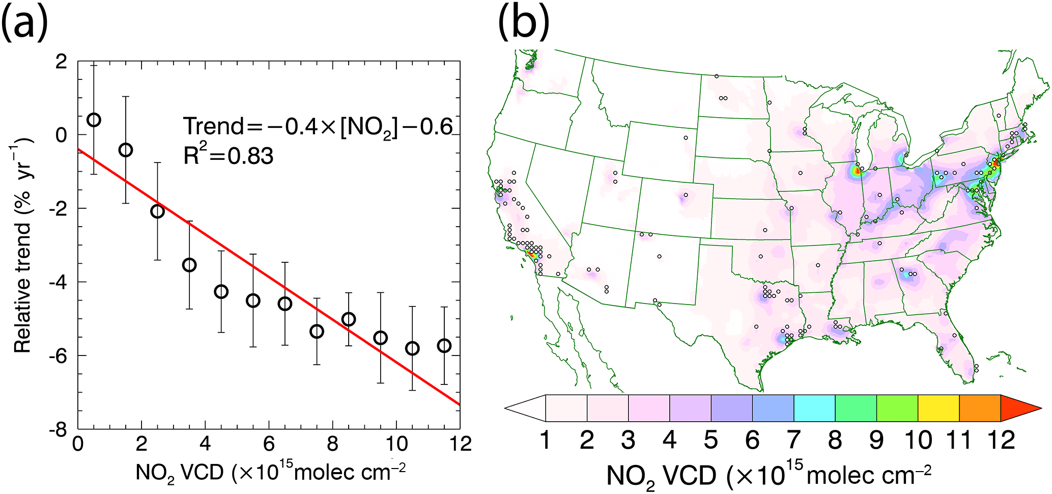
Figure 9(a) The “lightning filter” OMI-based NO2 relative trend as a function 2005–2014-averaged OMI tropospheric NO2 VCD binned every 1 × 10¹⁵ molec cm2. The error bars represent 95th-percentile confidence intervals. The red line shows a least-squares regression. (b) The distribution of 2005–2014-averaged OMI tropospheric NO2 VCD. Black-bordered circles represent AQS sites. The OMI tropospheric NO2 data (“lightning filter”) are used.
The AQS in situ NO2 annual relative trends (coincident with OMI data with the lightning filter) are most significant in the Northeast (−5.2 ± 0.6 % yr−1) and the West (−4.2 ± 0.5 % yr−1), followed by the South (−3.0 ± 0.5 % yr−1) and the Midwest (−2.8 ± 0.6 % yr−1) regions. The nationwide annual trend is −4.1 ± 0.4 % yr−1, which is consistent with the previous studies (Lamsal et al., 2015; Lu et al., 2015; Tong et al., 2015; de Foy et al., 2016b; Duncan et al., 2016; Krotkov et al., 2016). The significant NO2 reductions result from updated technologies and strict regulations (Krotkov et al., 2016). The OMI-based NO2 trends with the discussed procedures (coincident with AQS data) show similar reduction rates in the West (−3.8 ± 0.4 % yr−1), the Midwest (−3.1 ± 0.5 % yr−1), the Northeast (−5.3 ± 0.7 % yr−1), and the South (−3.0 ± 0.5 % yr−1) regions. The nationwide annual trend is −3.9 ± 0.3 % yr−1.
One advantage of satellite observations over a surface monitoring network is spatial coverage. The processed OMI data (lightning filter) coincident with the AQS data show a national annual trend of −3.9 ± 0.3 % yr−1, similar to the AQS in situ trend of −4.1 ± 0.4 % yr−1. Using all data available (Fig. 8, Table 1), the OMI data (lightning filter) show a much lower trend of −1.5 ± 0.2 % yr−1, about half of the AQS trend (−3.9 ± 0.4 % yr−1). Figure 9 shows that the AQS sites, which are mostly urban and suburban sites, tend to be located in regions with high tropospheric NO2 VCDs. The OMI decreasing trend is a function of tropospheric NO2 VCDs, increasing from 0 to −6 % yr−1 (Fig. 9). The national annual trend is close to the value of clean regions, which contribute much more than polluted regions. The larger decrease near the anthropogenic source regions reflects in part the nonlinear photochemistry (Gu et al., 2013) and in part a stronger influence of NOx sources such as soils in rural regions.
Using data from the DOMINO v2 algorithm, we find that the computed OMI-based seasonal NO2 (relative) trends underestimate the decreasing trends of the EPA AQS data by up to 3.7 % yr−1. While lightning NOx is part of OMI NO2 observations, we treat the influence of lightning on the OMI tropospheric VCD trend as a bias for comparison purposes in this study. Furthermore, lightning NOx effects need to be removed when using satellite observations to understand the effects of changing anthropogenic emissions.
In this study, we show that removing the background ocean trend, adopting MODIS albedo data (with better temporospatial resolutions and characterization of snow/ice), and excluding lightning influences can bring OMI tropospheric NO2 VCD trends in close agreement (within 0.3 % yr−1) with those of the AQS data. Among the corrections, the background ocean trend removal is not as significant as the latter two. Since the origin of this trend is not yet clear, the ocean trend removal method may need updates in future studies. The remaining differences may result from the inherent differences between trends of NO2 tropospheric VCDs and surface concentrations, different spatial sampling of the measurements, chemical nonlinearity, and tropospheric NO2 profile changes. The largest effects of the MODIS albedo update are in winter in the Midwest and Northeast, and those of lightning filter are in the South and the Northeast. After these data processing procedures are applied, the derived OMI-based annual regional NO2 trends change by a factor of > 2 for the South, the Midwest, and the West, and seasonal changes can be even larger. We derive OMI-based NO2 regional annual relative trends using all available data for the West (−2.0 % ± 0.3 yr−1), the Midwest (−1.8 % ± 0.4 yr−1), the Northeast (−3.1 % ± 0.5 yr−1), and the South (−0.9 % ± 0.3 yr−1).
The national annual trend of the processed OMI data is −1.5 ± 0.2 % yr−1, about half of the AQS trend (−3.9 ± 0.4 % yr−1). It reflects that the AQS sites are mostly located in the urban and suburban regions, where OMI data show much larger decreasing trends (up to −6 % yr−1) than rural regions (down to 0 % yr−1). The reasons for the dependence of OMI-derived trends on tropospheric NO2 VCDs and the seasonal/regional trend differences are still not completely understood. Further studies are necessary to improve our understanding of these trends. The observation-based lightning filter implemented in this study is preliminary. Incorporating chemical transport modeling may improve this filter. Moreover, the results presented here represent an alternative and indirect way to assess the importance of lightning NOx for National Climate Assessment (NCA) analyses described in Koshak et al. (2015) and Koshak (2017). Inversion studies (e.g., Zhao and Wang, 2009; Gu et al., 2013, 2014, 2016) will be needed to quantify the emission and AMF changes corresponding to the OMI tropospheric NO2 VCD trends.
The datasets used in this research have been obtained online as follows:
-
DOMINO v2 NO2 retrievals: http://www.temis.nl/airpollution/no2.html (last access: January 2016; Boersma et al., 2011).
-
EPA AQS NO2 data: US Environmental Protection Agency. Air Quality System Data Mart (internet database) available at: http://www.epa.gov/ttn/airs/aqsdatamart (last access: January 2016).
-
NLDN lightning data: https://lightning.nsstc.nasa.gov/data/data_nldn.html (last access: January 2016; Cummins et al., 2016).
-
MODIS MCD43B3 data: https://lpdaac.usgs.gov (LP DAAC, 2016).
The supplement related to this article is available online at: https://doi.org/10.5194/amt-11-3955-2018-supplement.
The authors declare that they have no conflict of interest.
This work was supported by the NASA Atmospheric Composition Modeling and Analysis Program (ACMAP) and the NASA Climate
Indicators and Data Products for Future National Climate Assessments
(NNH14ZDA001N-INCA). We acknowledge data sources, including DOMINO v2 OMI data
from KNMI, MODIS data from NASA, and EPA AQS NO2 data from EPA. In
addition, the authors gratefully acknowledge Vaisala Inc. for providing the
NLDN data used in this study. K. Folkert Boersma acknowledges funding from
the EU FP7 project QA4ECV (grant no. 607405).
Edited by: Andreas Richter
Reviewed by: two anonymous referees
Bey, I., Jacob, D. J., Yantosca, R. M., Logan, J. A., Field, B. D., Fiore, A. M., Li, Q. B., Liu, H. G. Y., Mickley, L. J., and Schultz, M. G.: Global modeling of tropospheric chemistry with assimilated meteorology: Model description and evaluation, J. Geophys. Res.-Atmos., 106, 23073–23095, https://doi.org/10.1029/2001jd000807, 2001.
Boersma, K. F., Eskes, H. J., and Brinksma, E. J.: Error analysis for tropospheric NO2 retrieval from space, J. Geophys. Res.-Atmos., 109, D04311, https://doi.org/10.1029/2003JD003962, 2004.
Boersma, K. F., Eskes, H. J., Dirksen, R. J., van der A, R. J., Veefkind, J. P., Stammes, P., Huijnen, V., Kleipool, Q. L., Sneep, M., Claas, J., Leitão, J., Richter, A., Zhou, Y., and Brunner, D.: An improved tropospheric NO2 column retrieval algorithm for the Ozone Monitoring Instrument, Atmos. Meas. Tech., 4, 1905–1928, https://doi.org/10.5194/amt-4-1905-2011, 2011.
Bucsela, E. J., Pickering, K. E., Huntemann, T. L., Cohen, R. C., Perring, A., Gleason, J. F., Blakeslee, R. J., Albrecht, R. I., Holzworth, R., Cipriani, J. P., Vargas-Navarro, D., Mora-Segura, I., Pacheco-Hernández, A., and Laporte-Molina, S.: Lightning-generated NOx seen by the Ozone Monitoring Instrument during NASA's Tropical Composition, Cloud and Climate Coupling Experiment (TC4), J. Geophys. Res.-Atmos., 115, D00J10, https://doi.org/10.1029/2009JD013118, 2010.
Castellanos, P. and Boersma, K. F.: Reductions in nitrogen oxides over Europe driven by environmental policy and economic recession, Sci. Rep., 2, 265, https://doi.org/10.1038/srep00265, 2012.
Cheng, Y., Wang, Y., Zhang, Y., Chen, G., Crawford, J. H., Kleb, M. M., Diskin, G. S., and Weinheimer, A. J.: Large biogenic contribution to boundary layer O3-CO regression slope in summer, Geophys. Res. Lett., 44, 7061–7068, https://doi.org/10.1002/2017GL074405, 2017.
Choi, Y., Wang, Y., Zeng, T., Martin, R. V., Kurosu, T. P., and Chance, K.: Evidence of lightning NOx and convective transport of pollutants in satellite observations over North America, Geophys. Res. Lett., 32, L02805, https://doi.org/10.1029/2004GL021436, 2005.
Choi, Y., Wang, Y., Zeng, T., Cunnold, D., Yang, E.-S., Martin, R., Chance, K., Thouret, V., and Edgerton, E.: Springtime transitions of NO2, CO, and O3 over North America: Model evaluation and analysis, J. Geophys. Res.-Atmos., 113, D20311, https://doi.org/10.1029/2007JD009632, 2008a.
Choi, Y., Wang, Y., Yang, Q., Cunnold, D., Zeng, T., Shim, C., Luo, M., Eldering, A., Bucsela, E., and Gleason, J.: Spring to summer northward migration of high O3 over the western North Atlantic, Geophys. Res. Lett., 35, L04818, https://doi.org/10.1029/2007GL032276, 2008b.
Cui, Y., Lin, J., Song, C., Liu, M., Yan, Y., Xu, Y., and Huang, B.: Rapid growth in nitrogen dioxide pollution over Western China, 2005–2013, Atmos. Chem. Phys., 16, 6207–6221, https://doi.org/10.5194/acp-16-6207-2016, 2016.
Cummins, K. L. and Murphy, M. J.: An Overview of Lightning Locating Systems: History, Techniques, and Data Uses, With an In-Depth Look at the U.S. NLDN, IEEE T. Electromagn. C., 51, 499–518, https://doi.org/10.1109/TEMC.2009.2023450, 2009.
Cummins, K. L., Burnett, R. O., Hiscox, W. L., and Pifer, A. E.: Line reliability and fault analysis using the National lightning detection network, Preprints, Precise Measurements in Power Conference, 27–29 October 1993, Arlington, VA, USA, 1993.
de Foy, B., Lu, Z., and Streets, D. G.: Satellite NO2 retrievals suggest China has exceeded its NOx reduction goals from the twelfth Five-Year Plan, Sci. Rep., 6, 35912, https://doi.org/10.1038/srep35912, 2016a.
de Foy, B., Lu, Z., and Streets, D. G.: Impacts of control strategies, the Great Recession and weekday variations on NO2 columns above North American cities, Atmos. Environ., 138, 74–86, https://doi.org/10.1016/j.atmosenv.2016.04.038, 2016b.
Demerjian, K. L.: A review of national monitoring networks in North America, Atmos. Environ., 34, 1861–1884, https://doi.org/10.1016/S1352-2310(99)00452-5, 2000.
Dirksen, R. J., Boersma, K. F., Eskes, H. J., Ionov, D. V., Bucsela, E. J., Levelt, P. F., and Kelder, H. M.: Evaluation of stratospheric NO2 retrieved from the Ozone Monitoring Instrument: Intercomparison, diurnal cycle, and trending, J. Geophys. Res.-Atmos., 116, D08305, https://doi.org/10.1029/2010JD014943, 2011.
Duncan, B. N., Yoshida, Y., de Foy, B., Lamsal, L. N., Streets, D. G., Lu, Z. F., Pickering, K. E., and Krotkov, N. A.: The observed response of Ozone Monitoring Instrument (OMI) NO2 columns to NOx emission controls on power plants in the United States: 2005–2011, Atmos. Environ., 81, 102–111, https://doi.org/10.1016/j.atmosenv.2013.08.068, 2013.
Duncan, B. N., Lamsal, L. N., Thompson, A. M., Yoshida, Y., Lu, Z., Streets, D. G., Hurwitz, M. M., and Pickering, K. E.: A space-based, high-resolution view of notable changes in urban NOx pollution around the world (2005–2014), J. Geophys. Res.-Atmos., 121, 976–996, https://doi.org/10.1002/2015JD024121, 2016.
Eskes, H. J. and Boersma, K. F.: Averaging kernels for DOAS total-column satellite retrievals, Atmos. Chem. Phys., 3, 1285–1291, https://doi.org/10.5194/acp-3-1285-2003, 2003.
Gu, D., Wang, Y., Smeltzer, C., and Liu, Z.: Reduction in NOx Emission Trends over China: Regional and Seasonal Variations, Environ. Sci. Technol., 47, 12912–12919, https://doi.org/10.1021/es401727e, 2013.
Gu, D., Wang, Y., Smeltzer, C., and Boersma, K. F.: Anthropogenic emissions of NOx over China: Reconciling the difference of inverse modeling results using GOME-2 and OMI measurements, J. Geophys. Res.-Atmos., 119, 7732–7740, https://doi.org/10.1002/2014JD021644, 2014.
Gu, D., Wang, Y., Yin, R., Zhang, Y., and Smeltzer, C.: Inverse modelling of NOx emissions over eastern China: uncertainties due to chemical non-linearity, Atmos. Meas. Tech., 9, 5193–5201, https://doi.org/10.5194/amt-9-5193-2016, 2016.
Guenther, A. B., Jiang, X., Heald, C. L., Sakulyanontvittaya, T., Duhl, T., Emmons, L. K., and Wang, X.: The Model of Emissions of Gases and Aerosols from Nature version 2.1 (MEGAN2.1): an extended and updated framework for modeling biogenic emissions, Geosci. Model Dev., 5, 1471–1492, https://doi.org/10.5194/gmd-5-1471-2012, 2012.
Heckel, A., Kim, S.-W., Frost, G. J., Richter, A., Trainer, M., and Burrows, J. P.: Influence of low spatial resolution a priori data on tropospheric NO2 satellite retrievals, Atmos. Meas. Tech., 4, 1805–1820, https://doi.org/10.5194/amt-4-1805-2011, 2011.
Kain, J. S. and Fritsch, J. M.: Convective Parameterization for Mesoscale Models: The Kain-Fritsch Scheme, in: The Representation of Cumulus Convection in Numerical Models, edited by: Emanuel, K. A., and Raymond, D. J., Am. Meteorol. Soc., Boston, MA, USA, 165–170, 1993.
Kendall, M. G.: Rank correlation methods, Rank correlation methods, Griffin, Oxford, UK, 1948.
Kleipool, Q. L., Dobber, M. R., de Haan, J. F., and Levelt, P. F.: Earth surface reflectance climatology from 3 years of OMI data, J. Geophys. Res.-Atmos., 113, D18308, https://doi.org/10.1029/2008JD010290, 2008.
Koshak, W. J.: Lightning NOx estimates from space-based lightning imagers, 16th Annual Community Modeling and Analysis System (CMAS) Conference, 23–25 October 2017, Chapel Hill, NC, USA, 2017.
Koshak, W. J., Cummins, K. L., Buechler, D. E., Vant-Hull, B., Blakeslee, R. J., Williams, E. R., and Peterson, H. S.: Variability of CONUS Lightning in 2003–12 and Associated Impacts, J. Appl. Meteorol. Clim., 54, 15–41, https://doi.org/10.1175/jamc-d-14-0072.1, 2015.
Krotkov, N. A., McLinden, C. A., Li, C., Lamsal, L. N., Celarier, E. A., Marchenko, S. V., Swartz, W. H., Bucsela, E. J., Joiner, J., Duncan, B. N., Boersma, K. F., Veefkind, J. P., Levelt, P. F., Fioletov, V. E., Dickerson, R. R., He, H., Lu, Z., and Streets, D. G.: Aura OMI observations of regional SO2 and NO2 pollution changes from 2005 to 2015, Atmos. Chem. Phys., 16, 4605–4629, https://doi.org/10.5194/acp-16-4605-2016, 2016.
Lamsal, L. N., Martin, R. V., van Donkelaar, A., Steinbacher, M., Celarier, E. A., Bucsela, E., Dunlea, E. J., and Pinto, J. P.: Ground-level nitrogen dioxide concentrations inferred from the satellite-borne Ozone Monitoring Instrument, J. Geophys. Res.-Atmos., 113, D16308, https://doi.org/10.1029/2007JD009235, 2008.
Lamsal, L. N., Martin, R. V., van Donkelaar, A., Celarier, E. A., Bucsela, E. J., Boersma, K. F., Dirksen, R., Luo, C., and Wang, Y.: Indirect validation of tropospheric nitrogen dioxide retrieved from the OMI satellite instrument: Insight into the seasonal variation of nitrogen oxides at northern midlatitudes, J. Geophys. Res.-Atmos., 115, D05302, https://doi.org/10.1029/2009JD013351, 2010.
Lamsal, L. N., Krotkov, N. A., Celarier, E. A., Swartz, W. H., Pickering, K. E., Bucsela, E. J., Gleason, J. F., Martin, R. V., Philip, S., Irie, H., Cede, A., Herman, J., Weinheimer, A., Szykman, J. J., and Knepp, T. N.: Evaluation of OMI operational standard NO2 column retrievals using in situ and surface-based NO2 observations, Atmos. Chem. Phys., 14, 11587–11609, https://doi.org/10.5194/acp-14-11587-2014, 2014.
Lamsal, L. N., Duncan, B. N., Yoshida, Y., Krotkov, N. A., Pickering, K. E., Streets, D. G., and Lu, Z.: U.S. NO2 trends (2005–2013): EPA Air Quality System (AQS) data versus improved observations from the Ozone Monitoring Instrument (OMI), Atmos. Environ., 110, 130–143, https://doi.org/10.1016/j.atmosenv.2015.03.055, 2015.
Land Processes Distributed Active Archive Center (LP DAAC): MODIS/Terra+Aqua Albedo 16-Day L3 Global 1km SIN Grid V004, Sioux Falls, South Dakota, USA, U.S. Geological Survey, V003, available at: https://lpdaac.usgs.gov, last access: January 2016.
Laughner, J. L., Zare, A., and Cohen, R. C.: Effects of daily meteorology on the interpretation of space-based remote sensing of NO2, Atmos. Chem. Phys., 16, 15247–15264, https://doi.org/10.5194/acp-16-15247-2016, 2016.
Lin, J.-T. and McElroy, M. B.: Detection from space of a reduction in anthropogenic emissions of nitrogen oxides during the Chinese economic downturn, Atmos. Chem. Phys., 11, 8171–8188, https://doi.org/10.5194/acp-11-8171-2011, 2011.
Lin, J.-T., McElroy, M. B., and Boersma, K. F.: Constraint of anthropogenic NOx emissions in China from different sectors: a new methodology using multiple satellite retrievals, Atmos. Chem. Phys., 10, 63–78, https://doi.org/10.5194/acp-10-63-2010, 2010.
Lin, J.-T., Liu, Z., Zhang, Q., Liu, H., Mao, J., and Zhuang, G.: Modeling uncertainties for tropospheric nitrogen dioxide columns affecting satellite-based inverse modeling of nitrogen oxides emissions, Atmos. Chem. Phys., 12, 12255–12275, https://doi.org/10.5194/acp-12-12255-2012, 2012.
Lin, J.-T., Pan, D., and Zhang, R.: Trend and Interannual Variability of Chinese Air Pollution since 2000 in Association with Socioeconomic Development: A Brief Overview, Atmos. Ocean. Sci. Lett., 6, 84–89, https://doi.org/10.1080/16742834.2013.11447061, 2013.
Lin, J.-T., Martin, R. V., Boersma, K. F., Sneep, M., Stammes, P., Spurr, R., Wang, P., Van Roozendael, M., Clémer, K., and Irie, H.: Retrieving tropospheric nitrogen dioxide from the Ozone Monitoring Instrument: effects of aerosols, surface reflectance anisotropy, and vertical profile of nitrogen dioxide, Atmos. Chem. Phys., 14, 1441–1461, https://doi.org/10.5194/acp-14-1441-2014, 2014.
Lin, J.-T., Liu, M.-Y., Xin, J.-Y., Boersma, K. F., Spurr, R., Martin, R., and Zhang, Q.: Influence of aerosols and surface reflectance on satellite NO2 retrieval: seasonal and spatial characteristics and implications for NOx emission constraints, Atmos. Chem. Phys., 15, 11217–11241, https://doi.org/10.5194/acp-15-11217-2015, 2015.
Liu, F., Beirle, S., Zhang, Q., van der A, R. J., Zheng, B., Tong, D., and He, K.: NOx emission trends over Chinese cities estimated from OMI observations during 2005 to 2015, Atmos. Chem. Phys., 17, 9261–9275, https://doi.org/10.5194/acp-17-9261-2017, 2017.
Liu, Z., Wang, Y., Gu, D., Zhao, C., Huey, L. G., Stickel, R., Liao, J., Shao, M., Zhu, T., Zeng, L., Liu, S.-C., Chang, C.-C., Amoroso, A., and Costabile, F.: Evidence of Reactive Aromatics As a Major Source of Peroxy Acetyl Nitrate over China, Environ. Sci. Technol., 44, 7017–7022, https://doi.org/10.1021/es1007966, 2010.
Liu, Z., Wang, Y., Vrekoussis, M., Richter, A., Wittrock, F., Burrows, J. P., Shao, M., Chang, C.-C., Liu, S.-C., Wang, H., and Chen, C.: Exploring the missing source of glyoxal (CHOCHO) over China, Geophys. Res. Lett., 39, L10812, https://doi.org/10.1029/2012GL051645, 2012a.
Liu, Z., Wang, Y., Gu, D., Zhao, C., Huey, L. G., Stickel, R., Liao, J., Shao, M., Zhu, T., Zeng, L., Amoroso, A., Costabile, F., Chang, C.-C., and Liu, S.-C.: Summertime photochemistry during CAREBeijing-2007: ROx budgets and O3 formation, Atmos. Chem. Phys., 12, 7737–7752, https://doi.org/10.5194/acp-12-7737-2012, 2012b.
Lu, Z., Streets, D. G., de Foy, B., Lamsal, L. N., Duncan, B. N., and Xing, J.: Emissions of nitrogen oxides from US urban areas: estimation from Ozone Monitoring Instrument retrievals for 2005–2014, Atmos. Chem. Phys., 15, 10367–10383, https://doi.org/10.5194/acp-15-10367-2015, 2015.
Luo, C., Wang, Y., and Koshak, W. J.: Development of a self-consistent lightning NOx simulation in large-scale 3-D models, J. Geophys. Res.-Atmos., 122, 3141–3154, https://doi.org/10.1002/2016JD026225, 2017.
Mann, H. B.: Nonparametric Tests Against Trend, Econometrica, 13, 245–259, https://doi.org/10.2307/1907187, 1945.
Martin, R. V., Sauvage, B., Folkins, I., Sioris, C. E., Boone, C., Bernath, P., and Ziemke, J.: Space-based constraints on the production of nitric oxide by lightning, J. Geophys. Res.-Atmos., 112, D09309, https://doi.org/10.1029/2006JD007831, 2007.
Ott, L. E., Pickering, K. E., Stenchikov, G. L., Allen, D. J., DeCaria, A. J., Ridley, B., Lin, R.-F., Lang, S., and Tao, W.-K.: Production of lightning NOx and its vertical distribution calculated from three-dimensional cloud-scale chemical transport model simulations, J. Geophys. Res.-Atmos., 115, D04301, https://doi.org/10.1029/2009JD011880, 2010.
Pickering, K. E., Wang, Y., Tao, W.-K., Price, C., and Müller, J.-F.: Vertical distributions of lightning NOx for use in regional and global chemical transport models, J. Geophys. Res.-Atmos., 103, 31203–31216, https://doi.org/10.1029/98JD02651, 1998.
Rudlosky, S. D. and Fuelberg, H. E.: Pre- and Postupgrade Distributions of NLDN Reported Cloud-to-Ground Lightning Characteristics in the Contiguous United States, Mon. Weather Rev., 138, 3623–3633, https://doi.org/10.1175/2010mwr3283.1, 2010.
Russell, A. R., Perring, A. E., Valin, L. C., Bucsela, E. J., Browne, E. C., Wooldridge, P. J., and Cohen, R. C.: A high spatial resolution retrieval of NO2 column densities from OMI: method and evaluation, Atmos. Chem. Phys., 11, 8543–8554, https://doi.org/10.5194/acp-11-8543-2011, 2011.
Russell, A. R., Valin, L. C., and Cohen, R. C.: Trends in OMI NO2 observations over the United States: effects of emission control technology and the economic recession, Atmos. Chem. Phys., 12, 12197–12209, https://doi.org/10.5194/acp-12-12197-2012, 2012.
Saha, S., Moorthi, S., Pan, H.-L., Wu, X., Wang, J., Nadiga, S., Tripp, P., Kistler, R., Woollen, J., Behringer, D., Liu, H., Stokes, D., Grumbine, R., Gayno, G., Wang, J., Hou, Y.-T., Chuang, H.-Y., Juang, H.-M. H., Sela, J., Iredell, M., Treadon, R., Kleist, D., Van Delst, P., Keyser, D., Derber, J., Ek, M., Meng, J., Wei, H., Yang, R., Lord, S., Van Den Dool, H., Kumar, A., Wang, W., Long, C., Chelliah, M., Xue, Y., Huang, B., Schemm, J.-K., Ebisuzaki, W., Lin, R., Xie, P., Chen, M., Zhou, S., Higgins, W., Zou, C.-Z., Liu, Q., Chen, Y., Han, Y., Cucurull, L., Reynolds, R. W., Rutledge, G., and Goldberg, M.: The NCEP Climate Forecast System Reanalysis, B. Am. Meteorol. Soc., 91, 1015–1057, https://doi.org/10.1175/2010BAMS3001.1, 2010.
Schaaf, C. B., Gao, F., Strahler, A. H., Lucht, W., Li, X., Tsang, T., Strugnell, N. C., Zhang, X., Jin, Y., Muller, J.-P., Lewis, P., Barnsley, M., Hobson, P., Disney, M., Roberts, G., Dunderdale, M., Doll, C., d'Entremont, R. P., Hu, B., Liang, S., Privette, J. L., and Roy, D.: First operational BRDF, albedo nadir reflectance products from MODIS, Remote Sens. Environ., 83, 135–148, https://doi.org/10.1016/S0034-4257(02)00091-3, 2002.
Schenkeveld, V. M. E., Jaross, G., Marchenko, S., Haffner, D., Kleipool, Q. L., Rozemeijer, N. C., Veefkind, J. P., and Levelt, P. F.: In-flight performance of the Ozone Monitoring Instrument, Atmos. Meas. Tech., 10, 1957–1986, https://doi.org/10.5194/amt-10-1957-2017, 2017.
Tang, J., Zhang, A., and He, Z.: The earth surface reflectance retrieval by exploiting the synergy of TERRA and AQUA MODIS data, 2007 IEEE International Geoscience and Remote Sensing Symposium, 23–28 July 2007, Barcelona, Spain, 1697–1700, https://doi.org/10.1109/IGARSS.2007.4423144, 2007.
Tong, D. Q., Lamsal, L., Pan, L., Ding, C., Kim, H., Lee, P., Chai, T., Pickering, K. E., and Stajner, I.: Long-term NOx trends over large cities in the United States during the great recession: Comparison of satellite retrievals, ground observations, and emission inventories, Atmos. Environ., 107, 70–84, https://doi.org/10.1016/j.atmosenv.2015.01.035, 2015.
Yang, Q., Wang, Y., Zhao, C., Liu, Z., Gustafson, W. I., and Shao, M.: NOx Emission Reduction and its Effects on Ozone during the 2008 Olympic Games, Environ. Sci. Technol., 45, 6404–6410, https://doi.org/10.1021/es200675v, 2011.
Zara, M., Boersma, K. F., De Smedt, I., Richter, A., Peters, E., Van Geffen, J. H. G. M., Beirle, S., Wagner, T., Van Roozendael, M., Marchenko, S., Lamsal, L. N., and Eskes, H. J.: Improved slant column density retrieval of nitrogen dioxide and formaldehyde for OMI and GOME-2A from QA4ECV: intercomparison, uncertainty characterization, and trends, Atmos. Meas. Tech. Discuss., https://doi.org/10.5194/amt-2017-453, in review, 2018.
Zhang, R., Wang, Y., He, Q., Chen, L., Zhang, Y., Qu, H., Smeltzer, C., Li, J., Alvarado, L. M. A., Vrekoussis, M., Richter, A., Wittrock, F., and Burrows, J. P.: Enhanced trans-Himalaya pollution transport to the Tibetan Plateau by cut-off low systems, Atmos. Chem. Phys., 17, 3083–3095, https://doi.org/10.5194/acp-17-3083-2017, 2017.
Zhang, Y. and Wang, Y.: Climate-driven ground-level ozone extreme in the fall over the Southeast United States, P. Natl. Acad. Sci., 113, 10025-10030, https://doi.org/10.1073/pnas.1602563113, 2016.
Zhang, Y., Wang, Y., Chen, G., Smeltzer, C., Crawford, J., Olson, J., Szykman, J., Weinheimer, A. J., Knapp, D. J., Montzka, D. D., Wisthaler, A., Mikoviny, T., Fried, A., and Diskin, G.: Large vertical gradient of reactive nitrogen oxides in the boundary layer: Modeling analysis of DISCOVER-AQ 2011 observations, J. Geophys. Res.-Atmos., 121, 1922–1934, https://doi.org/10.1002/2015JD024203, 2016.
Zhao, C. and Wang, Y.: Assimilated inversion of NOx emissions over east Asia using OMI NO2 column measurements, Geophys. Res. Lett., 36, L06805, https://doi.org/10.1029/2008GL037123, 2009.
Zhao, C., Wang, Y., Choi, Y., and Zeng, T.: Summertime impact of convective transport and lightning NOx production over North America: modeling dependence on meteorological simulations, Atmos. Chem. Phys., 9, 4315–4327, https://doi.org/10.5194/acp-9-4315-2009, 2009.
Zhou, Y., Brunner, D., Boersma, K. F., Dirksen, R., and Wang, P.: An improved tropospheric NO2 retrieval for OMI observations in the vicinity of mountainous terrain, Atmos. Meas. Tech., 2, 401–416, https://doi.org/10.5194/amt-2-401-2009, 2009.