the Creative Commons Attribution 4.0 License.
the Creative Commons Attribution 4.0 License.
 | 08 Mar 2018
Raindrop fall velocities from an optical array probe and 2-D video disdrometer
Viswanathan Bringi
Merhala Thurai
Darrel Baumgardner
We report on fall speed measurements of raindrops in light-to-heavy rain events from two climatically different regimes (Greeley, Colorado, and Huntsville, Alabama) using the high-resolution (50 µm) Meteorological Particle Spectrometer (MPS) and a third-generation (170 µm resolution) 2-D video disdrometer (2DVD). To mitigate wind effects, especially for the small drops, both instruments were installed within a 2∕3-scale Double Fence Intercomparison Reference (DFIR) enclosure. Two cases involved light-to-moderate wind speeds/gusts while the third case was a tornadic supercell and several squall lines that passed over the site with high wind speeds/gusts. As a proxy for turbulent intensity, maximum wind speeds from 10 m height at the instrumented site recorded every 3 s were differenced with the 5 min average wind speeds and then squared. The fall speeds vs. size from 0.1 to 2 and >0.7 mm were derived from the MPS and the 2DVD, respectively. Consistency of fall speeds from the two instruments in the overlap region (0.7–2 mm) gave confidence in the data quality and processing methodologies. Our results indicate that under low turbulence, the mean fall speeds agree well with fits to the terminal velocity measured in the laboratory by Gunn and Kinzer from 100 µm up to precipitation sizes. The histograms of fall speeds for 0.5, 0.7, 1 and 1.5 mm sizes were examined in detail under the same conditions. The histogram shapes for the 1 and 1.5 mm sizes were symmetric and in good agreement between the two instruments with no evidence of skewness or of sub- or super-terminal fall speeds. The histograms of the smaller 0.5 and 0.7 mm drops from MPS, while generally symmetric, showed that occasional occurrences of sub- and super-terminal fall speeds could not be ruled out. In the supercell case, the very strong gusts and inferred high turbulence intensity caused a significant broadening of the fall speed distributions with negative skewness (for drops of 1.3, 2 and 3 mm). The mean fall speeds were also found to decrease nearly linearly with increasing turbulent intensity attaining values about 25–30 % less than the terminal velocity of Gunn–Kinzer, i.e., sub-terminal fall speeds.


Knowledge of the terminal fall speed of raindrops as a function of size is important in modeling collisional breakup and coalescence processes (e.g., List et al., 1987), in the radar-based estimation of rain rate, in retrieval of drop size distribution using Doppler spectra at vertical incidence (e.g., Sekhon and Srivastava, 1971) and in soil erosion studies (e.g., Rosewell, 1986). In these and other applications it is generally accepted that there is a unique fall speed ascribed to drops of a given mass or diameter and that it equals the terminal speed with adjustment for pressure (e.g., Beard, 1976). The terminal velocity measurements of Gunn and Kinzer (1949) under calm laboratory conditions and fits to their data (e.g., Atlas et al., 1973; Foote and du Toit, 1969; Beard and Pruppacher, 1969) are still considered the standard against which measurements using more modern optical instruments in natural rain are compared (Löffler-Mang and Joss, 2000; Barthazy et al., 2004; Schönhuber et al., 2008; Testik and Rahman, 2016; Yu et al., 2016). More recently, the broadening and skewness of the fall speed distributions of a given size (3 mm) in one intense rain event were attributed to mixed-mode amplitude oscillations (Thurai et al., 2013). Super- and sub-terminal fall speeds in intense rain shafts have been detected and attributed, respectively, to drop breakup fragments (sizes <0.5 mm) and high wind/gusts (sizes 1–2 mm) (Montero-Martinez et al., 2009; Larsen et al., 2014; Montero-Martinez and Garcia-Garcia, 2016). Thus, there is some evidence that raindrops may not fall at their terminal velocity except under calm conditions and that the concept of a fall speed distribution for a drop of given mass (or, diameter) might need to be considered, which is the topic of this paper. The implications are rather profound, especially for numerical modeling of collision-coalescence and breakup processes, which are important for shaping the drop size distribution.
The fall speeds and concentration of small drops (<1 mm) in natural rain are difficult to measure accurately given the poor resolution (>170 µm) of most optical disdrometers and/or sensitivity issues. While cloud imaging probes (with high resolution 25–50 µm) on aircraft have been used for many years, they generally cannot measure the fall speeds. A relatively new instrument, the Meteorological Particle Spectrometer (MPS), is a droplet imaging probe built by Droplet Measurements Technologies (DMT, Inc.) under contract from the US Weather Service and specifically designed for drizzle as small as 50 µm and raindrops up to 3 mm. This instrument in conjunction with a lower-resolution 2-D video disdrometer (2DVD; Schoenhuber et al., 2008) is used in this paper to measure fall speed distributions in natural rain.
This paper briefly describes the instruments used, presents fall speed measurements from two sites under relatively low wind conditions and one case from an unusual tornadic supercell with high winds and gusts, and ends with a brief discussion and summary of the results.
The principal instruments used in this study are the MPS and third-generation 2DVD, both located within a 2∕3-scale Double Fence Intercomparison Reference (DFIR; Rasmussen et al., 2012) wind shield. As reported in Notaros et al. (2016), the 2∕3-scale DFIR was effective in reducing the ambient wind speeds by nearly a factor of 2–3 based on data from outside and inside the fence. The flow field in and around the DFIR has been simulated by Theriault et al. (2015) assuming steady ambient winds. They found that depending on the wind direction relative to the octagonal fence, weak vertical motions could be generated above the sensor areas. For 5 m s−1 speeds, the motions could range between −0.4 (down draft) and 0.2 m s−1 (up draft).
The instrument setup was the same for the two sites (Greeley, Colorado, and Huntsville, Alabama). Huntsville has a very different climate from Greeley, and its altitude is 212 m m.s.l. as compared with 1.4 km m.s.l. for Greeley. According to the Köppen–Trewartha climate classification system (Trewartha and Horn, 1980), this labels Greeley as a semiarid-type climate, whereas Huntsville is a humid subtropical-type climate (Belda et al., 2014).
The MPS is an optical array probe (OAP) that uses the technique introduced by Knollenberg (1970, 1976, 1981) and measures drop diameter in the range from 0.05 to 3.1 mm. A 64-element photodiode array is illuminated with a 660 nm collimated laser beam. Droplets passing through the laser cast a shadow on the array and the decrease in light intensity on the diodes is monitored with the signal processing electronics. A two-dimensional image is captured by recording the light level of each diode during the period that the array is shadowed. The fall velocity is derived using two methods. One uses the same approach as described by Montero-Martinez et al. (2009), in which the fall velocity is calculated from the product of the true air speed clock and ratio of the image height to width. Note that “width” is the horizontal dimension parallel to the array and “height” is along the vertical. The second method computes the fall velocity from the maximum horizontal dimension (spherical drop shape assumption) divided by the amount of time that the image is on the array, a time measured with a 2 MHz clock. In order to be comparable to the results of Montero-Martinez et al. (2009), their approach is implemented here for sizes >250 µm. The fall velocity of smaller, slower-moving droplets is measured using the second technique.
The limitations and uncertainties associated with OAP measurements have been well documented (Korolev et al., 1991, 1998; Baumgardner et al., 2016). There are a number of potential artifacts that arise when making measurements with optical array probes (Baumgardner et al., 2016): droplet breakup on the probe tips that form satellite droplets, multiple droplets imaged simultaneously and out-of-focus drops whose images are usually larger than the actual drop (Korolev, 2007). The measured images have been analyzed to remove satellite droplets whose interarrival times are usually too short to be natural drops; multiple drops are detected by shape analysis and removed, and out-of-focus drops are detected and size corrected using the technique described by (Korolev, 2007). The sizing and fall speed errors primarily depend on the digitization error (±25 µm). The fall speed accuracy according to the manufacturer (DMT) is <10 % for 0.25 mm and <1 % for sizes greater than 1 mm, limited primarily by the accuracy in droplet sizing.
The third-generation 2DVD is described in detail by Schoenhuber et al. (2007, 2008) and its accuracy of size and fall speed measurement has been well documented (e.g., Thurai et al., 2007, 2009; Huang et al., 2008; Bernauer et al., 2015). Considering the horizontal pixel resolution of 170 µm and other factors (such as “mismatched” drops), the effective sizing range is D>0.7 mm. To clarify the mismatched drop problem: it is very difficult to match a drop detected in the top light-beam plane of the 2DVD to the corresponding drop in the bottom plane for tiny drops resulting in erroneous fall speeds. The fall velocity accuracy is determined primarily by the accuracy of calibrating the distance between the two orthogonal light “sheets” or planes and is <5 % for fall velocity <10 m s−1. In our application, we utilize the MPS for measurement of small drops with D<1.2 mm. The measurements from the MPS are compared with those from the 2DVD in the overlap region of D≈0.7–2.0 mm to ensure consistency of observations. The only fall velocity threshold used for the 2DVD is the lower limit set at 0.5 m s−1 in accordance with the manufacturer guidelines for rain measurements.
2.1 Fall speeds from Greeley, Colorado
We first consider a long duration (around 20 h) rain episode on 17 April 2015 which consisted of a wide variety of rain types/rates (mostly light stratiform <8 mm h−1) as described in Table 2 of Thurai et al. (2017). Two wind sensors at a height of 1 m were available to measure the winds outside and inside the DFIR. Average wind speeds were, respectively, <1.5 m s−1 inside the DFIR and <4 m s−1 outside with light gusts. These wind sensors were specific to the winter experiment described in Notaros et al. (2016) and were unavailable for the rain measurement campaign after May 2015.
Figure 1a shows the fall speeds vs. D from the 2DVD (shown as contoured frequency of occurrence), along with mean and ±1σ standard deviation from the MPS. Also shown is the fit of Foote and du Toit (1969) (henceforth FT fit) to the terminal fall speed measurements of Gunn and Kinzer (1949) at sea level and after applying altitude corrections (Beard, 1976) for the elevation of 1.4 km m.s.l. for Greeley. Panels b and c show the histogram of fall speeds for diameter intervals (0.5±0.1) and (1±0.1 mm) and (0.7±0.1) and (1.5±0.1 mm), respectively. Panel a demonstrates the excellent “visual” agreement between the two instruments in the overlap size range (0.7–2 mm), which is quantified in Table 1. However, the altitude-adjusted FT fit is slightly higher than the measured values as shown in Table 1. Notable in Fig. 1a is the remarkable agreement in mean fall speeds between the FT fit and the MPS for D<0.5 mm down to near the lower limit of the instrument (0.1 mm). Few measurements have been reported of fall speeds in this size range.
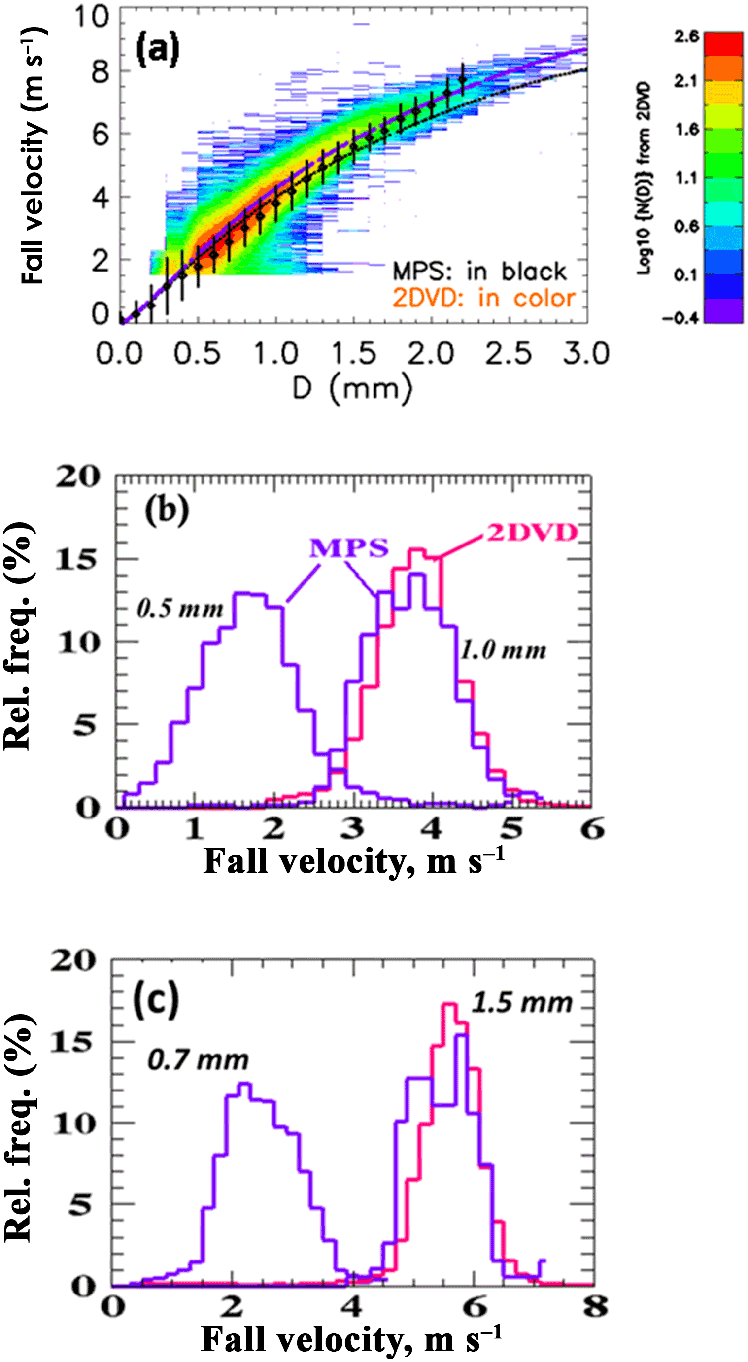
Figure 1(a) Fall velocity vs. diameter (D). The contoured frequency of occurrence from 2DVD data is shown in color (log scale). The mean fall velocity and ±1σ standard deviation bars are from MPS. The dark dashed line is from the fit to the laboratory data of Gunn and Kinzer (1949) and the purple line is the same except corrected for the altitude of Greeley, CO (1.4 km m.s.l.). (b) Relative frequency histograms of fall velocity for the 0.5±0.1 mm and 1±0.1 mm bins. (c) As in (b) but for the 0.7±0.1 mm and 1.5±0.1 mm bins.
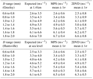
Table 1Expected fall velocities for various diameter intervals (bin width of 0.2 mm) from Foote and du Toit (1969) with altitude adjustment and the measured mean fall velocities with ±1σ (standard deviation).
The histograms in Fig. 1b and c show good agreement between 2DVD and MPS for 1 and 1.5 mm drop sizes, respectively, with respect to the mode, symmetry, spectral width and lack of skewness in the distributions. For the 1 mm size histogram, the mean is 3.8 m s−1 while the spectral width or standard deviation from MPS data is 0.6 m s−1. The corresponding coefficient of variation (ratio of standard deviation to mean) is 15.7 %. The finite bin width used (0.9–1.1 mm) causes a corresponding fall speed “spread” of around 0.6 m s−1, which is clearly a significant contributor to the measured coefficient of variation. Similar comments apply to the fall speed histogram for the 1.5 mm size shown in Fig. 1c. The definition of sub- or super-terminal fall speeds by Montero-Martinez et al. (2009) is based on fall speeds that are, respectively, less than 0.7 times the mean value or greater than 1.3 times the mean value (i.e., exceeding 30 % threshold on either side of the mean terminal fall speed). From examining the 1 mm size fall speed histogram there is negligible evidence of occurrences with fall speeds <2.66 m s−1 (sub) or >4.94 m s−1 (super). Similar comment also applies for the 1.5 mm size based on the corresponding histogram.
The histogram from MPS for the 0.5 mm sizes shows positive skewness with mean of 1.8 m s−1, spectral width of 0.65 m s−1 and corresponding coefficient of variation nearly doubling to 35 % (relative to the 1 mm size histogram). The finite bin width (0.4–0.6 mm) causes a corresponding fall speed “spread” of 0.4 m s−1, which contributes to the measured coefficient of variation. Nevertheless, it is not possible to rule out the low frequency of occurrence of sub- or super-terminal fall speeds that is less than 1.26 m s−1 or exceeding 2.34 m s−1, respectively, based on our data. Examination of the MPS-based fall speed histogram for the 0.7 mm size indicates negative skewness. As with the 0.5 mm drops it is not possible to rule out the occurrences of fall speeds <1.8 m s−1 or >3.4 m s−1, i.e., sub- or super-terminal fall speeds.
2.2 Fall speeds from Huntsville, Alabama
The first Huntsville event occurred on 11 April 2016 and consisted of precipitation associated with the mesoscale vortex of a developing squall line that moved across northern Alabama between 18:00 and 23:00 UTC and produced over 25 mm of rainfall in the Huntsville area. Figure 2a shows the ambient 10 m height wind speeds (3 s and 5 min averaged) recorded at the site. Maximum speeds were less than 5 m s−1 and wind gusts were light. As no direct in situ measurement of turbulence was available, we use the approach by Garrett and Yuter (2014), who estimate the difference between the maximum wind speed, or gust, which was sampled every 3 s, and the average wind speed derived from successive 5 min intervals. The estimated turbulent intensity is proportional to . Figure 2b shows the E values, which were small (maximum E<0.4 m2 s−2) and indicative of low turbulence. Also shown in Fig. 2b is the 2DVD-based time series of rainfall rate (R) averaged over 3 min; the maximum R is around 10 mm h−1.
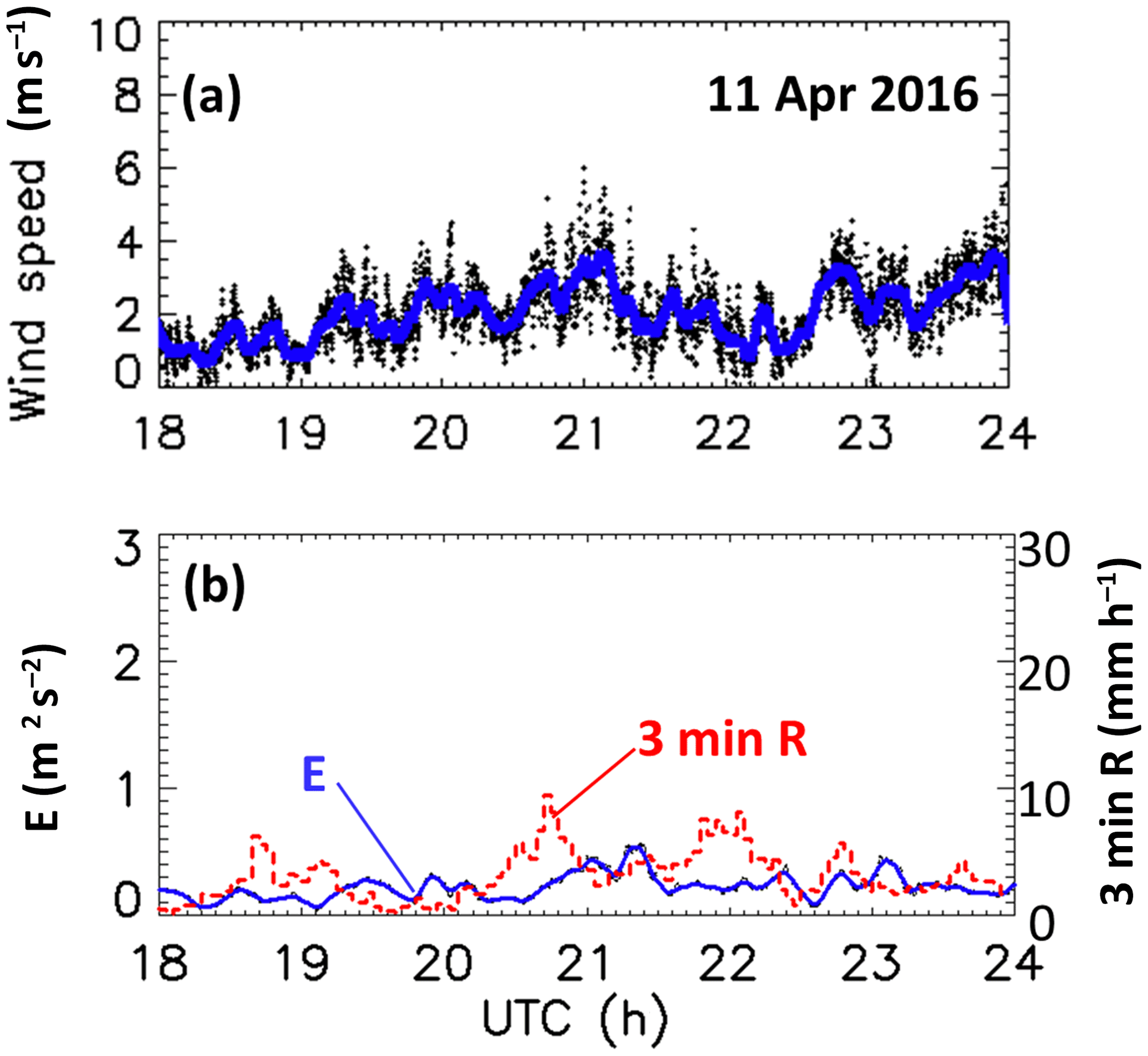
Figure 2(a) The 3 s raw and 5 min averaged wind speeds at 10 m height. (b) Turbulent intensity estimates E and 3 min averaged R.
Figure 3a shows the fall velocity vs. D comparison between the two instruments while panels b and c show the histograms for the 0.5 and 1 mm and 0.7 and 1.5 mm sizes, respectively. Similar to the Greeley event, the mean fall speed agreement between both instruments in the overlap region is excellent (see Table 1) and consistent with the FT fit to the Gunn–Kinzer laboratory data. As in Fig. 1a, the MPS data in Fig. 3a are in excellent agreement with FT fit for sizes <0.5 mm.
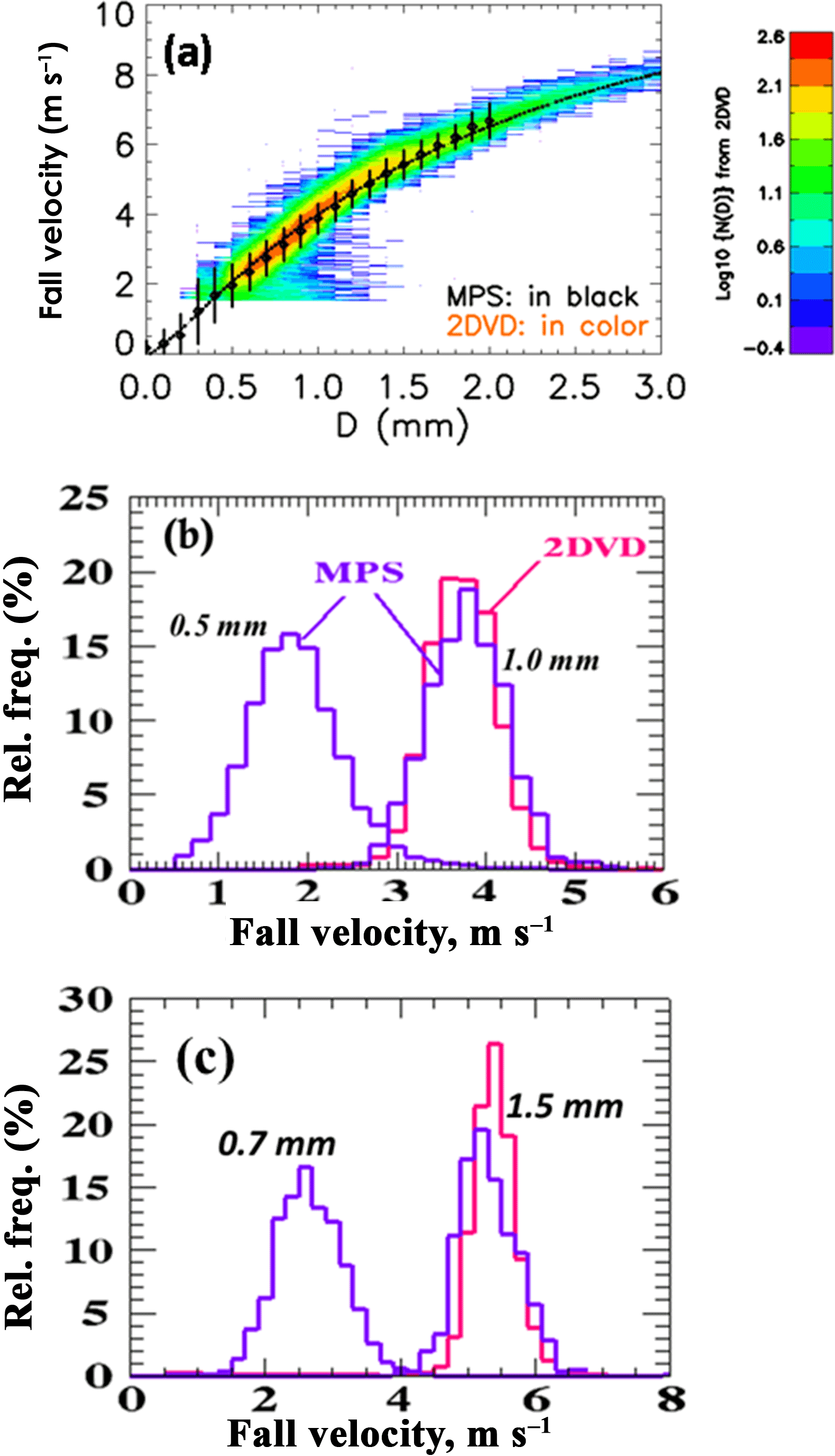
Figure 3(a) As in Fig. 1a except for 11 April 2016 event. The dashed line is fit to Gunn–Kinzer at sea level. (b, c) As in Fig. 1b and c but for 11 April 2016 event.
The 0.5 and 1 mm histogram shapes in Fig. 3b are quite similar to the Greeley case shown in Fig. 1b. The mean and SDs from the MPS data for the 0.5 and 1 mm bins are, respectively, [2±0.62] and [3.88±0.44] m s−1. The values for the 0.7 and 1.5 mm bins are, respectively, [2.6±0.6] and [5.4±0.4] m s−1. There is negligible evidence of sub- or super-terminal fall speed occurrences based on the 1 and 1.5 mm histograms. The comments made earlier with respect to Fig. 1b and c of the Greeley event for the 0.5 and 0.7 mm histograms are also applicable here; i.e., we cannot rule out the occasional occurrences of sub- or super-terminal fall speeds based on our data.
The second case considered is from 30 November 2016 wherein a supercell passed over the instrumented site from 03:00 to 03:30 UTC, producing about 15 min later a long-lived EF-2 tornado. Strong winds were recorded at the site, with 5 min averaged speeds reaching 10–12 m s−1 between 03:20 and 03:30 and E values in the range of 7–8 m2 s−2, indicating strong turbulence (Fig. 4a and b). The rain rates peaked at 70 mm h−1 during this time (Fig. 4b). About 3 h later several squall-line-type storm cells passed over the site from 07:00 to 09:00 UTC, again with strong winds but considerably lower E values 2–4 m2 s−2 and maximum R of 80 mm h−1. After 10:00 UTC the E values were much smaller (<0.5 m2 s−2), indicating calm conditions. The peak R is also smaller at 30 mm h−1 at 10:00 UTC.
Figure 4c–e show the mean and ±1σ of the fall speeds from the 2DVD for the 1.3, 2 and 3 mm drop sizes, respectively. The MPS data are not shown here since during this event it was located outside the DFIR on its turntable and we did not want to confuse the wind effects between the two instruments. It is clear from Fig. 4c that during the supercell passage (03:00–03:30 UTC) the mean fall speed for 1.3 mm drops decreases (from 5 to 3.5 m s−1) and the standard deviation increases (from 0.5 to 1.5 m s−1). The histogram shapes also show increasing negative skewness (not shown). The same trend can be seen for the subsequent squall-line rain cell passage from 07:00 to 09:00 UTC. Similar trends are noted in Fig. 4d and less so in Fig. 4e.
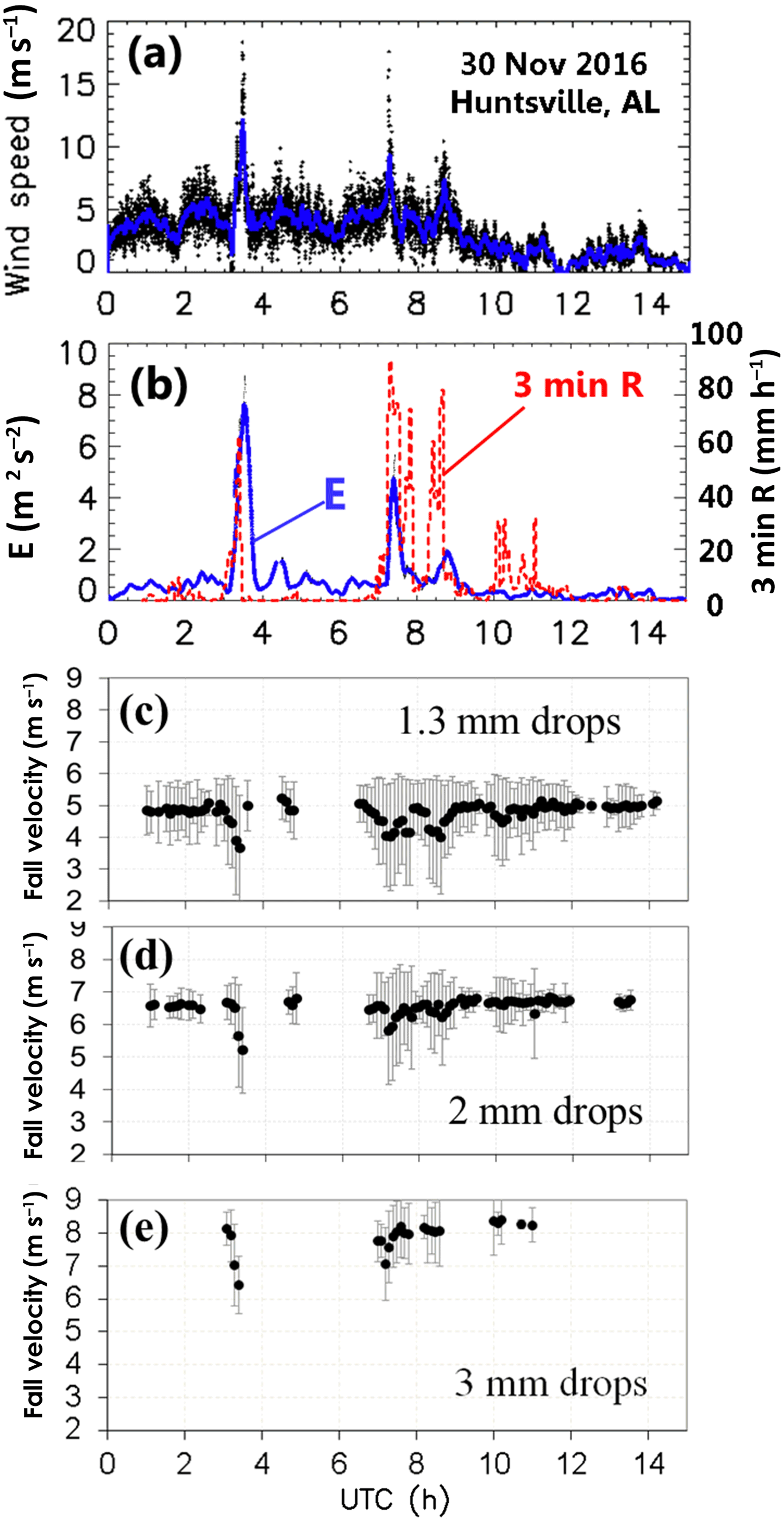
Figure 4(a) As in Fig. 2a except for 30 November 2016 event. (b) As in Fig. 2b. (c) Mean and ±1σ SD of fall speeds from 2DVD for 1.3±0.1 mm sizes. (d, e) As in (c) but for 2±0.1 and 3±0.1 mm sizes, respectively.
To expand on this observed correlation, Fig. 5 shows scatterplots of the mean fall speed and standard deviation vs. E for the 1.3 mm drops (panels a and b), while panels c and d and e and f show the same but for the 2 and 3 mm drops, respectively. The mean fall speed decreases with increasing E nearly linearly for E>1 m2 s−2 but less so for the 3 mm size drops (Stout et al., 1995). This decrease relative to Gunn–Kinzer terminal fall speeds is termed as “sub-terminal” and our data are in general agreement with Montero-Martinez and Garcia-Garcia (2016), who found an increase in the numbers of sub-terminal drops with sizes between 1 and 2 mm under windy conditions using a 2-D precipitation probe with resolution of 200 µm (similar to 2DVD) but without a wind fence. The standard deviation of fall speeds (σf) vs. E is shown in panels 5b, d and f. When E>1 m2 s−2, the σf is nearly constant at 1.5 m s−1 for both 1.3 and 2 mm drop sizes and constant at 1 m s−1 for the 3 mm size. For E<1, the σf is more variable and essentially uncorrelated with E. From the discussion related to Figs. 1b and c and 3b and c, σf values exceeding approximately 0.5 m s−1 can be attributed to physical, not instrumental or finite bin width effects (see also Table 1). Thus, the fall speed distributions are considerably broadened when E>1 m2 s−2 due to increasing turbulence levels which is again consistent with the findings of Montero-Martinez and Garcia-Garcia (2016) as well as those of Garett and Yuter (2014). The latter observations, however, were of graupel fall speeds in winter precipitation using a multiangle snowflake camera (Garrett et al., 2012).
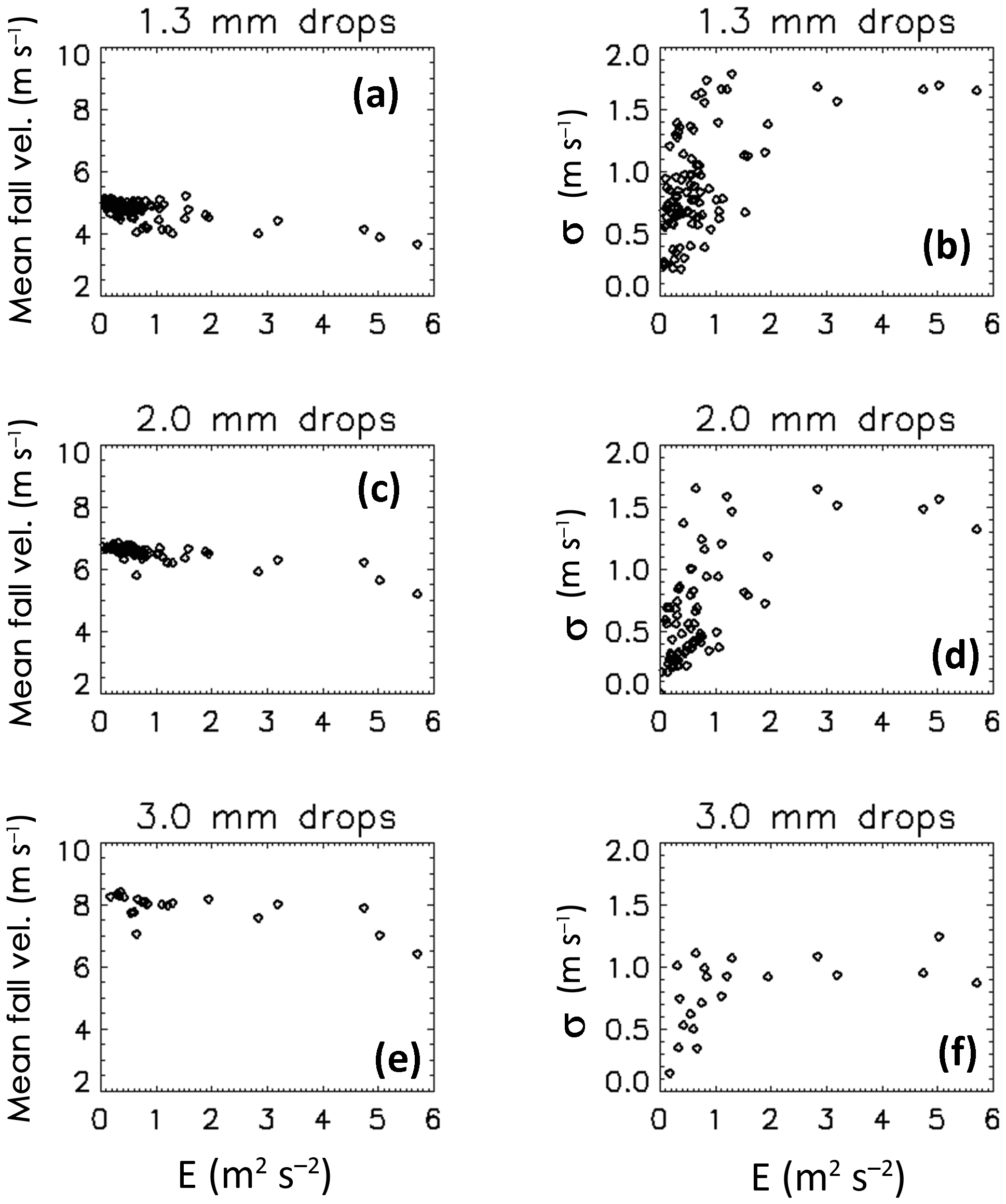
Figure 5(a, b) Mean fall speed and SD, respectively, vs. E for 1.3 mm sizes. (c, d) Same but for 2 mm sizes. (e, f) Same but for 3 mm.
We have reported on raindrop fall speed distributions using a high-resolution (50 µm) droplet spectrometer (MPS) collocated with moderate-resolution (170 µm) 2DVD (with both instruments inside a DFIR wind shield) to cover the entire size range (from 0.1 mm onwards) expected in natural rain. Turbulence intensity (E) was derived from wind/gust data at 10 m height following Garrett and Yuter (2014). For low turbulent intensities (E<0.4 m2 s−2), in the overlap region of the two instruments (0.7–2 mm), the mean fall speeds were in excellent agreement with each other for both the Greeley, CO, and Huntsville, AL, sites, giving high confidence in the quality of the measurements. For D<0.5 mm and down to 0.1 mm, the mean fall speeds from MPS from both sites were in remarkable agreement with FT fit to the laboratory data of Gunn and Kinzer (1949). In the overlap region, the mean fall speeds from the two instruments were in excellent agreement with the FT fit for the Huntsville site (no altitude adjustment required) and good agreement for the Greeley site (after adjustment for altitude of 1.4 km). For D>2 mm, the mean fall speeds from 2DVD were in excellent agreement with the FT fit at both sites.
Our histograms of fall speeds for 1 and 1.5 mm sizes under low turbulence intensity conditions (E<0.4 m2 s−2) from both MPS and 2DVD were in good agreement and did not show any evidence of either sub- or super-terminal speeds; instead, the histograms were symmetric with mean close to the Gunn–Kinzer terminal velocity with no significant broadening over that ascribed to instrument and/or finite bin width effects. (Note: sub-terminal implies fall speeds < 0.7 times the terminal fall speed whereas super-terminal implies >1.3 times terminal value; Montero-Martinez et al., 2009.) However, for the 0.5 and 0.7 mm sizes, from the histogram of fall speeds using the MPS under the same conditions occasional occurrences of both sub- and super-terminal fall speeds, after accounting for instrumental and finite bin width effects, cannot be ruled out.
The only comparable earlier study is by Montero-Martinez et al. (2009) who used collocated 2-D cloud and precipitation probes (2D-C, 2D-P) but restricted their data to calm wind conditions. Their main conclusion was that the distribution of the ratio of the measured fall speed to the terminal fall speed for 0.44 mm size, while having a mode at 1 m s−1 was strongly positively skewed with tails extending to 5 m s−1 especially at high rain rates. In our data for the 0.5 and 0.7 mm sizes shown in Figs. 1b and c and 3b and c, no such strong positive skewness was observed in the fall speed histograms, and the corresponding ratio of MPS-measured fall speeds to terminal values does not exceed 1.5 to 2.
Another study by Larsen et al. (2014) appears to confirm the ubiquitous existence of super-terminal fall speeds for sizes <1 mm using different instruments, one of which was a 2DVD similar to the one used in this study. However, it is well known that mismatched drops cause erroneous fall speed estimates from 2DVD for drops <0.5 mm (Schoenhuber et al., 2008; Appendix in Huang et al., 2010; Bernauer et al., 2015). It is not clear whether Larsen et al. (2014) accounted for this problem in their analysis. In addition, their 2DVD was not located within a DFIR-like wind shield.
In a later study using only the 2D-P probe, Montero-Martinez and Garcia-Garcia (2016) found sub-terminal fall speeds and broadened distributions under windy conditions for 1–2 mm sizes in general agreement with our results using the 2DVD. Stout et al. (1995) simulated the motion of drops subject to nonlinear drag in isotropic turbulence and determined that there would be a significant reduction of the average drop settling velocity (relative to terminal velocity) of greater that 35 % for drops around 2 mm size when the ratio of root mean square (rms) velocity fluctuations (due to turbulence) relative to drop terminal velocity is around 0.8. Whereas we did not have a direct measure of the rms velocity fluctuations, the proxy for turbulence intensity (E) related to wind gusts during supercell passage (very large E around 7 m2 s−2) and two squall-line passages (moderate E between 2 and 5 m2 s−2) clearly showed a significant reduction in mean fall speeds of 25–30 % relative to terminal speed for 1.3 and 2 mm sizes (and less so for 3 mm drops), with significant broadening of the fall speed distributions relative to calm conditions by nearly a factor of 1.5 to 2.
While our dataset is limited to three events they cover a wide range of rain rates, wind conditions and two different climatologies. One caveat is that the response of the DFIR wind shield to ambient winds in terms of producing subtle vertical air motions near the sensor area is yet to be evaluated as future work. Analysis of further events with direct measurement of turbulent intensity, for example using a 3-D sonic anemometer at the height of the sensor, would be needed to generalize our findings.
Data used in this paper can be accessed at ftp://lab.chill.colostate.edu/pub/kennedy/merhala/Bringi_et_al_2017_GRL_datasets/.
Viswanathan Bringi and Merhala Thurai declare they have no conflict of interest. Darrel Baumgardner is employed by Droplet Measurements Technologies, Inc. (Longmont, Colorado, USA), who manufacture the Meteorological Particle Spectrometer used in this study.
Two of the authors (Viswanathan N. Bringi and Merhala Thurai)
acknowledge support from the US National Science Foundation via
grant AGS-1431127. The assistance of Patrick Gatlin of NASA/MSFC is
gratefully acknowledged. Kevin Knupp and Carter Hulsey of the
University of Alabama in Huntsville processed the wind data.
Edited by: Gianfranco Vulpiani
Reviewed by: Hidde Leijnse and four anonymous referees
Atlas, D., Srivastava, R. C., and Sekhon, R. S.:. Doppler radar characteristics of precipitation at vertical incidence, Rev. Geophys., 11, 1–35, https://doi.org/10.1029/RG011i001p00001, 1973.
Barthazy, E., Göke, S., Schefold, R., and Högl, D.: An optical array instrument for shape and fall velocity measurements of hydrometeors, J. Atmos. Ocean. Tech., 21, 1400–1416, https://doi.org/10.1175/1520-0426(2004)021<1400:AOAIFS>2.0.CO;2, 2004.
Baumgardner, D., Abel, S., Axisa, D., Cotton, R., Crosier, J., Field, P., Gurganus, C., Heymsfield, A., Korolev, A., Krämer, M., Lawson, P., McFarquhar, G., Ulanowski, J. Z., and Shik Um, J.: Chapter 9: Cloud Ice Properties – In Situ Measurement Challenges, in: AMS Monograph on Ice Formation and Evolution in Clouds and Precipitation: Measurement and Modeling Challenges, edited by: Baumgardner, D., McFarquhar, G., and Heymsfield, A., American Meteorological Society, Boston, MA, 2016.
Beard, K. V.: Terminal velocity and shape of cloud and precipitation drops aloft, J. Atmos. Sci., 33, 851–864, https://doi.org/10.1175/1520-0469(1976)033<0851:TVASOC>2.0.CO;2, 1976.
Beard, K. V. and Pruppacher, H. R.: A determination of the terminal velocity and drag of small water drops by means of a wind tunnel, J. Atmos. Sci., 26, 1066–1072, https://doi.org/10.1175/1520-0469(1969)026<1066:ADOTTV>2.0.CO;2, 1969.
Belda, M., Holtanová, E., Halenka, T., and Kalvová, J.: Climate classification revisited: from Köppen to Trewartha, Clim. Res., 59, 1–13, https://doi.org/10.3354/cr01204, 2014.
Bernauer, F., Hürkamp, K., Rühm, W., and Tschiersch, J.: On the consistency of 2-D video disdrometers in measuring microphysical parameters of solid precipitation, Atmos. Meas. Tech., 8, 3251–3261, https://doi.org/10.5194/amt-8-3251-2015, 2015.
Foote, G. B. and Du Toit, P. S.: Terminal velocity of raindrops aloft, J. Appl. Meteorol., 8, 249–253, https://doi.org/10.1175/1520-0450(1969)008<0249:TVORA>2.0.CO;2, 1969.
Garrett, T. J. and Yuter, S. E.: Observed influence of riming, temperature, and turbulence on the fallspeed of solid precipitation, Geophys. Res. Lett., 41, 6515–6522, https://doi.org/10.1002/2014GL061016, 2014.
Garrett, T. J., Fallgatter, C., Shkurko, K., and Howlett, D.: Fall speed measurement and high-resolution multi-angle photography of hydrometeors in free fall, Atmos. Meas. Tech., 5, 2625–2633, https://doi.org/10.5194/amt-5-2625-2012, 2012.
Gunn, R. and Kinzer, G. D.: The terminal velocity of fall for water droplets in stagnant air, J. Meteorol., 6, 243–248, https://doi.org/10.1175/1520-0469(1949)006<0243:TTVOFF>2.0.CO;2, 1949.
Huang, G., Bringi, V. N., and Thurai, M.: Orientation angle distributions of drops after an 80 m fall using a 2-D video disdrometer, J. Atmos. Ocean. Tech., 25, 1717–1723, https://doi.org/10.1175/2008JTECHA1075.1, 2008.
Huang, G., Bringi, V. N., Cifelli, R., Hudak, D., and Petersen, W. A.: A methodology to derive radar reflectivity–liquid equivalent snow rate relations using c-band radar and a 2-D video disdrometer, J. Atmos. Ocean. Tech., 27, 637–651, https://doi.org/10.1175/2009JTECHA1284.1, 2010.
Knollenberg, R.: The optical array: an alternative to scattering or extinction for airborne particle size determination, J. Appl. Meteorol., 9, 86–103, https://doi.org/10.1175/1520-0450(1970)009<0086:TOAAAT>2.0.CO;2, 1970.
Knollenberg, R.: Three new instruments for cloud physics measurements: the 2–D spectrometer probe, the forward scattering spectrometer probe and the active scattering aerosol spectrometer, in: International Conference on Cloud Physics, 26–30 July 1976, Boulder, CO, USA, American Meteorological Society, 554–561, 1976.
Knollenberg, R.: Techniques for probing cloud microstructure, in: Clouds, Their Formation, Optical Properties and Effects, edited by: Hobbs, P. V. and Deepak, A., Academic Press, New York, USA, 495 pp., 1981.
Korolev, A. V.: Reconstruction of the sizes of spherical particles from their shadow images. Part I: Theoretical considerations, J. Atmos. Ocean. Tech., 24, 376–389, https://doi.org/10.1175/JTECH1980.1, 2007.
Korolev, A. V., Kuznetsov, S. V., Makarov, Y. E., and Novikov, V. S.: Evaluation of measurements of particle size and sample area from optical array probes, J. Atmos. Ocean. Tech., 8, 514–522, https://doi.org/10.1175/1520-0426(1991)008<0514:EOMOPS>2.0.CO;2, 1991.
Korolev, A. V., Strapp, J. W., and Isaac, G. A.: Evaluation of the accuracy of PMS optical array probes, J. Atmos. Ocean. Tech., 15, 708–720, https://doi.org/10.1175/1520-0426(1998)015<0708:EOTAOP>2.0.CO;2, 1998.
Larsen, M. L., Kostinski, A. B., and Jameson, A. R.: Further evidence for super terminal drops, Geophys. Res. Lett., 41, 6914–6918, https://doi.org/10.1002/2014GL061397, 2014.
List, R., Donaldson, N. R., and Stewart, R. E.: Temporal evolution of drop spectra to collisional equilibrium in steady and pulsating rain, J. Atmos. Sci., 44, 362–372, https://doi.org/10.1175/1520-0469(1987)044<0362:TEODST>2.0.CO;2, 1987.
Löffler-Mang, M. and Joss, J.: An optical disdrometer for measuring size and velocity of hydrometeors, J. Atmos. Ocean. Tech., 17, 130–139, https://doi.org/10.1175/1520-0426(2000)017<0130:AODFMS>2.0.CO;2, 2000.
Montero-Martinez, G. and Garcia-Garcia, F.: On the behavior of raindrop fall speed due to wind, Q. J. Roy. Meteor. Soc., 142, 2794, https://doi.org/10.1002/qj.2794, 2016.
Montero-Martinez, G., Kostinski, A. B., Shaw, R. A., and Garcia-Garcia, F.: Do all raindrops fall at terminal speed?, Geophys. Res. Lett., 36, L11818, https://doi.org/10.1029/2008GL037111, 2009.
Notaroš, B., Bringi, V. N., Kleinkort, C., Kennedy, P., Huang, G.-J., Thurai, M., Newman, A. J., Bang, W., and Lee, G.: Accurate characterization of winter precipitation using multi-angle snowflake camera, visual hull, advanced scattering methods and polarimetric radar, Atmosphere, 7, 81–111, https://doi.org/10.3390/atmos7060081, 2016.
Rasmussen, R., Baker, B., Kochendorfer, J., Meyers, T., Landolt, S., Fischer, A. P., Black, J., Thériault, J. M., Kucera, P., Gochis, D., Smith, C., Nitu, R., Hall, M., Ikeda, K., and Gutmann, E.: How well are we measuring snow: the NOAA/FAA/NCAR winter precipitation test bed, B. Am. Meteorol. Soc., 93, 811–829, https://doi.org/10.1175/BAMS-D-11-00052.1, 2012.
Rosewell, C. J.: Rainfall kinetic energy in Eastern Australia, J. Clim. Appl. Meteorol., 25, 1695–1701, https://doi.org/10.1175/1520-0450(1986)025<1695:RKEIEA>2.0.CO;2, 1986.
Schönhuber, M., Lammer, G., and Randeu, W. L.: One decade of imaging precipitation measurement by 2D-video-distrometer, Adv. Geosci., 10, 85–90, https://doi.org/10.5194/adgeo-10-85-2007, 2007.
Schönhuber, M., Lammar, G., and Randeu, W. L.: The 2-D-video-distrometer, in: Precipitation: Advances in Measurement, Estimation and Prediction, edited by: Michaelides, S. C., Springer, Berlin, Heidelberg, Germany, 3–31, 2008.
Sekhon, R. S. and Srivastava, R. C.: Doppler radar observations of drop-size distributions in a thunderstorm, J. Atmos. Sci., 28, 983–994, https://doi.org/10.1175/1520-0469(1971)028<0983:DROODS>2.0.CO;2, 1971.
Stout, J. E., Arya, S. P., and Genikhovich, E. L.: The effect of nonlinear drag on the motion and settling velocity of heavy particles, J. Atmos. Sci., 52, 3836–3848, https://doi.org/10.1175/1520-0469(1995)052<3836:TEONDO>2.0.CO;2, 1995.
Testik, F. Y. and Rahman, M. K.: High-speed optical disdrometer for rainfall microphysical observations, J. Atmos. Ocean. Tech., 33, 231–243, https://doi.org/10.1175/JTECH-D-15-0098.1, 2016.
Thériault, J. M., Rasmussen, R., Petro, E., Trépanier, J., Colli, M., and Lanza, L. G.: Impact of Wind Direction, Wind Speed, and Particle Characteristics on the Collection Efficiency of the Double Fence Intercomparison Reference, J. Appl. Meteorol. Clim., 54, 1918–1930, https://doi.org/10.1175/JAMC-D-15-0034.1, 2015.
Thurai, M., Huang, G.-J., Bringi, V. N., Randeu, W. L., and Schönhuber, M.: Drop Shapes, Model Comparisons, and Calculations of Polarimetric Radar Parameters in Rain, J. Atmos. Ocean. Tech., 24, 1019–1032, https://doi.org/10.1175/JTECH2051.1, 2007.
Thurai, M., Bringi, V. N., Szakáll, M., Mitra, S. K., Beard, K. V., and Borrmann, S.: Drop shapes and axis ratio distributions: comparison between 2-D video disdrometer and wind-tunnel measurements, J. Atmos. Ocean. Tech., 26, 1427–1432, https://doi.org/10.1175/2009TECHA1244.1, 2009.
Thurai, M., Bringi, V. N., Petersen, W. A., and Gatlin, P. N.: Drop shapes and fall speeds in rain: two contrasting examples, J. Appl. Meteorol. Clim., 52, 2567–2581, https://doi.org/10.1175/JAMC-D-12-085.1, 2013.
Thurai, M., Gatlin, P., Bringi, V. N., Petersen, W., Kennedy, P., Notaroš, B., and Carey, L.: Toward completing the raindrops size spectrum: case studies involving 2-D-video disdrometer, droplet spectrometer, and polarimetric radar measurements, J. Appl. Meteorol. Clim., 56, 877–896, https://doi.org/10.1175/JAMC-D-16-0304.1, 2017.
Trewartha, G. T. and Horn, L. H.: Introduction to Climate, 5th ed,. McGraw Hill, New York, USA, 416 pp., 1980.
Yu, C.-K., Hsieh, P.-R., Yuter, S. E., Cheng, L.-W., Tsai, C.-L., Lin, C.-Y., and Chen, Y.: Measuring droplet fall speed with a high-speed camera: indoor accuracy and potential outdoor applications, Atmos. Meas. Tech., 9, 1755–1766, https://doi.org/10.5194/amt-9-1755-2016, 2016.