2.1 Site description

Measurements were made at the SMEAR II station, a boreal coniferous forest in Hyytiälä in southern Finland ($\mathrm{61}{}^{\circ }{\mathrm{51}}^{\prime }$ N, $\mathrm{24}{}^{\circ }{\mathrm{17}}^{\prime }$ E; 181 m a.s.l.) during the years from 2013 to 2017. The site is dominated by Scots pine (Pinus sylvestris L.) with some Norway spruce (Picea abies (L.) Karst.) and deciduous trees (e.g., Betula sp., Populus tremula, and Sorbus aucuparia) within at least a 150 m radius from the measurement mast. The tree density is $\sim \mathrm{1170}{\mathrm{ha}}^{-\mathrm{1}}$ (Ilvesniemi et al., 2009), and the canopy height increased from approximately 18 to 20 m during the measurement years. The Scots pine stand was established in 1962 (Hari and Kulmala, 2005). The long-term annual mean precipitation and the annual mean temperature are 711 mm and 3.5 ^∘C, respectively (Pirinen et al., 2012).

2.2 Eddy covariance measurements and flux processing

EC measurements were made at a height of 23 m using an ultrasonic anemometer (Solent Research HS1199, Gill Instruments, Lymington, UK) to measure three wind components at a 10 Hz frequency and an Aerodyne quantum cascade laser spectrometer (QCLS, Aerodyne Research, Billerica, MA, USA) that measured COS, CO₂, water vapor (H₂O), and (beginning in 2015) carbon monoxide (CO) mole fractions (also at 10 Hz). The gas flow rate was approximately 10 slpm (standard liters per minute). Background measurements of high-purity nitrogen were made every 30 min for 26 s to remove background spectral structures (Kooijmans et al., 2016). EC data were processed using the EddyUH software (Mammarella et al., 2016) following the recommendations given in Kohonen et al. (2020). Raw data were despiked based on the maximum difference allowed between two subsequent data points, two-dimensional coordinate rotation was used to rotate the coordinate frame, and turbulent fluctuations were determined from linear detrending. Lag times of COS, carbon monoxide (CO), and carbon dioxide (CO₂) were determined from the maximum cross-covariance of CO₂ with vertical wind speed (w), while the lag time of water vapor (H₂O) was determined from the maximum cross-covariance of H₂O with w. High-frequency spectral corrections were calculated according to Mammarella et al. (2009), so that the response time of CO₂ was also used for COS and CO spectral corrections. Low-frequency correction was done according to Rannik and Vesala (1999).

Quality screening was applied to the data by tests for flux stationarity (≤0.3) and limits for kurtosis ($\mathrm{1}<\text{Ku}<\mathrm{8}$) and skewness ($-\mathrm{2}<\text{Sk}<\mathrm{2}$). In addition, only 100 spikes were allowed for each 30 min period, and the second wind rotation angle was not allowed to exceed 10^∘. Friction velocity (u_∗) filtering with a threshold of 0.3 m s⁻¹ was applied to exclude time periods with low turbulence. Finally, fluxes were gap filled using the function

where I is the photosynthetic photon flux density; D is the vapor pressure deficit (VPD); and a, b, c, and d are fitting parameters (Kohonen et al., 2020).

The uncertainty of the cumulative flux was estimated using a bootstrap method. This was done because the uncertainty of single 30 min fluxes consists of both random and systematic uncertainties as well as the uncertainty of the gap-filling function that cannot be mixed with flux measurement uncertainties. In the bootstrap method, we assumed a 20 % total uncertainty that mostly consists of processing uncertainty (Kohonen et al., 2020), and a synthetic data set was randomly sampled from the data set (including the 20 % uncertainty) 10 000 times. The synthetic data sets consisted of an amount of data points equal to those in the original data set; however, as the samples were drawn at random, some data points may be included several times, whereas other points may not be included at all. The overall uncertainty was calculated as the difference to the 95th percentile of the 10 000 bootstrap sample sums. The FCOS record comprises 32 months over 5 years, of which 51 % is gap filled, representing 23 152 measured 30 min fluxes, which provides the opportunity to observe and analyze the interannual variability.

2.3 Environmental variables and the commencement of the carbonyl sulfide uptake period

T_a and relative humidity (RH) were measured at heights of 16.8 and 33.6 m, and an average of the two heights was assumed to best represent T_a and RH at a height of 23 m, where the EC measurements were made. T_a was measured using Pt100 sensors, and RH was calculated from the H₂O mole fraction measured with a LI-COR LI-840 infrared light absorption analyzer and a Pt100 sensor. Photosynthetically active radiation (PAR) from 400 to 700 nm was measured above the canopy using a LI-COR LI-190SZ quantum sensor. Soil temperature (T_s) in the A horizon (2–5 cm in the mineral soil) was determined as the mean of five locations representative of the forest floor, with data measured using Philips KTY81-110 temperature sensors. Volumetric soil water content (SWC) in the A horizon (2–6 cm depth) was also calculated as the mean of five different locations, with data measured using a Campbell TDR100 time-domain reflectometer. The optical LAI was calculated from continuous measurements of PAR with eight sensors at a height of 0.6 m near the flux tower and one sensor above the forest using the inverse Beer–Lambert equation parameterized separately for direct beam and diffuse radiation. The wintertime LAI (October–March) was interpolated. The vapor pressure deficit (VPD) was calculated as the difference between the saturation water vapor pressure (e_s) and the actual water vapor pressure (e_a) as follows:

where

Here, T_a is air temperature, and RH is the relative humidity of air, which are both calculated as an average of measurements done at heights of 16.8 and 33.6 m, representing the flux measurement height of 23 m.

The commencement of the growing season was determined, following the recommendations of Suni et al. (2003a), by a moving average T_a with a 5 d window (with a threshold of 3.3 ^∘C indicating the start of photosynthetic uptake) and by a T_a-dependent variable S that describes the stage of physiological development, introduced by Pelkonen and Hari (1980):

where

In Eq. (6), a=2 and c=600 are fitted constants, as in Suni et al. (2003a) and Pelkonen and Hari (1980), and Eqs. (5) and (6) were solved with the Euler method with a 30 min time step dt. For simplicity, we scaled S by c as in Suni et al. (2003a). The threshold for the start of the growing season by this method was $S/c>\mathrm{1.81}$, as in Suni et al. (2003a), and S at i=0 was defined as S₀=0. The S parameter has previously been used in ecosystem research, especially to determine the spring recovery (Suni et al., 2003a; Pelkonen and Hari 1980) and biosphere modeling in JSBACH (Mäkelä et al., 2016, 2019). This is especially useful at high latitudes due to varying spring conditions. When temperatures may change by over 10 ^∘C in 1 d and vary both below and above 0 ^∘C, the more traditional heat sum is not a good approximation for phenology. The S parameter takes the temperature history and subzero temperatures into account, which the traditional heat sum does not.

Although the progress of COS uptake in the spring is a gradual process, we get a better insight into its evolution and its yearly variations if we define a threshold for the onset of COS uptake. For the commencement of the significant COS uptake period, we used the date when the midday FCOS permanently (for at least 5 consecutive days) fell below 30 % of the median of the minimum FCOS from all years (maximum uptake) (see Table S1 in the Supplement). Daytime was defined as periods when the solar elevation angle was greater than zero.

2.4 Multivariate linear regression analysis

Multivariate linear regression analysis was used to find the dependencies of the FCOS on various environmental factors: VPD, T_a, PAR, RH, T_s, SWC, net radiation (R_n), and the atmospheric COS mixing ratio. All of the computations were done in R (R Core Team, 2019) using “Base” functions, and the variance inflation factor (VIF) was computed using the “vif” function within the “car” package (Fox and Weisberg, 2011). Only measured (non-gap-filled) FCOS data were used for the analysis so that at least 50 % of data had to exist to calculate, e.g., daily averages.

We used the VPD and T_a within the same linear regression model, despite knowing that the VPD is obtained using T_a. However, the VPD is computed as an exponential function of T_a, which technically does not break the assumption of linear independence of explanatory variables within the regression model. Nonetheless, there is naturally some multicollinearity among almost all environmental factors, which must be treated. The VIF was used to see whether the multicollinearity among explanatory variables within each regression model was of an acceptable level so as not to brake the assumption of the linear regression analysis. The VIF quantifies the severity of multicollinearity in an ordinary least squares regression analysis. It provides an index that measures how much the variance (the square of the estimate's standard deviation) of an estimated regression coefficient is increased because of collinearity. VIF<10 is a commonly used cutoff for acceptable multicollinearity. All of the models that included more than one variable were tested with the VIF, which was less than 10 in all cases. Two variables showing the same physical quantity were never used in the same model (T_a and T_s, PAR and R_n, or RH and VPD).

2.5 Wavelet coherence analysis

Magnitude-squared wavelet coherence was computed using the “wcoherence” function, which uses the analytic Morlet wavelet (Grinsted et al., 2004; Lau and Weng, 1995), in MATLAB (MATLAB R2019a). As input to the function, fluxes were first quality screened and gap filled. For longer measurement gaps (e.g., winter), fluxes were forced to zero. Thus, the wavelet coherence is also zero for longer data gaps. Environmental variables (PAR, T_a, and VPD) were averaged from 1 to 30 min values to match the time stamp of the flux data.

2.6 Parameterization of carbonyl sulfide fluxes

The FCOS were parameterized using the PAR, T_a, VPD, and total LAI data over the 32 months on a daily scale. As the ecosystem COS uptake is dominated by the canopy uptake (70 % at minimum according to Sun et al., 2018) and is process-wise very close to the CO₂ uptake, we formulated the parameterization as follows:

Here,

In the above expressions, a, b, c, d, and e are fitting parameters, and four functions are simplified from the corresponding dependencies of the CO₂ uptake on PAR and T_a (with S being a function of T_a; see Sect. 2.3) (according to Mäkelä et al., 2008), VPD (Dewar et al., 2018), and LAI (Peltoniemi et al., 2015). Parameters $a=-\mathrm{341.81}$, b=1000, $c=-\mathrm{0.77}$, and d=1.03 were optimized using the “fminsearchbnd” function in MATLAB to find the smallest root-mean-square error of the parameterized FCOS against the measured (non-gap-filled) FCOS. The fminsearchbnd function finds the minimum of a constrained multivariable function using a derivative-free method (D'Errico, 2021). Parameters were given upper and lower limits of $a\in [\mathrm{5},\mathrm{500}]$, $b\in [\mathrm{10},\mathrm{1000}]$, $c\in [-\mathrm{3},\mathrm{3}]$, and $d\in [\mathrm{1},\mathrm{5}]$. It is to be noted that parameter b is at its upper limit. However, increasing the limit (until infinity) for parameter b only resulted in a higher value for parameter a, without significantly improving the overall fit. Parameter e=0.18 was fixed before optimizing the other parameters according to a previous study by Peltoniemi et al. (2015), as parameter e is related to ecosystem phenology specific to the site and is believed not to be gas dependent. Although recognizing that other more complex formulas with more fitting parameters could provide better correspondence with observations, we desired to keep the parameterization simple for the sake of generic process description: here, FPAR describes the stomatal response to PAR and includes all other light-dependent processes, FS is the phenology of biochemical reactions, FVPD is the stomatal regulation, and FLAI is the amount of foliage and canopy light penetration. The VPD response was based on Dewar et al. (2018), who showed that the FVPD function is predicted theoretically by a variety of stomatal optimization models and explains observed stomatal responses better than the empirical Ball–Berry model (Ball et al., 1987).

2.7 Boreal region carbonyl sulfide fluxes

We scaled up the FCOS parameterization to the whole boreal region to evaluate FCOS simulations by SiB4. SiB4 (Haynes et al., 2019) is a continuation of the SiB3 model in which COS exchange was implemented by Berry et al. (2013). One of the added capabilities of SiB4 that was not present in SiB3 is that it simulates fluxes of multiple plant functional types (PFTs) in a grid cell and allows the selection of fluxes from a single PFT. This is beneficial for the analysis in this study, as we want to undertake a comparison with observation-based data from evergreen needleleaf forests (ENFs).

The COS module of SiB4 was recently updated with the COS soil exchange model of Ogee et al. (2016), and the standard COS mole fraction of 500 ppt was replaced by COS mole fraction fields that vary in space and time, including seasonal and diurnal variability (Kooijmans et al., 2021). The meteorological data that drive SiB4 are from the Modern-Era Retrospective analysis for Research and Applications, Version 2 (MERRA2), available from 1980 onward (Gelaro et al., 2017). The simulations of SiB4 are preceded by a spin-up from 1850 to 1979 to initialize the carbon pools using the climatological average of available MERRA2 data (Smith et al., 2020). We ran SiB4 with 3-hourly output globally, and we selected grid cells (at $\mathrm{0.5}{}^{\circ }\times \mathrm{0.5}{}^{\circ }$ resolution) where ENFs cover more than 30 % of the land area in the Northern Hemisphere for the analysis. The information on areal coverage of different PFTs was retrieved from MODIS data (Lawrence and Chase, 2007). Finally, only the fluxes representing ENFs were selected.

To obtain COS biosphere fluxes for the whole boreal region based on the FCOS observations in Hyytiälä, we calibrated the SiB4 PAR, LAI, VPD, and T_a for the grid cell where Hyytiälä is located against observations. The obtained calibration is shown in Fig. S10 in the Supplement. The in situ LAI is the all-sided leaf area index, whereas the SiB4 LAI is projected leaf area index, which explains the large difference between the two LAI data. We then applied the parameterization represented in Eqs. (7)–(11) to the whole boreal region (based on the ENF grid cell selection described in the previous paragraph) using the SiB4 meteorological and phenological data.

3.1 Environmental conditions

The PAR ranged from 0 to 1900 $\mathrm{\mu }\mathrm{mol}{\mathrm{m}}^{-\mathrm{2}}{\mathrm{s}}^{-\mathrm{1}}$, with the highest amount of radiation usually reached in June (Fig. 1). May 2017 and July 2014 had higher monthly median PAR values (285 and 303 $\mathrm{\mu }\mathrm{mol}{\mathrm{m}}^{-\mathrm{2}}{\mathrm{s}}^{-\mathrm{1}}$, respectively) than other years (Fig. S1). T_a varied from a minimum of −28 ^∘C in January 2016 to a maximum of 29 ^∘C in July 2014, while the mean T_a of the whole measurement period was 4.9 ^∘C. The highest monthly median T_a was reached in July 2014 (19.5 ^∘C). May–June 2013 and July 2014 were warmer compared with other years, whereas April 2017 was colder than usual (monthly median T_a of 0.4 ^∘C). T_s had more moderate variation from 2.7 to 17.5 ^∘C, with an average over the whole period of 5.8 ^∘C. The VPD ranged from 0 to 2.7 kPa, and the highest VPD was reached during May–July, depending on the year. May 2013 and 2016 were dryer than usual with a monthly average VPD of 0.6 kPa. July 2014 and August 2015 were also unusually dry with a monthly median VPD of 0.7 and 0.5 kPa, respectively, but these months were not considered to be drought because the SWC remained at a normal level (well above 0.1 m³ m⁻³). The SWC did not vary much between different years during the growing seasons (April–October), but August 2015 and 2016 had a higher SWC than other years. The minimum SWC (0.1 m³ m⁻³) was usually reached in August–September, whereas it was highest right after snowmelt in April (monthly median 0.3 m³ m⁻³). The LAI varied seasonally between 5 and 7 m² m⁻² with the maximum LAI reached in August in all years.

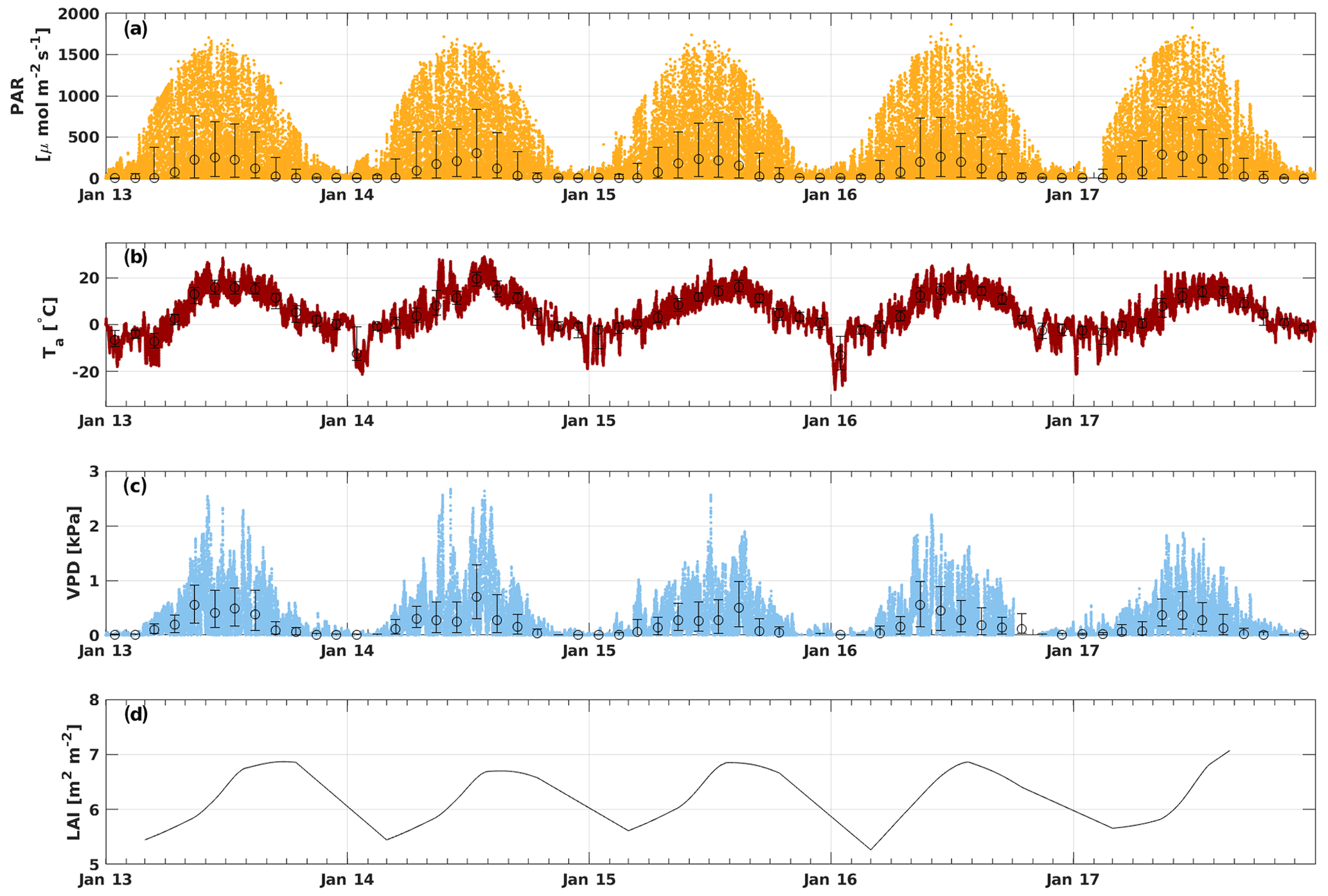
Figure 1Time series of PAR (a), T_a (b), VPD (c), and all-sided LAI (d). The small solid dots in panels (a)–(c) represent 30 min values, the larger open circles represent the monthly medians, and error bars show their 25th and 75th percentiles. The LAI is shown as daily smoothed values.

Download

3.2 Seasonality of the FCOS and their interannual variability

The FCOS (COS uptake indicated by a negative sign) showed a pronounced seasonal cycle (Figs. 2a–d, S2) with the most negative flux in summer (June–August); this was expected, as PAR, T_a, and T_s also had clear seasonal cycles (Figs. 1a–b, S3a).

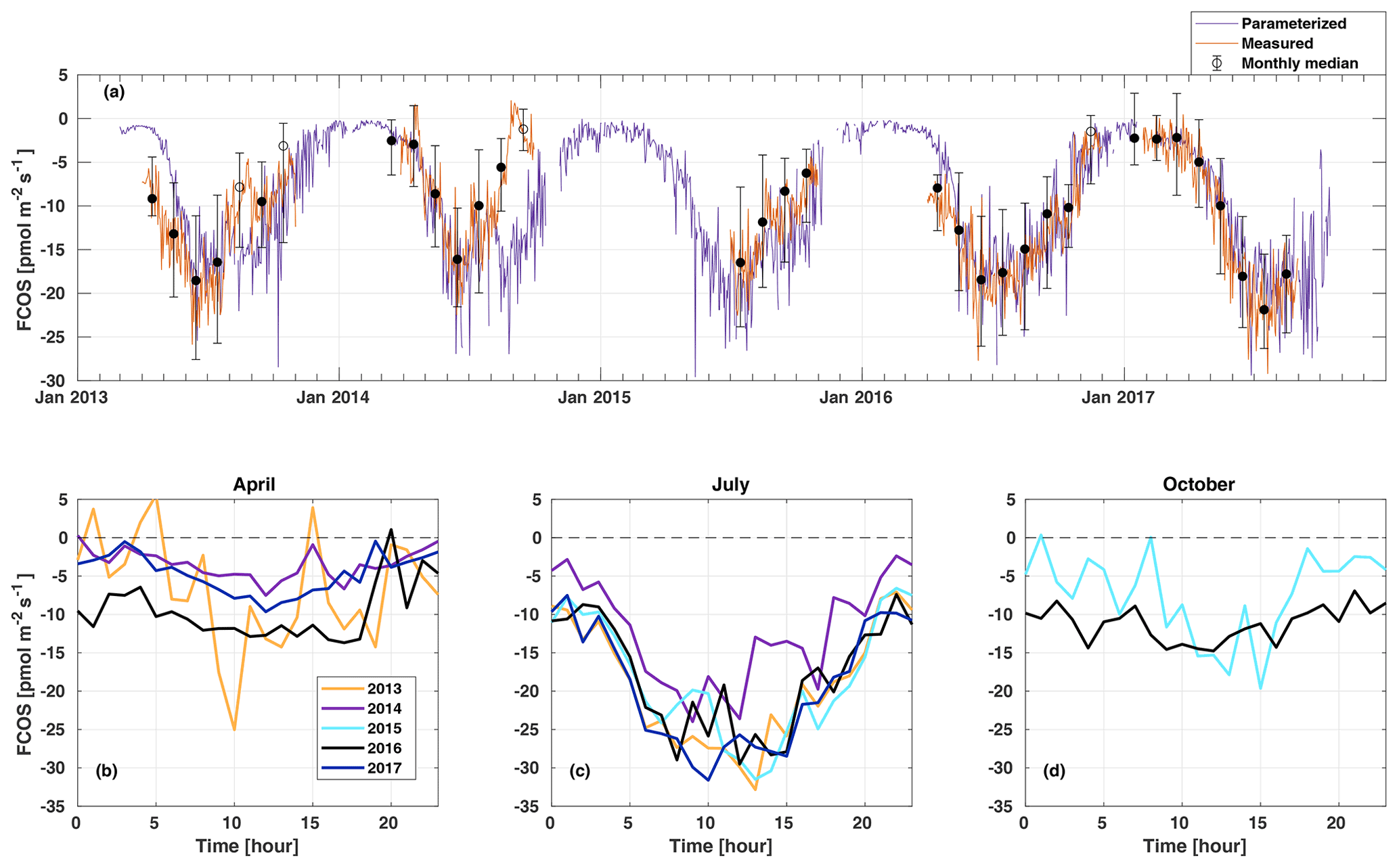
Figure 2Daily average net carbonyl sulfide flux (FCOS) time series (a) and median diurnal variation in FCOS in April (b), July (c), and October (d). A negative sign means COS uptake. Measured data (orange line in a) show daily gap-filled averages (see Sect. 2.2), and black circles represent the monthly medians. Filled circles mean that more than 20 % of data were measured, whereas empty circles indicate less than 20 % of measured data for that month. Whiskers show the 25th and 75th percentiles. The purple line in panel (a) is the parameterized daily FCOS (see Eq. 1). Panels (b)–(d) represent measured (non-gap-filled) data only. No data are available for 2015 in April and for 2013, 2014, and 2017 in October. Parameterized values are shown for 5 full years. Times represent UTC+2 (local winter time).

Download

In April, the years 2013 and 2016 represented higher uptake than the years 2014 and 2017 (Fig. 2b). The significant COS uptake started on 15 April in 2013, based on a 3 d midday flux moving average being persistently below 30 % of the summer minimum (ca. −10 $\mathrm{pmol}{\mathrm{m}}^{-\mathrm{2}}{\mathrm{s}}^{-\mathrm{1}}$) (Table S1), and before 1 April (before measurements started) in 2016. The corresponding date was 28 April in both 2014 and 2017. Suni et al. (2003a) and Sevanto et al. (2006) studied the same forest stand as that used in this study, and they found that the spring recovery of the CO₂ exchange is controlled by T_a to a large extent, whereas the soil water availability is not a limiting factor. Snowmelt has also been used as a good proxy indicator for the start of the carbon uptake (Pulliainen et al., 2017) in the boreal region. Suni et al. (2003a) defined the photosynthetically active period as the point when the CO₂ flux reached 20 % of the maximum summer CO₂ flux. They found that the days on which the daily average or a moving average T_a with a 5 d window exceeded 4.0 or 3.3 ^∘C, respectively, coincided accurately with the commencement day of the photosynthetically active period. We analyzed the dependence of CO₂ flux on T_a for the period of this study, and no similar corresponding relationship was found for CO₂ nor for FCOS. When the median T_a of May in 2014 and 2017 was low (below 8 ^∘C), the FCOS remained above −9 $\mathrm{pmol}{\mathrm{m}}^{-\mathrm{2}}{\mathrm{s}}^{-\mathrm{1}}$, whereas it was ca. −13 $\mathrm{pmol}{\mathrm{m}}^{-\mathrm{2}}{\mathrm{s}}^{-\mathrm{1}}$ in 2013 and 2016 when the median T_a was ca. 13 ^∘C (Table S2, Fig. S1). During spring (April–May), the higher VPD was positively correlated with the COS uptake, but this resulted from higher T_a, which was also positively correlated (see Fig. 3b, c). The heat sum (sum of daily average temperatures that are above 0 ^∘C) did not influence the commencement of significant COS uptake in the spring (Fig. S4).

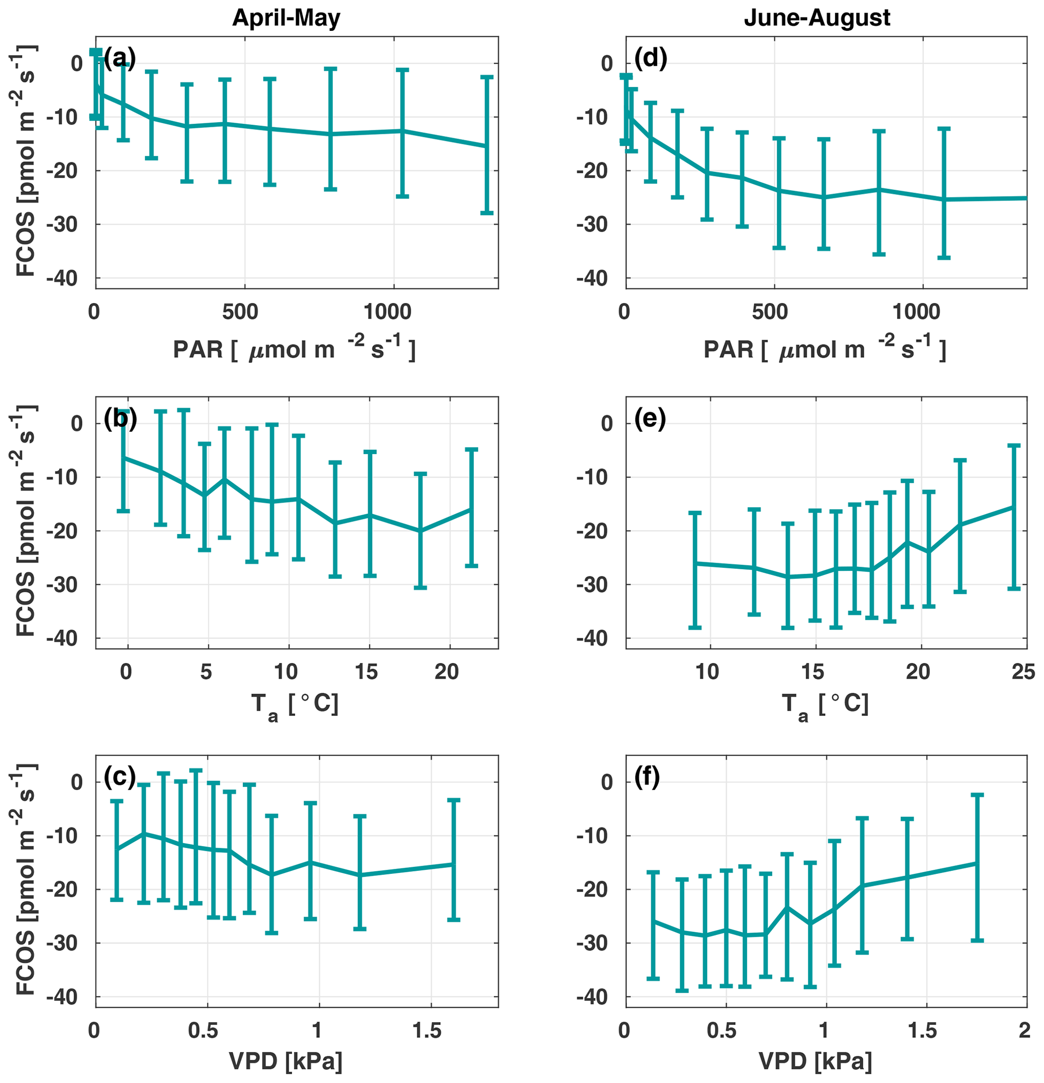
Figure 3The carbonyl sulfide flux (FCOS) relationship with environmental variables in spring (a–c) and summer (d–f). Panels (b), (c), (e), and (f) are filtered to high radiation only (photosynthetically active radiation, $\text{PAR}>\mathrm{500}\mathrm{\mu }\mathrm{mol}{\mathrm{m}}^{-\mathrm{2}}{\mathrm{s}}^{-\mathrm{1}}$). Data are binned in 12 equally sized bins, and whiskers represent the 25th and 75th percentiles. VPD represents the vapor pressure deficit.

Download

The COS uptake in July 2014 was at a significantly lower level in the afternoon than in other years (Fig. 2c). Moreover, the T_a and VPD maximum values in the afternoon were larger in July 2014 than in any other year (Fig. S1). This led to the most pronounced asymmetry in the uptake between the morning and afternoon in July 2014. The monthly median COS uptake was 54 % smaller in July 2014 compared with that in 2017 when the uptake was the highest (Table S2). The forest acted as a COS sink during nighttime throughout the measurement period (see Fig. 6). Previous measurements have found both nocturnal soil uptake (Sun et al., 2018) and uptake by foliage, as suggested by the stomatal conductance being nonzero throughout the night, indicating incomplete stomatal closure during nighttime (Kooijmans et al., 2017, 2019). Mosses and other cryptogams can also take up significant amounts of COS during the night when the soil is wet (Rastogi et al., 2018). Nighttime soil uptake in Hyytiälä was ca. −3 pmol m² s¹ (Sun et al., 2018), whereas the ecosystem-scale nighttime uptake in our study is ca. −10 pmol m² s¹. However, we did not measure the contribution from cryptogams. Thus, the nighttime COS uptake in Hyytiälä is likely a combination of soil and moss uptake but also has a larger contribution from the canopy (Kooijmans et al., 2017). The average nocturnal FCOS varied between −5 and −12 $\mathrm{pmol}{\mathrm{m}}^{-\mathrm{2}}{\mathrm{s}}^{-\mathrm{1}}$ throughout the year. Compared with July, the diurnal variation in FCOS was much smaller in April and October, especially in 2016 (Fig. 2b, c, d). The flux was close to zero but still indicated a small uptake during winter months when data were available in November 2016–March 2017 (monthly median between −2.4 and −1.5 $\mathrm{pmol}{\mathrm{m}}^{-\mathrm{2}}{\mathrm{s}}^{-\mathrm{1}}$) (Fig. 2a, Table S2). Suni et al. (2003b) found that light is the determining factor for the cessation of the growing season for the same stand. For the parameterized flux in Fig. 2a, see Sect. 3.4.

The lowest monthly median FCOS value (highest uptake) was −21.9 $\mathrm{pmol}{\mathrm{m}}^{-\mathrm{2}}{\mathrm{s}}^{-\mathrm{1}}$ in July 2017 (Table S2). In June 2014, the monthly FCOS value was −16.1 $\mathrm{pmol}{\mathrm{m}}^{-\mathrm{2}}{\mathrm{s}}^{-\mathrm{1}}$, which was the highest flux from the months with the largest uptake in each year. The lowest weekly FCOS value was −23.9 $\mathrm{pmol}{\mathrm{m}}^{-\mathrm{2}}{\mathrm{s}}^{-\mathrm{1}}$ in week 29 (20–26 July) in 2017, and the highest weekly FCOS value was −19.2 $\mathrm{pmol}{\mathrm{m}}^{-\mathrm{2}}{\mathrm{s}}^{-\mathrm{1}}$ in week 25 (16–22 July) in 2014 (from the weeks with the largest uptake in each year). Thus, the interannual variability in the maximum uptake was 26 % and 20 % in the monthly and weekly medians, respectively. The variability in the timing of the maximum weekly uptake was 6 weeks, occurring in week 23 in 2016 and week 29 in 2017 (Table S3).

3.3 Carbonyl sulfide flux relationship with light, air temperature, and vapor pressure deficit

Figure 3 presents the FCOS as a function of PAR, T_a, and VPD for April–May and June–August. Responses to the T_a and VPD were filtered to only include data with $\text{PAR}>\mathrm{500}\mathrm{\mu }\mathrm{mol}{\mathrm{m}}^{-\mathrm{2}}{\mathrm{s}}^{-\mathrm{1}}$ in order to avoid including a radiation-related correlation, as VPD and T_a are highly intercorrelated with PAR. For the responses without separation between spring and summer periods and without filtering for low PAR, see Fig. S5. The fluxes showed a clear relationship with PAR (Fig. 3a, d), even though the COS biochemical reactions and carbonic anhydrase (CA) activity are light independent and the FCOS respond to light mainly due to the light response of stomatal conductance (Kooijmans et al., 2019). Besides CA, carboxylating enzymes, ribulose-l,5-bisphosphate-carboxylase (RuBisCO) and phosphoenolpyruvate-carboxylase (PEP-Co), which are light dependent, contribute to COS metabolism (Protoschill-Krebs and Kesselmeier, 1992). However, it is not possible to separate these processes from EC flux measurements, and it has been shown that the main enzyme contributing to COS uptake in plants is CA (Protoschill-Krebs et al., 1996). Thus, we do not expect the role of PEP-Co and RuBisCO light dependency to exceed that of stomatal regulation. When T_a was high (Fig. 3e), in theory favoring uptake due to enhanced biochemical reactions in the mesophyll, the simultaneous occurrence of high VPD (Fig. 3f) limited uptake due to smaller stomatal conductance values (see Kooijmans et al., 2019). The fluxes tended to saturate as a function of T_a above 10 ^∘C in spring and increase (uptake decrease) above 15 ^∘C in summer (Fig. 3b and e, respectively). At 10 ^∘C in spring, the FCOS values were ca. −15 $\mathrm{pmol}{\mathrm{m}}^{-\mathrm{2}}{\mathrm{s}}^{-\mathrm{1}}$, whereas they were ca. −25 $\mathrm{pmol}{\mathrm{m}}^{-\mathrm{2}}{\mathrm{s}}^{-\mathrm{1}}$ in summer. These flux values correspond to a VPD of ca. 1 kPa in spring and summer, respectively. The nonzero value in the dark represents the ecosystem nocturnal COS uptake (Fig. 3a). The response curve saturated at high PAR values in the summer to approximately twice the level of those in spring. This saturation occurred above a PAR value of about 500 $\mathrm{\mu }\mathrm{mol}{\mathrm{m}}^{-\mathrm{2}}{\mathrm{s}}^{-\mathrm{1}}$. Correspondence with the VPD resembled that for T_a (Fig. 3c, f). The fluxes tended to increase (uptake decrease) when the VPD was above 0.8 kPa.

Table 1Results of the multivariate and univariate regression analysis for carbonyl sulfide (COS) flux at daily, weekly, and monthly timescales. The variables tested are the vapor pressure deficit (VPD), air temperature (T_a), photosynthetically active radiation (PAR), net radiation (R_n), soil water content (SWC), soil temperature (T_s), precipitation (Precip), relative humidity (RH), and the atmospheric COS mixing ratio (χ_COS). Two variables related to a similar physical quantity were never used in the same model (T_a and T_s, PAR and R_n, or RH and VPD). All of the models that included more than one variable were tested with the variation inflation factor, which was less than 5 in all cases, showing that the intercorrelation of the variables is negligible.

Download Print Version | Download XLSX

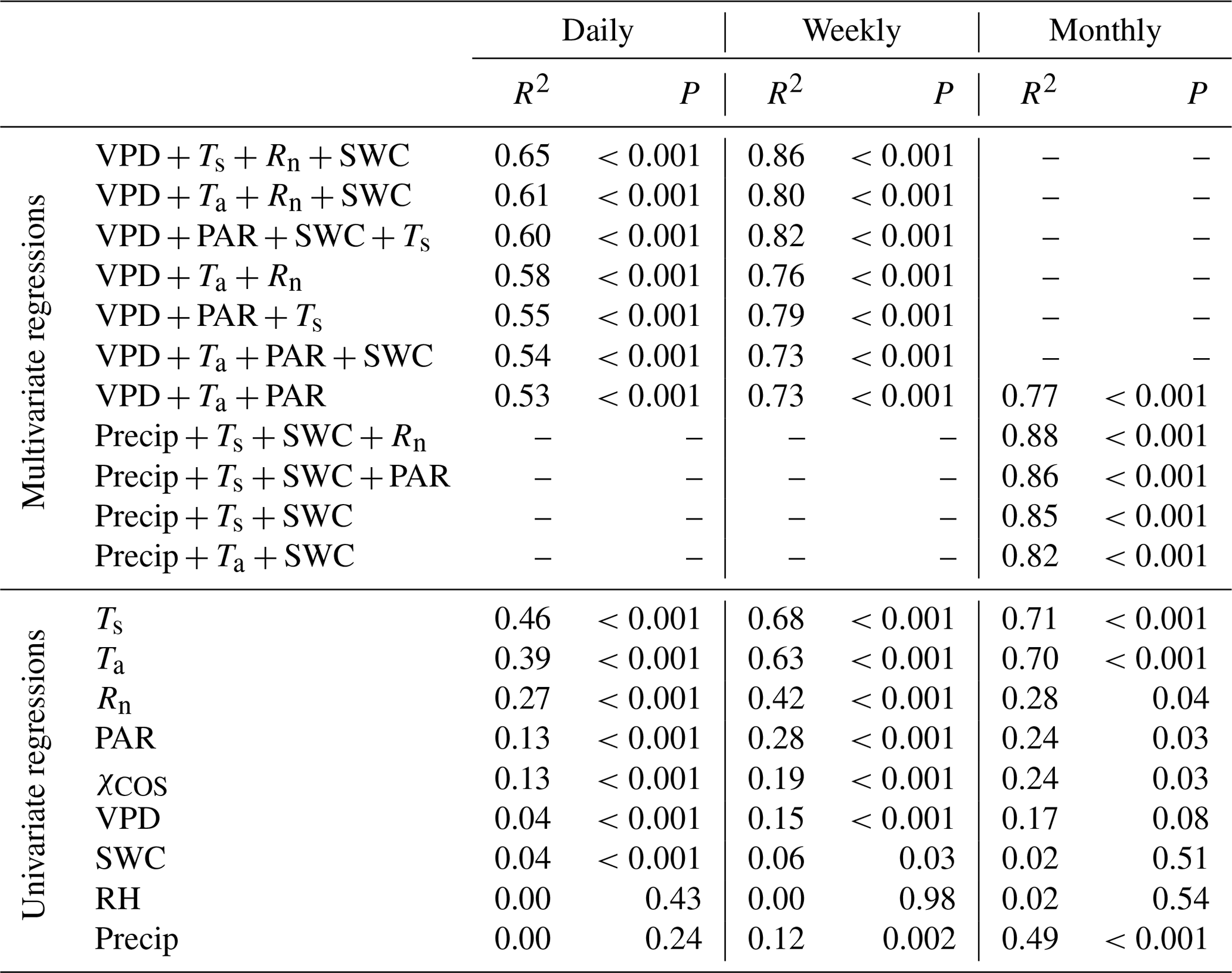
We analyzed the relationship between the FCOS and environmental factors using multivariate and univariate linear regressions combining the VPD, relative humidity (RH), net radiation (R_n) or PAR, T_a or T_s, SWC, and precipitation. Their intercorrelation was of an acceptable level for the analysis (Sect. 2.4). Daily FCOS were best explained by the VPD, R_n, T_s, and SWC (R²=0.65, Table 1), where the contribution of SWC was minor (see also Kooijmans et al., 2019). Primary variables directly interacting with the canopy (VPD, PAR, and T_a) explained FCOS with R²=0.53. On a monthly scale, replacing the VPD with precipitation gave the highest R² value (0.88), while R² (VPD, PAR, T_a)=0.77. Univariate analysis for single factors revealed that the temperature was the most important factor governing the FCOS (Table 1). Maignan et al. (2021) studied the importance of different drivers (PAR, T_a, VPD, LAI, and SWC) for stomatal conductance in Hyytiälä using random forest models. The three most important drivers for stomatal conductance were (in order) PAR, T_a, and VPD. This is well in line with our univariate analyses that ranked temperature and radiation as the most important drivers of the FCOS, which is mostly regulated by stomatal conductance. The importance of the VPD is larger on longer timescales. While some of the interactions are nonlinear, as seen from Fig. 3 and Eqs. (8)–(11), the linear regression analysis still provides information on the relative importance of the environmental variables, as nonlinear correlations usually have a high linear correlation as well.

We also applied wavelet analysis (Torrence and Gilbert, 1998). This revealed coherence between the FCOS and PAR on daily and yearly temporal scales without any significant time lags between them (Fig. S6), indicating a rapid response of stomata to PAR. The pattern of the coherence between the FCOS and VPD was very similar, although the coherence values were somewhat smaller than those with PAR. The coherence between T_a and the FCOS had a 3 h lag on a daily scale, so the FCOS minimum (the uptake maximum) was reached before the T_a maximum. T_a usually reached its daily maximum in the afternoon between 15:00 and 17:00 (not shown; all times are given in UTC+2, local winter time, throughout the paper), whereas the FCOS minima were most frequently between 10:00 and 14:00 (Fig. 2c). This is caused by the VPD and PAR, which control the stomatal conductance (Fig. S6; Kooijmans et al., 2019). In addition, Maignan et al. (2021) showed that the internal conductance is driven by T_a and limits the total conductance, especially in the afternoon. On a yearly scale, there was no significant phase difference between T_a and the FCOS.

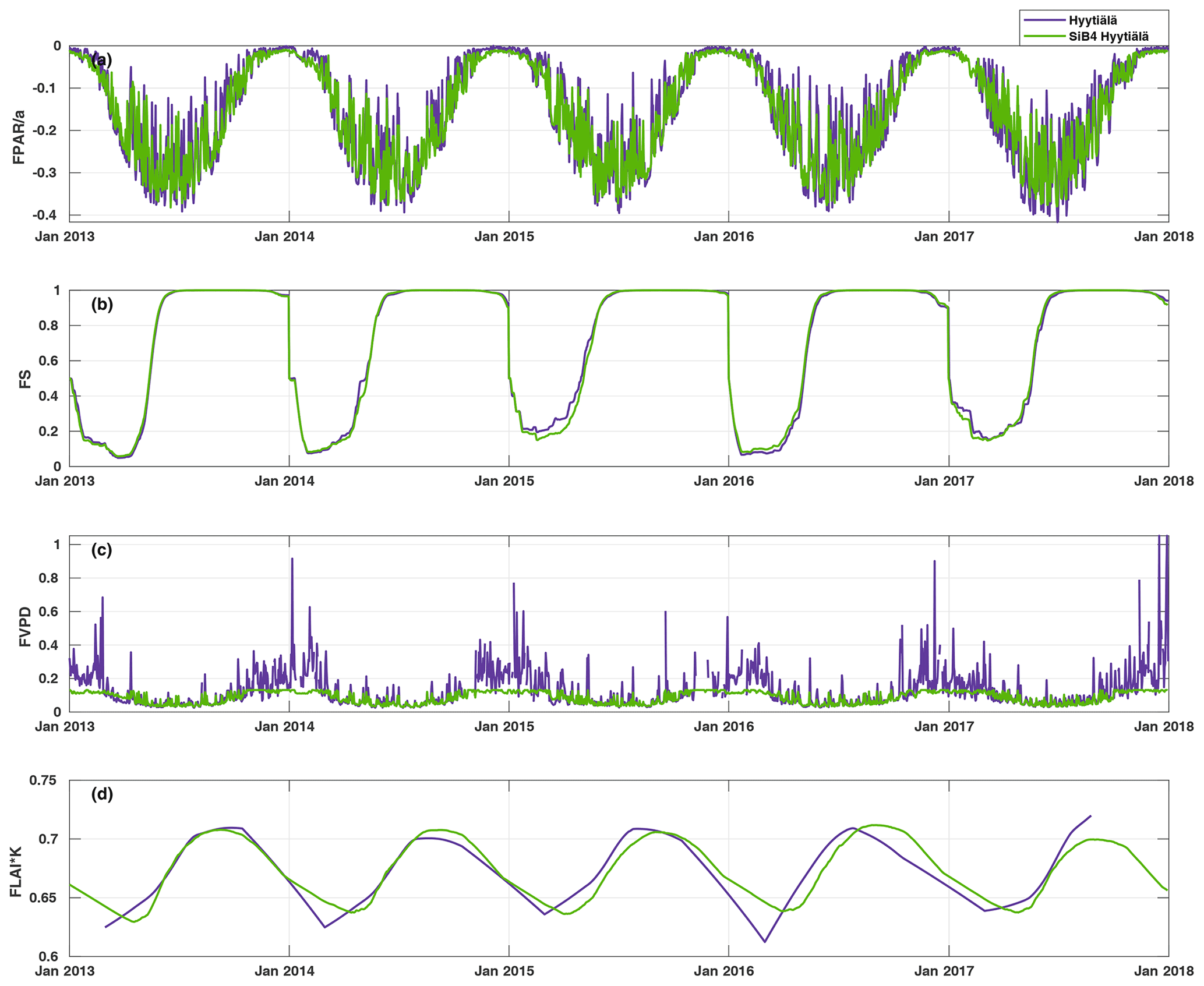
Figure 4Time series of the daily average values of the parameter functions (Eqs. 2–5) normalized to vary between zero and one. The purple line represents the parameterization, and the green line represents the parameterization with SiB4 in Hyytiälä. The abbreviations used in the figure are as follows: FPAR – stomatal response to PAR, FS – phenology of biochemical reactions, FVPD – stomatal regulation, and FLAI – foliage and canopy light penetration.

Download

3.4 Parameterization and simulation of the net carbonyl sulfide flux

Figure 4 presents the modulation of the four variables of the FCOS, where FPAR and FS have the biggest effect (via PAR and T_a governing seasonality), and LAI has the smallest effect. For the dependencies of the parameterization functions (Eqs. 8–11) on their drivers, see Fig. S7. At the same time, PAR varied between 0 and 1870 $\mathrm{\mu }\mathrm{mol}{\mathrm{m}}^{-\mathrm{2}}{\mathrm{s}}^{-\mathrm{1}}$, T_a varied between −28 and +29 ^∘C, VPD varied between 0 and 2.7 kPa, and LAI varied between 5.3 and 7.1 m² m⁻². Equation (7) provides a robust description of the average FCOS dynamics from a yearly to daily scale (R²=0.57) (Figs. 2a and 5 and Figs. S8 and S9, respectively). The difference of the parameterization from the gap-filling function presented in Kohonen et al. (2020) is that, unlike the gap-filling function, this simple parameterization does not require the evaluation of parameter values against measurements every 2 weeks. The evolution of the FCOS is taken into account solely with environmental variables. The prediction from Eq. (7) differs from the monthly medians, with at least 20 % of data measured (filled circles in Fig. 2a), mostly in April–June 2013, July–August 2014, and September 2015. In 2016–2017, the predicted values closely follow the measured data excluding April 2016. In April–June 2013, neither the VPD nor SWC were significantly higher or lower, respectively, than in other years (Fig. S1). In July 2014, the VPD was about twice as high as in 2015–2017; thus, the FCOS were likely low due to stomatal regulation. In April 2015, SWC was lower than in other years, which may also explain the low COS flux in that period. In April 2016, neither the VPD nor SWC were significantly higher or lower, respectively, than in other years. A high VPD or low SWC may also be reflected in the net CO₂ ecosystem exchange (NEE). However, NEE values do not differ from other years during these periods of low COS uptake, excluding the highest carbon uptake (lowest NEE), in contradiction to the FCOS, in July 2014 (Fig. S1). However, PAR was higher in July 2014 than in any other year, which may explain the high carbon uptake. The FCOS are more sensitive to the stomatal conductance than the CO₂ exchange is, because the changes in the sub-stomatal CO₂ concentration partly buffer the direct effect of the stomatal closure.

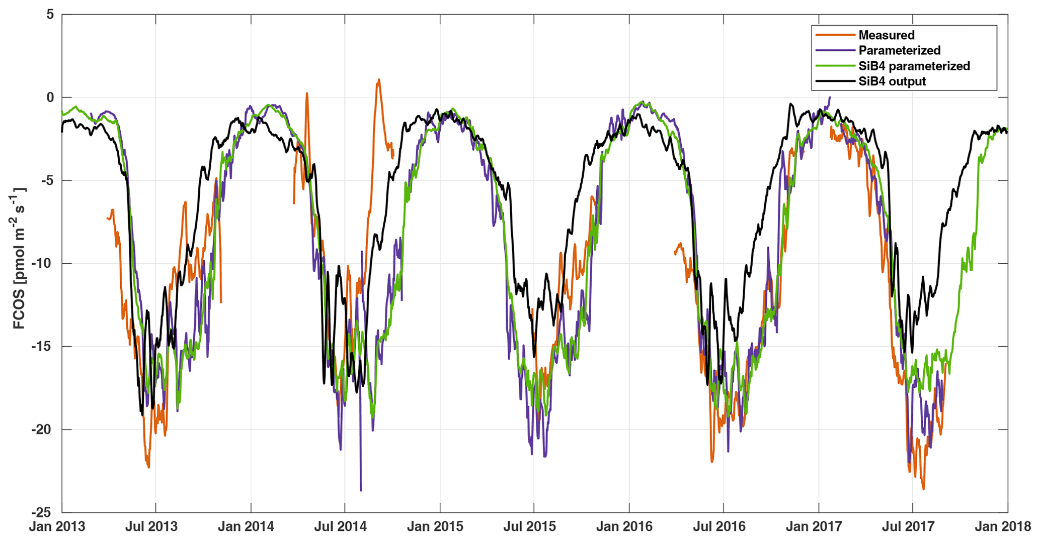
Figure 5Weekly averaged FCOS from measurements (gap filled, orange line), parameterization (purple line), SiB4 parameterization (green line), and standard SiB4 output (black line) in Hyytiälä.

Download

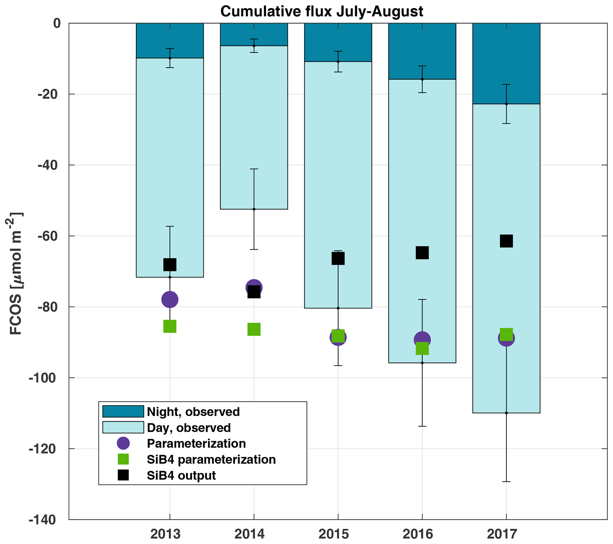
Figure 6Cumulative sum of the gap-filled carbonyl sulfide flux (FCOS) in 2013–2017 during the July–August period, separated into day and night contributions. The percentage of gap-filled COS data during nighttime and daytime, respectively, was 77 % and 58 % in 2013, 70 % and 45 % in 2014, 57 % and 38 % in 2015, 65 % and 43 % in 2016, and 55 % and 29 % in 2017. Purple circles represent the parameterized FCOS, green squares represent the parameterization by SiB4, and black squares represent the standard SiB4 output for Hyytiälä.

Download

Figure 7Daily average (avg) carbonyl sulfide flux (FCOS) in the boreal region based on SiB4 (a, b) and upscaled parameterization simulations (c, d) for the April–October and November–March periods. The boreal region is defined as the area where evergreen needleleaf forests cover more than 30 % of the land area in the Northern Hemisphere.

The local parameterization and the parameterization with SiB4 data are close to each other, whereas the SiB4 simulation underestimates the FCOS, especially during summertime and fall (Fig. 5). Moreover, the decrease in the FCOS that was observed in July–August 2014 due to warm and dry conditions was not simulated by SiB4. Instead, SiB4 simulated larger FCOS than other years (Figs. 5, 6) as a result of higher temperatures. It is likely that SiB4 simulations lack a stomatal response to dry conditions, specifically for ENF. A similar result was found for CO₂ fluxes by Smith et al. (2020), who carried out a study on the European drought in the summer of 2018. They demonstrated that SiB4 does show a drought response but that site observations – specifically in ENF ecosystems – showed a stronger decline in carbon uptake than that from SiB4. In SiB4, ENF is specifically set to be resilient to droughts by setting a lower limit to soil moisture stress on photosynthesis, which is used to derive the stomatal conductance; thus, this setting controls the COS leaf uptake. The COS flux time series provide additional evidence that the lower bound on soil moisture stress in ENF ecosystems should be removed. Regarding the general underestimation of the FCOS by SiB4, Kooijmans et al. (2021) also found that underestimations of the FCOS at Hyytiälä were consistent with underestimations of gross primary production. A possible method to increase these fluxes in SiB4 is to increase the maximum carboxylation rate of RuBisCO that is also used to simulate the carbonic anhydrase activity, which is relevant for COS uptake. Another approach is to incorporate a CO₂ fertilization effect that would increase the aboveground biomass and would also increase both fluxes. Research into the implementation of an accurate representation of the CO₂ fertilization effect in SiB4 is ongoing, and other processes, such as respiration and water use efficiency, are also concurrently being assessed. Simulations of COS soil uptake in Hyytiälä are also too low (Kooijmans et al., 2021), which could be improved with more accurate carbonic anhydrase uptake parameters specific to ENF soil. Several studies have also suggested the role of bryophytes (Gimeno et al., 2017) and epiphytes (Rastogi et al., 2018), which may play a role in boreal forests but which are not specifically included in SiB4.

3.5 Carbonyl sulfide balances and their interannual variation

We analyzed COS balances, the share between day- and nighttime uptake, and their interannual variability. The cumulative FCOS (FCOS_cum) values are presented in Fig. 6 for the periods with the smallest amount of gap-filled data, i.e., July–August in 2013–2017. The FCOS_cum value in 2014 was 52 % lower than in 2017. The larger total uptakes were not only due to daytime uptake. The higher absolute nighttime uptake corresponded not only to the higher total uptake but also to the higher nocturnal percentage of the total uptake. The cumulative nocturnal uptake fraction of the total uptake was 0.14, 0.12, 0.15, 0.17, and 0.21 for the years 2013, 2014, 2015, 2016, and 2017, respectively. The total FCOS_cum values for the period from April to August were $-\mathrm{183}\pm \mathrm{41}$, $-\mathrm{130}\pm \mathrm{30}$, $-\mathrm{207}\pm \mathrm{45}$, and $-\mathrm{205}\pm \mathrm{45}$ µmol COS m⁻² for the years 2013, 2014, 2016, and 2017, respectively. Expressed as sulfur uptake, the FCOS_cum values become $-\mathrm{58.5}\pm \mathrm{13}$, $-\mathrm{41.6}\pm \mathrm{9.6}$, $-\mathrm{66.4}\pm \mathrm{14.4}$, and $-\mathrm{65.5}\pm \mathrm{14.4}$ g S ha⁻¹ for the years 2013, 2014, 2016, and 2017, respectively. We can compare the amount of sulfur deposited by COS with the dominant sulfur compounds. The annual sulfur deposition of sulfate and sulfur dioxide (SO₂) is estimated to be 780 g S ha⁻¹ (Hannele Hakola, Finnish Meteorological Institute, personal communication, 2020) for the measurement site. Thus, the COS sulfur deposition reported here was 7 % of that of sulfate and SO₂. The parameterized FCOS_cum values (both using local meteodata and SiB4 meteodata) show higher total uptake than the FCOS measurements for the years from 2013 to 2015 but lower uptake for the years 2016 and 2017 (Fig. 6). While both the measured and parameterized FCOS_cum have a slight decreasing trend during 2013–2017 (increasing uptake), the SiB4 output shows an opposite trend of increasing FCOS_cum (decreasing total COS uptake). However, this time series is too short to analyze trends, and the observed differences can be explained by differences in environmental drivers.

3.6 Implications for global biogeochemical cycles

The long-term time series presented in this study, as well as the relationships of the FCOS with PAR, T_a, VPD, and LAI, can help to evaluate and improve biosphere models, thereby contributing to an accurate biosphere sink estimate. We calibrated the SiB4 PAR, LAI, VPD, and T_a for the grid cell where Hyytiälä is located against observations (see Fig. S10). We then applied the FCOS parameterization to the calibrated SiB4 meteorological and phenological data for the whole boreal region to evaluate the FCOS simulations using SiB4. The resulting daytime average FCOS values in the boreal region are always larger than the FCOS simulated by SiB4, especially in the summer months (Figs. 5–7, see Fig. S11 for the difference between the two methods). The total FCOS value of evergreen needleleaf forests (ENFs) in the boreal region is estimated to be −14.6 Gg S yr⁻¹ by the parameterization for the years 2013–2017, which is close to the estimate for boreal forests (19.2–33.6 Gg S yr⁻¹) from Sandoval-Soto et al. (2005), but 1.5 times larger than that simulated by SiB4 (−10.6 Gg S yr⁻¹). These results are in line with the recent top-down studies of the COS atmospheric budget (Ma et al., 2021; Remaud et al., 2021; Hu et al., 2021), which have pointed to a missing sink in the higher latitudes of the Northern Hemisphere. The parameterization presented here could serve to improve the prior descriptions of the COS biosphere flux used for inverse modeling studies such as that of Ma et al. (2021). Such an approach would provide more accurate COS biosphere sink estimates and could also help to improve the representation of gross primary production in biosphere models.