the Creative Commons Attribution 4.0 License.
the Creative Commons Attribution 4.0 License.
 | 21 Sep 2021
The role of emission reductions and the meteorological situation for air quality improvements during the COVID-19 lockdown period in central Europe
Volker Matthias
Markus Quante
Jan A. Arndt
Ronny Badeke
Ronny Petrik
Josefine Feldner
Daniel Schwarzkopf
Eliza-Maria Link
Martin O. P. Ramacher
Ralf Wedemann
The lockdown measures taken to prevent a rapid spreading of the coronavirus in Europe in spring 2020 led to large emission reductions, particularly in road traffic and aviation. Atmospheric concentrations of NO2 and PM2.5 were mostly reduced when compared to observations taken for the same time period in previous years; however, concentration reductions may not only be caused by emission reductions but also by specific weather situations.
In order to identify the role of emission reductions and the meteorological situation for air quality improvements in central Europe, the meteorology chemistry transport model system COSMO-CLM/CMAQ was applied to Europe for the period 1 January to 30 June 2020. Emission data for 2020 were extrapolated from most recent reported emission data, and lockdown adjustment factors were computed from reported activity data changes, e.g. Google mobility reports. Meteorological factors were investigated through additional simulations with meteorological data from previous years.
The results showed that lockdown effects varied significantly among countries and were most prominent for NO2 concentrations in urban areas with 2-week-average reductions up to 55 % in the second half of March. Ozone concentrations were less strongly influenced (up to ±15 %) and showed both increasing and decreasing concentrations due to lockdown measures. This depended strongly on the meteorological situation and on the NOx VOC emission ratio. PM2.5 revealed 2 %–12 % reductions of 2-week-average concentrations in March and April, which is much less than a different weather situation could cause. Unusually low PM2.5 concentrations as observed in northern central Europe were only marginally caused by lockdown effects.
The lockdown can be seen as a big experiment about air quality improvements that can be achieved through drastic traffic emission reductions. From this investigation, it can be concluded that NO2 concentrations can be largely reduced, but effects on annual average values are small when the measures last only a few weeks. Secondary pollutants like ozone and PM2.5 depend more strongly on weather conditions and show a limited response to emission changes in single sectors.


The global spread of the coronavirus since the start of 2020 resulted in unprecedented emission reductions caused by lockdown measures in many parts of the world. In Europe, significant reductions in road and air traffic as well as in industrial activities began between the end of February and the middle of March 2020. Emissions were heavily reduced in short time but then steadily increased again as lockdown measures were lifted step by step, until they reached approximately previous-year levels in summer (Forster et al., 2020). However, this temporal emission behaviour varied from country to country and among the different emission sectors. Emission reductions between the second half of March and end of June 2020 were probably the largest in Europe since decades, in particular in traffic. From an air quality perspective, this can be regarded as a huge real-world experiment about the effects of severe emission reductions on air pollutant concentrations and possible side effects of emission reduction measures, e.g. on secondary pollution formation.
Observational data at ground level and from satellite showed large but regionally different reductions in NO2 concentrations (e.g. Bauwens et al., 2020; Menut et al., 2020; Velders et al., 2021; Lonati and Riva, 2021). For particulate matter (PM), concentration reductions were less clear and not necessarily in line with the expectations that would follow the estimated emission reductions. Obviously, weather conditions also have a significant impact on pollutant concentration levels, but despite the high number of publications that analyse COVID-19 lockdown effects on air pollution, meteorological influences are mostly not taken into account properly (Gkatzelis et al., 2021). Wind direction determines strongly the advection of gases and aerosols from distant regions into the area of interest, higher wind speeds can activate additional emission sources like resuspension of deposited particles, solar radiation affects photochemical reactions and precipitation amounts control deposition.
As has been pointed out in recent publications about the effect of COVID lockdown emission reductions on air pollutant concentrations (e.g. Menut et al., 2020; Velders et al., 2021), the relationship between emissions and concentrations is not necessarily straightforward and easy to explain. A simple comparison between before and after lockdown concentrations neglects seasonal and weather effects. A similar argument holds for comparisons with the same week of the previous year. While seasonal effects are considered in this case, the weather situation might still be very different. In addition, technology or economically driven emission changes from one year to another are not taken into account. Chemistry transport models and sophisticated emission models can help in disentangling the relationships between emissions, meteorology and concentration levels. In addition, they can quantify the contribution of different source sectors and investigate effects of reduced concentrations of specific pollutants on the formation of other secondary species. For example, it has been discussed by Kroll et al. (2020) and Huang et al. (2020) that lower NO emissions might lead to higher ozone concentrations and a higher potential for the oxidation of organics, which might result in increased secondary organic aerosol (SOA) formation. In fact, Amouei Torkmahalleh et al. (2021) analysed observed NO2 and O3 concentrations in numerous cities around the world and report increased ozone in urban environments. However, depending on the NOx VOC emission ratios and the meteorological situation, the effects might differ from place to place (see e.g. Mertens et al., 2021).
To quantify the effects of the lockdown measure on ambient concentrations, these need to be separated from other sources of influence which predominantly are assumed to be the meteorological conditions. For Europe, Menut et al. (2020) assessed the influence of lockdown measures on air quality without the biases of meteorological conditions in an ad hoc modelling study for March 2020. They compared a reference model run with 2017 emission data for Europe to a lockdown run with estimated emission reductions. Both runs were based on the same meteorological fields. Considerable decreases in NO2 concentrations due to the lockdown measures alone have been found. The effect on fine particle concentrations has been comparably less pronounced (−5 % to −15 %). Sharma et al. (2020) performed a similar study for India; they reported a remarkable increase in O3. With focus on the Netherlands, Velders et al. (2021) used a machine-learning (ML) algorithm to remove the effects due to meteorological variability on pollutant concentrations and applied chemical transport modelling. They concluded that the unusual 2020 meteorology in the Netherlands led to decreased PM10 and PM2.5 concentrations but the NO2 and O3 concentrations were not affected. In a study addressing the air quality during the lockdown period in Milan, Collivignarelli et al. (2020) eliminated the influence of weather phenomena on the air quality by identifying a meteorological reference period. Using machine-learning (ML) models fed by meteorological data, Petetin et al. (2020) estimated the NO2 mixing ratios for Spain that would have been observed in absence of the lockdown. It was found that the lockdown measures were responsible for a 50 % reduction in NO2 levels. Goldberg et al. (2020) showed that accounting for meteorological influences is important when satellite data are used to estimate the drops in columnar NO2 in the United States. And van Heerwaarden et al. (2021) used ground-based and satellite observations in combination with radiative transfer modelling to disentangle meteorological effects and those of aerosol emissions. They concluded that lockdown measures were far less important for the irradiance record than the exceptionally dry and particularly cloud-free weather.
In this paper we present results derived with the COSMO-CLM/CMAQ model system together with a highly modular emission model to quantify the contribution of the estimated emission reductions on the concentrations of NO2, O3 and PM2.5 in central Europe and to separate the contribution of emission changes from those caused by distinct weather patterns. CMAQ was fed with updated emission data for the year 2020, including time profiles for sectors and countries that approximate the lockdown emission reductions. Chemistry transport model simulations were performed for January–June 2020. The effects of distinct weather patterns on the effects of emission reductions on pollutant concentrations were investigated through additional simulations with meteorological conditions for the same time period in recent previous years with very different weather conditions. The results allow for an interpretation of the observed concentration reductions when compared to previous years. It also gives a range of possible concentration changes resulting from the same emission reductions.
This study focuses on the effects of emission reductions during the lockdown in central Europe in spring and early summer 2020. While emission changes were considered for all of Europe, the main area under investigation with respect to effects on concentrations covers the most populated regions in central Europe (Fig. 1) only. This restriction was applied for the sake of a higher resolution and for allowing a reasonable interpretation of meteorological impacts. The Community Multiscale Air Quality Model (CMAQ) (Byun and Schere, 2006; Byun and Ching, 1999) version 5.2 was used with the carbon bond 5 (CB05) photochemical mechanism (CB05tucl) (Kelly et al., 2010) and the AE6 aerosol mechanism. The model was run for 2020 with a spin-up time of 2 weeks in 2019 to avoid the influence of initial conditions on the modelled atmospheric concentrations. CMAQ was set up on a 36 × 36 km2 grid for all of Europe and for a one-way nested 9 × 9 km2 grid for central Europe; see Fig. 1. The vertical model extent comprises 30 layers from the model surface up to the 100 hPa pressure level. Twenty of these layers are below approx. 2000 m, and the lowest layer has a height of 36 m.
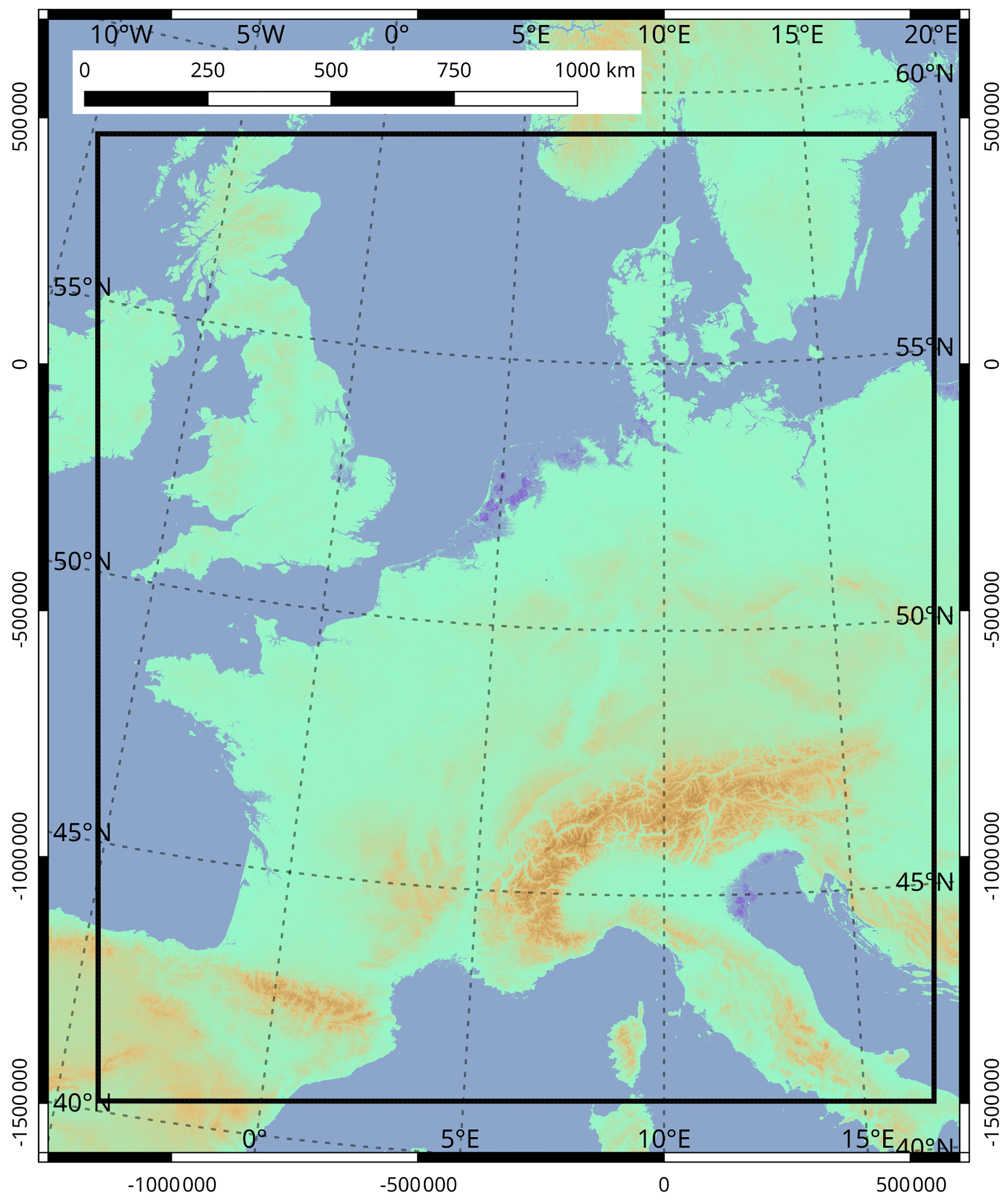
Figure 1Inner domain of the CMAQ model (black line) along with the coordinates of the CMAQ projection (values outside the zebra frame).
Chemical boundary conditions for the outer model domain were taken from the IFS-CAMS analysis (Inness et al., 2019) available from the MARS archive at ECMWF and the Copernicus Atmosphere Monitoring Service Atmosphere Data Store (https://ads.atmosphere.copernicus.eu/cdsapp#!/dataset/cams-global-reanalysis-eac4?tab=overview, last access 16 September 2021). Particle and gas concentration fields of the Global Analysis and Forecast are provided on a T511 spectral grid with 137 vertical levels. Emission changes caused by lockdown measures are not considered in this data set. The IFS-CAMS data were temporally and spatially remapped onto the boundary of the CMAQ domain. Finally, a unit conversion and a transformation of the chemical species from IFS-CAMS to CMAQ were applied.
Meteorological data for the CMAQ model were provided by a simulation of the COSMO model (Baldauf et al., 2011; Doms et al., 2011; Doms and Schättler, 2002) applying the version COSMO5-CLM16 (climate mode; Rockel et al., 2008). To simulate the radiative transfer as realistic as possible, an extension of the COSMO model for the MACv2 transient aerosol climatology was used. The soil was initialized taking the data from a 40-year simulation with the COSMO model. Then, the atmospheric simulations were performed for the period 1 September 2019 to 30 June 2020 using the MERRA2 global reanalysis (Gelaro et al., 2017) as initial and lateral boundary conditions. The same was done for the periods 1 September 2015 to 30 June 2016 and 1 September 2017 to 30 June 2018. To ensure that the atmospheric fields in the transient model integration are close to the observations over the whole period of 10 months, a nudging technique was used as described in Petrik et al. (2021). The reader is referred to this publication to find more information about the setup of the atmospheric model (setup “CCLM-oF-SN”).
CMAQ simulations were performed with emissions as they could be expected for 2020 without any lockdown measures and with another emission data set that was modified according to reported changes in traffic and industrial activities. The latter is regarded as the emission data set that best reproduces real-world emissions during the first COVID-19 lockdown phase in 2020. In the following we will refer to this simulation as the COV case, while the simulation with expected emissions without lockdown is referred to as the noCOV case. The difference between the simulated pollutant concentrations for the two cases represents the COVID-19 lockdown effects on air quality. A detailed description of the emission data construction is given in the next section. Additional model simulations with meteorological conditions for the years 2016 and 2018 have been performed with CMAQ using the same 2020 emission data sets.
3.1 Basic emissions 2020, noCOV case
Emissions are based on the CAMS-REGAP-EU version 3.1 available at the ECCAD website (https://permalink.aeris-data.fr/CAMS-REG-AP, last access: 16 September 2021). The data set comprises annual totals for anthropogenic emissions in 13 GNFR sectors (Granier et al., 2019). The most recent data set was for 2016. For this study, the emission data were extrapolated to the year 2020 based on the temporal emission development in previous years.
For the application in the CMAQ model the data were re-gridded and vertically and temporally redistributed. Additionally, in order to investigate the effects of lockdown measures on the emissions, sector- and country-specific temporal profiles of lockdown effects were applied. The data preparation was done with a modular toolbox for emission calculation, the Highly Modular Emission MOdel (HiMEMO), currently developed at Helmholtz-Zentrum Hereon. The framework is built in the R programming language, using the libraries netcdf, proj4, sp, raster and their dependencies.
HiMEMO was run with gridded emission data from the CAMS inventory for 2016 in a spatial resolution of 0.05∘ × 0.1∘. The inventory contains gridded annual emissions for chemical species groups, i.e. NOx, NMVOC, CO, NH3, CH4, SO2, PM2.5 and PM10. Several of these chemical groups need to be split into chemical components or sub-groups of species according to the CB05 chemical mechanism used by CMAQ. The NOx split was done by applying a NO NO2 ratio of for traffic, a ratio of for shipping and for all other sectors. Land-based NMVOC emissions were split for individual sectors according to a split provided by the Netherlands Organisation for Applied Scientific Research (TNO; Jeroen Kuenen, personal communication, 2020). PM was split as described by Bieser et al. (2011a) for the SMOKE for Europe emission model. All other species in the CAMS-REGAP-EU inventory were directly transferred to CMAQ.
Vertical emission distributions per sector follow Bieser et al. (2011b). The vertical distribution for the shipping sector was treated differently for land and ocean-going ships, with the latter being emitted at altitudes up to 100 m. The temporal profiles follow those provided by TNO (Denier van der Gon et al., 2011, also described in Matthias et al., 2018).
Biogenic emissions of VOCs (BVOCs) and NO were calculated with the Model of Emissions of Gases and Aerosols from Nature (MEGAN) (Guenther et al., 2012). Version 3 of MEGAN (Guenther et al., 2020) was used in this study; it was driven by preprocessed meteorological data for CMAQ as described above. Vegetation data tables were downloaded from the MEGAN website and not further modified for this study. Leaf area index (LAI) data were taken from GEOV1 products (SPOT/PROBA V LAI1) as an alternative input for MEGAN3 (Baret et al., 2013).
The annual emission data for 2016 were extrapolated to 2020 for each national emission sector according to the Gridded Nomenclature For Reporting (GNFR) in order to produce expected emissions for 2020 without lockdown effects. The starting point was the time series data of yearly totals for the pollutants BC, CO, NH3, NMVOC, NOx, PM10, PM2.5 and SO2, which are provided by the EMEP centre on emission inventories and projections (EMEP/CEIP 2020 Present state of emission data; https://www.ceip.at/webdab-emission-database/reported-emissiondata, last access: 16 September 2021). Using the time series data, a mean annual change rate for emissions (CE, in %) was derived for each pollutant, sector and country separately. The projection of the 2016 emissions to the year 2020 was realized through a projection factor PF = 1 + CE 100 × (2020 − 2016). Using a mean change rate based on the development of emissions within the 3 years 2017–2019 (method 1), PF could be very large (more than 2) for some countries and sectors. This can result from large changes and fluctuating time series of the yearly emissions. In order to avoid very large and presumably erroneous emission changes between 2016 and 2020, a maximum allowed annual change rate was introduced. If the CE was larger than 10 %, a modified CE was computed by considering the entire time series of annual emissions but not more than 10 years (method 2). If there still was a CE of more than 10 %, we limited it to a maximum change of ±10 %. Regarding the shipping sector, no changes were assumed between the years 2016 and 2020.
3.2 Lockdown effects, COV case
For the lockdown scenario, we adjusted national emissions from the following GNFR sectors: A_PublicPower, B_Industry, F_RoadTransport, G_Shipping and H_Aviation. Lockdown emission reduction functions, here called lockdown adjustment factors (LAFs), were calculated based on published data sources that resemble the effects of lockdown measures on a daily basis. LAFs were derived for 42 European countries and two sea basins, the North Sea and the Baltic Sea.
The data sets used for the construction of the LAFs are described in the following. If the input data were not available for an individual country, data from a neighbouring country were used to estimate the reduction. A table showing the data availability per sector and country is given in Appendix A (Table A1). The LAFs are applied to all species, heights and time steps of the anthropogenic emission data set for 2020.
3.2.1 A_PublicPower and B_Industry
Eurostat data (https://ec.europa.eu/eurostat/databrowser/view/sts_inpr_m/default/bar?lang=en, last access: 16 September 2021) were used to account for changes in the sectors A_PublicPower and B_Industry. The energy data provided there comprise monthly information on the volume index of production for electricity, gas, steam and air conditioning supply. They are available for 35 countries in Europe. The industry data comprise monthly information on the volume index of production for mining and quarrying; manufacturing; electricity, gas, steam and air conditioning supply; and construction and are available for 20 countries in Europe. The indices are based on an index value of 2015. However, since we want to use them to evaluate the lockdown period, we normalized the changes based on the January 2020 value. The data are given in a monthly resolution; however, for many countries in Europe the lockdown started in the middle of March. Therefore, a piecewise cubic spline interpolation procedure was applied to derive daily lockdown adjustment factors while still maintaining the monthly values. Examples are given for both sectors in Germany in Fig. 2.
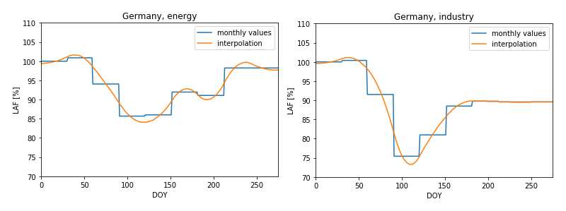
Figure 2Examples for monthly values and interpolated functions for lockdown adjustment factors (in %) for the sectors A_PublicPower and B_Industry in Germany.
3.2.2 F_RoadTransport
Google mobility reports (https://www.google.com/covid19/mobility/, last access: 16 September 2021) deliver daily percentage change of visits in different areas (e.g. residential, transit, recreation, work places). The reference value is the median of the corresponding weekday between 3 January and 6 February 2020. We use Google mobility reports for transit on a national level to account for the changes in road traffic emissions. Through this method, reduced traffic on national holidays, e.g. around Easter and 1 May, is considered as well; however, vehicle types cannot be distinguished.
3.2.3 G_Shipping
To derive scaling factors that account for ship traffic and emission reductions in this sector, bottom-up ship emission inventories were created with the MOSES ship emission model (Schwarzkopf et al., 2021) using automatic identification system (AIS) data for 2019 and 2020 covering the German Bight and the western Baltic Sea. The data were recorded in Bremerhaven and Kiel by the German Federal Maritime and Hydrographic Agency (BSH). A 7 d rolling mean filter was applied to the calculated CO2 emission ratios (Fig. 3). On average, the data revealed a slight reduction of ship traffic in the North Sea area by approx. 10 %. For the Baltic Sea traffic reductions were clearly visible with a downward trend from March until the middle of June that could be mainly attributed to roll-on/roll-off (RoRo) ships and passenger ships. For the first 75 d of the year until 15 March 2020 no reductions were applied; afterwards daily LAFs were used similar to the approach for road traffic. LAFs for the North Sea were also applied for the Mediterranean Sea; those for the Baltic Sea were also applied to inland shipping. The reasoning behind this is that shipping in the Mediterranean is mostly international cargo transport, similar to the North Sea, and inland navigation is connected to short-range transport, similar to the Baltic Sea. As can be seen in Fig. 3, relative increases in shipping emissions might also occur during limited time.

Figure 3Lockdown adjustment factors created from the 7 d rolling mean ratios of CO2 emissions from shipping in 2020 relative to 2019. Until day 75 (15 March) no changes and a LAF of 1 was assumed.
3.2.4 H_Aviation
Airport traffic total arrivals and departures data from Eurocontrol (https://ansperformance.eu/data, last access: 16 September 2021) were used to account for emission changes in the aviation sector. We applied a reduction based on a weekday mean from 3 January until 6 February 2020, similar to Google mobility data. Daily values for 42 European countries are available. The relative reductions in this sector were most pronounced, reaching −90 % in March and April and a slower recovery than the other sectors.
3.2.5 Sector comparison
LAFs for Germany, France, the UK and Sweden are exemplarily shown in Fig. 4. Huge emission reductions in road traffic and air traffic between 10 and 20 March (day of the year (DOY) 70–80) can clearly be seen. Public power and industry, on the other hand, show much smaller reductions (10 %–30 %) and almost reach previous-year levels until the end of June. At the same time in France and Germany, road traffic was back to 90 % of the previous year; however, in the UK and in Sweden 20 %–40 % reductions were still visible in the activity data. Comparisons of country-specific LAFs for the sectors F_RoadTransport and H_Aviation are given in Appendix A (Figs. A1 and A2).

Figure 4LAFs for Germany (a), France (b), the United Kingdom (c) and Sweden (d) for the sectors A_PublicPower, B_Industry, F_ RoadTransport and H_Aviation.
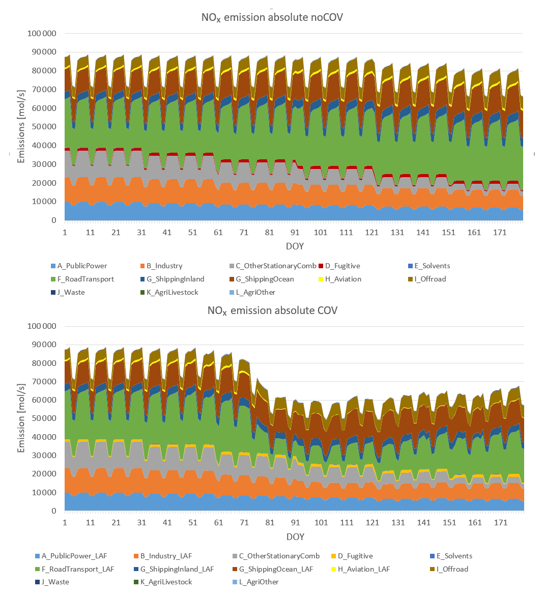
Figure 5Daily average values for sector separated NOx emissions summarized over the entire central European model domain for the noCOV and the COV case (with LAF).
Figure 5 presents total daily NOx emissions in the entire central European domain (see Fig. 1) for the time period from 1 January to 30 June 2020 for the COV and the noCOV case separated by GNFR sectors. Road transport is the most important emission sector with approx. 20 % to 30 %, followed by ocean shipping, other stationary combustion, industry and public power, which all have similar contributions of approx. 10 %. Combustion shows a clear decline towards the summer months due to the fact that domestic heating is mainly necessary in winter.
Reductions caused by the lockdown stem mostly from the road transport sector, with a strong drop in emissions starting around DOY 75 (15 March). The aviation sector, which experienced the strongest relative drop in emissions during the lockdown, does not play a major role for the overall emission of NOx. However, it might be important near airports and in the upper troposphere. Overall, NOx emissions in central Europe dropped by around 25 000 mol s−1 (approx. 4 kt h−1, when given as NO2) during the strictest lockdown period in late March and early April. This corresponds to a relative drop of around 30 % (Fig. 5).
We focus our analysis on the most important air pollutants for human health, namely NO2, O3 and PM2.5. In this chapter, first the meteorological situation between 1 January and 30 June 2020 is analysed. Afterwards, observational air quality data at six selected measurement stations within the EEA network (https://www.eionet.europa.eu/countries/index, last access: 16 September 2021) are presented and discussed.
4.1 Meteorological situation
During the lockdown period in spring 2020 large parts of the region of interest experienced exceptional weather that is assumed to have a strong influence on concentrations of some of the pollutants in focus.
The weather conditions during the first half of the year 2020 show strong variations across the months and a different character in the northern part of our model domain compared to more southern regions like the Po Valley. While in the north February was extremely wet and windy (south-westerly direction), the second half of March and April were very dry and sunny. Thus for meteorological reasons a comparison of pre-lockdown pollutant concentrations with those during the lockdown is fairly meaningless in assessing the effect of lockdown measures on the concentrations in the central and northern part of the region of interest.
To further analyse the weather regimes for the first half of 2020 the classification proposed by Gerstengarbe and Werner (1993) has been chosen (see also Bissolli and Dittmann, 2001). This classification identifies predominant synoptic regimes over central Europe and defines 30 so-called “Großwetterlagen” (GWLs), which can be isolated by an objective method introduced by James (2007). The underlying data for this analysis were provided by the German Weather Service. The results of the GWL classification can be found in Table A2.
4.1.1 Pre-lockdown period
In February 2020, an unusually wet period occurred due to strong cyclonic activity in central Europe. Westerly and north-westerly cyclonic regimes were observed on 76 % of the days, whereas high-pressure-type regimes were observed on only 24 % of the days. Thus, the shortwave downwelling irradiance in February 2020 is one of the lowest measured at the weather station Wettermast Hamburg (53∘31′09′′ N and 10∘06′10′′ E) (https://wettermast.uni-hamburg.de, last access: 5 July 2021) (Brümmer and Schultze, 2015) during the last 25 years (Fig. A4), being representative for north-western Europe. The accumulated precipitation for February at this weather station with an amount of more than 120 mm was exceptionally high compared to the last decades (Fig. A4).
4.1.2 Main lockdown period
For the meteorological characterization of the main lockdown period between the middle of March and the end of April we rely in addition to the GWL analysis on maps of the 500 hPa geopotential height and the surface pressure distribution. The underlying data were extracted from simulations with the COSMO–MERRA system, the same meteorological fields which have been used for the chemistry transport calculations with CMAQ displayed and discussed in the following chapters. In Fig. 6 a subset of those maps for three selected time periods is shown; the complete set of maps generated can be found in Appendix A (Fig. A5). To characterize and quantify horizontal advection, wind roses derived from observations at the Wettermast Hamburg are displayed in Fig. 7. The wind data in each plot cover a time period of about 15 d. Measurements at an altitude of 110 m were chosen to better represent a larger area and eliminate parts of the surface influences on the wind.

Figure 6500 hPa geopotential heights (in geopotential decametres, gpdm) and surface pressure (in hPa) for selected time segments in March and April 2020 according to the COSMO simulations. The geopotential heights are averaged over 4 d (21–24 March, 6–9 April and 21–24 April from left to right, respectively). Displayed surface pressure distributions are representative snapshots within those time segments.
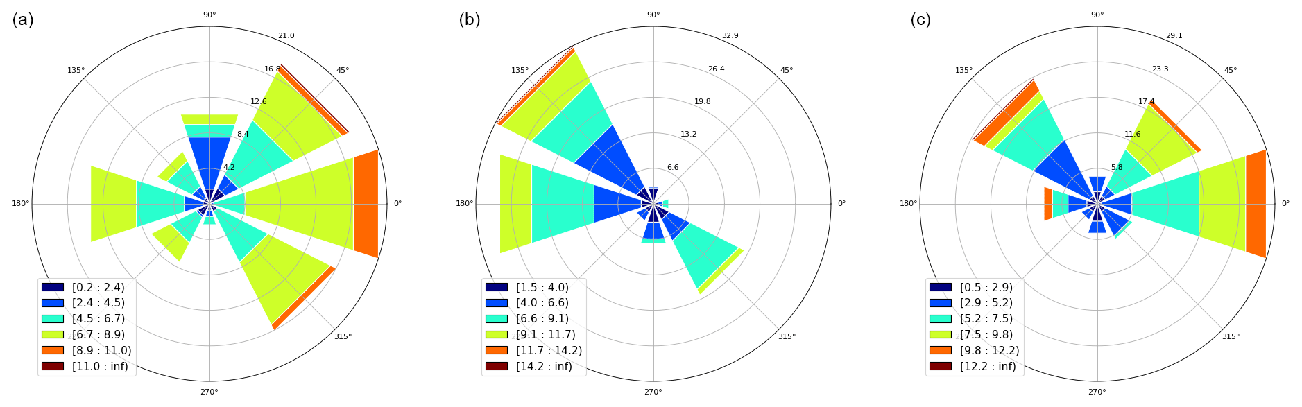
Figure 7Wind roses derived from measurements of the weather station Wettermast Hamburg at an altitude of 110 m. Results for three periods covering about 15 d each are shown: 16–31 March 2020, 1–15 April 2020 and 16–30 April 2020, from left to right.
In the middle of March, the synoptic regime substantially changed over Europe. High-pressure-type GWLs became dominant; i.e. high ridges over central Europe and high-pressure systems led to a typical atmospheric blocking of cyclones. The weather situation shows first a varying blocking in northern and central Europe followed by a high-pressure ridge reaching from the Azores to Scandinavia (Fig. 6, left), which changed to a high-pressure ridge stretching from Iceland into Russia. In northern Germany the wind regime was dominated by a flow with mainly easterly components, which were relatively high wind speeds (Fig. 7, left). In southern Europe the situation, which was similar at the beginning of the period to that one in the north, with changes starting on about 23 March, an isolated trough formed, leading to low-pressure system activity. For 28 and 29 March dust transport from Asia and Northern Africa to the Po Valley was reported (Collivignarelli et al., 2020).
In the first half of April the weather in the north-eastern part of central Europe was again quite variable, and in southern Europe the cut-off from the northern regime could still be recognized. In the western part of central Europe a ridge has established, which stretched towards the UK. Accordingly, winds in northern Germany blew predominantly from westerly/north westerly directions. Later on, a ridge over all of central Europe dominated the weather in the study domain (Fig. 6, middle), only the eastern Mediterranean was still influenced by a cut-off trough. In the Po Valley, according to measurements around Milan, the weather during the second half of March to 10 April was dry and very sunny with low to medium wind speeds (Collivignarelli et al., 2020). Towards the middle of April a high-pressure bridge was established reaching from Iceland into eastern Europe.
In the second half of April a high-pressure system established over the British Isles attached to a ridge located over central Europe leading to dry and sunny weather all over Europe. This condition was basically stable until 25 April, when a cyclonic flow took over, leading to more westerly winds over central Europe, a situation which lasted until the first days of May. Winds in northern Germany switched over from easterly to more westerly directions this time (Fig. 7, right).
Overall, an exceptionally dry period occurred which started in the early lockdown period and continued until the end of April. The weather was characterized by very low cloud cover and record-breaking large amounts of solar irradiance (see the record at the Wettermast Hamburg in Fig. A4) and little precipitation. This exceptional weather period is also discussed by van Heerwaarden et al. (2021), who reported record breaking solar irradiation for the Netherlands.
4.1.3 Lockdown transition
In May 2020, atmospheric conditions were very different in central Europe compared to the previous months. For instance, Germany was dominated by large amounts of rain in the south, sunny conditions in the west, and dry but cloudy conditions in the east and north. Observed sunshine duration and solar irradiance corresponds approximately to average climatic conditions. In contrast, large parts of western Europe (the Netherlands, Belgium, West Germany, the UK) experienced sunny and dry weather throughout the entire month of May (van Heerwaarden et al., 2021). Finally, the large-scale conditions in June turned out to favour long-lasting periods with dry and sunny weather conditions in northern Germany due to blocking conditions caused by high-pressure systems located over Scandinavia. However, the more southerly regions were rather too wet in a climatological sense.
4.2 Concentrations of NO2, O3 and PM2.5
The reduced emissions of pollutants during the lockdown periods should lead to changes in ambient concentrations of those substances and related secondary pollutants as ozone. Beside regional emissions advected pollutants and the meteorological conditions also determine local and regional concentrations. To assess changes in air quality and alterations in the behaviour and nature of concentration, time series observations at selected air quality measurement stations have been examined. The analysed stations have been selected in a way that they are geographically distributed over the study domain and represent different emission characteristics. The stations Radhuset in Malmö, Sweden, and Sternschanze in Hamburg, Germany, are classified as urban background stations, not directly influenced by traffic. Waldhof is a rural background station in northern Germany located about 60 km north of the city of Hanover. Vredepeel is a background station in a fairly populated part of the Netherlands situated in the triangle between the cities Nijmegen, Eindhoven and Venlo. The observatory Košetice in the Czech Republic is located in the Moravian Highlands in an agricultural countryside about 80 km from the south-east of Prague. To represent a region south of the Alps the Italian station San Rocco in the Po Valley about 30 km east of Parma has been selected. With the exception of Košetice, having an elevation of about 530 m, the stations are situated below an altitude of 80 m. To allow a comparison of the concentration measurements under different meteorological influences, time series of NO2, O3 and PM2.5 for the years 2015 to 2020 have been examined. However, PM2.5 was not available at the station San Rocco.
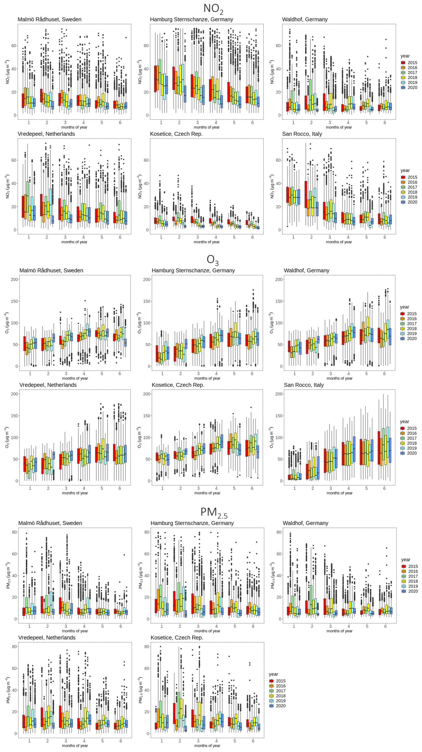
Figure 8Observed monthly concentrations of NO2, O3 and PM2.5 at Waldhof (Germany), Vredepeel (the Netherlands), San Rocco (Italy), Košetice (Czech Republic), Malmö (Sweden) and Hamburg (Germany). The median is displayed within the central boxes which span from the 25th percentile to the 75th percentile, called the interquartile range of the underlying frequency distributions. For NO2 and PM2.5 these distributions are based on hourly measurements at the different stations and for O3 on daily 8 h maximum values. The whiskers above and below the central boxes indicate the largest and the smallest value within 1.5 times the interquartile range, respectively. Dots denote values outside these ranges. PM2.5 was not available at San Rocco.
The observational results for the selected stations for NO2, O3 and PM2.5 are displayed in Fig. 8. For NO2, at all stations, with the exception of Waldhof, an obvious trend from higher concentrations in the winter months to lower ones in spring in early summer can be seen. At Waldhof this trend is not that clear due to lower values in January for most of the years. As it can be expected, in urban (Malmö and Hamburg) or densely populated (Vredepeel and San Rocco) regions the NO2 concentrations are on a higher level. At most stations the NO2 concentrations for March 2020, the month during which in all countries the lockdown measures started, are among the lowest ones compared to the previous years. For Hamburg, Vredepeel and Košetice this also holds for the months April to June. An obvious feature, which appears at all stations except San Rocco, is that the February concentrations in 2020 are lower compared to the previous years, although no lockdown measures were taken in Europe in February. Presumably, meteorological conditions are responsible for these relatively low NO2 concentrations. February 2020 was a month with steady westerly winds and longer periods of intense precipitation in northern Europe. While strong winds cause rapid dilution of pollutants, steady precipitation has a cleaning effect due to dissolution of pollutants in cloud and rainwater and subsequent washout.
For O3, at all stations and for all years the typical trend from low winter concentrations to higher concentrations in spring and early summer can be seen. During the lockdown month April the O3 concentrations for the years 2018, 2019 and 2020 were higher than in the previous years. During those years the radiation was rather intense in April, which favours the photochemical formation of ozone. At the rural stations Waldhof and Košetice ozone concentrations in May and June 2020 were lower than in previous years. At the urban stations in Malmö and Hamburg the relative increase in O3 concentrations over the 6-month period is lower compared to the more rural stations. This can be interpreted as a titration effect of O3 by reactions with NO, which has significant sources in urban areas. In general, the observations of O3 maxima do not provide any indication of significant effects related to lockdown emission changes in 2020.
PM2.5 concentrations also show no clear signal that would allow us to relate concentrations to lockdown emission reductions. Slightly higher concentrations and variability can be observed in winter compared to summer at all stations. This can be related to the fact that very high PM concentrations appear in winter, only, when emissions are high and atmospheric mixing is suppressed, e.g. during high-pressure situations with advection of cold air. Similar to the NO2 concentrations, rainy and windy weather in February 2020 leads to low PM2.5 concentrations at all stations.
4.3 Model results at measurement stations
In order to judge the quality of the model results, simulated concentrations were compared to observations at selected stations, including some of those presented above. Figure 9 exemplarily shows the comparison at Vredepeel, and Table 1 contains statistical values for NO2 and O3 at 11 stations and for PM2.5 at 4 stations in Europe.
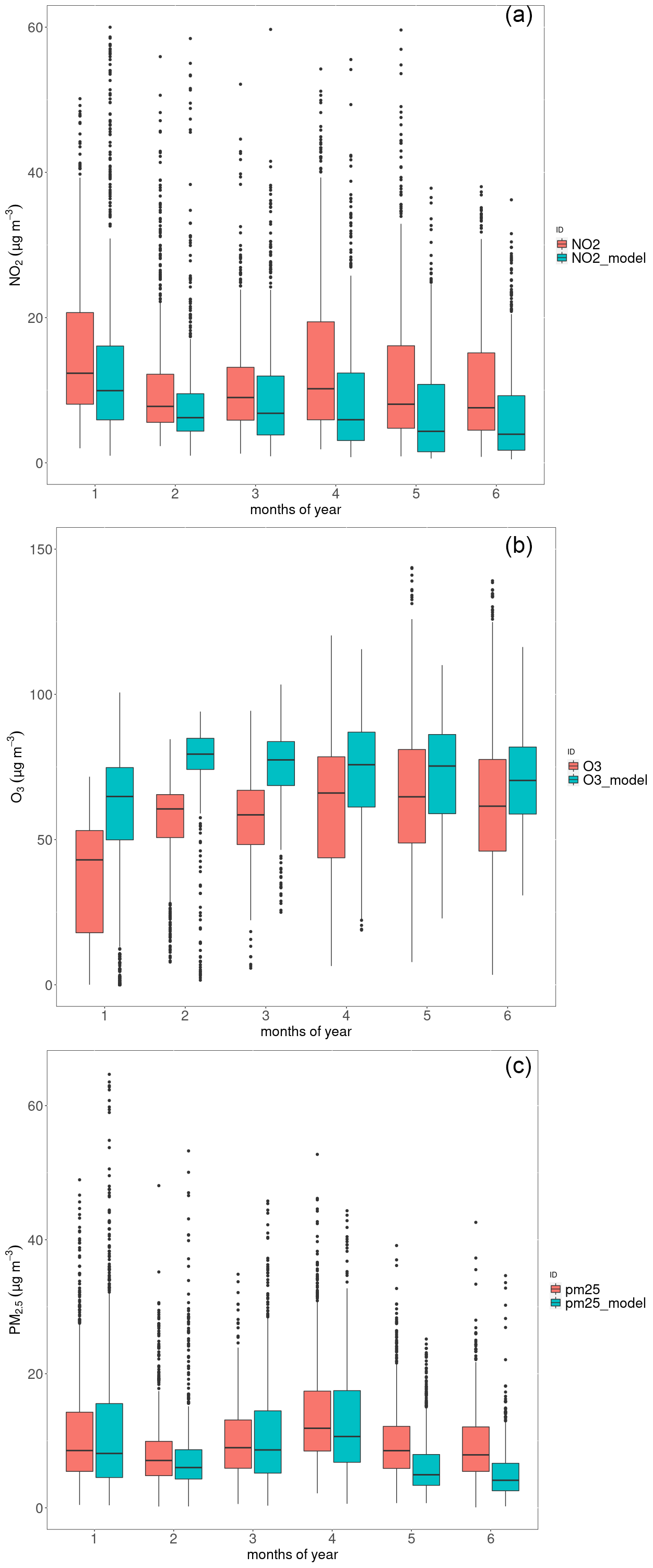
Figure 9Comparison between model results (green) and observations (red) at Vredepeel, the Netherlands. (a) NO2, (b) O3 and (c) PM2.5. All concentrations are given in µg m−3; box plots show medians, 25 % and 75 % quartiles, and whiskers representing 1.5 times the interquartile range. Values that fall outside the range of the whiskers are given as dots.
Table 1Statistical evaluation of a comparison between observations of NO2 at selected background stations of the EEA network with CMAQ model results between 1 January and 30 June 2020.
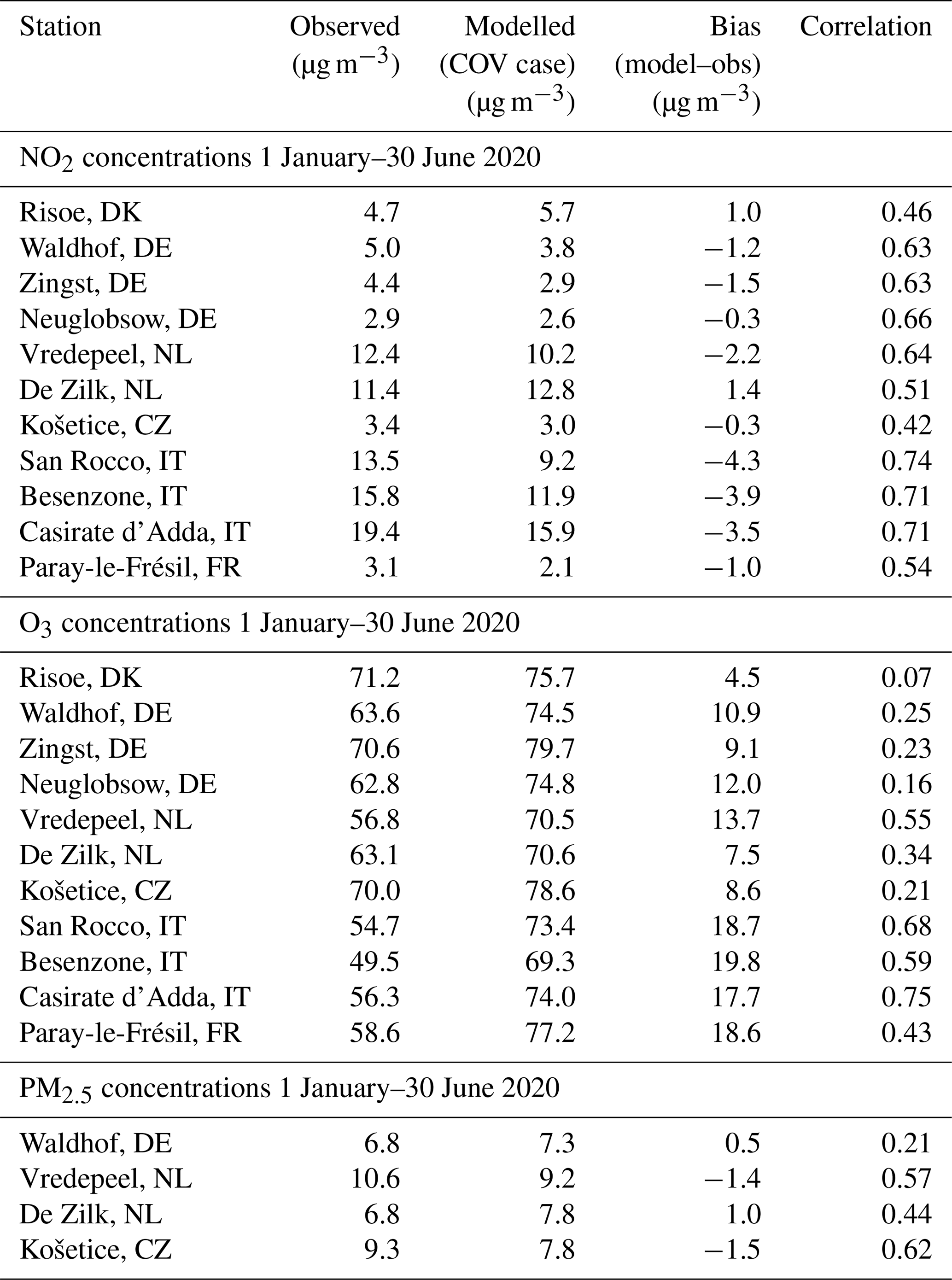
Modelled NO2 concentrations are typically lower than the observed values; in particular, the model shows a stronger downward trend of the concentrations in spring than observed. This pattern is reversed for ozone, where the modelled 8 h max concentrations are typically too high, with better agreement in spring compared to winter. PM2.5 is underestimated on average, but only at two out of four stations. Here, the agreement is typically better in winter compared to spring. As average for all selected stations, the model bias for NO2 is −17 %, for O3 it is +21 % and for PM2.5 it is −5 %. The temporal correlation (R2) based on daily mean values varies between 0.42 and 0.74 for NO2, between 0.07 and 0.75 for O3, and between 0.21 and 0.62 for PM2.5. Details are given in Table 1.
Effects of the lockdown measures on emissions were discussed in Sect. 3. Now, CMAQ model results are evaluated for the COV and the noCOV case during the lockdown phase. Meteorological impacts are discussed through comparisons of CMAQ model results that were derived with meteorological data for the years 2016 and 2018.
5.1 CMAQ results for central Europe
Differences between the CMAQ results for 2020 for the COV and the noCOV case reveal the impact of the lockdown emission reductions on air pollutant concentrations. The magnitude of the concentration changes varies considerably in time and space. Here, we focus our evaluation on the period with the highest emission reductions between 16 and 31 March 2020. During this time the most widely spread and temporally stable emission reductions took place in Europe. Differences among weekdays and weekends and, to a limited extent, also among different weather situations are averaged out by investigating a half-month period. However, changing effects over time are also discussed.
5.1.1 NO2 concentrations
Figure 10 shows maps of the modelled average NO2 concentrations in central Europe between 16 and 31 March for the case without lockdown measures (noCOV) together with the absolute and relative concentration reductions caused by the lockdown. The NO2 concentrations for the noCOV case in central Europe show the typical pattern with highest concentrations in densely populated areas like England, Belgium, the Netherlands, and western Germany as well as northern Italy (Fig. 10a). Average concentrations range between 5 and 10 µg m−3. Reductions in NO2 concentrations caused by the lockdown are highest in the same regions, also reaching several µg m−3. Relative reductions are highest in France, Belgium, Italy and Austria, reaching more than 40 % on average. Germany, the Netherlands, the UK, southern Sweden and the Czech Republic show lower reductions between 15 % and 30 %. In the following weeks, NO2 concentrations stayed more or less on the same level in most parts of Europe, but the lockdown effects decreased slightly as it could be expected from the emission changes. Overall, relative concentration reductions were most significant in England, France, Belgium and Italy, as it was seen for the second half of March. Maps for relative reductions due to the lockdown for six half-month periods between 1 March and 31 May 2020 are given in Appendix A (Fig. A6).
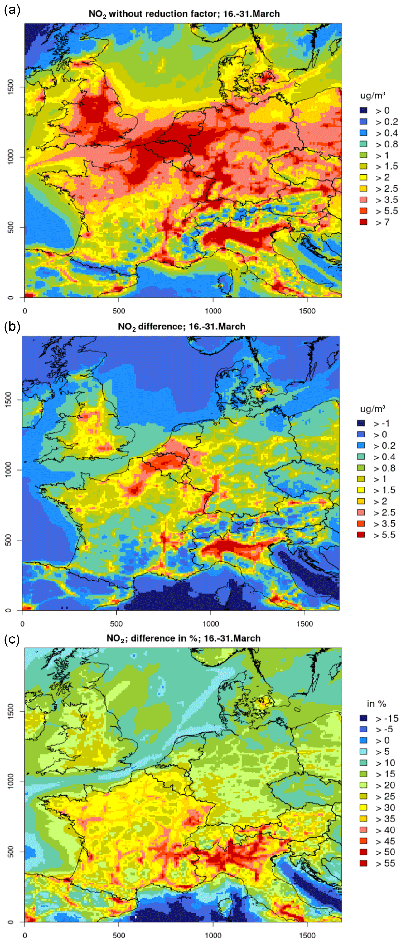
Figure 10CMAQ results for NO2 concentrations in central Europe between 16 and 31 March 2020. (a) Concentrations without lockdown measures (noCOV run). (b) Absolute concentration reductions due to lockdown measures (noCOV – COV run). (c) Relative concentration reductions due to lockdown measures (noCOV – COV run). Positive values for absolute and relative differences denote high reductions.
5.1.2 O3 concentrations
It can be expected that reduced NOx emissions are also reflected in modified O3 concentrations with lower values in all regions that are NOx-limited. However, for the second half of March increased O3 concentrations between 1 and 8 µg m−3 were modelled in the COV case for northern central Europe and the Po Valley (Fig. 11). Because these are the regions with the highest NOx emissions in Europe, they were most likely VOC-limited during this first lockdown period, and O3 titration with NO was reduced when NOx emissions were reduced. Most of the southern parts of the modelling domain exhibited a decrease in ozone of 1–2 µg m−3 on average caused by the lockdown and the reduced NOx emissions. In the following weeks, areas with increased ozone turned smaller week by week and were limited to large cities and the most densely populated areas; see Fig. 12 for the first half of April and the first half of May. Most regions in Europe turned into NOx-limited areas in spring 2020, resulting in lower ozone concentrations of 1–2 µg m−3 (about 2 %–4 % change) caused by the emission changes during the lockdown (Fig. A7).
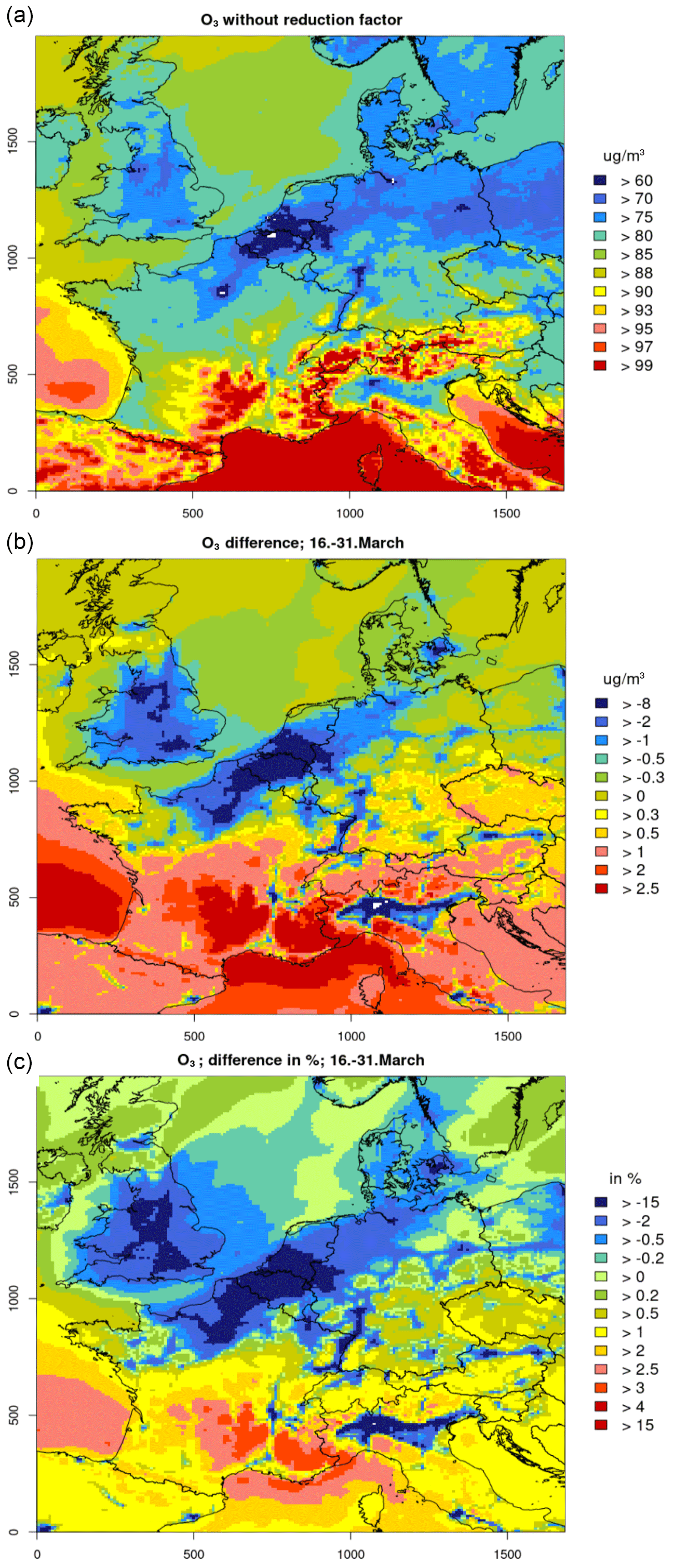
Figure 11CMAQ results for O3 concentrations in central Europe between 16 and 31 March 2020. (a) Concentrations without lockdown measures (noCOV run). (b) Absolute concentration reductions due to lockdown measures (noCOV – COV run); positive values denote high reductions. (c) Relative concentration reductions due to lockdown measures (noCOV – COV run); positive values denote reductions, and negative values denote increases.
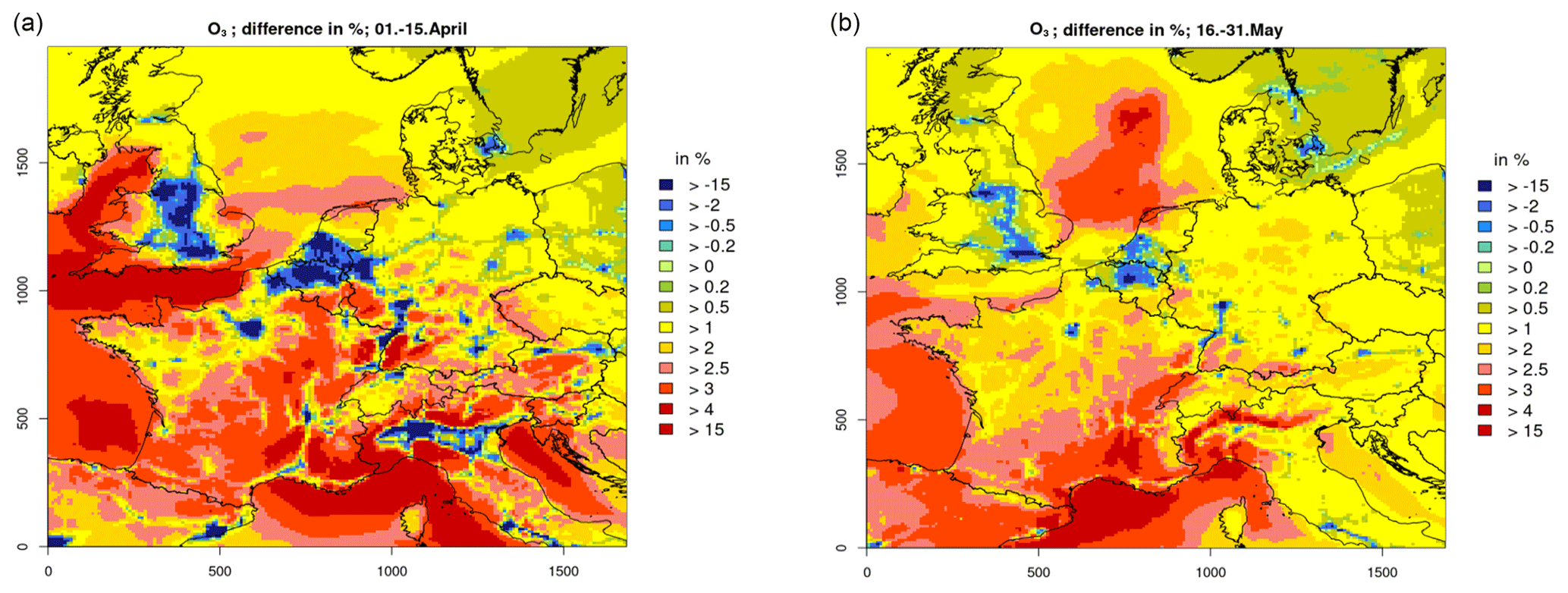
Figure 12CMAQ results for changes in O3 concentrations due to lockdown measures in central Europe between 1 and 15 April 2020 (a) and 16–31 May 2020 (b). Positive values denote concentration reductions, and negative values denote concentration increases.
5.1.3 PM2.5 concentrations
Simulated PM2.5 concentrations in the second half of March 2020 for the noCOV case show relatively high concentrations between 12 and 15 µg m−3 in large parts of central Europe and the Po Valley, while the UK, Denmark and northern Germany exhibited concentrations below 10 µg m−3 (see Fig. 13, top). The lockdown emission reductions lead to concentration reductions between 1 and 3 µg m−3 in those regions with higher concentrations and values below 1 µg m−3 in the north-western part of the domain. Relative concentration decreases were most significant in France and northern Italy with values up to 20 %, while in the rest of the domain 6 %–10 % lower PM2.5 was simulated. In the following weeks, PM2.5 concentrations were typically reduced by 10 %–20 % because of the lockdown measures in most parts of central Europe. Somewhat lower values were found in the northern and southern parts of the domain. The reduction in PM2.5 concentrations decreased to 6 %–12 % in the second half of May (see Fig. A8).
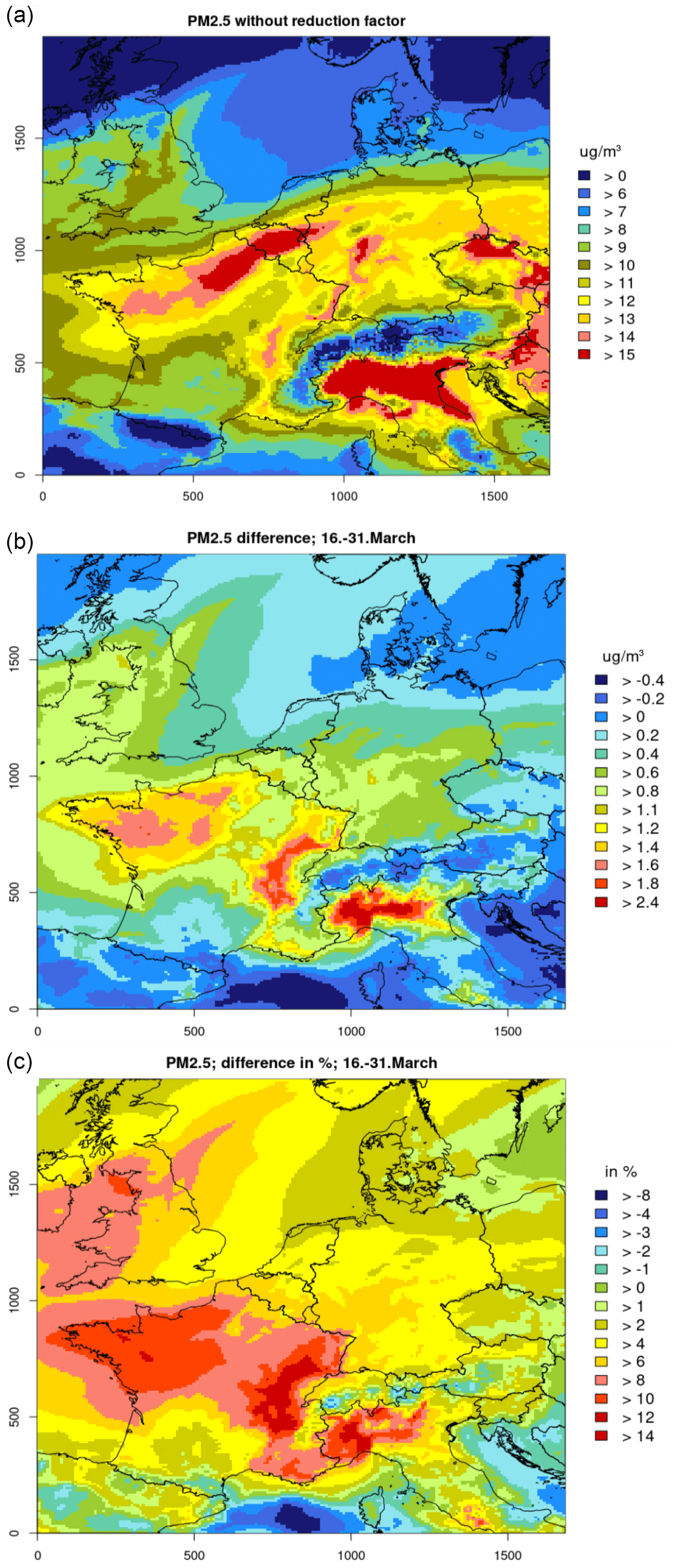
Figure 13CMAQ results for PM2.5 concentrations in central Europe between 16 and 31 March 2020. (a) Concentrations without lockdown measures (noCOV run). (b) Absolute concentration reductions due to lockdown measures (noCOV – COV run); positive values denote reductions. (c) Relative concentration reductions due to lockdown measures (noCOV – COV run); positive values denote reductions.
An investigation of the chemical components of the modelled PM2.5 concentrations for the noCOV case reveals that about two-thirds consists of the inorganic components nitrate (NO), sulfate (SO) and ammonium (NH). The lockdown measures caused large reductions in NOx emissions. Consequently, nitrate was reduced by more than 24 % in large parts of France and northern Italy between the middle of March and the end of April; see Fig. A9 in Appendix A. The reduction was usually somewhat lower in other parts of the domain. Particulate nitrate is mostly bound to ammonium; however, the model results show a lower relative reduction of the ammonium concentrations compared to nitrate. It is only on the order of 8 %–20 % at maximum (Fig. A10). This is because ammonium is preferably bound to sulfate in atmospheric aerosols, and sulfate concentrations even increased by a few percent as a consequence of the lockdown measures (Fig. A11). This can be explained by the large reduction in the formation of particulate nitrate in the COV case. Less nitrate means less ammonium which is then available as gaseous ammonia. This may lead to the formation of additional ammonium sulfate in areas where gaseous sulfuric acid is available.
5.1.4 Temporal development of concentration changes
The detailed temporal development of the effect of lockdown emission reductions on atmospheric concentrations of NO2, O3 and PM2.5 is followed at selected measurement stations. Figure 14 shows the modelled differences between the noCOV and the COV model runs at Waldhof, Vredepeel and San Rocco. Lockdown emission reductions lead to reduced concentrations of NO2 and PM2.5 at all stations; however, the amount varies considerably in time and by station. At Waldhof, only very small changes are simulated. At Vredepeel, NO2 is significantly reduced (by more than 10 µg m−3 on individual days), and PM2.5 shows only small reductions. At San Rocco, both NO2 and PM2.5 are reduced by several µg m−3 until the end of April. In May and June, lockdown effects on the concentrations get much smaller, also at Vredepeel and San Rocco.
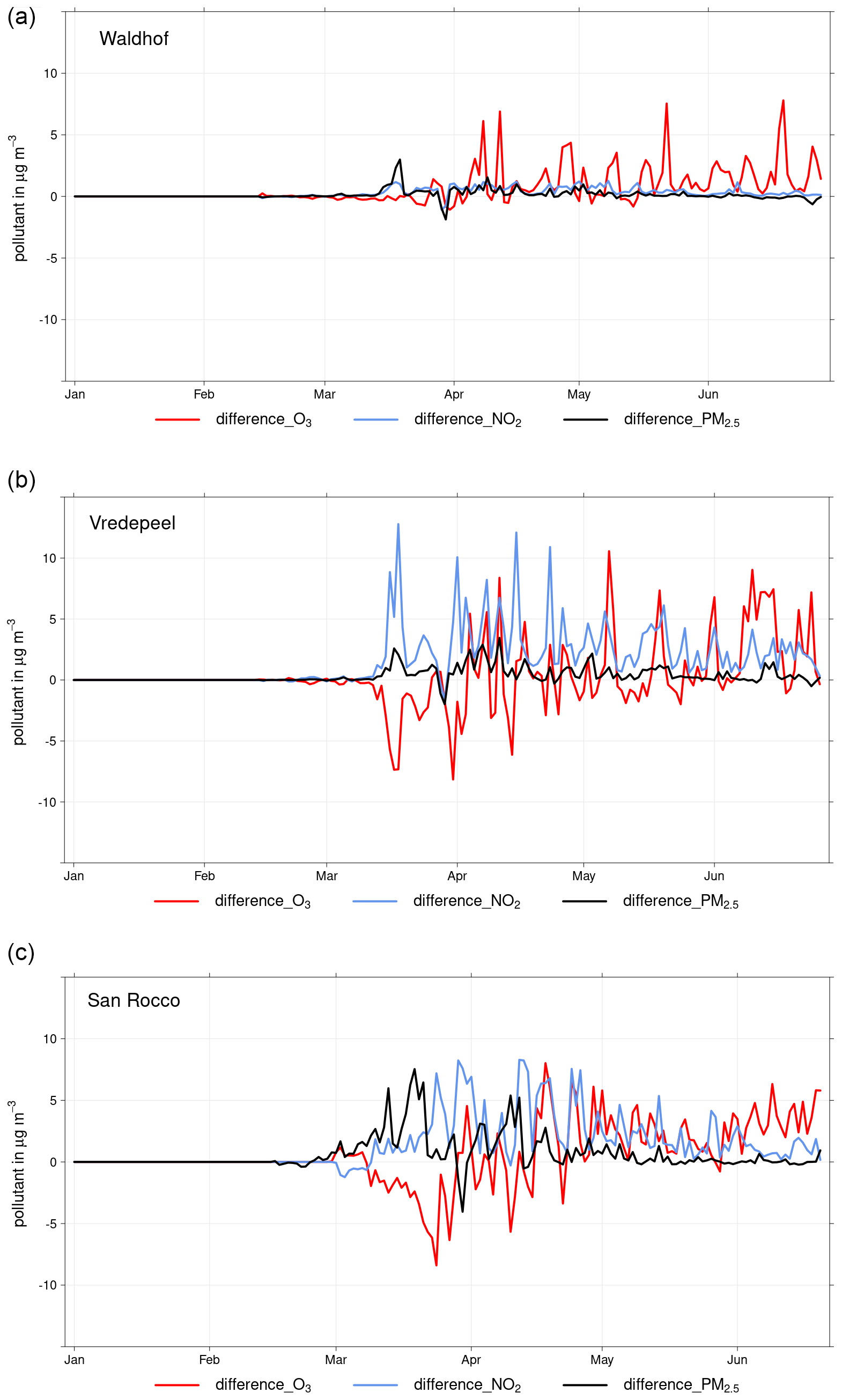
Figure 14Temporal development of the differences in the simulated concentrations of O3 (red), NO2 (blue) and PM2.5 (black) in Waldhof (a), Vredepeel (b) and San Rocco (c) between 1 January and 30 June 2020.
O3 shows higher values despite the emission reductions until the middle of April at Vredepeel and San Rocco. This is because these stations are in VOC-limited areas at that time, where NOx emission reductions lead to decreased O3 titration. This pattern changes towards the end of April, and in the following O3 is decreased on most of the days at all stations as a consequence of lower NOx emissions. This effect remains variable at Vredepeel, a station close to the region with highest NOx emissions in Europe. At Waldhof, O3 reductions are observed between the beginning of April and the end of June. On average, between 16 March and 30 June, O3 is only decreased by 0.6 µg m−3 (< 1 %) at Vredepeel. At Waldhof and San Rocco, the reductions are 1.2 µg m−3 (1.6 %) and 1.5 µg m−3 (1.9 %), respectively.
5.2 Impact of meteorological conditions
For investigating the effects of the exceptional meteorological situation on the concentration reductions in March and April 2020, additional CMAQ model simulations were performed. Meteorological data simulated with COSMO-CLM for the first 6 months in 2016 and 2018 were used as input data, together with the 2020 emissions for both the COV and the noCOV case. Biogenic emissions were also kept the same for the 2016 and 2018 runs in order to investigate effects of meteorological conditions only. These additional years were selected to cover a span of weather situations during the lockdown phase. The selected years were different but do not represent in any sense an extreme situation. They were chosen from the time span 2015 to 2019, since for these years model data generated using the same advanced model settings (model version and reanalysis data) are available. The results show the concentration and the changes caused by the lockdown measures as they would have happened under different meteorological conditions.
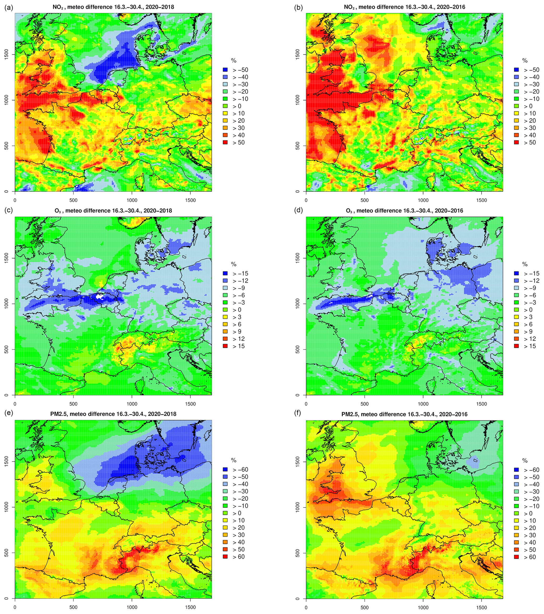
Figure 15Relative concentration changes due to meteorological conditions in central Europe between 16 March and 30 April simulated with CMAQ for NO2 (a, b), O3 (c, d) and PM2.5 (e, f): the changes are represented as relative numbers for 2020 compared to 2018 (a, c, e) and 2016 (b, d, f). Positive values denote higher concentrations in 2020 relative to the previous year. Be aware of the different scales for each pollutant.
Figure 15, top, shows the NO2 concentration changes for 2020 relative to 2018 and 2016 caused by meteorological conditions, only, for the period between 16 March and 30 April. No emission changes because of the lockdown were assumed for this investigation. Meteorological conditions in 2020 caused between 20 % and more than 30 % lower NO2 concentrations in large areas of the north-eastern model domain (the Netherlands, northern Germany, Denmark and southern Sweden) compared to 2018, even without any lockdown measures. On the other hand, in the western UK, Belgium, northern France and the Czech Republic, meteorological conditions led to 20 % to more than 30 % higher NO2 concentrations. The picture is similar when compared to 2016, in particular in the western part of the model domain, but the area with lower NO2 concentrations in 2020 compared to 2016 does not include the North Sea and Denmark.
Average ozone concentrations between 16 March and 30 April 2020 were relatively low in almost all of central Europe when compared to a situation with meteorological conditions as in 2018 and 2016 (see Fig. 15, middle). Differences are on the order of 10 %–15 % in the northern part of the model domain and between 2 % and 6 % in the southern part. Only in few spots in northern Italy and southern Switzerland, the meteorological situation in 2020 favoured ozone formation compared to 2016 and 2018.
The picture is more mixed for PM2.5, with considerably lower concentrations in 2020 compared to 2016 and 2018, particularly in northern Germany and Poland, i.e. in the north-eastern part of the domain (Fig. 15, bottom). Relative differences reach more than 50 % between 2020 and 2018 in the German Bight. Compared to 2018, PM2.5 concentrations were also low in the western UK in 2020. In almost all of France and in northern Italy, PM2.5 concentrations were relatively high in 2020 compared to 2016 and 2018, and differences again reach more than 50 % but with opposite sign.
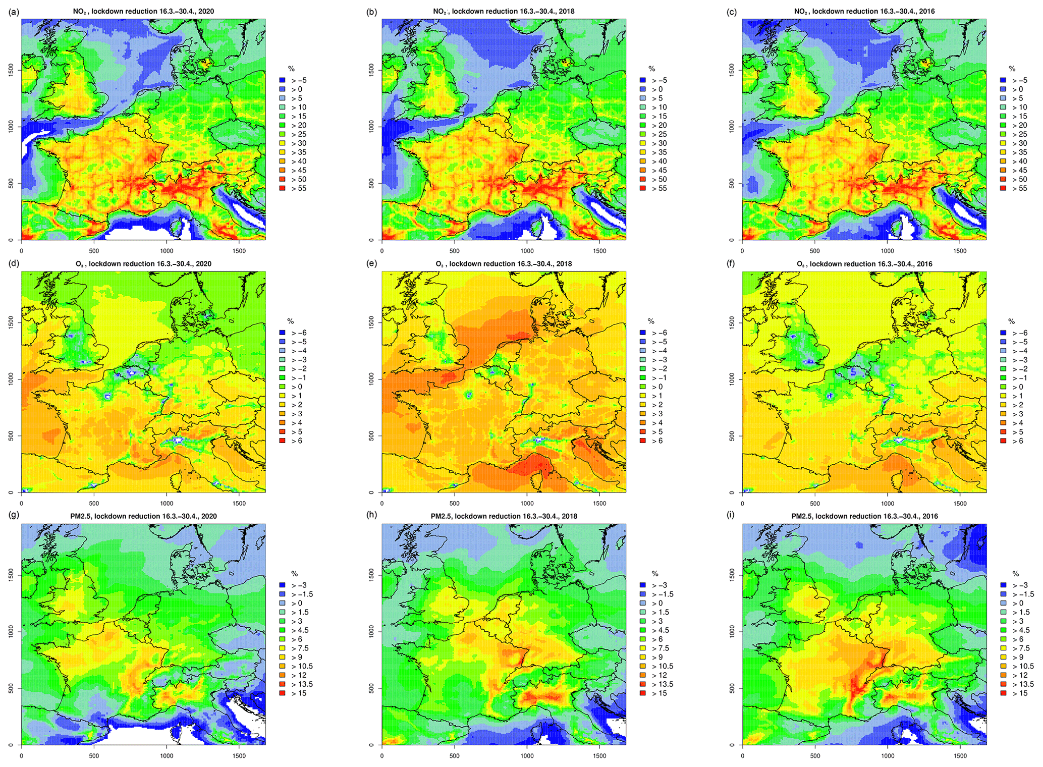
Figure 16Relative concentration reductions due to lockdown measures (noCOV – COV run) in central Europe between 16 March and 30 April simulated with CMAQ for NO2 (a–c), O3 (d–f), and PM2.5 (g–i) and three different meteorological input data sets. (a, d, g) 2020; (b, e, h) 2018; (c, f, i) 2016. Positive values denote concentration reductions caused by the lockdown emission changes. Be aware of the different scales for each pollutant.
The meteorological situation also affects the concentration changes caused by the lockdown, but this differs considerably among the pollutants. Figure 16 shows the lockdown emission reduction effects on the average concentrations for the main lockdown period from 16 March to 30 April. In most parts of central Europe the variation for NO2 is rather small (plus/minus approx. 5 %). For ozone, on the other hand, effects of the lockdown are quite different among the three selected meteorological years. For 2020 meteorological conditions, relatively large areas in northern central Europe show a slight increase in ozone (green and blue areas in Fig. 16, middle row). These areas would have been smaller with 2016 meteorological conditions and limited to the most densely populated areas for 2018 meteorological conditions. Lockdown effects on PM2.5 would have been more significant under meteorological conditions of the years 2016 and 2018 in almost the entire model domain (Fig. 16, bottom row). Particularly in northern Italy and south-eastern France, changes in PM2.5 caused by the lockdown could be more than 10 %, a value that was rarely reached during the real lockdown in 2020.
6.1 Emission estimates
Emissions for 2020 were estimated based on data for 2016 and extrapolation factors that resemble the temporal development of total sectoral emissions during 3 years before 2016. This method leads to emission corrections that are typically on the order of 10 % but may be up to 40 %. This method bears some uncertainties; however, in countries that have a high share of the total emissions in central Europe, emission trends were rather stable during the last 20 years. Good agreement between observed and modelled concentrations during the weeks before the lockdown gives confidence in the method.
Estimates for lockdown emission reductions also include several sources of uncertainty. Reduction of NOx emissions from traffic has the largest share of the emission reductions. In this approach, the LAFs applied are based on Google mobility data that resemble all traffic activities, regardless of their real emissions. That is, no distinction between trucks and small private cars is made, and it seems likely that traffic related to transporting goods was less reduced than private and commuter traffic. Therefore, emission reductions in traffic might be overestimated. On the other hand, possible emission increases for residential heating that are related to more people working from home were considered to be small and neglected here. Small changes in other sectors like off-road machinery that might have taken place were not considered either.
The cubic spline interpolation, applied to derive daily LAFs from monthly statistical data, enables us to represent the mean of each month correctly while giving an assumption on the daily values with a rather smooth curve. This assumption does not necessarily represent the real daily conditions as extrema in the interpolation always occur at the start or in the middle of the month, which might not be the case in reality. However, it is an improvement compared to using monthly averages for each day of the month, as in this case extreme jumps can occur at the transition to the next month that authors assume to be more unrealistic. In addition it might resemble the rapid emission reductions in the middle of March better than a monthly value.
Similar approaches to calculate lockdown adjustment factors were followed by Doumbia et al. (2021) and Guevara et al. (2021). Both estimate that decreases in NOx emissions in central Europe taking all sectors together were around 30 % in April 2020, which is in very good agreement with the numbers that were derived in this study. This study focuses on Europe and calculates LAFs for each country in a detailed way based on the same data source for each sector. Doumbia et al. (2021) use information from other sources than here (e.g. for aviation, shipping and industry), which are partly less well resolved in time; however, they provide adjustment factors for the entire world. Also emissions from residential areas were treated differently. While Doumbia et al. (2021) see an emission increase, they remained unchanged in this study. The reasoning behind this is that the heating demand is most likely not significantly modified when more people stay at home compared to the case when they go to work. This assumption is in agreement with earlier estimates by Le Quéré et al. (2020), who calculated only small emission increases in the residential sector. Compared to Guevara et al. (2021), the time period considered in this study is longer and reaches until the end of June 2020.
6.2 CTM results
Chemistry transport model (CTM) simulations are always connected with uncertainties, stemming from unknown or incorrectly represented processes or input data. The former includes chemical reactions, transport, and deposition processes, and the latter includes emission data and meteorological fields. Nevertheless, the model is able to reproduce observed concentration levels and their spatiotemporal variation. The agreement between modelled and observed concentrations (see Sect. 4.3) is in a range that is typical for regional CTMs (see e.g. Solazzo et al., 2012). The deviations from the observed values can be interpreted as relative uncertainties in the modelled lockdown effects. During the lockdown between March and June, deviations between modelled and observed concentrations are often higher than the changes caused by the lockdown. Therefore, the results cannot be used to judge how accurate the estimated emission reductions are. It should be noted also that the simulations for 2016 and 2018 do not resemble the real situation during these years, because all emissions and chemical boundary conditions were for 2020.
6.2.1 NO2 concentrations
During the 6 weeks of the most stringent lockdown measures in central Europe (16 March to 30 April), emission reductions caused NO2 concentration reductions between 15 % and more than 50 %. This is in good agreement with other studies (Velders et al., 2021; Menut et al., 2020; Gaubert et al., 2021) and also close to what was estimated from satellite observations. Bauwens et al. (2020) report columnar NO2 reductions of approx. 20 % around Hamburg, Frankfurt and Brussels; 28 % for the area around Paris; and 33 %–38 % for northern Italy. These reductions are almost independent of the meteorological situation, as can be seen in Fig. 16 (top row). Differences in modelled NO2 concentrations between 2020 and 2016 or 2018 show variations of more than 30 %, but they are fluctuating in both directions on small spatial scales (see Fig. 15, top row). Larger areas with systematic differences are mainly found over sea and in areas with relatively low average concentrations, like in the western UK. It can be concluded that the NO2 concentration reductions during the lockdown were dominated by the emission reductions and not very much by the meteorological situation. This is in agreement with the fact that NO2 concentrations are spatially closely connected to the emission sources. NO2 is quickly formed from NO after the latter was emitted into the atmosphere. It will then react further to form O3 at daytime. Compared to O3 and secondary PM, NO2 is a rather short-lived gas with high spatial gradients and a clear annual cycle. However, as the situation in February 2020 shows, very unusual meteorological conditions can also cause large deviations from expected concentrations.
6.2.2 O3 concentrations
Ozone concentrations depend more strongly on weather conditions and on emissions of other precursors like VOCs. Therefore, meteorological variations from year to year might have a much stronger influence on average concentrations than the emission reductions during the lockdown. The 6-week-average ozone concentrations vary by ±15 % between 2020 and 2016 or 2018 (Fig. 15, middle row), while the lockdown effects are mostly in the range of ±5 % (Fig. 16, middle row), except in densely populated areas. Weather conditions between 16 March and 30 April 2020 favoured relatively lower ozone concentrations in most parts of central Europe when compared to 2016 and 2018. In the simulations, only areas in the western Alpine region show higher ozone in 2020 (Fig. 15, middle row). First of all, this is surprising because 2020 was comparably sunny and dry, which should favour ozone formation. The latter was also stated by Deroubaix et al. (2021) and Gaubert et al. (2021) in their studies about the COVID19 lockdown effects on air quality. However, advection of relatively clean air from Scandinavia into the north-eastern part of the model domain led to lower ozone concentrations particularly in the second half of April. A comparison of the meteorological effects on NO2 and O3 in Fig. 15 also shows that NO2 was relatively high and O3 relatively low in 2020 in the English Channel, in the south-western UK and Belgium. The high-pressure situation with relatively low wind speeds in 2020 resulted in efficient ozone destruction at night in areas with high NO emissions.
Lockdown effects on ozone might differ in sign under different meteorological conditions, as can be seen in Fig. 16. The emission reductions caused relative ozone increases in urban areas and throughout the northern part of the model domain, because these areas are VOC-limited regions. This was also reported by Menut et al. (2020) and Mertens et al. (2021). The effect is most pronounced in the second half of March and then decreases over time when VOC emissions, in particular from natural sources, increase (Fig. A7). In northern central Europe the small effects on ozone are connected with advection of clean air from the north-east. For most parts of central Europe, O3 concentrations were decreased by lockdown measures. About 2 %–4 % O3 concentration reductions in most parts of central Europe could have been expected with 2018 meteorological fields, when solar radiation was lower but more southerly winds prevailed in northern central Europe. On the other hand, with 2016 meteorological conditions ozone changes would show similar patterns to 2020. Ozone chemistry depends on radiation, precipitation, atmospheric mixing and the availability of precursors in a complex way. The response of ozone concentrations to emission changes is therefore not straightforward to predict. Also long-range transport, which was neglected here, may play role (see also Deroubaix et al., 2021, and Mertens et al., 2021).
6.2.3 PM2.5 concentrations
PM2.5 is another secondary pollutant that depends strongly on weather conditions, but emission reductions will primarily lead to concentration reductions (see Figs. 13 and 14). However, the strength of this effect might also vary considerably with meteorological conditions. Figure 15 (bottom row) shows that the main lockdown period in 2020 was favourable for PM2.5 formation in most parts of central Europe, with often 20 % to 50 % higher PM2.5 concentrations compared to other meteorological situations. An exception is the north-eastern part of the model domain, where the meteorological situation in 2020 led to much lower PM2.5 concentrations compared to 2018 (more than 50 % lower) and 2016 (20 %–40 % lower). Similar to the situation for ozone, this is connected to the easterly and north-easterly winds and the advection of clean air. Consequently, lockdown emission reductions had only very minor effects on PM2.5 concentrations in 2020 in southern Sweden, Denmark, Poland and northern Germany.
Among the PM2.5 components, particle-bound nitrate is reduced the most (Figs. A9–A11). Sulfate might even increase in some areas where ammonia becomes available when ammonium nitrate aerosol concentrations are reduced. Small amounts of additional ammonium sulfate can then be formed. Reduced VOC emissions are likely to also cause a decrease in secondary organic aerosol (SOA) formation, as proposed by Gaubert et al. (2021). Given the uncertainties in SOA formation mechanisms in regional CTMs (Bessagnet et al., 2016), lockdown effects on SOA were not investigated in this study.
Higher PM2.5 reductions would have been observed in most parts of Europe with 2016 and 2018 meteorological conditions. This can be interpreted in such a way that the main lockdown period in 2020 was favourable for PM2.5 formation in large parts of Europe, leading to smaller relative PM2.5 concentration reductions, given that the emission changes are the same.
In summary, it can be said that the effects of lockdown emission reductions depend strongly on the meteorological situation and that concentration changes because of weather conditions might be stronger than those of large emission changes during a 6-week period in spring. However, this mainly holds for the secondary pollutants O3 and PM2.5, while the effects on NO2 concentrations are less pronounced. In particular, changes in O3 concentrations are difficult to predict because of the complex emission–chemistry–meteorology interactions.
Lockdown emission reductions in spring 2020 in central Europe were significant, in particular those in traffic. Other sectors, like shipping, might be of regional importance, but emission changes for this sector are less certain. Aviation shows the largest relative reduction among the emission sectors considered; however, the contribution to the total emission reductions is small because of its low share in total NOx emissions. Consequently, strongest lockdown emission reductions are seen for cities. The period with largely reduced emissions was limited to a few weeks, and emissions increased again towards the middle of 2020.
In absolute numbers, concentration reductions were strongest for NO2 in cities and for larger areas in the Po Valley with more than 6 µg m−3 for a 2-week average in the second half of March. Northern Italy also showed the strongest relative decline with more than 50 %. Rural areas in Germany, Poland and the Czech Republic showed the lowest reductions between 10 % and 20 %.
Ozone concentrations were often reduced but not in cities and not in northern Europe between the middle of March and the beginning of April. This can be explained by reduced titration in cities (NO–O3 reactions that destroy ozone) during the first phase of the lockdown, when NO emissions were lowest. The O3 concentration changes were around ±5 %, which is much less than the NO2 changes. The impacts of meteorological conditions can be much larger, and the temporary O3 increase in north-eastern Europe in March would not have taken place under meteorological conditions as they were present in the years 2016 and 2018.
PM2.5 concentrations were also decreased because of the lockdown emission reductions, but the magnitude was much smaller than for NO2, only between 2 % and 10 %. Particle-bound nitrate contributes most to this effect. Again, concentration changes can be much larger due to meteorological conditions. The reductions in 2020 were relatively lower compared to the effects with 2016 and 2018 meteorological conditions.
Because the meteorological effects on concentrations of O3 and PM2.5 are larger than the lockdown emission reduction effects, it is difficult to judge or even quantify emission reduction effects by observations and comparison with previous years only. For NO2, this is different, but in exceptional situations, like in February 2020, NO2 can also be strongly influenced by meteorological conditions and lead to lower concentrations than in March during lockdown conditions.
Meteorological and chemistry transport models need to be applied to investigate the effects of emission reductions and separate them from meteorological effects. Although these models have deficiencies and systematic errors, e.g. underestimation of NO2 and PM2.5 concentrations, the impacts of emission changes caused by the lockdown can be quantified. The model accuracy is not sufficient to judge the correctness of the emission reduction estimates; however, the calculated NO2 reductions agree well with estimations from ground-based and satellite observations for central Europe.
The emission reductions for several weeks during the first COVID-19 lockdown in Europe were the largest since decades. They can be seen as a huge test for emission reductions that could be achieved with significantly reduced car traffic and air traffic. The reductions resulted in much lower NO2 concentrations, particularly in cities, but the effects on secondary pollutants like ozone and PM2.5 were limited and are hard to predict. The latter holds particularly for ozone that might even increase in some areas when traffic emissions are decreased. Systematic changes in prevailing weather situations that might appear due to climate change could mask effects of emission reductions on secondary pollutants. The relatively short duration of strong lockdown measures also results in limited effects on annual average NO2 concentrations. Depending on location, only between 3 % and 15 % lower values could be reached.
A1 Emission data
Table A1Overview of available emission reduction information for countries in the investigated domain during the lockdown applied in this study.
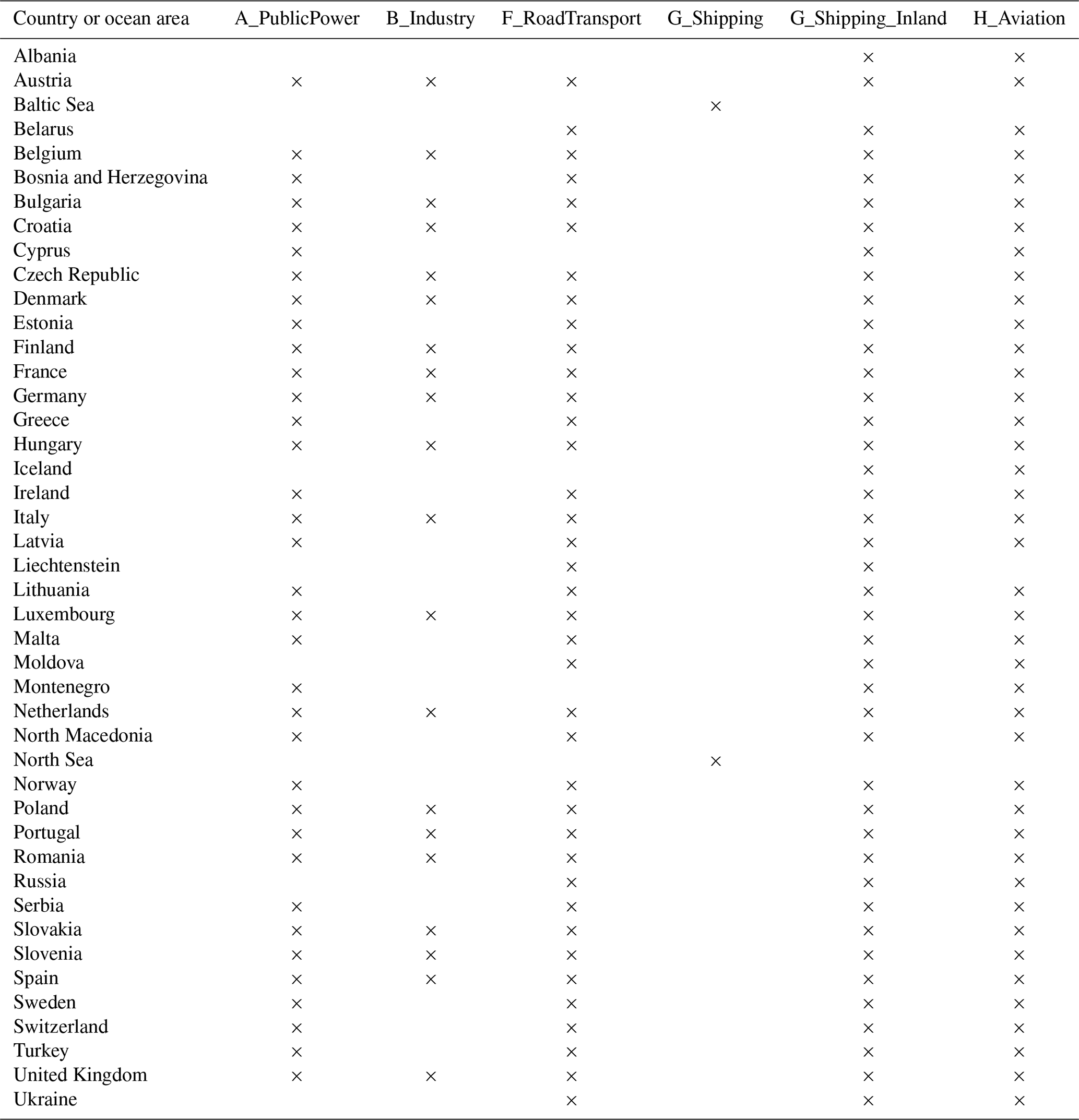
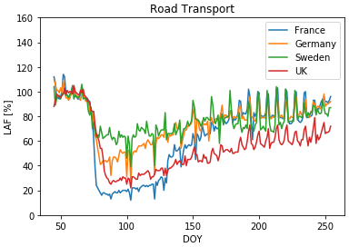
Figure A1Daily values for lockdown adjustment factors (in %) for the sector F_RoadTransport based on transit data from the Google mobility reports.
A2 Meteorological situation
Table A2GWL classification for the period 1 February–31 May 2020.
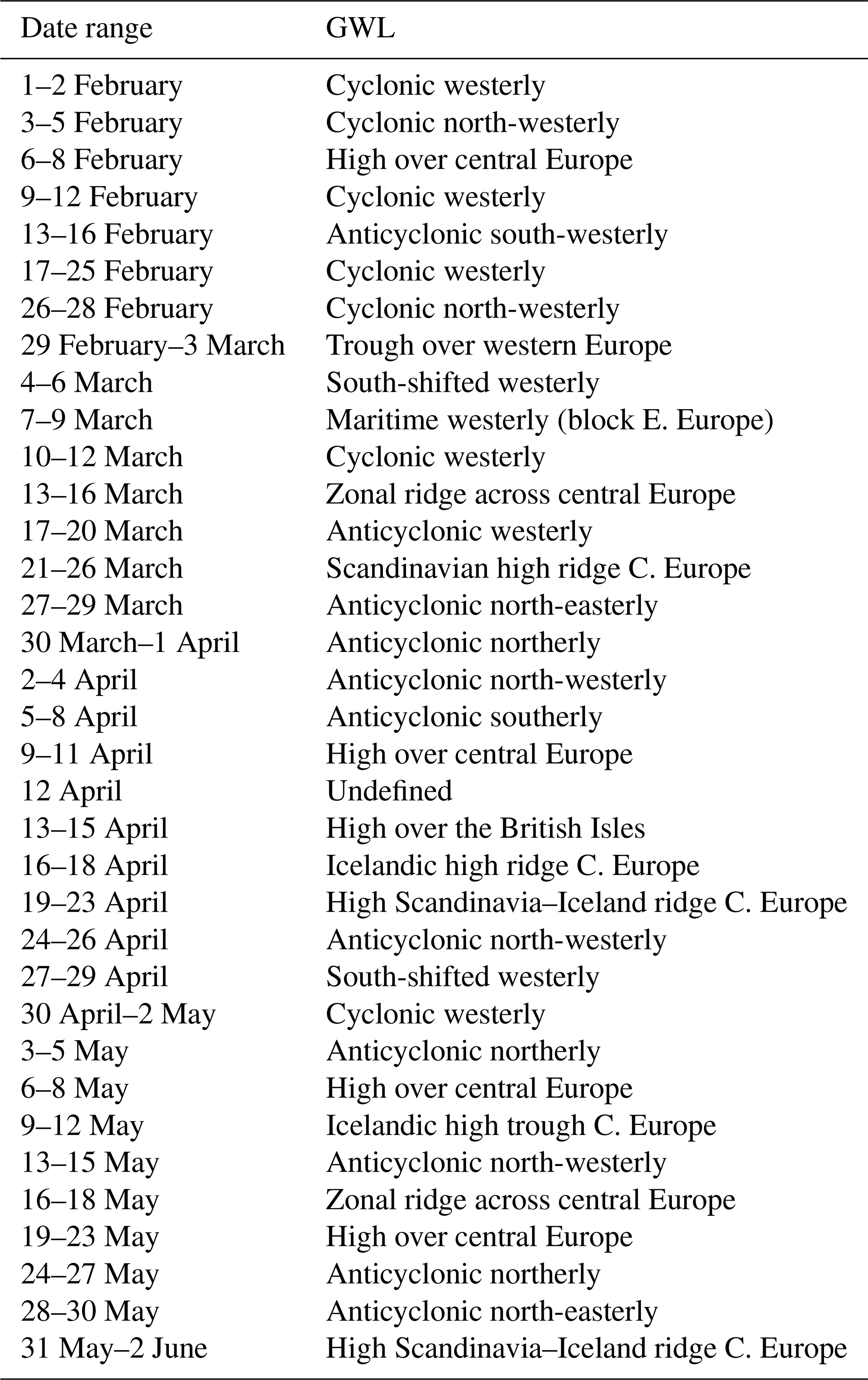
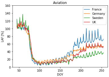
Figure A2Daily values for lockdown adjustment factors (in %) for the sector H_Aviation based on Eurocontrol data.

Figure A3Time series of the monthly accumulated precipitation and mean solar irradiance between 10:00 and 14:00 UTC at the Wettermast Hamburg for February from 1997–2020.
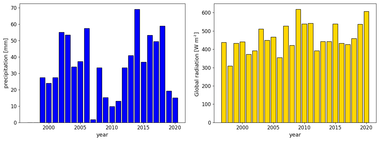
Figure A4Time series of the monthly accumulated precipitation and mean solar irradiance between 10:00 and 14:00 UTC at the Wettermast Hamburg for April from 1997–2020.
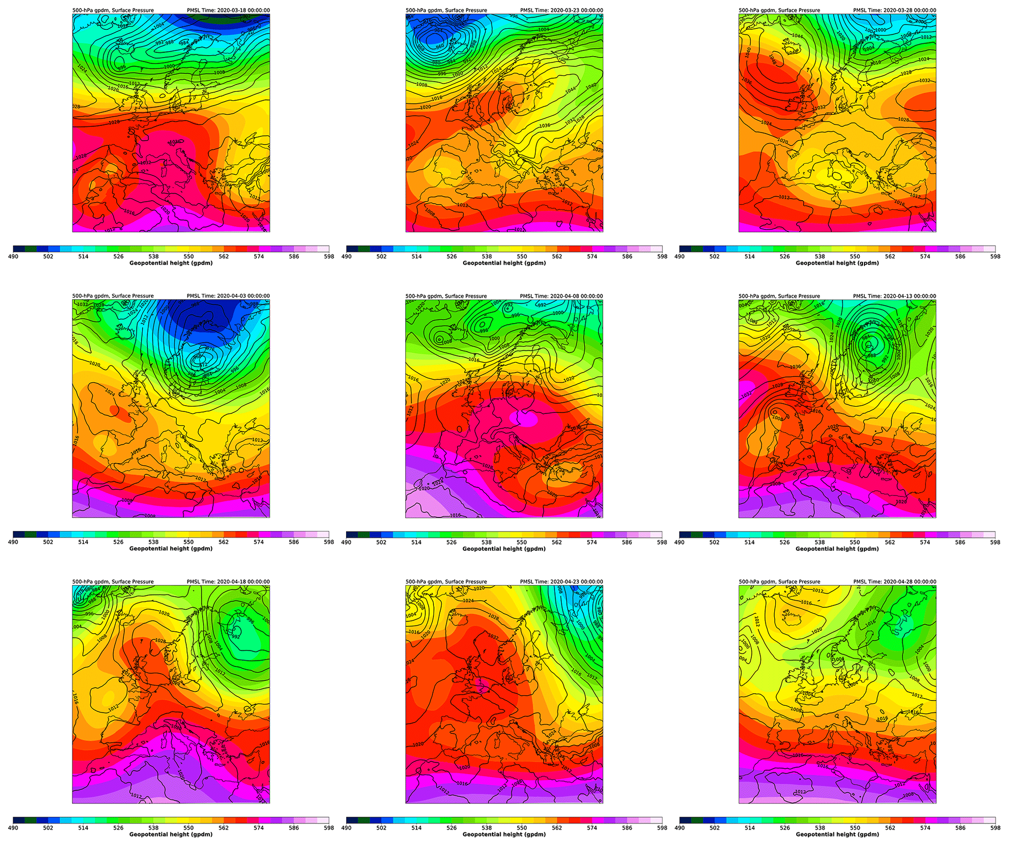
Figure A5500 hPa geopotential heights (in gpdm) and surface pressure (in hPa) for 4 d time segments in March and April 2020 according to the COSMO simulations. The geopotential heights are averaged over 4 d, and displayed surface pressure distributions are representative snapshots within those time segments.
A3 COVID-19 lockdown effects
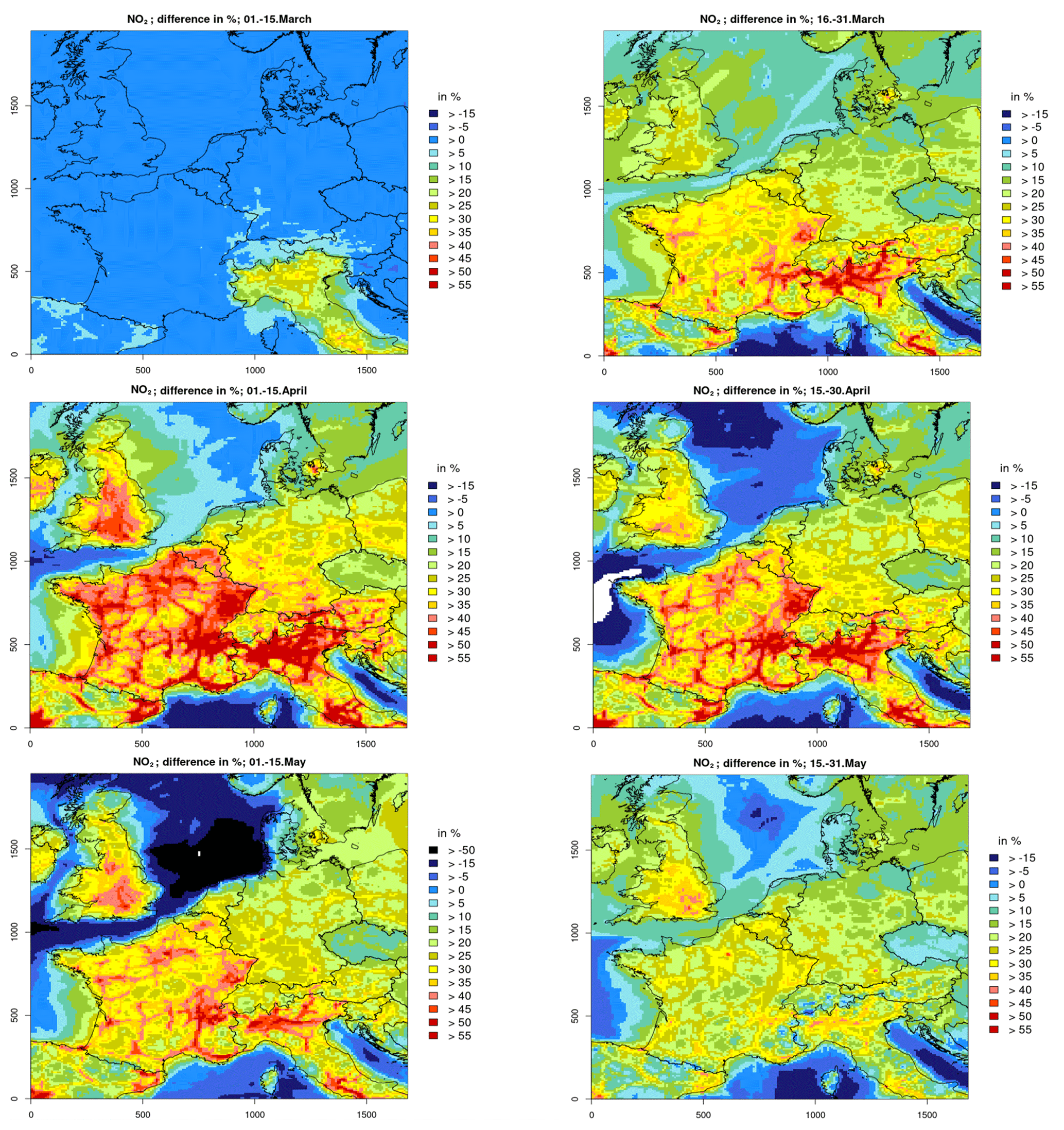
Figure A6CMAQ results for relative NO2 concentration reductions due to lockdown measures (noCOV – COV run) in central Europe between 1 March and 31 May 2020 in half-monthly intervals; positive values denote reductions.

Figure A7CMAQ results for relative O3 concentration reductions due to lockdown measures (noCOV – COV run) in central Europe between 1 March and 31 May 2020 in half-monthly intervals; positive values denote reductions.
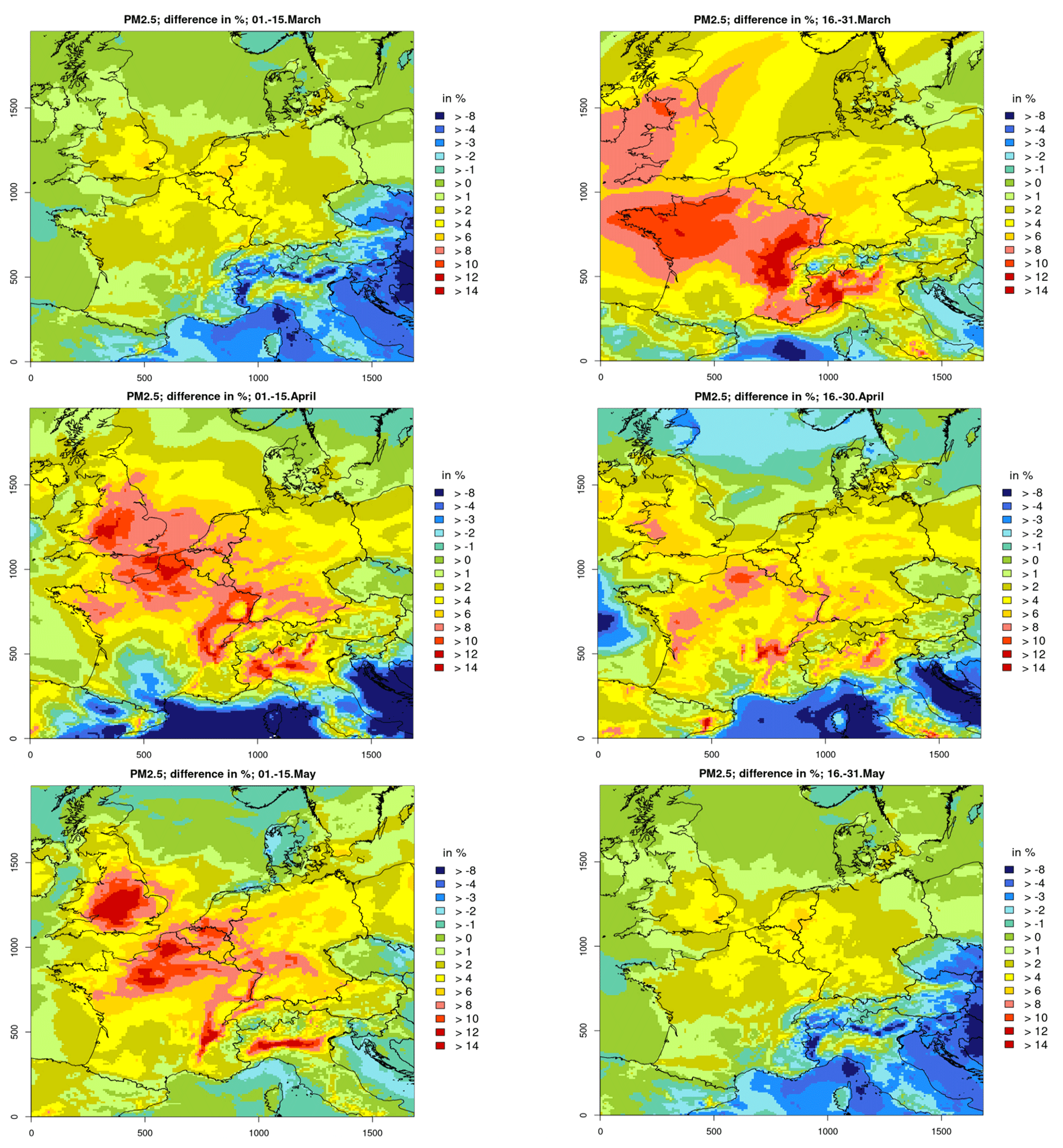
Figure A8CMAQ results for relative PM2.5 concentration reductions due to lockdown measures (noCOV – COV run) in central Europe between 1 March and 31 May 2020 in half-monthly intervals; positive values denote reductions.
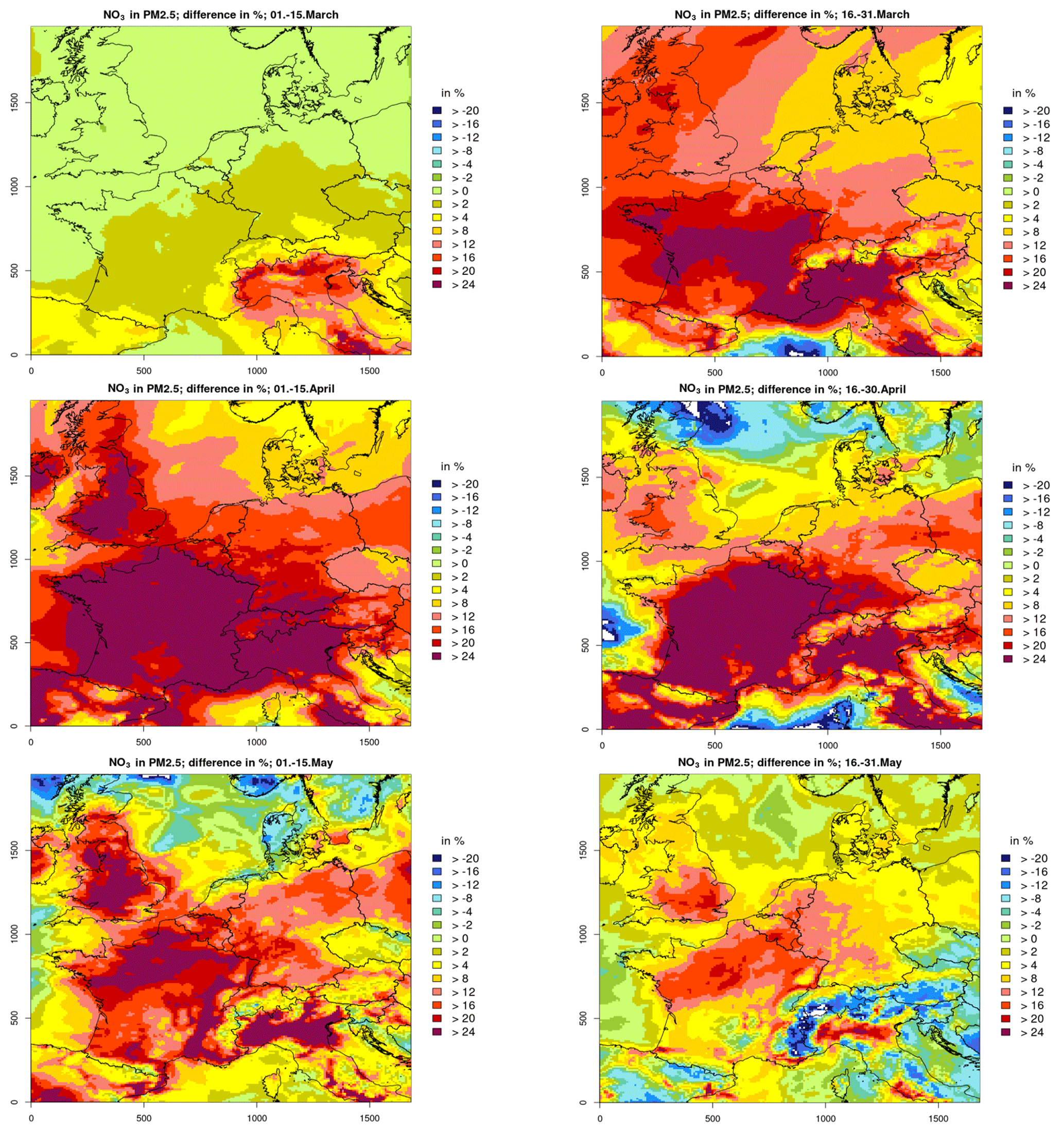
Figure A9CMAQ results for relative particulate nitrate (NO) concentration reductions due to lockdown measures (noCOV – COV run) in central Europe between 1 March and 31 May 2020 in half-monthly intervals; positive values denote reductions.
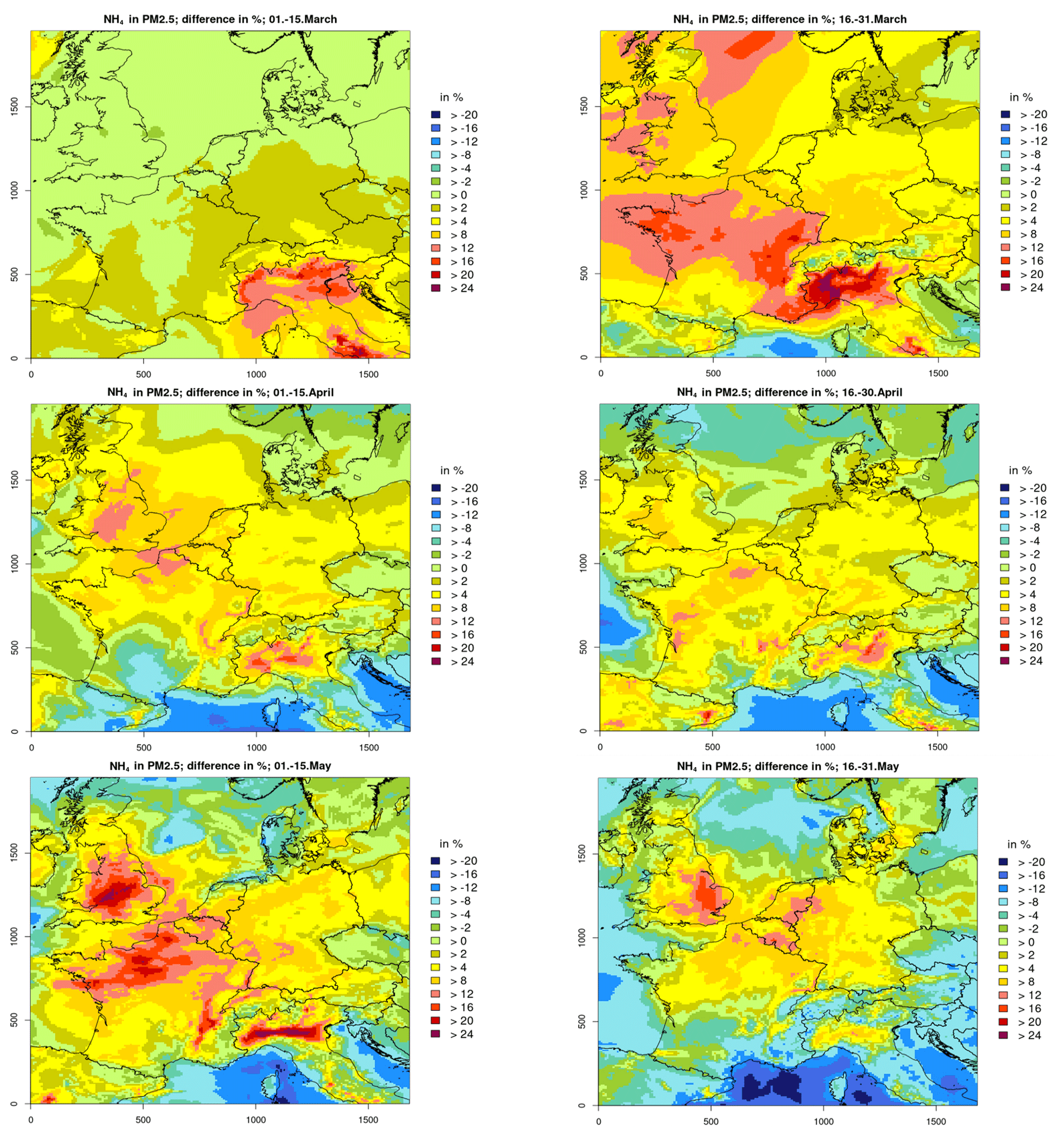
Figure A10CMAQ results for relative particulate ammonium (NH) concentration reductions due to lockdown measures (noCOV – COV run) in central Europe between 1 March and 31 May 2020 in half-monthly intervals; positive values denote reductions.
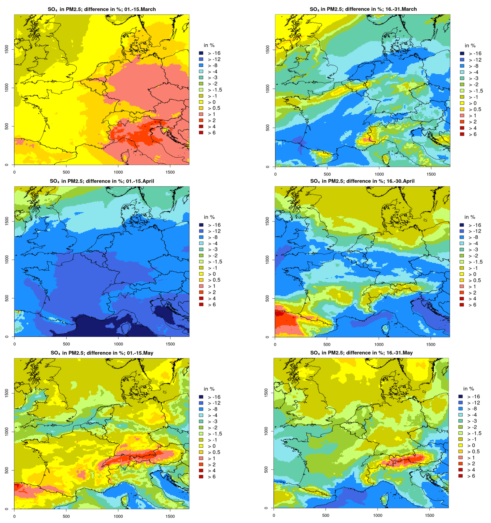
Figure A11CMAQ results for relative particulate sulfate (SO) concentration reductions due to lockdown measures (noCOV – COV run) in central Europe between 1 March and 31 May 2020 in half-monthly intervals; positive values denote reductions.

Figure A12CMAQ results for concentrations of PM2.5 and its components nitrate, ammonium and sulfate in central Europe between 16 and 31 March 2020.
A4 Meteorological differences for 2020 versus 2016 and 2018
In 2020 the geopotential height at 500 hPa over the British Isles and the North Sea was significantly higher compared to that in 2016, especially from 1 April onward. This resulted in a constellation which favours blocking in 2020. Near-surface high-pressure systems were amplified, and more persistent and weak wind conditions and a more continental flow dominate. In 2016 stronger winds of Atlantic origin occasionally were observed. In 2020 precipitation was considerably lower compared to 2016. In most parts of the study region solar radiation was clearly higher in 2020, especially over central Europe up to the British Isles.
Much of what has been said concerning the blocking condition in 2020 holds as well when compared to 2018. The year 2020 was also much drier, and incoming solar radiation was more intense. In 2018, winds had a more easterly to south-easterly component. The spatial and temporal distribution and the absolute values of the meteorological parameters were slightly different in 2018 compared to 2016 (see Figs. A13–A15), so this year became an additional choice for the evaluation of meteorological influences.
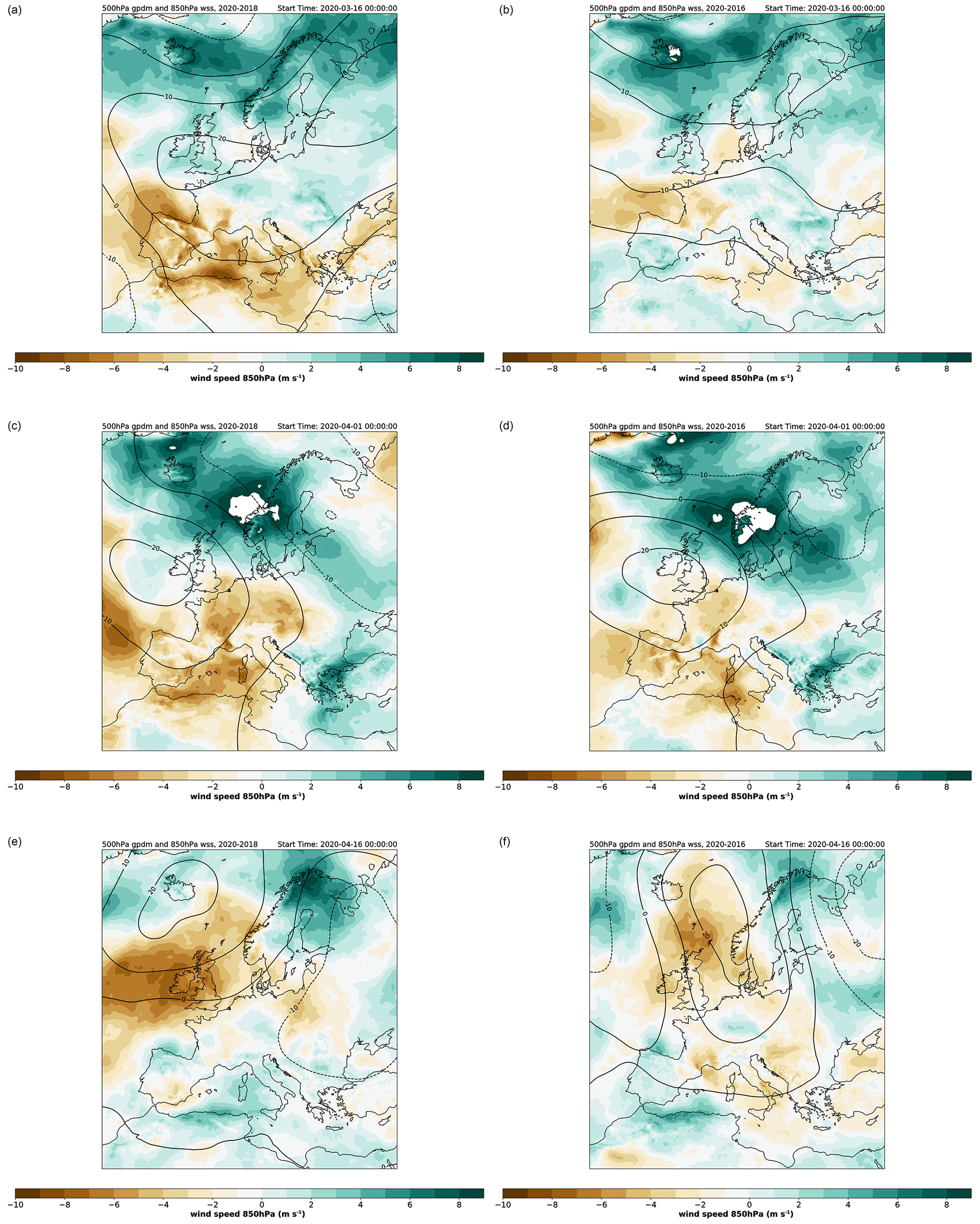
Figure A13Geopotential height at 500 hPa (in gpdm, isolines) and wind speed at 850 hPa (in m s−1, colour code): differences between 2020 and 2018 (a, c, e) and between 2020 and 2016 (b, d, f) for the half-month periods 16–31 March (a, b), 1–15 April (c, d) and 16–30 April (e, f).
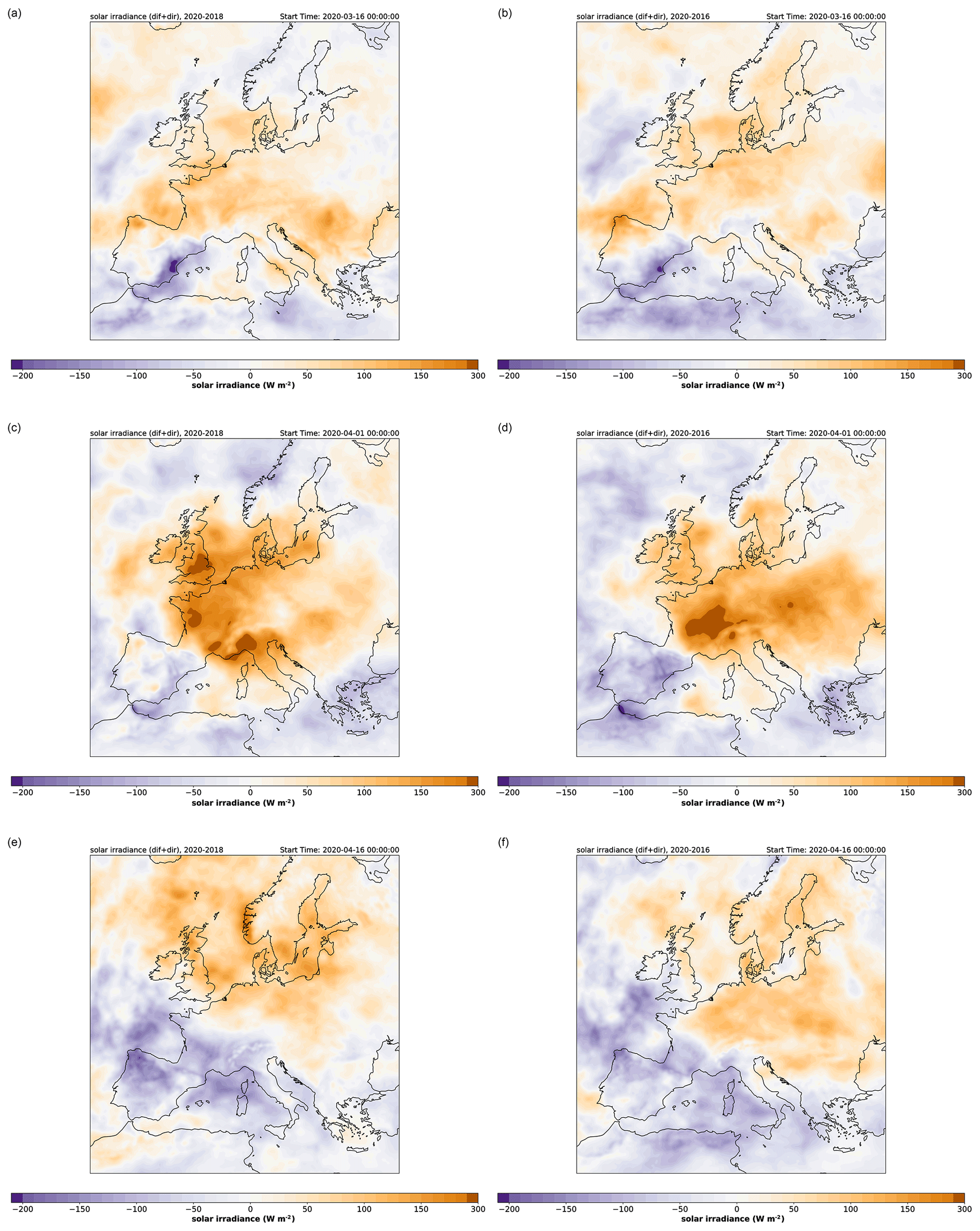
Figure A14Solar irradiance (in W m−2, colour code): differences between 2020 and 2018 (a, c, e) and between 2020 and 2016 (b, d, f) for the half-month periods 16–31 March (a, b), 1–15 April (c, d) and 16–30 April (e, f).
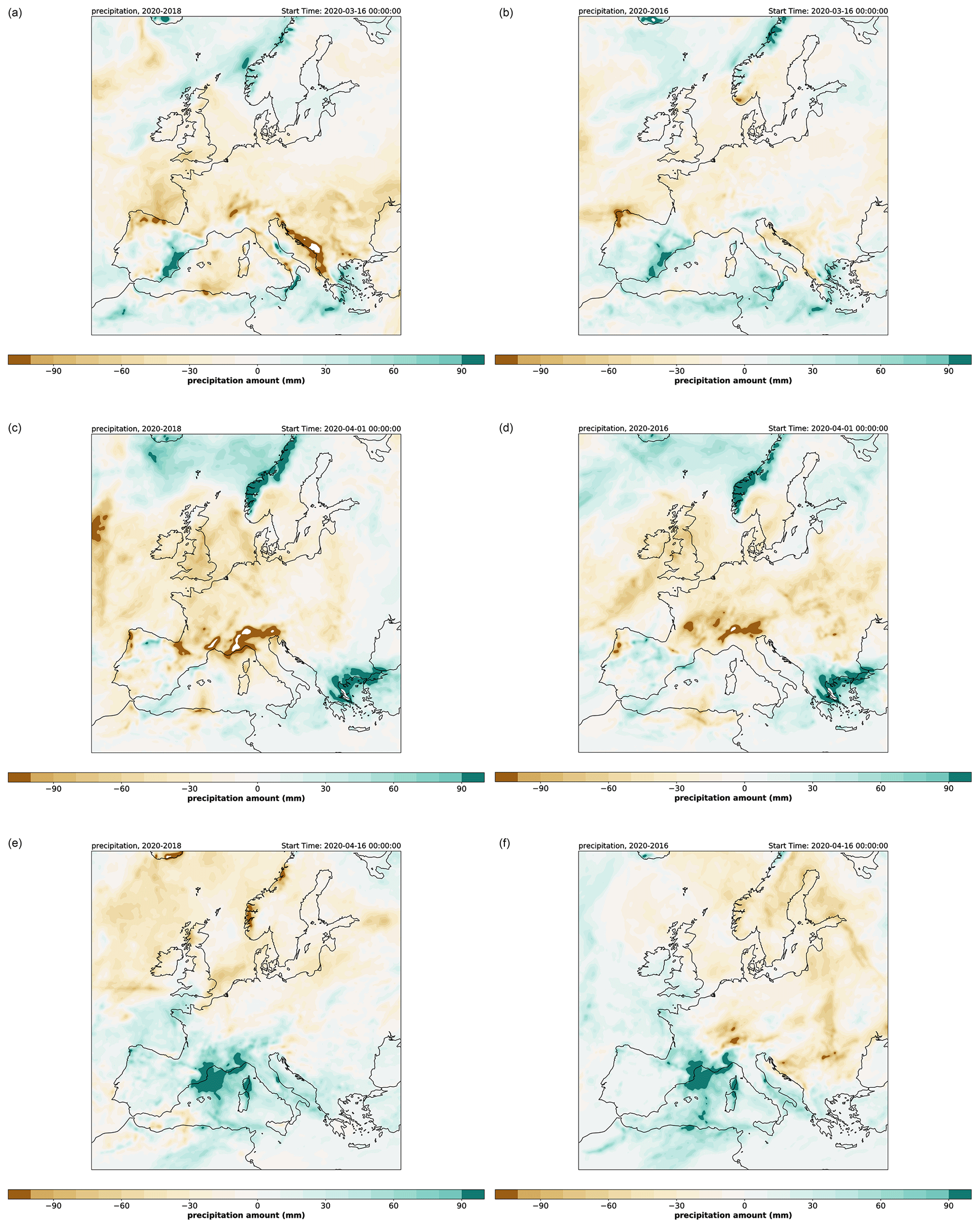
Figure A15Accumulated precipitation (in mm, colour code): differences between 2020 and 2018 (a, c, e) and between 2020 and 2016 (b, d, f) for the half-month periods 16–31 March (a, b), 1–15 April (c, d) and 16–30 April (e, f).
The CMAQ code is available through the US EPA at https://github.com/USEPA/CMAQ (last access: 16 September 2021). CMAQ version 5.2, which was used here, is available at https://doi.org/10.5281/zenodo.1167892 (US EPA Office of Research and Development, 2017).
The COSMO-CLM model is documented at https://wiki.coast.hereon.de/clmcom (last access: 16 September 2021, COSMO-CLM Community, 2021). The model code is available for registered users of the CLM community.
Lockdown adjustment factors (LAFs) and projection factors (PFs), as well as CMAQ model results, are available upon request.
VM developed the idea, designed and supervised the study, evaluated part of the model results, prepared the manuscript, and wrote most of the text. MQ co-designed the study, wrote most of the text about the meteorological situation and provided interpretations of the meteorology–chemistry interactions. JAA helped in designing the study, performed CMAQ model runs and provided code for the emission data preparation. RB developed the lockdown adjustment factors, extrapolated emission data and wrote the section about the emission data. LF performed CMAQ model runs, evaluated CMAQ model results and observation data, and provided most of the plots. RP performed COSMO model runs, provided information for the meteorological data interpretation, wrote the text about the COSMO setup and part of the text about the meteorological situation, and analysed COSMO model results. JF developed emission extrapolation factors and provided interpretation of the observational data. DS analysed AIS data and calculated ship emission LAFs. EML collected and analysed observational data and provided data interpretation. MOPR helped in designing the study and analysed and interpreted observational data for suburban stations. RW collected data on aviation emissions, provided LAFs for aviation and contributed to the discussion of the results.
The contact author has declared that neither they nor their co-authors have any competing interests.
Publisher’s note: Copernicus Publications remains neutral with regard to jurisdictional claims in published maps and institutional affiliations.
The Community Multiscale Air Quality Modeling System (CMAQ) is developed and maintained by the US EPA. Its use is gratefully acknowledged. Jeroen Kuenen from TNO, Department of Climate, Air and Sustainability, is acknowledged for the provision of NMVOC splits for use with the CAMS-REGAP-EU emission inventory. The data were downloaded from the Emissions of atmospheric Compounds and Compilation of Ancillary Data (ECCAD) web page (https://eccad3.sedoo.fr/, last access: 16 September 2021). Creation and maintenance of the web site is gratefully acknowledged.
We thank the weather mast group of the Meteorological Institute at the University of Hamburg, who delivered data from tower site Wettermast Hamburg.
We also thank the German Maritime and Hydrographic Agency for supporting us with AIS data taken in Bremerhaven, Hamburg and Kiel.
The article processing charges for this open-access publication were covered by the Helmholtz-Zentrum Hereon.
This paper was edited by Aurélien Dommergue and reviewed by three anonymous referees.
Amouei Torkmahalleh, M., Akhmetvaliyeva, Z., Omran, A. D., Faezeh Darvish Omran, F., Kazemitabar, M., Naseri, M., Naseri, M., Sharifi, H., Malekipirbazari, M., Kwasi Adotey, E., Gorjinezhad, S., Eghtesadi, N., Sabanov, S., Alastuey, A., de Fátima Andrade, M., Buonanno, G., Carbone, S., Cárdenas-Fuentes, D. E., Cassee, F. R., Dai, Q., Henríquez, A., Hopke, P. K., Keronen, P., Khwaja, H. A., Kim, J., Kulmala, M., Kumar, P., Kushta, J., Kuula, J., Massagué, J., Mitchell, T., Mooibroek, D., Morawska, L., Niemi, J. V., Ngagine, S. H., Norman, M., Oyama, B., Oyola, P., Öztürk, F., Petäjä, T., Querol, X., Rashidi, Y., Reyes, F., Ross-Jones, M., Salthammer, T., Savvides, C., Stabile, L., Sjöberg, K., Söderlund, K., Sunder Raman, R., Timonen, H., Umezawa, M., Viana, M., and Xie, S.: Global Air Quality and COVID-19 Pandemic: Do We Breathe Cleaner Air?, Aerosol Air Qual. Res., 21, 200567, https://doi.org/10.4209/aaqr.200567, 2021.
Baldauf, M., Seifert, A., Forstner, J., Majewski, D., Raschendorfer, M., and Reinhardt, T.: Operational Convective-Scale Numerical Weather Prediction with the COSMO Model: Description and Sensitivities, Mon. Weather Rev., 139, 3887–3905, https://doi.org/10.1175/mwr-d-10-05013.1, 2011.
Baret, F., Weiss, M., Lacaze, R., Camacho, F., Makhmara, H., Pacholcyzk, P., and Smets, B.: GEOV1: LAI and FAPAR essential climate variables and FCOVER global time series capitalizing over existing products. Part1: Principles of development and production, Remote Sens. Environ., 137, 299–309, https://doi.org/10.1016/j.rse.2012.12.027, 2013.
Bauwens, M., Compernolle, S., Stavrakou, T., Muller, J. F., van Gent, J., Eskes, H., Levelt, P. F., van der, A. R., Veefkind, J. P., Vlietinck, J., Yu, H., and Zehner, C.: Impact of coronavirus outbreak on NO2 pollution assessed using TROPOMI and OMI observations, Geophys. Res. Lett., 47, e2020GL087978, https://doi.org/10.1029/2020GL087978, 2020.
Bessagnet, B., Pirovano, G., Mircea, M., Cuvelier, C., Aulinger, A., Calori, G., Ciarelli, G., Manders, A., Stern, R., Tsyro, S., García Vivanco, M., Thunis, P., Pay, M.-T., Colette, A., Couvidat, F., Meleux, F., Rouïl, L., Ung, A., Aksoyoglu, S., Baldasano, J. M., Bieser, J., Briganti, G., Cappelletti, A., D'Isidoro, M., Finardi, S., Kranenburg, R., Silibello, C., Carnevale, C., Aas, W., Dupont, J.-C., Fagerli, H., Gonzalez, L., Menut, L., Prévôt, A. S. H., Roberts, P., and White, L.: Presentation of the EURODELTA III intercomparison exercise – evaluation of the chemistry transport models' performance on criteria pollutants and joint analysis with meteorology, Atmos. Chem. Phys., 16, 12667–12701, https://doi.org/10.5194/acp-16-12667-2016, 2016.
Bieser, J., Aulinger, A., Matthias, V., Quante, M., and Builtjes, P.: SMOKE for Europe – adaptation, modification and evaluation of a comprehensive emission model for Europe, Geosci. Model Dev., 4, 47–68, https://doi.org/10.5194/gmd-4-47-2011, 2011a.
Bieser, J., Aulinger, A., Matthias, V., Quante, M., and Denier van der Gon, H. A. C.: Vertical emission profiles for Europe based on plume rise calculations, Environ. Pollut., 159, 2935–2946, 2011b.
Bissolli, P. and Dittmann, E.: The objective weather type classification of the German Weather Service and its possibilities of application to environmental and meteorological investigations, Meteorol. Z., 10, 253–260, https://doi.org/10.1127/0941-2948/2001/0010-0253, 2001.
Brümmer, B. and Schultze, M.: Analysis of a 7-year low-level temperature inversion data set measured at the 280 m high Hamburg weather mast, Meteorol. Z., 24, 481–494, https://doi.org/10.1127/metz/2015/0669, 2015.
Byun, D. and Schere, K. L.: Review of the Governing Equations, Computational Algorithms, and Other Components of the Models-3 Community Multiscale Air Quality (CMAQ) Modeling System, Appl. Mech. Rev., 59, 51–77, 2006.
Byun, D. W. and Ching, J. K. S.: Science Algorithms of the EPA Models-3 Community Multiscale Air Quality Modeling System, Environmental Protection Agency, Washington, DC, USA, EPA600/R-99/030, 757 pp., 1999.
COSMO-CLM community: COSMO-CLM model, documentation available at: https://wiki.coast.hereon.de/clmcom, last access: 16 September 2021.
Collivignarelli, M. C., Abba, A., Caccamo, F. M., Bertanza, G., Pedrazzani, R., Baldi, M., Ricciardi, P., and Miino, M. C.: Can particulate matter be identified as the primary cause of the rapid spread of CoViD-19 in some areas of Northern Italy?, Environ. Sci. Pollut. R., 28, 33120–33132, https://doi.org/10.1007/s11356-021-12735-x, 2020.
Denier van der Gon, H. A. C., Hendriks, C., Kuenen, J., Segers, A., and Visschedijk, A.: Description of current temporal emission patterns and sensitivity of predicted AQ for temporal emission patterns, EU FP7 MACC deliverable report D_D-EMIS_1.3, TNO, Utrecht, available at: https://atmosphere.copernicus.eu/sites/default/files/2019-07/MACC_TNO_del_1_3_v2.pdf (last access: 16 September 2021), 2011.
Deroubaix, A., Brasseur, G., Gaubert, B., Labuhn, I., Menut, L., Siour, G., and Tuccella, P.: Response of surface ozone concentration to emission reduction and meteorology during the COVID-19 lockdown in Europe, Meteorol. Appl., 28, e1990, https://doi.org/10.1002/met.1990, 2021.
Doms, G. and Schättler, U.: A Description of the Nonhydrostatic Regional Model LM. Part I: Dynamics and Numerics, Deutscher Wetterdienst, Offenbach, 140 pp., available at: https://www.dwd.de/SharedDocs/downloads/EN/model_description/nwp/lm_parts/lm_docu_1_dynamics_200211_en.pdf (last access: 16 September 2021), 2002.
Doms, G., Förstner, J., Heise, E., Herzog, H.-J., Mironow, D., Raschendorfer, M., Reinhart, T., Ritter, B., Schrodin, R., Schulz, J.-P., and Vogel, G.: A Description of the Nonhydrostatic Regional COSMO Model. Part II: Physical Parameterization, Deutscher Wetterdienst, Offenbach, 161 pp., available at: http://www.cosmo-model.org/content/model/documentation/core/cosmo_physics_4.20.pdf (last access: 16 September 2021), 2011.
Doumbia, T., Granier, C., Elguindi, N., Bouarar, I., Darras, S., Brasseur, G., Gaubert, B., Liu, Y., Shi, X., Stavrakou, T., Tilmes, S., Lacey, F., Deroubaix, A., and Wang, T.: Changes in global air pollutant emissions during the COVID-19 pandemic: a dataset for atmospheric modeling, Earth Syst. Sci. Data, 13, 4191–4206, https://doi.org/10.5194/essd-13-4191-2021, 2021.
Forster, P. M., Forster, H. I., Evans, M. J., Gidden, M. J., Jones, C. D., Keller, C. A., Lamboll, R. D., Quéré, C. L., Rogelj, J., Rosen, D., Schleussner, C.-F., Richardson, T. B., Smith, C. J., and Turnock, S. T.: Current and future global climate impacts resulting from COVID-19, Nat. Clim. Change, 10, 913–919, https://doi.org/10.1038/s41558-020-0883-0, 2020.
Gaubert, B., Bouarar, I., Doumbia, T., Liu, Y., Stavrakou, T., Deroubaix, A., Darras, S., Elguindi, N., Granier, C., Lacey, F., Müller, J.-F., Shi, X., Tilmes, S., Wang, T., and Brasseur, G. P.: Global Changes in Secondary Atmospheric Pollutants During the 2020 COVID-19 Pandemic, J. Geophys. Res.-Atmos., 126, e2020JD034213, https://doi.org/10.1029/2020JD034213, 2021.
Gelaro, R., McCarty, W., Suarez, M. J., Todling, R., Molod, A., Takacs, L., Randles, C. A., Darmenov, A., Bosilovich, M. G., Reichle, R., Wargan, K., Coy, L., Cullather, R., Draper, C., Akella, S., Buchard, V., Conaty, A., da Silva, A. M., Gu, W., Kim, G. K., Koster, R., Lucchesi, R., Merkova, D., Nielsen, J. E., Partyka, G., Pawson, S., Putman, W., Rienecker, M., Schubert, S. D., Sienkiewicz, M., and Zhao, B.: The Modern-Era Retrospective Analysis for Research and Applications, Version 2 (MERRA-2), J. Climate, 30, 5419–5454, https://doi.org/10.1175/jcli-d-16-0758.1, 2017.
Gerstengarbe, F.-W. and Werner, P. C.: Katalog der Großwetterlagen Europas nach Paul Hess und Helmut Brezowski 1881–1992, Deutscher Wetterdienst, Offenbach a.M., Berichte Deutscher Wetterdienst 113, 244 pp., available at: https://www.dwd.de/DE/leistungen/pbfb_verlag_berichte/pdf_einzelbaende/113_pdf (last access: 16 September 2021), 1993.
Gkatzelis, G. I., Gilman, J. B., Brown, S. S., Eskes, H., Gomes, A. R., Lange, A. C., McDonald, B. C., Peischl, J., Petzold, A., Thompson, C. R., and Kiendler-Scharr, A.: The global impacts of COVID-19 lockdowns on urban air pollution: A critical review and recommendations, Elem. Sci. Anth., 9, 00176, https://doi.org/10.1525/elementa.2021.00176, 2021.
Goldberg, D. L., Anenberg, S. C., Griffin, D., McLinden, C. A., Lu, Z., and Streets, D. G.: Disentangling the Impact of the COVID-19 Lockdowns on Urban NO2 From Natural Variability, Geophys. Res. Lett., 47, e2020GL089269, https://doi.org/10.1029/2020GL089269, 2020.
Granier, C., Darras, S., Gon, H. D. v. d., Doubalova, J., Elguindi, N., Galle, B., Gauss, M., Guevara, M., Jalkanen, J.-P., Kuenen, J., Liousse, C., Quack, B., Simpson, D., and Sindelarova, K.: The Copernicus Atmosphere Monitoring Service global and regional emissions (April 2019 version), Copernicus Atmosphere Monitoring Service (CAMS) report, https://doi.org/10.24380/d0bn-kx16, 2019.
Guenther, A., Jiang, X., Shah, T., Huang, L., S. Kemball-Cook, and Yarwood, G.: Model of Emissions of Gases and Aerosol from Nature Version 3 (MEGAN3) for Estimating Biogenic Emissions, Air Pollution Modeling and Its Application XXVI, edited by: Mensink, C., Gong, W., and Hakami, A., Springer International Publishing, Cham, Switzerland, 187–192, 2020.
Guenther, A. B., Jiang, X., Heald, C. L., Sakulyanontvittaya, T., Duhl, T., Emmons, L. K., and Wang, X.: The Model of Emissions of Gases and Aerosols from Nature version 2.1 (MEGAN2.1): an extended and updated framework for modeling biogenic emissions, Geosci. Model Dev., 5, 1471–1492, https://doi.org/10.5194/gmd-5-1471-2012, 2012.
Guevara, M., Jorba, O., Soret, A., Petetin, H., Bowdalo, D., Serradell, K., Tena, C., Denier van der Gon, H., Kuenen, J., Peuch, V.-H., and Pérez García-Pando, C.: Time-resolved emission reductions for atmospheric chemistry modelling in Europe during the COVID-19 lockdowns, Atmos. Chem. Phys., 21, 773–797, https://doi.org/10.5194/acp-21-773-2021, 2021.
Huang, X., Ding, A., Gao, J., Zheng, B., Zhou, D., Qi, X., Tang, R., Wang, J., Ren, C., Nie, W., Chi, X., Xu, Z., Chen, L., Li, Y., Che, F., Pang, N., Wang, H., Tong, D., Qin, W., Cheng, W., Liu, W., Fu, Q., Liu, B., Chai, F., Davis, S. J., Zhang, Q., and He, K.: Enhanced secondary pollution offset reduction of primary emissions during COVID-19 lockdown in China, Natl. Sci. Rev., 8, nwaa137, https://doi.org/10.1093/nsr/nwaa137, 2020.
Inness, A., Ades, M., Agustí-Panareda, A., Barré, J., Benedictow, A., Blechschmidt, A.-M., Dominguez, J. J., Engelen, R., Eskes, H., Flemming, J., Huijnen, V., Jones, L., Kipling, Z., Massart, S., Parrington, M., Peuch, V.-H., Razinger, M., Remy, S., Schulz, M., and Suttie, M.: The CAMS reanalysis of atmospheric composition, Atmos. Chem. Phys., 19, 3515–3556, https://doi.org/10.5194/acp-19-3515-2019, 2019.
James, P. M.: An objective classification method for Hess and Brezowsky Grosswetterlagen over Europe, Theor. Appl. Climatol., 88, 17–42, https://doi.org/10.1007/s00704-006-0239-3, 2007.
Kelly, J. T., Bhave, P. V., Nolte, C. G., Shankar, U., and Foley, K. M.: Simulating emission and chemical evolution of coarse sea-salt particles in the Community Multiscale Air Quality (CMAQ) model, Geosci. Model Dev., 3, 257–273, https://doi.org/10.5194/gmd-3-257-2010, 2010.
Kroll, J. H., Heald, C. L., Cappa, C. D., Farmer, D. K., Fry, J. L., Murphy, J. G., and Steiner, A. L.: The complex chemical effects of COVID-19 shutdowns on air quality, Nat. Chem., 12, 777–779, https://doi.org/10.1038/s41557-020-0535-z, 2020.
Le Quéré, C., Jackson, R. B., Jones, M. W., Smith, A. J. P., Abernethy, S., Andrew, R. M., De-Gol, A. J., Willis, D. R., Shan, Y., Canadell, J. G., Friedlingstein, P., Creutzig, F., and Peters, G. P.: Temporary reduction in daily global CO2 emissions during the COVID-19 forced confinement, Nat. Clim. Change, 10, 647–653, https://doi.org/10.1038/s41558-020-0797-x, 2020.
Lonati, G. and Riva, F.: Regional Scale Impact of the COVID-19 Lockdown on Air Quality: Gaseous Pollutants in the Po Valley, Northern Italy, Atmosphere, 12, 264, https://doi.org/10.3390/atmos12020264, 2021.
Matthias, V., Arndt, J. A., Aulinger, A., Bieser, J., van der Gon, H. D., Kranenburg, R., Kuenen, J., Neumann, D., Pouliot, G., and Quante, M.: Modeling emissions for three-dimensional atmospheric chemistry transport models, J. Air Waste Manage., 68, 763–800, https://doi.org/10.1080/10962247.2018.1424057, 2018.
Menut, L., Bessagnet, B., Siour, G., Mailler, S., Pennel, R., and Cholakian, A.: Impact of lockdown measures to combat Covid-19 on air quality over western Europe, Sci. Total Environ., 741, 140426, https://doi.org/10.1016/j.scitotenv.2020.140426, 2020.
Mertens, M., Jöckel, P., Matthes, S., Nützel, M., Grewe, V., and Sausen, R.: COVID-19 induced lower-tropospheric ozonechanges, Environ. Res. Lett., 16, 064005, https://doi.org/10.1088/1748-9326/abf191, 2021.
Petetin, H., Bowdalo, D., Soret, A., Guevara, M., Jorba, O., Serradell, K., and Pérez García-Pando, C.: Meteorology-normalized impact of the COVID-19 lockdown upon NO2 pollution in Spain, Atmos. Chem. Phys., 20, 11119–11141, https://doi.org/10.5194/acp-20-11119-2020, 2020.
Petrik, R., Geyer, B., and Rockel, B.: On the diurnal cycle and variability of winds in the lower planetary boundary layer: evaluation of regional reanalyses and hindcasts, Tellus A, 73, 1–28, https://doi.org/10.1080/16000870.2020.1804294, 2021.
Rockel, B., Will, A., and Hense, A.: The Regional Climate Model COSMO-CLM(CCLM), Meteorol. Z., 17, 347–348, 2008.
Schwarzkopf, D. A., Petrik, R., Matthias, V., and Quante, M.: A Ship Emission Modeling System with Scenario Capabilities, Atmos. Environ., accepted, 2021.
Sharma, S., Zhang, M., Anshika, Gao, J., Zhang, H., and Kota, S. H.: Effect of restricted emissions during COVID-19 on air quality in India, Sci. Total Environ., 728, 138878, https://doi.org/10.1016/j.scitotenv.2020.138878, 2020.
Solazzo, E., Bianconi, R., Pirovano, G., Matthias, V., Vautard, R., Moran, M. D., Appel, K. W., Bessagnet, B., Brandt, J., Christensen, J. H., Chemel, C., Coll, I., Ferreira, J., Forkel, R., Francis, X. V., Grell, G., Grossi, P., Hansen, A. B., Miranda, A. I., Nopmongcol, U., Prank, M., Sartelet, K. N., Schaap, M., Silver, J. D., Sokhi, R. S., Vira, J., Werhahn, J., Wolke, R., Yarwood, G., Zhang, J., Rao, S. T., and Galmarini, S.: Operational model evaluation for particulate matter in Europe and North America in the context of AQMEII, Atmos. Environ., 53, 75–92, 2012.
US EPA Office of Research and Development: CMAQ (5.2), Zenodo [code], https://doi.org/10.5281/zenodo.1167892, 2017 (most recent CMAQ code is available at: https://github.com/USEPA/CMAQ, last access: 16 September 2021).
van Heerwaarden, C. C., Mol, W. B., Veerman, M. A., Benedict, I., Heusinkveld, B. G., Knap, W. H., Kazadzis, S., Kouremeti, N., and Fiedler, S.: Record high solar irradiance in Western Europe during first COVID-19 lockdown largely due to unusual weather, Communications Earth & Environment, 2, 37, https://doi.org/10.1038/s43247-021-00110-0, 2021.
Velders, G. J. M., Willers, S. M., Wesseling, J., van den Elshout, S., van der Swaluw, E., Mooibroek, D., and van Ratingen, S.: Improvements in air quality in the Netherlands during the corona lockdown based on observations and model simulations, Atmos. Environ., 247, 118158, https://doi.org/10.1016/j.atmosenv.2020.118158, 2021.