the Creative Commons Attribution 4.0 License.
the Creative Commons Attribution 4.0 License.
 | 03 Apr 2019
Ground-based ozone profiles over central Europe: incorporating anomalous observations into the analysis of stratospheric ozone trends
Thomas von Clarmann
Sophie Godin-Beekmann
Gérard Ancellet
Eliane Maillard Barras
René Stübi
Wolfgang Steinbrecht
Niklaus Kämpfer
Klemens Hocke
Observing stratospheric ozone is essential to assess whether the Montreal Protocol has succeeded in saving the ozone layer by banning ozone depleting substances. Recent studies have reported positive trends, indicating that ozone is recovering in the upper stratosphere at mid-latitudes, but the trend magnitudes differ, and uncertainties are still high. Trends and their uncertainties are influenced by factors such as instrumental drifts, sampling patterns, discontinuities, biases, or short-term anomalies that may all mask a potential ozone recovery. The present study investigates how anomalies, temporal measurement sampling rates, and trend period lengths influence resulting trends. We present an approach for handling suspicious anomalies in trend estimations. For this, we analysed multiple ground-based stratospheric ozone records in central Europe to identify anomalous periods in data from the GROund-based Millimetre-wave Ozone Spectrometer (GROMOS) located in Bern, Switzerland. The detected anomalies were then used to estimate ozone trends from the GROMOS time series by considering the anomalous observations in the regression. We compare our improved GROMOS trend estimate with results derived from the other ground-based ozone records (lidars, ozonesondes, and microwave radiometers), that are all part of the Network for the Detection of Atmospheric Composition Change (NDACC). The data indicate positive trends of 1 % decade−1 to 3 % decade−1 at an altitude of about 39 km (3 hPa), providing a confirmation of ozone recovery in the upper stratosphere in agreement with satellite observations. At lower altitudes, the ground station data show inconsistent trend results, which emphasize the importance of ongoing research on ozone trends in the lower stratosphere. Our presented method of a combined analysis of ground station data provides a useful approach to recognize and to reduce uncertainties in stratospheric ozone trends by considering anomalies in the trend estimation. We conclude that stratospheric trend estimations still need improvement and that our approach provides a tool that can also be useful for other data sets.


After the large stratospheric ozone decrease due to ozone depleting substances (ODSs) (Molina and Rowland, 1974; Chubachi, 1984; Farman et al., 1985), signs of an ozone recovery have been reported in recent years (e.g. WMO, 2018; SPARC/IO3C/GAW, 2019). Implementing the Montreal Protocol (1987) has succeeded in reducing ODS emissions so that the total chlorine concentration has been decreasing since 1997 (Jones et al., 2011). As a consequence, stratospheric ozone concentrations over Antarctica have started to increase again, as shown by recent studies (Solomon et al., 2016; Kuttippurath and Nair, 2017; Pazmiño et al., 2018; Strahan and Douglass, 2018). Outside of the polar regions, however, differences in ozone recovery are observed depending on altitude and latitude. The question as to whether ozone is recovering in the lower stratosphere is still controversial (Ball et al., 2018; Chipperfield et al., 2018; Stone et al., 2018; Wargan et al., 2018), whereas broad consensus exists that stratospheric ozone has stopped declining in the upper stratosphere since the end of the 1990s (Newchurch et al., 2003; Reinsel et al., 2005; Steinbrecht et al., 2006; Stolarski and Frith, 2006; Zanis et al., 2006; Steinbrecht et al., 2009a; Shepherd et al., 2014; WMO, 2014, 2018; SPARC/IO3C/GAW, 2019). Recently estimated trends for upper stratospheric ozone are positive, but they are still different in magnitude and significance because detecting a small trend is a difficult task. Many factors influence stratospheric ozone such as variations in atmospheric dynamics, solar irradiance, or volcanic aerosols and the increase of greenhouse gases (WMO, 2014). Further, ozone trends might be masked by natural variability.
Other important sources for trend uncertainties are instrumental drifts, abrupt changes, biases, or sampling issues, e.g. due to instrumental differences in sampling patterns or in vertical or temporal resolution. Satellite drifts have been included in trend uncertainties in several studies (e.g. Stolarski and Frith, 2006; Frith et al., 2017). Possible statistical methods to consider abrupt changes in a time series are, for example, presented by Bates et al. (2012). Biases in ozone data sets can lead to important differences in trend estimates, especially when they occur at the beginning or the end of the considered trend period (e.g. Bai et al., 2017). The influence of non-uniform sampling patterns on trends was illustrated by Millán et al. (2016). Also Damadeo et al. (2018) showed that accounting for temporal and spatial sampling biases and diurnal variability changes satellite-based trends.
To account for several of the mentioned factors that influence trend estimates, different approaches were published following the Scientific Assessment of Ozone Depletion of the World Meteorological Organization (WMO) in 2014 (WMO, 2014), with the aim to reduce uncertainties in trend estimates. Drifts in single satellite data sets were, for example, considered in the studies by Eckert et al. (2014) or Bourassa et al. (2018), whereas Sofieva et al. (2017) used only stable satellite products with no or small drifts. The study of Steinbrecht et al. (2017) summarizes recent trend estimates using only updated satellite data sets with small drifts. The drifts were mainly identified by Hubert et al. (2016) and were not considered in the trend estimates by Harris et al. (2015) or WMO (2014). Steinbrecht et al. also used data from a large range of ground stations, but possible biases or anomalies in these ground-based data were not considered. The resulting ground-based trends consequently show some important differences and were not used in their final merged trend profile. Ball et al. (2017) used an advanced trend estimation method that considers steps in satellite time series or biases due to measurement artefacts. Their Bayesian method uses a priori information about the different satellite data sets and results in an optimal merged ozone composite, but it has not yet been applied to ground-based data.
The studies presented above agree on positive ozone trends in the upper stratosphere with some differences in magnitude and show varying trends in the middle and lower stratosphere. This agreement is more difficult to observe in ground-based data sets, in which the data variability is larger due to strong regional variability (Steinbrecht et al., 2017; WMO, 2014). Because of this larger variability, considering instrumental biases or regional anomalies is of special importance for trend estimations derived from ground-based data. In addition to Steinbrecht et al. (2017) and WMO (2014), several other studies presented ground-based trends of stratospheric ozone profiles (e.g. Steinbrecht et al., 2009a; Nair et al., 2013, 2015; Harris et al., 2015; SPARC/IO3C/GAW, 2019), but biases in the data sets that might influence the resulting trends have not been considered yet.
The present study proposes an approach to handle the problem of anomalous observations in time series by considering the anomalies when estimating trends. For this purpose, we present the updated data set of the ground-based microwave radiometer GROMOS (GROund-based Millimetre-wave Ozone Spectrometer) located in Bern, Switzerland. We determine its trends with a multilinear parametric trend model (von Clarmann et al., 2010) by considering anomalies and uncertainties in the time series, resulting in an improved trend estimate. To identify such anomalies in the GROMOS data set, we compare the GROMOS data with other ground-based data sets (lidars, ozonesondes, and microwave radiometers) in central Europe (Sect. 3). We define anomalies as periods in which the data deviates from the other data sets. Before applying our trend approach to the GROMOS time series (Sect. 4.3), we tested it with an artificial time series (Sect. 4.2). Not only anomalies in a time series influence resulting trends, but also sampling patterns and the choice of the trend period. We therefore present a short analysis of temporal sampling rate and trend period length based on the GROMOS data set (Sect. 4.3.1 and 4.3.2). Finally, we compare the improved GROMOS trend with the trends from the other data sets used (Sect. 4.4).
The stratospheric ozone profile data used in the present study come from different ground-based instruments that measure in central Europe (Table 1). They are all part of the Network for the Detection of Atmospheric Composition Change (NDACC, 2019). In addition, we used data from the Microwave Limb Sounder (MLS) on board the Aura satellite (Aura/MLS). All data from the different stations are compared to data from the GROMOS radiometer located in Bern, Switzerland (46.95∘ N, 7.44∘ E; 574 m above sea level (a.s.l.)). The aerological station (MeteoSwiss) in Payerne, Switzerland (46.8∘ N, 7.0∘ E; 491 m a.s.l.), is located 40 km south-west of Bern, which ensures comparable stratospheric measurements. The Meteorological Observatory Hohenpeissenberg (MOH; Germany; 47.8∘ N, 11.0∘ E; 980 m a.s.l.) is located 290 km north-east of Bern, and the Observatory of Haute Provence (OHP; France; 43.9∘ N, 5.7∘ E; 650 m a.s.l.) lies 360 km south-west of Bern. Even if stratospheric trace gases generally show small horizontal variability, the distance between the different stations, especially between MOH and OHP, may lead to some differences in measured ozone.
Table 1Information about measurement stations, instruments, and data used in the present study.
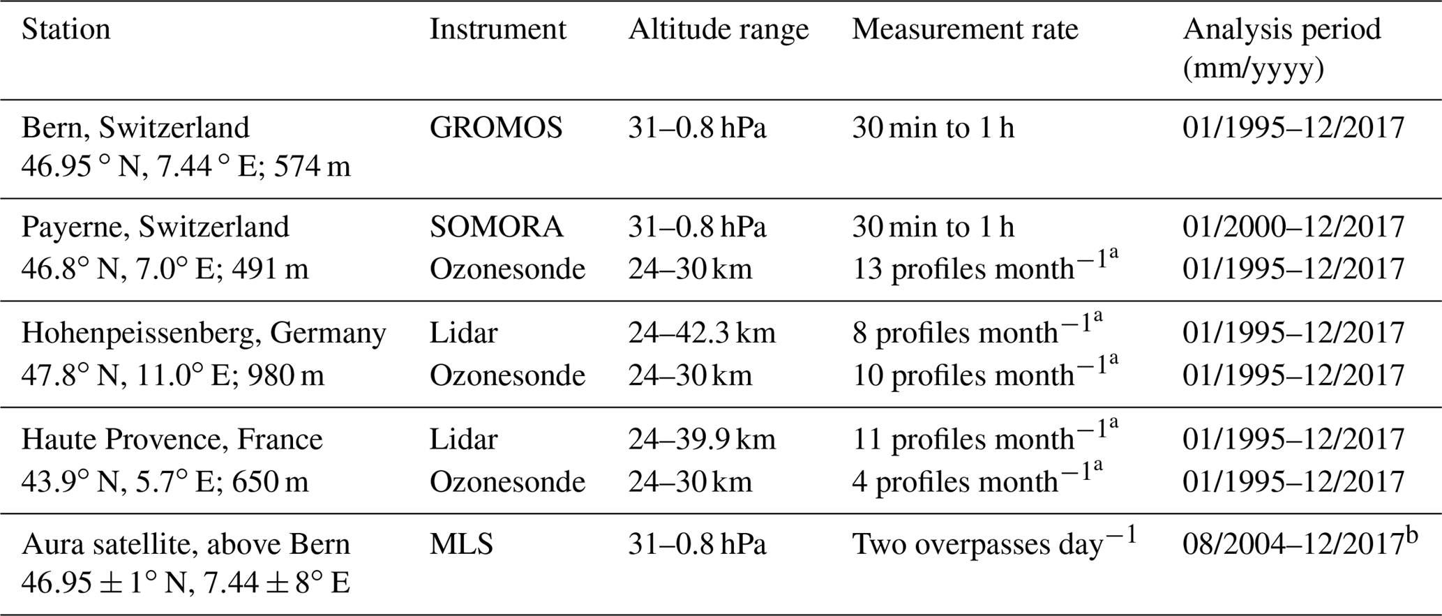
a Averaged number of profiles per month in the analysed period. b For the trend calculations, data from January 2005 to December 2017 are used.
2.1 Microwave radiometers
We use data from two microwave radiometers, both located in Switzerland. They measure the 142 GHz line where ozone molecules emit microwave radiation due to rotational transitions. The spectral line measured is pressure-broadened and thus contains information about the vertical distribution of ozone molecules. To obtain a vertical ozone profile, the received radiative intensity is compared to the spectrum simulated by the Atmospheric Radiative Transfer Simulator 2 (ARTS2; Eriksson et al., 2011). By using an optimal estimation method according to Rodgers (2000), the best estimate of the vertical profile of ozone volume mixing ratio is then retrieved from the measured spectrum. This is done using the software tool Qpack2, which together with ARTS2 provides an entire retrieval environment (Eriksson et al., 2005).
The GROund-based Millimetre-wave Ozone Spectrometer (GROMOS) located in Bern is the main focus of this study (Kämpfer, 1995; Peter, 1997). GROMOS has been measuring ozone spectra continuously since November 1994. Before October 2009, the measurements were performed by means of a filter bench (FB) with an integration time of 1 h. Since October 2009, a fast Fourier transform spectrometer (FFTS) with an integration time of 30 min has been used. An overlap measurement period of almost 2 years (October 2009 to July 2011) was used to homogenize the FB data, by subtracting the mean bias profile averaged over the whole overlap period (FBmean−FFTSmean) from all FB profiles (Moreira et al., 2015). These homogenized ozone data are available on the NDACC web page (ftp://ftp.cpc.ncep.noaa.gov/ndacc/station/bern/hdf/mwave/, last access: 28 March 2019). The FFTS retrieval used in the present study (version 2021) uses variable errors in the a priori covariance matrix of around 30 % in the stratosphere and 70 % in the mesosphere and a constant measurement error of 0.8 K (Moreira, 2017). The retrieved profiles have a vertical resolution of ∼ 15 to 25 km in the stratosphere. We concentrate in this study on the middle and upper stratosphere between 31 hPa (≈ 24 km) and 0.8 hPa (≈ 49 km), where the retrieved ozone is quasi-independent of the a priori information. This is assured by limiting the altitude range to the altitudes where the area of the averaging kernels (measurement response) is larger than 0.8, which means that more than 80 % of the information comes from the observation rather than from the a priori data (Rodgers, 2000). More information about the homogenization as well as the parameters used in the retrieval can be found in Moreira et al. (2015). Besides the described data harmonization to account for the instrument upgrade, we performed some additional data corrections. Because the stratospheric signal is weak in an opaque and humid troposphere, we discarded measurements when the atmospheric transmittance was smaller than 0.3. Excluding measurements in such a way should not result in a sampling bias because tropospheric humidity is uncorrelated to stratospheric ozone. Also, the data have been corrected for outliers at each pressure level by removing values that exceed 4 times the standard deviation within a 3-day moving median window. Profiles were excluded completely when more than 50 % of their values were missing (e.g. due to outlier detection). Furthermore, we omitted profiles in which the instrumental system temperature showed outliers exceeding 4 times the standard deviation within a 30-day moving median window.
The second microwave radiometer used in this study is the Stratospheric Ozone MOnitoring RAdiometer (SOMORA). It was built in 2000 as an update of the GROMOS radiometer and has been located in Payerne since 2002. Some instrumental changes were performed at the beginning of 2005 (front-end change) and in October 2010, when the acousto-optical spectrometer of SOMORA was upgraded to an FFTS (Maillard Barras et al., 2015). The data have been harmonized to account for the spectrometer change. The instrument covers an altitude range from 25 to 60 km with a temporal resolution of 30 min to 1 h. In this study, we consider SOMORA data at an altitude range between 18 hPa (≈ 27 km) and 0.8 hPa (≈ 49 km). For more information about SOMORA, refer to Calisesi (2003) concerning the instrumental setup and Maillard Barras et al. (2009, 2015) concerning the operational version of the ozone retrievals used in the present study.
2.2 Lidars
We use data from two differential absorption lidar (DIAL; Schotland, 1974) instruments in Germany and France. The instruments emit laser pulses at two different wavelengths, one of which is absorbed by ozone molecules and the other which is not. Comparing the backscattered signal at these two wavelengths provides information on the vertical ozone distribution in the atmosphere. The lidars can only retrieve ozone profiles during clear-sky nights due to scattering on cloud particles and the interference with sunlight.
The lidar at the Meteorological Observatory Hohenpeissenberg (MOH) has been operating since 1987, emitting laser pulses at 308 and 353 nm (Werner et al., 1983; Steinbrecht et al., 2009b). On average, it retrieves eight night profiles a month. In this study we limit the data to the altitude range in which the measurement error averaged over the whole study period is below 10 % (below 42 km or 2 hPa). The lower altitude limit was set to the chosen limit of GROMOS at 31 hPa (≈ 24 km).
The Observatory of Haute Provence (OHP) operates a lidar that has been measuring in its current setup since the end of 1993 (Godin-Beekmann et al., 2003). The lidar emits laser pulses at 308 nm and 355 nm, as first described by Godin et al. (1989). The instrument measures on average 11 profiles per month. We use OHP lidar profiles below 40 km (≈ 2.7 hPa) for which the averaged measurement error remains below 10 %. As a lower altitude limit, we use 31 hPa (≈ 24 km) to be consistent with the GROMOS limits. More detailed information about the lidars and ozonesondes used can be found, for example, in Godin et al. (1999) and Nair et al. (2011, 2012).
2.3 Ozonesondes
The three mentioned observatories at Payerne, MOH, and OHP also provide weekly ozonesonde measurements. The ozonesonde measurements in Payerne are usually performed three times a week at 11:00 UTC (Jeannet et al., 2007), resulting in 13 profiles per month on average. The meteorological balloon carried a Brewer Mast sonde (BM; Brewer and Milford, 1960) until September 2002, which was then replaced by an electrochemical concentration cell (ECC; Komhyr, 1969). The profiles are normalized using concurrent total column ozone from the Dobson spectrometer at Arosa, Switzerland (46.77∘ N, 9.7∘ E; 1850 m a.s.l.; Favaro et al., 2002). If the Dobson data are not available, forecast ozone column estimates based on GOME-2 (Global Ozone Monitoring Experiment–2) data are used (http://www.temis.nl/uvradiation/nrt/uvindex.php, last access: 28 March 2019).
Ozone soundings at MOH are performed two to three times per week with a BM sonde (on average 10 profiles per month). Three different radiosonde types have been used since 1995, all carrying a BM ozonesonde, without major changes in its performance since 1974 (Steinbrecht et al., 2016). The profiles are normalized by on-site Dobson or Brewer spectrophotometers and, if not available, by satellite data (Steinbrecht et al., 2016).
At OHP, ECC ozonesondes have been used since 1991 with several instrumental changes (Gaudel et al., 2015). The data were normalized with total column ozone measured by a Dobson spectrophotometer until 2007 and an ultraviolet–visible SAOZ (Système d'Analyse par Observation Zénithale) spectrometer afterwards (Guirlet et al., 2000; Nair et al., 2011). In our analysed period, four profiles are available on average per month.
Ozonesonde data are limited to altitudes up to ∼ 30 km, above which the balloon usually bursts. Therefore, we used ozonesonde profiles only below 30 km, which is a threshold value for Brewer Mast ozonesondes with precision and accuracy below ± 5 % (Smit and Kley, 1996). For normalization, the correction factor (CF), which is the ratio of total column ozone from the reference instrument to the total ozone from the sonde, has been applied to all ozonesonde profiles. At all measurement stations, we discarded profiles when their CF was larger than 1.2 or smaller than 0.8 (Harris et al., 1998; Smit and ASOPOS Panel, 2013). We further excluded profiles with extreme jumps or constant ozone values, as well as profiles with constant or decreasing altitude values.
2.4 Aura/MLS
The microwave limb sounder (MLS) on the Aura satellite, launched in mid-2004, measures microwave emission from the Earth in five broad spectral bands (Parkinson et al., 2006). It provides profiles of different trace gases in the atmosphere, with a vertical resolution of ∼ 3 km. Stratospheric ozone is retrieved by using the spectral band centred at 240 GHz. We used ozone data from Aura/MLS version 4.2 above Bern with a spatial coincidence of ±1 ∘ latitude and ±8 ∘ longitude, where the satellite passes twice a day (around 02:00 and 13:00 UTC). More information about the MLS instrument and the data product can be found, e.g. in Waters et al. (2006). We chose the Aura/MLS data for our study because there are no drifts between 20 and 40 km (Hubert et al., 2016).
To identify potential anomalies in the GROMOS data, we compared the data with the other described data sets in the time period from January 1995 to December 2017, except for some instruments that cover a shorter time period (Table 1).
3.1 Comparison methodology
To compare GROMOS with the other instruments, the different data sets have been processed to compare consistent quantities and have been smoothed to the GROMOS grid. Taking relative differences between the data sets made it possible to identify anomalous periods in the GROMOS time series.
3.1.1 Data processing
In this study we concentrate on the altitude range between 31 and 0.8 hPa, in which the a priori contribution to GROMOS profiles is low (see Sect. 2.1). We therefore limit all instrument data to this altitude range and divide it into three parts. For convenience, they will be referred to as the lower stratosphere between 31 and 13 hPa (≈ 24 to 29 km), the middle stratosphere between 13 and 3 hPa (≈ 29 to 39 km), and the upper stratosphere between 3 and 0.8 hPa (≈ 39 to 49 km). The limits for the upper stratosphere agree with the common definition (e.g. Ramaswamy et al., 2001), whereas the lower and middle stratosphere defined here are usually referred to as the middle stratosphere in other studies.
Most of the instruments provide volume mixing ratios (VMRs) of ozone in parts per million (ppm). In cases that the data were given in number density (molecules cm−3), the VMR was calculated with the air pressure and temperature provided by the same instrument for ozonesondes or co-located ozone- or radiosonde data for lidars. For lidar measurements, these sonde temperature and pressure profiles are completed above the balloon burst by operational model data from the National Center for Environmental Prediction (NCEP) at OHP and by lidar temperature measurements and extrapolated radiosonde pressure data at MOH.
The GROMOS, SOMORA, and Aura/MLS profiles have a constant pressure grid, which is not the case for the lidar and ozonesonde data. The lidar and ozonesonde data were therefore linearly interpolated to a regular spaced altitude grid of 100 m for the ozonesonde at OHP and Payerne and 300 m for the lidars and the ozonesonde at MOH. The mean profile of the interpolated pressure data then built the new pressure grid for the ozone data. These interpolated lidar and ozonesonde data are used for the trend estimations. For the direct comparison with GROMOS, the data were adapted to the GROMOS grid, which is described in the next section (Sect. 3.1.2). Our figures generally show both pressure and geometric altitude. The geometric altitude is approximated by the mean altitude grid from GROMOS, which is determined for each retrieved profile from operational model data of the European Centre for Medium-Range Weather Forecasts (ECMWF).
3.1.2 GROMOS comparison and anomalies
The vertical resolution of GROMOS and SOMORA is usually coarser than for the other instruments. When comparing profiles directly with GROMOS profiles, the different vertical resolution of the instruments has to be considered. Smoothing the profiles of the different instruments by GROMOS' averaging kernels makes it possible to compare the profiles with GROMOS without biases due to resolution or a priori information (Tsou et al., 1995). The profiles with higher vertical resolution than GROMOS were convolved by the averaging kernel matrix according to Connor et al. (1991), with
where xconv is the resulting convolved profile, xa is the a priori profile used in the GROMOS retrieval, xa,h is the same a priori profile but interpolated to the grid of the highly resolved measurement, xh is the profile of the highly resolved instrument, and AVK is the corresponding averaging kernel matrix from GROMOS. The rows of the AVK have been interpolated to the grid of the highly resolved instrument and scaled to conserve the vertical sensitivity (Keppens et al., 2015). The SOMORA profiles have a similar vertical resolution as profiles from GROMOS and were thus not convolved because this would require a more advanced comparison method as proposed by Rodgers and Connor (2003) or Calisesi et al. (2005). GROMOS and SOMORA have a higher temporal resolution than the other instruments. For SOMORA, only profiles coincident in time with GROMOS have been selected. For the other instruments, a mean of GROMOS data at the time of the corresponding measurement was used, with a time coincidence of ±30 min. Only for the lidars were GROMOS data averaged over the whole lidar measurement time (usually one night).
For comparison with GROMOS we computed relative differences between the monthly mean values of the different data sets and the monthly mean of the coincident GROMOS profiles. The relative difference (RD) for a specific month i has been calculated by subtracting the monthly ozone value of the data set (Xi) from the corresponding GROMOS monthly mean (GRi), using the GROMOS monthly mean as a reference:
Based on the relative differences we identified periods in which GROMOS differs from the other instruments. To identify these anomalies we used a debiased relative difference (RDdebiased), given by
where is the mean relative difference of GROMOS to the data set X over the whole period. This made it possible to ignore a potential constant offset of the instruments and to concentrate on periods with temporally large differences to GROMOS. When this debiased relative difference was larger than 10 % for at least three instruments, the respective month was identified as an anomaly in the GROMOS data. Above 2 hPa, for which only SOMORA and Aura/MLS data are available, both data sets need to have a debiased relative difference to GROMOS larger than 10 % to be identified as an anomaly.
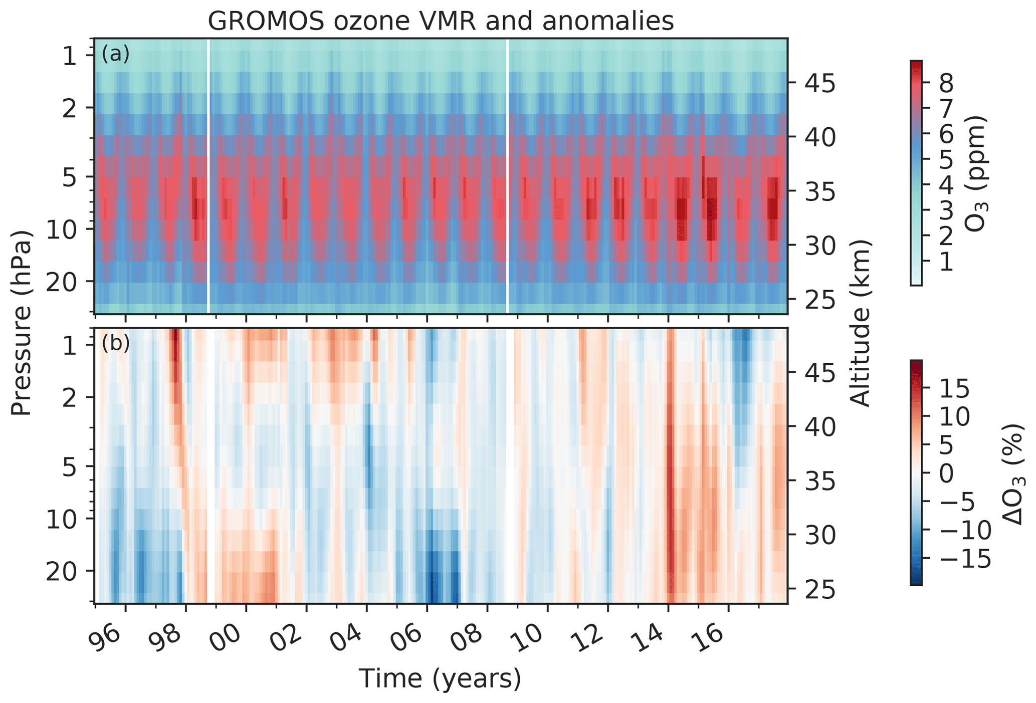
Figure 1(a) Monthly means of ozone volume mixing ratio (VMR) measured by GROMOS (Ground-based Millimetre-wave Ozone Spectrometer) at Bern from January 1995 to December 2017. The white lines indicate months for which no measurements were available due to instrumental issues. (b) Deviation from GROMOS monthly mean climatology (1997 to 2017), smoothed by a moving median window of 3 months.
3.2 GROMOS time series
The monthly means of the GROMOS time series (Fig. 1a) clearly depict the maximum of ozone VMR between 10 hPa and 5 hPa and the seasonal ozone variation, with increased spring–summer ozone in the middle stratosphere and increased autumn–winter values in the upper stratosphere (Moreira et al., 2016). Figure 1b shows GROMOS' relative deviations from the monthly climatology (monthly means over the whole period 1995 to 2017). This ozone deviation is calculated by the ratio of the deseasonalized monthly means (difference between each individual monthly mean and the corresponding climatology of this month) and the monthly climatology. We observe some periods in which GROMOS data deviate from their usual values, mostly distinguishable between the lower–middle stratosphere and the upper stratosphere. In the lower–middle stratosphere we observe negative anomalies (less ozone than usual) in 1995 to 1997 and 2005 to 2006 and positive anomalies (more ozone than usual) in 1998 to 2000, in 2014 to 2015, and in 2017. In the upper stratosphere the data show negative anomalies in 2016 and positive anomalies in 2000 and 2002 to 2003. Strong but short-term positive anomalies are visible in 1997 in the upper stratosphere and at the beginning of 2014. The positive anomaly in the upper stratosphere in 1997 is due to some missing data in November 1997 because of an instrumental upgrade, leading to a larger monthly mean value than usual. Besides this we did not detect any systematic instrumental issues in the GROMOS data that could explain the anomalies. Therefore, we compare the GROMOS data with the presented ground-based data sets, as well as with Aura/MLS data, to check whether the observed anomalies are due to natural variability or due to unexplained instrumental issues.
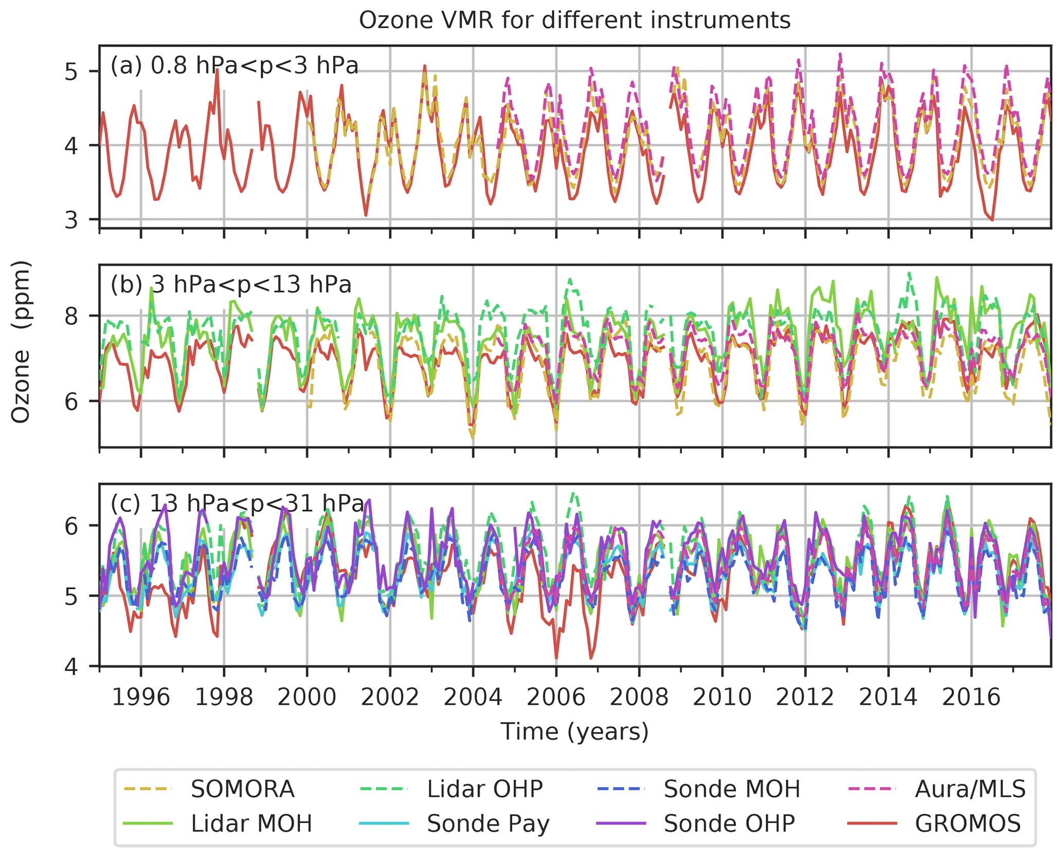
Figure 2Monthly means of ozone VMR from the microwave radiometers GROMOS (Bern) and SOMORA (Payerne), the lidars at the observatories of Hohenpeissenberg (MOH) and Haute Provence (OHP), and the ozonesonde measurements at MOH, OHP, and Payerne, as well as Aura/MLS data above Bern. The data have been averaged over three altitude ranges.
3.3 Comparison of different data sets
We compared GROMOS with ground-based and Aura/MLS data and averaged them over three altitude ranges (Fig. 2). The different data sets have been smoothed with the averaging kernels of GROMOS to make a direct comparison possible, as described in Sect. 3.1.2. Due to the similar vertical resolution of GROMOS and SOMORA, the SOMORA profiles have not been smoothed by GROMOS' averaging kernels, despite differences between their a priori data and averaging kernels. This might lead to larger differences between GROMOS and SOMORA than between GROMOS and the other instruments. To avoid an instrument not covering the full range of one of the three altitude ranges, all ozonesonde data have been cut at 30 km (≈ 11.5 hPa), all lidar data at 3 hPa (≈ 39 km), and all SOMORA data below 13 hPa (≈ 29 km) for this analysis. The different instrument time series shown in Fig. 2 only contain data that are coincident with GROMOS measurements as described in Sect. 3.1.2, whereas the GROMOS data shown here represent the complete GROMOS time series with its high temporal sampling. This might lead to some sampling differences that are not considered in this figure.
The different data sets agree well, showing, however, periods in which some instruments deviate more from GROMOS than others. In the upper stratosphere (Fig. 2a), GROMOS and SOMORA agree well most of the time, but GROMOS reports slightly less ozone than SOMORA and also smaller values than Aura/MLS. A step change between SOMORA and GROMOS is visible in 2005, which might be related to the SOMORA front-end change in 2005. In the middle stratosphere (Fig. 2b), both lidars exceed the other instrument data in the last years, starting in 2004 at OHP and in 2010 at MOH. Similar deviations of the MOH and OHP lidars have also been observed by Steinbrecht et al. (2017), as can be seen in the latitudinal lidar averages of their study.

Figure 3Relative differences (RD) of monthly means between GROMOS and coincident pairs of SOMORA, lidars (MOH, OHP), ozonesondes (Payerne, MOH, OHP), and Aura/MLS, averaged over three altitude ranges. The relative difference (RD) is given by , where GR represents GROMOS monthly means and X represents monthly means of the other data sets. The black lines show the mean values of all RDs, and the grey shaded areas show its standard deviation.
Differences between the data sets in the lower stratosphere can be better seen in Fig. 3. The monthly relative differences of time coincident pairs of GROMOS (GR) and the convolved data set X are shown, with GROMOS data as reference values (Eq. 2). The mean relative difference of all instruments compared to GROMOS (black line in Fig. 3) generally lies within %. However, there are some periods with larger deviations, in which GROMOS measures less ozone than the other instruments (negative relative difference) in 1995 to 1997 and in 2006 in the lower stratosphere and in 2016 in the middle and upper stratosphere. We further observe that the relative difference between GROMOS and the OHP ozonesonde shows some important peaks in the last decade, indicating that the sonde often measures more ozone than GROMOS. The ozonesonde data seem to have some outlier profiles. When comparing the monthly means of coincident pairs, these outliers are even more visible because only a small number of OHP ozonesonde profiles are available per month (only four profiles on average).
For a broader picture, the same relative differences to GROMOS are shown in Fig. 4, but each panel represents an individual instrument, and all altitude levels are shown. The anomalies for which at least three data sets (or two above 2 hPa) deviate by more than 10 % from GROMOS (as described in Sect. 3.1.2) are shown in the lowest panel in black. In addition to the negative anomalies observed already in the other figures (e.g. in 2006 in the lower stratosphere and in 2016 in the upper stratosphere), we also observe positive anomalies in the lower–middle stratosphere in 2000 and 2014. The negative anomalies in 1995 to 1997 in the lower stratosphere that we observed in Fig. 3 were only partly detected as anomalies with our anomaly criteria.
To summarize our comparison results, we observed some periods with anomalies compared to GROMOS' climatology (Fig. 1). Some of these anomalies were also observed when comparing GROMOS to the different data sets (Figs. 2, 3, and 4). This implies that the source of the anomalies is local variations in Bern or instrumental issues of GROMOS rather than broad atmospheric variability. We can thus conclude that the observed negative GROMOS anomalies in the lower stratosphere in 2006 and in the upper stratosphere in 2016 are biases in the GROMOS time series. The same is the case for the positive anomalies in 2000 and 2014 in the lower and middle stratosphere and also for some summer months in 2015, 2016, and 2017. In contrast to these confirmed anomalies, the GROMOS anomalies in the lower stratosphere in 1995 to 1997 (negative) and 1998 and 1999 (positive) as observed in Fig. 1 are small when comparing to the other instruments and are thus only confirmed for a few months by our anomaly detection. The biased periods in the upper stratosphere in 2000 and 2002 to 2003 (positive anomalies) were not confirmed by comparing GROMOS to SOMORA and might thus be real ozone variations. However, we have to keep in mind that fewer instruments (only SOMORA and Aura/MLS) provide data for comparison above 2 hPa, which makes the anomaly detection less robust at these altitudes, especially prior to the start of Aura/MLS measurements in 2004. Our results are consistent with those reported by Moreira et al. (2017). They compared GROMOS with Aura/MLS data and also observed positive deviations of GROMOS in the middle stratosphere in 2014 and 2015 as well as a negative deviation in the upper stratosphere in 2016. Hubert et al. (2019) found similar anomalies in the GROMOS time series by comparing ground-based data sets to several satellite products (see also SPARC/IO3C/GAW, 2019). Some of our detected biased periods were also found by Steinbrecht et al. (2009a) who compared different ground-based instruments, for example, the GROMOS anomaly in 2006. They attribute the observed biases to sampling differences but also to irregularities in some data sets. In fact, our results confirm irregularities in the GROMOS time series, which are probably due to instrumental issues of GROMOS and not only due to sampling differences.
Ozone trends are estimated in the present study by using a multilinear parametric trend model (von Clarmann et al., 2010). By comparing the GROMOS data to the other data sets as described above (Sect. 3.3), we have confirmed some anomalous periods in the GROMOS time series. To improve the GROMOS trend estimates, we now use these detected anomalies and consider them in the regression fit. In the following, the trend model (Sect. 4.1) will first be applied to an artificial time series to test and illustrate the approach of considering anomalies in the regression (Sect. 4.2). It will then be applied on GROMOS data (Sect. 4.3) before comparing the resulting GROMOS trends to trends from the other instruments (Sect. 4.4).
4.1 Trend model
To estimate stratospheric ozone trends, we applied the multilinear parametric trend model from von Clarmann et al. (2010) to the monthly means of all individual data sets. The model fits the following regression function:
where y(t) represents the estimated ozone time series, t is the monthly time vector, and a to h are coefficients that are fitted in the trend model. QBO30 hPa and QBO50 hPa are the normalized Singapore winds at 30 and 50 hPa, used as indices of the quasi-biennial oscillation (QBO, available at http://www.geo.fu-berlin.de/met/ag/strat/produkte/qbo/singapore.dat, last access: 28 March 2019). F10.7 is the solar flux at a wavelength of 10.7 cm used to represent the solar activity (measured in Ottawa and Penticton, Canada; National Research Council of Canada, 2019). The El Niño Southern Oscillation (ENSO) is considered by the Multivariate ENSO Index (MEI), that combines six meteorological variables measured over the tropical Pacific (Wolter and Timlin, 1998). The F10.7 data and the MEI data are available via https://www.esrl.noaa.gov/psd/data/climateindices/list/ (last access: 28 March 2019). In addition to the described natural oscillations, we used four periodic oscillations with different wavelengths ln to account for annual (l1=12 months) and semi-annual (l2=6 months) oscillation as well as two further overtones of the annual cycle (l3=4 months and l4=3 months).
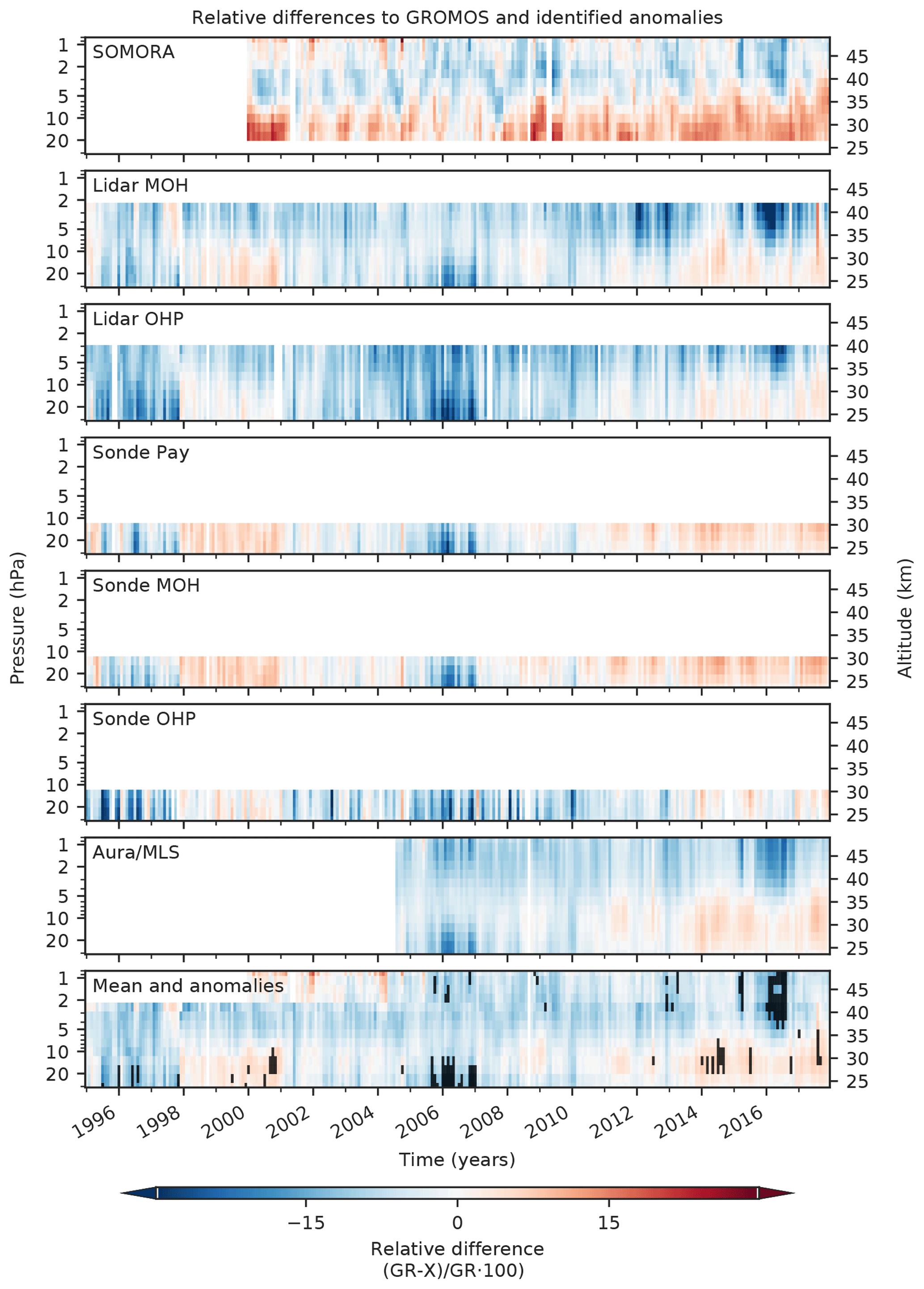
Figure 4Relative differences (RDs) of monthly means between GROMOS and SOMORA, lidars (MOH and OHP), ozonesondes (Payerne, MOH, OHP), and Aura/MLS. The lowest panel shows the mean of all RDs. The black areas in the lowest panel show periods in which at least three data sets (or two data sets above 2 hPa) have a debiased relative difference (RDdebiased) larger than 10 %.
The strength of the model from von Clarmann et al. (2010) used in our study is that it can consider inhomogeneities in data sets, by considering a full error covariance matrix (Sy) when reducing the cost function (χ2). Inhomogeneous data can originate from changes in the measurement system (e.g. changes in calibration standards or merging of data sets with different instrumental modes), from irregularities in spatial or temporal sampling, or from unknown instrumental issues. Such inhomogeneities lead to groups of temporally correlated data errors, that can, if not considered, change significance and slope of the estimated trend (von Clarmann et al., 2010). The study of von Clarmann et al. (2010) presents an approach to consider known or suspected inhomogeneities in the trend analysis. They divide the data into multiple subsets which are assumed to be biased with respect to each other and which are characterized by diagonal blocks in the data covariance matrix. We use their method and code in our trend analyses to account for inhomogeneities. The inhomogeneities are in our case anomalies in some months that we identified as described in Sect. 3.1.2.
The total uncertainty of the data set is represented by a full error covariance matrix Sy that describes covariances between the measurements in time for each pressure level. The covariance matrix is for each instrument given by
where Sinstr gives the monthly uncertainty estimates for the instrument, Sautocorr accounts for residuals autocorrelated in time which are caused by atmospheric variation not captured by the trend model, and Sbias describes the bias uncertainties when a bias is considered. The diagonal elements of Sinstr are set to the monthly means of the measurement uncertainties for each instrument. For lidar data this is on average 4 % for the OHP lidar and 6 % at MOH between ∼ 20 and 40 km, with smallest uncertainties in the middle stratosphere. For the ozonesonde, the uncertainty is assumed to be 5 % for all ECC sondes and 10 % for BM sondes (Harris et al., 1998; Smit and ASOPOS Panel, 2013). For SOMORA we use uncertainties composed of smoothing and observational error, ranging from 1 % to 2 % in the middle stratosphere and 2 % to 7 % in the upper stratosphere. The Aura/MLS uncertainties used range between 2 % and 5 % throughout the stratosphere. For GROMOS we use uncertainty estimates as described by Moreira et al. (2015), composed of the standard error (, with standard deviation σ and degrees of freedom DOF) of the monthly means, an instrumental uncertainty (measurement noise), and an estimated systematic instrument uncertainty obtained from cross-comparison. The resulting uncertainty values are approximately 5 % in the middle stratosphere, 6 % to 8 % in the lower stratosphere, and 6 % to 7 % in the upper stratosphere. The off-diagonal elements of Sinstr are set to zero, assuming no error correlation between the measurements in time. The additional covariance matrix Sautocorr, which is added to Sinstr, is first also set to zero. In a second iteration, autocorrelation coefficients are inferred from residuals of the initial trend fit. The mean variance of Sautocorr is scaled such that the χ2 divided by the degrees of freedom of the trend fit with the new Sy becomes unity. The degrees of freedom are the number of data points minus the number of fitted variables. The latter are the number of the coefficients of the trend model plus the number of relevant correlation terms inferred by the procedure described above. This additional covariance matrix Sautocorr represents contributions to the fit residuals which are not caused by data errors but by phenomena that are not represented by the trend model. Sautocorr is only considered if the initial normalized χ2 is larger than unity, which is not the case if the assumed data errors are larger than the fit residuals (Stiller et al., 2012). The more sophisticated uncertainty estimates that we use for GROMOS are larger than the residuals in the first regression fit (χ2<1), which means that the time correlated residuals (Sautocorr) are not considered for the GROMOS trend. For all the other instruments, however, correlated residuals are considered because we use simple instrumental uncertainties that are usually smaller than the fitted residuals.
To account for the anomalies in the time series when estimating the trends we adapted Sy in two steps. First, we increased the uncertainties for months and altitudes for which anomalies were identified (using the method described in Sect. 3.1.2). For this purpose, we set the diagonal elements of Sinstr for the respective month i to a value obtained from the mean difference to all instruments (RDdebiased,i) and the mean GROMOS ozone value. Assuming, for example, that GROMOS deviates from all instruments on average by 10 % in August 2014 at 10 hPa, the overall mean August value at this altitude would be 7 ppm. In this case we would assume an uncertainty of 0.7 ppm for this biased month at this altitude level. In a second step, we account for biases in the data subsets in which anomalies were detected. For this, a fully correlated block composed of the squared estimated bias uncertainties is added to the part of Sbias that is concerned by anomalies. For example, to account for a bias in the summer months of 2014, a fixed bias uncertainty is added to all variances and covariances of these months in Sbias. Considering the bias in this way is mathematically equivalent to treating the bias as an additional fit variable that is fitted to the regression model with an optimal estimation method, as shown by von Clarmann et al. (2001). The value chosen for the bias uncertainty determines how much the bias is estimated from the data itself. For small values, the bias will be close to the a priori value, which would be a bias of zero; for large values it will be estimated completely from the given data. The bias can thus be estimated from the data itself, which makes the method more robust because it does not depend on an a priori choice of the bias (Stiller et al., 2012). In a sensitivity test we found that assuming an uncertainty value of 5 ppm for the correlated block permits a reliable fit, whereby the bias is fitted independently of the a priori zero bias.
The described procedure for anomaly consideration is only applied to the GROMOS time series, whereas the other trend estimates were not corrected for anomalies. Our ozone trend estimates always start in January 1997, which is the most likely turning point for ozone recovery due to the decrease of ODSs (Jones et al., 2011), and all end in December 2017. Exceptions are the trends from SOMORA and Aura/MLS. The SOMORA trend starts in January 2000 when the instrument started to measure ozone. Aura/MLS covers the shortest trend period, starting only in January 2005. The trends are always given in % decade−1, which is determined at each altitude level from the regression model output in ppm decade−1 by dividing it for each data set by its ozone mean value of the whole period. We declare a trend to be significantly different from zero at a 95 % confidence interval, as soon as its absolute value exceeds twice its uncertainty. This statistically inferred confidence interval is based on the assumed instrumental uncertainties. Unknown drifts of the data sets, however, are not considered in this claim.
4.2 Artificial time series analysis
The trend programme from von Clarmann et al. (2010) can handle uncertainties in a flexible way, which makes it possible to account for anomalies in a time series, as described above (Sect. 4.1). To investigate how anomalies can be best considered in the trend programme, we first test the programme with a simple artificial time series and then try to use the specific features of the trend programme to immunize it against anomalies. The artificial time series used for this purpose consists of monthly ozone values from January 1997 to December 2017 and is given by
with the monthly time vector t, a constant ozone value a=7 ppm, and a trend of 0.1 ppm decade−1, i.e. ppm per month. We consider a simple seasonal oscillation with an amplitude A=1 ppm such that (e.g. ppm) and a wavelength ln=12 months. The uncertainty was assumed to be 0.1 ppm for each monthly ozone value, which was considered in the diagonal elements of Sy. No noise was superimposed to the data. This artificial time series (shown in Fig. 5a) is later on referred to as case A. The estimated trend for this simple time series corresponds quasi-perfectly to the assumed time series' trend (0.1 ppm decade−1), which proves that the trend programme works well. The residuals are of order 10−6 and increase towards the start and end of the time series (Fig. 5b).
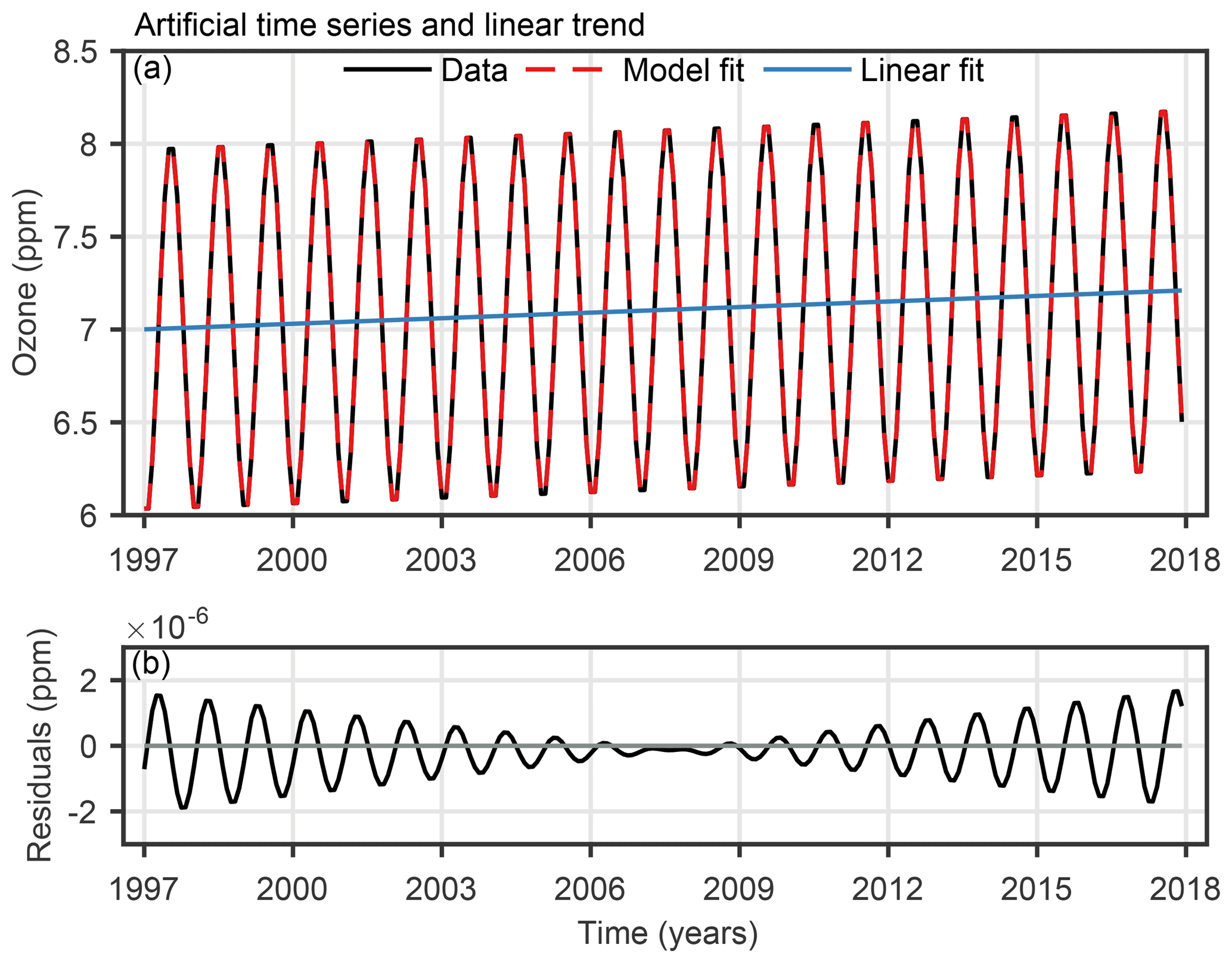
Figure 5(a) Artificial ozone time series (composed of a simple seasonal cycle and a linear trend) and its model fit and linear trend estimation. (b) Trend model residuals (data − model fit).
To investigate how the trend programme reacts to anomalies in the time series, we performed the following sensitivity study. We increased the monthly ozone values in the summer months (June, July, August) of 2014, 2015, and 2017 by 5 % (≈ 0.4 ppm). Since we are interested in the net effect of the anomalies, again no noise was superimposed on the test data. The same error covariance matrix Sy as in case A has been used. For this modified time series (case B), we observe a trend of ∼ 0.13 ppm decade−1 instead of the expected ∼ 0.1 ppm decade−1 (Fig. 6 and Table 2). Assuming that a real time series contains such suspicious anomalies due to, for example, instrumental issues, they would distort the true trend.
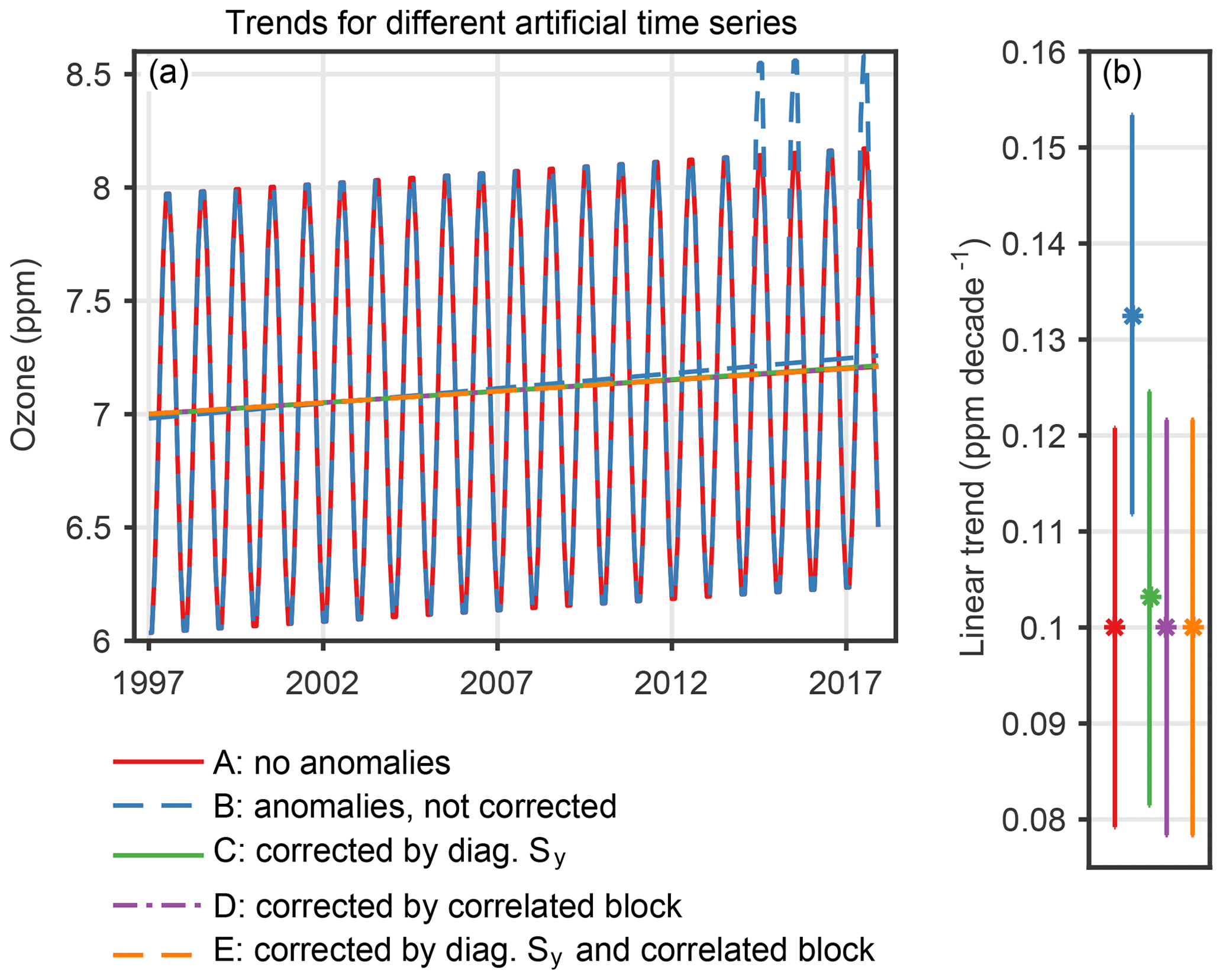
Figure 6(a) Ozone time series and linear trends for the same artificial ozone time series as in Fig. 5 (case A). Anomalies were added to the time series in the summer months 2014, 2015, and 2017 in case B. Different corrections have been applied to account for those anomalies in the trend fit, represented by cases C to E. (b) Linear trend estimates for the time series without anomalies (case A) and the time series with added anomalies, for which the anomalies were considered in different ways (cases C, D, E) or not considered at all (case B). The error bars show 2 standard deviation (σ) uncertainties.
Table 2Summary of the artificial ozone time series and the different model parameters used to correct the trend estimation for artificially added anomalies.
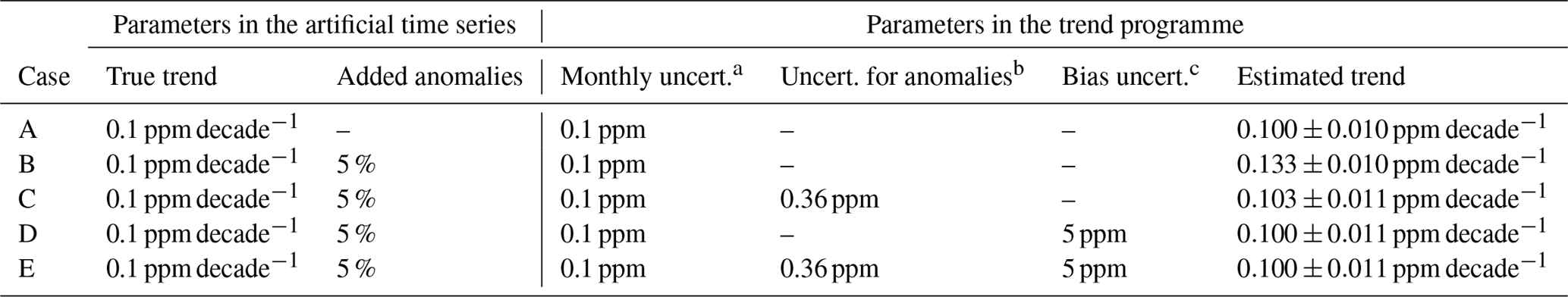
a Uncertainty considered in the diagonal elements of the covariance matrix Sy. b Uncertainty considered in the diagonal elements of Sy for months with anomalies. c Bias uncertainty considered in the off-diagonal elements of Sy for months with anomalies, set as a correlated block.
A simple way to handle such anomalies would be to omit anomalous data in the time series. This, however, would increase trend uncertainties and lead to a loss of important information. Therefore, we use the presented approach to handle anomalous observations in the time series when estimating the trend. To account for these anomalies in the trend estimation, we make use of the fact that the user of the trend programme has several options to manipulate the error covariance matrix Sy. In a first attempt we decreased the weight of the anomalies in the time series by increasing their uncertainties (diagonal elements of Sy) and set the uncertainties of the affected summer months to 0.36 ppm (case C in Fig. 6 and Table 2). This uncertainty value corresponds to 5 % of the overall mean ozone value. The uncertainty of the months without anomalies remained 0.1 ppm. No additional error correlations between the anomaly-affected data points were considered. The impact of the anomaly is already reduced from about 33 % to about 3 %. The estimated error of the trend has slightly increased because, with this modified covariance matrix which represents larger data errors, the data set contains less information.
In a next step, we added a correlated block to the covariance matrix for the months containing anomalies and applied the Sy once without (case D) and once with (case E) the increased diagonal elements of Sy. Adding the correlated block to Sy corresponds to an unknown bias of the data subset that is affected by anomalies and leads to a free fit of the bias magnitude. This bias is represented in Sy as a fully correlated block of (5 ppm)2. It has an expectation value of zero and an uncertainty of 5 ppm. With this approach (cases D and E), the trend obtained from the anomaly-affected data is almost identical to the trend obtained from the original data (case A). This implies that the trend estimation has successfully been immunized against the anomaly.
In summary, we found that the trend estimates based on anomaly-affected data are largely improved by consideration of the anomalies in the covariance matrix, while without this, a largely erroneous trend is found. For this purpose it is not necessary to know the magnitude of the systematic anomaly. It is only necessary to know which of the data points are affected. We further found that the trend estimate is closer to its true value when higher uncertainties are chosen (diagonal elements of Sy or correlated block in Sy; not shown). This can be explained by the fact that the additional uncertainties represented by Sy allow the bias to vary as in an optimal estimation scheme in which the bias is a fit variable itself (von Clarmann et al., 2001). When estimating the bias, the larger the bias uncertainty is, the less confidence is accounted to the a priori knowledge about the bias (that would be a bias of zero), and the bias is then determined directly from the data as if it were an additionally fitted variable. Based on our test with the artificial time series, we conclude that our method succeeds in handling suspicious anomalies in a time series, leading to an estimated trend close to the trend that would be expected without anomalies.
4.3 GROMOS trends
The GROMOS time series has been used for trend estimations in Moreira et al. (2015), who found a significant positive trend in the upper stratosphere. In recent years, GROMOS showed some anomalies leading to larger trends than expected in the middle atmosphere, as, for example, shown by Steinbrecht et al. (2017) or SPARC/IO3C/GAW (2019). These larger trends motivated us to improve GROMOS trend estimates by accounting for the observed anomalies. In the following, we present the trend profiles of the GROMOS time series by considering the detected anomalies in the trend programme with the different correction methods that were introduced in Sect. 4.1. In a first step, we estimated the trend without considering anomalies in the data (case I in Fig. 7). The uncertainties of the data that are used as diagonal elements in Sy range between 5 % and 8 % and are composed as proposed by Moreira et al. (2015) (see Sect. 4.1). In a second step (case II), we increased the uncertainties (diagonal elements of Sy) for the months and altitudes that were detected as anomalies. The uncertainties for these anomalous data have been set to a value obtained from the difference to the other data sets (RDdebiased), as described in Sect. 4.1. Finally, we considered a fully correlated block for the periods in which anomalies were detected to fit a bias (case III). The bias uncertainty was set to 5 ppm at all altitudes, which ensures that the bias is fully estimated from the data. The diagonal elements of Sy stayed the same as in case II.
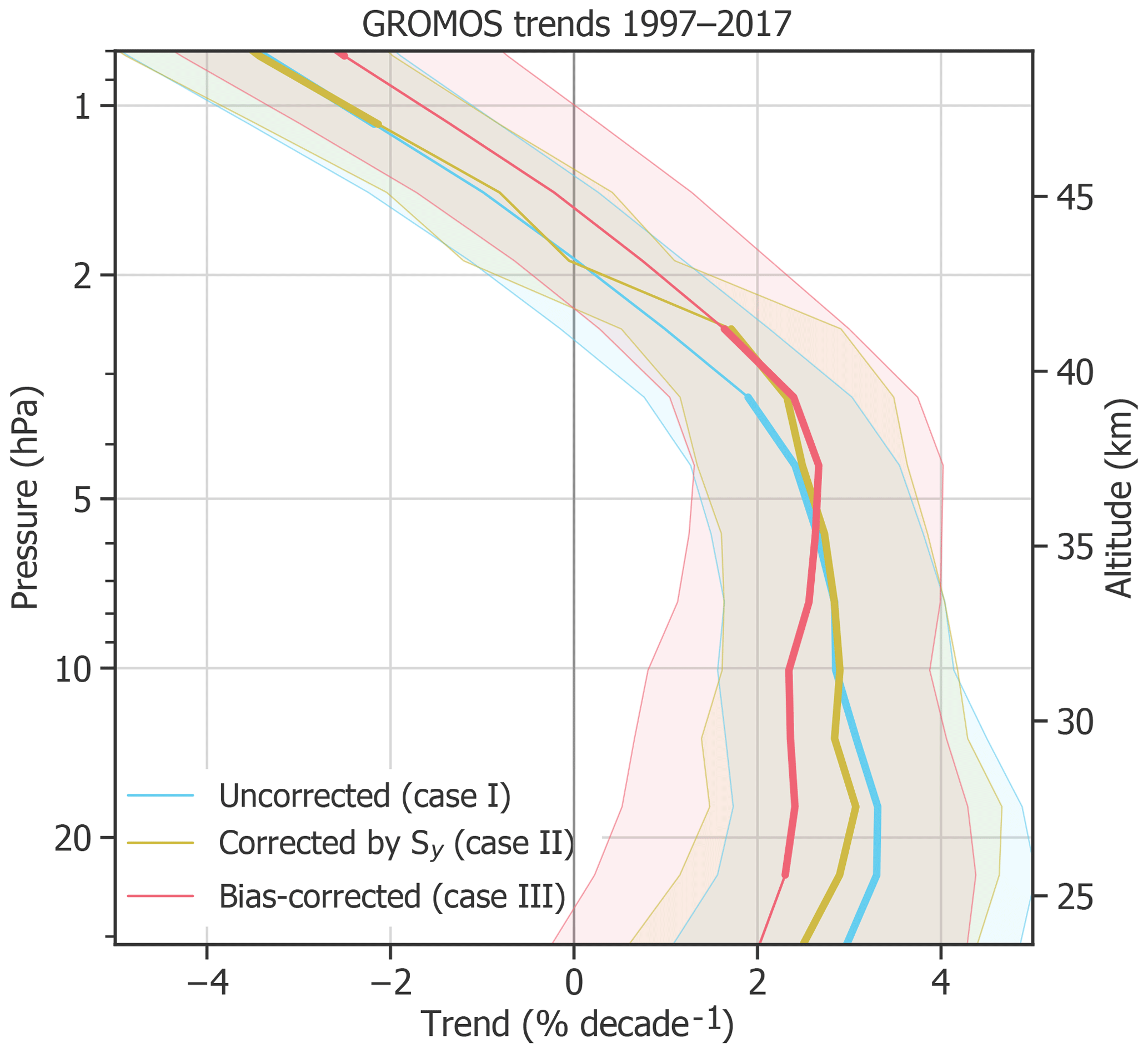
Figure 7GROMOS ozone trends from January 1997 to December 2017, without considering anomalies (case I), considering anomalies in the diagonal elements of Sy (case II), and considering a correlated bias block for anomalies (case III). The shaded areas show 2σ uncertainties, whereas the bold lines represent altitudes at which the trend profile is significantly different from zero at a 95 % confidence interval ().
The trend profiles in Fig. 7 report an uncorrected GROMOS ozone trend (case I) of about 3 % decade−1 in the middle stratosphere from 31 to 5 hPa, which decreases above to around −4 % decade−1 at 0.8 hPa. Correcting the trend by increasing the uncertainty for months with anomalies (case II) decreases the trend slightly in the lower stratosphere, but the differences are small. Using a correlated block in the covariance matrix to estimate the bias of each anomaly in an optimized way (case III) decreases the trend by around 1 % decade−1 in the lower stratosphere. The trend profile of this optimized trend estimation has a trend of 2.2 % decade−1 in the lower and middle stratosphere and peaks at approximately 4 hPa with a trend of 2.7 % decade−1. The corrected trend profile is consistent with recent satellite-based ozone trends (e.g. Steinbrecht et al., 2017) in the middle stratosphere. In the upper stratosphere it decreases again to −2.4 % decade−1 at 0.8 hPa.
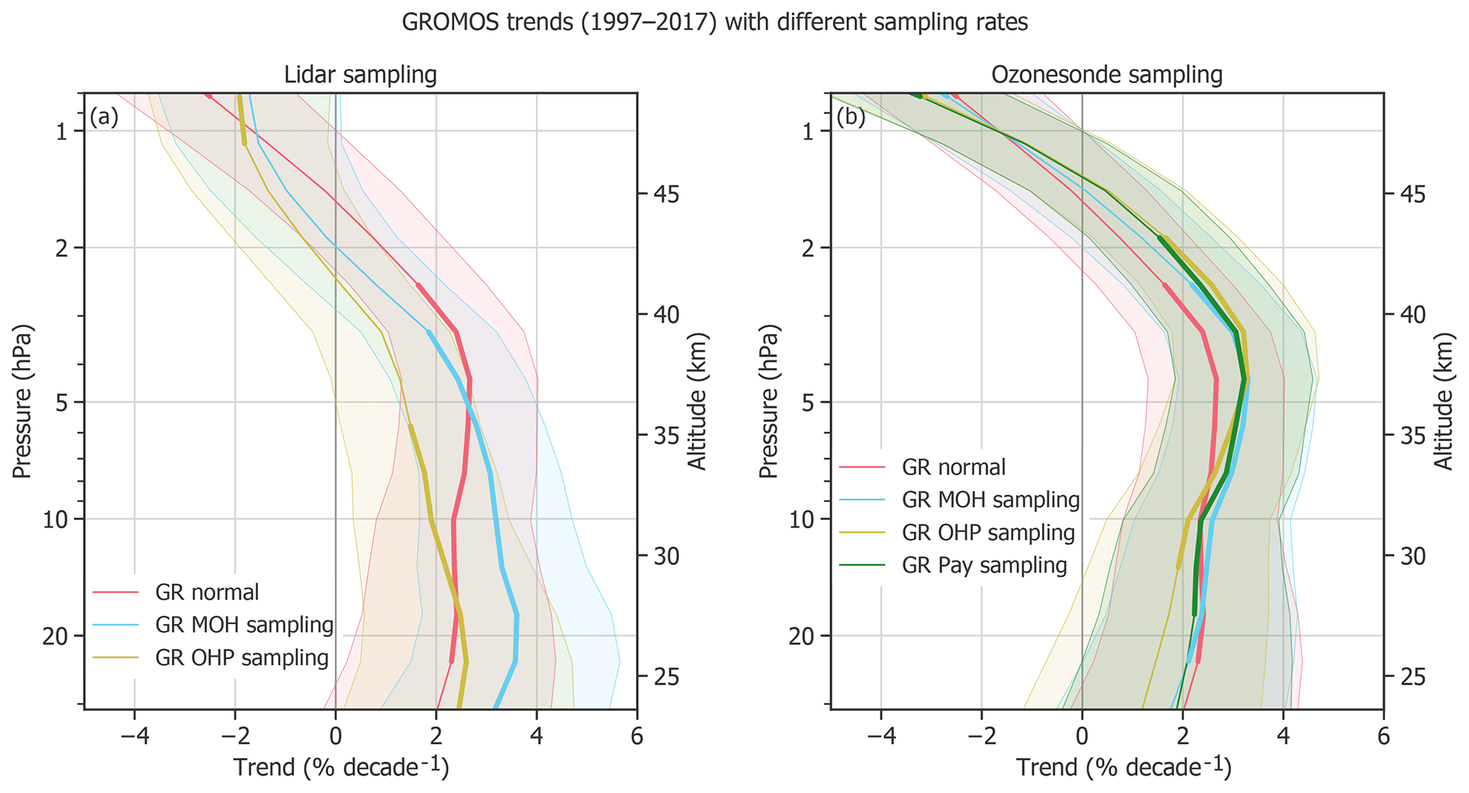
Figure 8GROMOS (GR) trends from January 1997 to December 2017 using its high temporal resolution (normal data set with correction for anomalies) as well as the temporal sampling rate of the different lidars (a) and ozonesondes (b). The shaded areas show the 2σ uncertainties, and bold lines identify trends that are significantly different from zero.
All these different GROMOS trend estimates, considering anomalies in different ways, show a significant positive trend of ∼ 2.5 % decade−1 at around 4 hPa (≈ 37 km) and a trend decrease above. This agreement indicates that the trend at these altitudes is only marginally affected by the identified anomalies and is rather robust. We can thus conclude that the trend of around 2.5 % decade−1 is a sign for an ozone recovery in the altitude range of 35 to 40 km. This result is consistent with trends derived from merged satellite data sets as, for example, found in Ball et al. (2017), Frith et al. (2017), Sofieva et al. (2017), or Steinbrecht et al. (2017), even though the GROMOS trend peak is observed at slightly lower altitudes. A possible reason for this difference in the trend peak altitude might be related to the averaging kernels of the current GROMOS retrieval version. We observe that after the instrument upgrade in 2009, the averaging kernels peak at higher altitudes than expected, indicating that the information is retrieved from slightly higher altitudes (∼ 2 to 4 km). It is therefore possible that the trend peak altitude does not exactly correspond to the true peak altitude. The instrumental upgrade in 2009 led to a change in the averaging kernels. This change, however, should not influence the trend estimates because the data have been harmonized (see Sect. 2.1) and thus corrected for such effects. The harmonization also corrects for possible effects due to changes in the temporal resolution (from 1 h to 30 min).
In the upper stratosphere (above 2 hPa), the GROMOS trend estimates are mostly insignificant but negative. This is probably influenced by the negative trend observed in the mesosphere. A negative ozone trend in the mesosphere is consistent with theory because increased methane emissions lead to an enhanced ozone loss cycle above 45 km (WMO, 2014). However, this is not further investigated in the present study because of the small mesospheric measurement response in the GROMOS filter bench data (before 2009).
In the middle and lower stratosphere (below 5 hPa), using different anomaly corrections results in largest trend differences, with trends ranging from 2 % decade−1 to 3 % decade−1. This result suggests that the GROMOS anomalies mostly affect these altitudes between 30 and 5 hPa. The corrected GROMOS trend (case III) is not significantly different from zero below 23 hPa, but cases I (uncorrected) and II (corrected by Sy) show significant trends. Compared to other studies, the GROMOS trends in the lower stratosphere are slightly larger than trends of most merged satellite data sets.
In summary, correcting the GROMOS trend with our anomaly approach leads to a trend profile of ∼ 2 % decade−1 to 2.5 % decade−1 in the lower and middle stratosphere. This is consistent with satellite-based trends from recent studies in the middle stratosphere but is still larger than most satellite trends in the lower stratosphere. The GROMOS trends are almost not affected by anomalies at 4 hPa (≈ 37 km), suggesting a robust ozone recovery of 2.5 % decade−1 at this altitude. At lower altitudes, trends are more affected by the detected anomalies, and the corrected trend estimate shows a trend of 2 % decade−1. The larger uncertainties in the lower stratosphere, the dependency on anomalies, and the insignificance of the corrected trend show that this positive trend in the lower stratosphere is less robust than the trend at higher altitudes.
4.3.1 Influence of temporal sampling on trends
Stratospheric ozone at northern mid-latitudes has a strong seasonal cycle of ∼ 16 % (Moreira et al., 2016) and a moderate diurnal cycle of 3 % to 6 % (Schanz et al., 2014; Studer et al., 2014). The sampling rate of ozone data is thus important for trend estimates because measurement dependencies on season or time of the day might influence the resulting trends. An important characteristic of microwave radiometers is their measurement continuity, being able to measure during day and night as well as during almost all weather conditions (except for an opaque atmosphere) and thus during all seasons. Other ground-based instruments such as lidars are temporally more restricted because they typically acquire data during clear-sky nights only. Clear-sky situations are more frequent during high-pressure events which vary with season and location (Steinbrecht et al., 2006; Hatzaki et al., 2014). The lidar measurements thus do not only depend on the daily cycle, but also on location and season. The seasonal dependency for ozonesondes might be smaller, but they are only launched during daytime.
Figure 8 gives an example of how the measurement sampling rate can influence resulting trends. The GROMOS time series is used for these trend estimates, once using only measurements at the time of lidar measurements and once only at the time of ozonesonde launches. The differences to the trend that uses the complete GROMOS sampling are not significant but still important, especially between 35 and 40 km and in the lower stratosphere. Using the sampling of the MOH lidar leads to larger trends (∼ 3 % decade−1) than using the normal sampling (∼ 2 % decade−1) below 5 hPa. The OHP lidar sampling, however, leads to smaller trends than the normal sampling above 13 hPa. This suggests that selecting different night measurements within a month can lead to trend differences.
All three ozonesonde samplings result in a larger trend than normal or lidar sampling above 5 hPa. Even if ozonesondes are not measuring at those altitudes, the result shows that measuring with an ozonesonde sampling (e.g. only at noon) might influence the trend at these altitudes. Our findings suggest that the time of the measurement (day or night) or the number and the timing of measurements within a month can influence the resulting trend estimates. Results concerning the time dependences of trends based on SOMORA data can be found in Maillard Barras et al. (2019). We conclude that sampling differences have to be kept in mind when comparing trend estimates from instruments with different sampling rates or measurement times.
4.3.2 Influence of time period on trends
An important factor that influences trend estimates is the length and starting year of the trend period. Several studies have shown that the choice of start or end point affects the resulting trend substantially (Harris et al., 2015; Weber et al., 2018). Further, the number of years in the trend period is crucial for the trend estimate (Vyushin et al., 2007; Millán et al., 2016). We investigate how the GROMOS trends change when the regression starts in different years. For this, we average the GROMOS trends over three altitude ranges and determine the trend for periods of different lengths, all ending in December 2017 but starting in different years (Fig. 9). As expected, the uncertainties increase with decreasing period length, and trends starting after 2010 are thus not even shown. Consequently, trends become insignificant for short trend periods. In the lower and middle stratosphere, more than 11 years is needed to detect a significant positive trend (at a 95 % confidence level) in the GROMOS data, whereas the 23 years considered is not enough to detect a significant trend in the upper stratosphere (above 3 hPa). Weatherhead et al. (2000) and Vyushin et al. (2007) state that at least 20 to 30 years is needed to detect a significant trend at mid-latitudes, but their results apply to total column ozone, which can not directly be compared with our ozone profiles. In general we observe that the magnitude of the trend estimates highly depends on the starting year. Furthermore, the trends start to increase in 1997 (middle stratosphere) or 1998 (lower stratosphere), probably due to the turning point in ODSs. The later the trend period starts after this turning point, the larger the trend estimate is, which has also been observed by Harris et al. (2015). Starting the trend, for example, in the year 2000, as is done in other studies (e.g. Steinbrecht et al., 2017; SPARC/IO3C/GAW, 2019), increases the GROMOS trend by almost 2 % decade−1 compared to the trend that starts in 1997. The trend magnitudes depend on the starting year of the regression, which is controversial to the definition of a linear trend that does not change with time. This illustrates that the true trend might not be linear or that some interannual variations or anomalies are not captured by the trend model. Nevertheless, our findings demonstrate that it is important to consider the starting year and the trend period length when comparing trend estimates from different instruments or different studies.

Figure 9GROMOS trends averaged over three altitude ranges starting in different years, all ending in December 2017. The error bars show the 2σ uncertainties. Trend estimates that are not significantly different from zero at a 95 % confidence interval are shown in grey.
4.4 Trend comparison
The GROMOS trend profile (corrected as described above) and trend profiles for all instruments at the other measurement stations (uncorrected) are shown in Fig. 10. The trend profiles agree on a positive trend in the upper stratosphere, whereas they differ at lower altitudes. Due to the given uncertainties, most of the trend profiles are not significantly different from zero at a 95 % confidence interval. Only GROMOS, the lidars, and the ozonesonde at OHP show significant trends in some parts of the stratosphere (bold lines in Fig. 10).
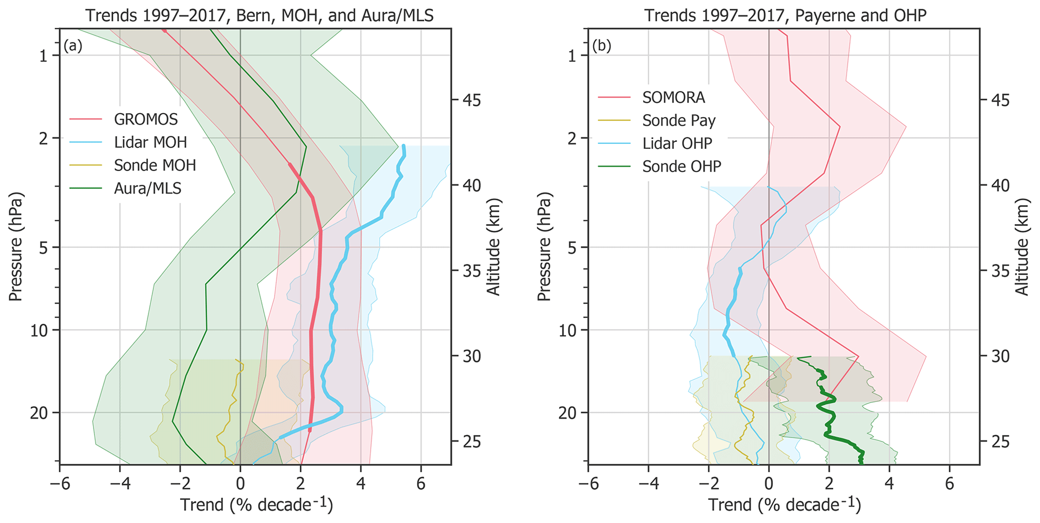
Figure 10Ozone trends of different ground-based instruments in central Europe and Aura/MLS (over Bern, Switzerland). The 2σ uncertainties are shown by shaded areas. Bold lines indicate trends that are significantly different from zero (at a 95 % confidence interval). The trends at Bern and MOH as well as the Aura/MLS trend are shown in (a), whereas (b) shows the trends from data sets at Payerne and OHP.
We observe that all instruments that measure in the upper stratosphere show a trend maximum between ∼ 4 and ∼ 1.8 hPa (between ∼ 37 and 43 km), which indicates that ozone is recovering at these altitudes. The trend maxima range from ∼ 1 % decade−1 to 3 % decade−1, which is comparable with recent, mainly satellite-based ozone trends for northern mid-latitudes (e.g. Ball et al., 2017; Frith et al., 2017; Sofieva et al., 2017; Steinbrecht et al., 2017; SPARC/IO3C/GAW, 2019). Only the lidar trend at MOH is larger throughout the whole stratosphere, with ∼ 3 % decade−1 in the middle stratosphere and 4 % decade−1 to 5 % decade−1 between 5 and 2 hPa. Nair et al. (2015) observed similar trend results for the MOH lidar, even if they consider 5 fewer years with a trend period ranging from 1997 to 2012. Steinbrecht et al. (2006) found that lidar data at MOH and OHP deviate from reference satellite data above 35 km before 2003, with less ozone at MOH and more ozone at OHP compared to SAGE satellite data (Stratospheric Aerosol and Gas Experiment; McCormick et al., 1989). Opposite drifts are reported by Eckert et al. (2014) after 2002 compared to MIPAS satellite data (Michelson Interferometer for Passive Atmospheric Sounding; Fischer et al., 2008). Combining those drifts might explain our large MOH trends and smaller OHP trends. The distance of ∼ 600 km between the MOH and OHP stations might also explain some differences between the lidar trends. Furthermore, our sampling results show that the lidar sampling at MOH leads to a larger trend in the lower stratosphere than using a continuous sampling, whereas OHP lidar sampling leads to a lower trend in the middle stratosphere. The large lidar trend at MOH and the comparable low OHP lidar trend might therefore also be partly explained by the sampling rate of the lidars. The GROMOS trend peaks at slightly lower altitudes than the trends of the other instruments. This difference might be related to the averaging kernels of GROMOS, which indicate that GROMOS retrieves information from higher altitudes than expected (∼ 2 km difference).
In the middle and lower stratosphere, at altitudes below 5 hPa (≈ 36 km), the estimated trends differ from each other. The microwave radiometers and the MOH lidar report trends of 0 % decade−1 to 3 % decade−1, and also the ozonesonde at OHP confirms this positive trend. However, the ozonesondes at MOH and Payerne as well as Aura/MLS and the OHP lidar report a trend of around 0 % decade−1 to −2 % decade−1 below 5 hPa. Some of these observed trend differences can be explained by instrumental changes or differences in processing algorithms and instrument setup. The discrepancy between ozonesonde and lidar trends at OHP, for example, are possibly due to the change of the pressure–temperature radiosonde manufacturer in 2007, which resulted in a step change in bias between ozonesonde and lidar observations. A thorough harmonization would be necessary to correct the trend for this change. The SOMORA trend shows a positive peak at 30 km, which is probably due to homogenization problems that are corrected in the new retrieval version of SOMORA, which is, however, not yet used in our analyses (Maillard Barras et al., 2019). Furthermore, we have shown that sampling rates and starting years have an important effect on the resulting trend. The trend period lengths differ between SOMORA, Aura/MLS, and the other data sets, which might also partly explain differences in trend estimates. To explain the remaining trend differences in the lower stratosphere, further corrections, e.g. for anomalies, instrumental changes, or sampling rates, would be necessary. In brief, trends in the lower stratosphere are not yet clear. For some instruments, significant positive trends are reported, but for many other instruments, trends are negative and mostly not significantly different from zero. This result reflects the currently ongoing discussion about lower stratospheric ozone trends (e.g. Ball et al., 2018; Chipperfield et al., 2018; Stone et al., 2018).
In summary, our ground-based instrument data agree that ozone is recovering around 3 hPa (≈ 39 km), with trends ranging between 1 % decade−1 and 3 % decade−1 for most data sets. In the lower and middle stratosphere between 24 and 37 km (≈ 31 and 4 hPa), however, the trends disagree, suggesting that further research is needed to explain the differences between ground-based trends in the lower stratosphere.
Our study emphasizes that natural or instrumental anomalies in a time series affect ground-based stratospheric ozone trends. We found that the ozone time series from the GROMOS radiometer (Bern, Switzerland) shows some unexplained anomalies. Accounting for these anomalies in the trend estimation can substantially improve the resulting trends. We further compared different ground-based ozone trend profiles and found an agreement on ozone recovery at around 40 km over central Europe. At the same time, we observed trend differences ranging between −2 % decade−1 and 3 % decade−1 at lower altitudes.
We compared the GROMOS time series with data from other ground-based instruments in central Europe and found that they generally agree within ±10 %. Periods with larger discrepancies have been identified and confirmed to be anomalies in the GROMOS time series. We did not find the origins of these anomalies and assume that they are due to instrumental issues of GROMOS. The identified anomalies have been considered in the GROMOS trend estimations because they can distort the trend. By testing this approach first on a theoretical time series and then with the real GROMOS data, we have shown that identifying anomalies in a time series and considering them in the trend analysis makes the resulting trend estimates more accurate. With this method, we propose an approach of advanced trend analysis based on the work of von Clarmann et al. (2010) that may also be applied to other ground- or satellite-based data sets to obtain more consistent trend results.
Comparing the GROMOS trend with other ground-based trends in central Europe suggests that ozone is recovering in the upper stratosphere between around 4 and 1.8 hPa (≈ 37 and 43 km). This result confirms recent, mainly satellite-based studies. At other altitudes, we have observed contrasting trend estimates. We have shown that the observed differences can partly be explained by different sampling rates and starting years. Other reasons might be instrumental changes or nonconformity in measurement techniques, instrumental systems, or processing approaches. Further, the spatial distance between some stations might explain some trend differences because different air masses can be measured, especially in winter when polar air extends over parts of Europe. Accounting for anomalies in the different data sets as proposed in the present study might be a first step to improve trend estimates. Combined with further corrections, e.g. for sampling rates or instrumental differences, this approach may help to decrease discrepancies between trend estimates from different instruments. In many other studies, the observed trend differences are less apparent because the ground-based data are averaged over latitudinal bands (e.g. WMO, 2014; Harris et al., 2015; Steinbrecht et al., 2017). Nevertheless, it is important to be aware that ground-based trend estimates differ considerably, especially in the lower stratosphere. Exploring the origin of the differences and improving the trend profiles in a similar way as we did for GROMOS may be an important further step on the way to monitoring the development of the ozone layer. To summarize, we have shown that anomalies in time series need to be considered when estimating trends. Our ground-based results confirm that ozone is recovering in the upper stratosphere above central Europe and emphasize the urgency to further investigate lower stratospheric ozone changes. The presented approach to improve trend estimates can help in this endeavour.
All ground-based data used in this study are available at ftp://ftp.cpc.ncep.noaa.gov/ndacc. The MLS data from the Aura satellite are available at https://disc.gsfc.nasa.gov/datasets/ML2O3_V004/summary (Schwartz, 2015).
LB and KH designed the concept and the methodology. LB carried out the analysis and prepared the manuscript. TvC provided the trend model. All co-authors contributed to the manuscript preparation and the interpretation of the results.
The authors declare that they have no competing interests. Thomas von Clarmann is co-editor of Atmospheric Chemistry and Physics, but he is not involved in the evaluation of this paper.
The authors thank the Aura/MLS team for providing the satellite data. This study has been funded by the Swiss National Science Foundation, grant number 200021-165516.
This paper was edited by Jens-Uwe Grooß and reviewed by two anonymous referees.
Bai, K., Chang, N.-B., Shi, R., Yu, H., and Gao, W.: An inter-comparison of multi-decadal observational and reanalysis data sets for global total ozone trends and variability analysis, J. Geophys. Res.-Atmos., 122, 1–21, https://doi.org/10.1002/2016JD025835, 2017. a
Ball, W. T., Alsing, J., Mortlock, D. J., Rozanov, E. V., Tummon, F., and Haigh, J. D.: Reconciling differences in stratospheric ozone composites, Atmos. Chem. Phys., 17, 12269–12302, https://doi.org/10.5194/acp-17-12269-2017, 2017. a, b, c
Ball, W. T., Alsing, J., Mortlock, D. J., Staehelin, J., Haigh, J. D., Peter, T., Tummon, F., Stübi, R., Stenke, A., Anderson, J., Bourassa, A., Davis, S. M., Degenstein, D., Frith, S. M., Froidevaux, L., Roth, C., Sofieva, V., Wang, R., Wild, J., Yu, P., Ziemke, J. R., and Rozanov, E. V.: Evidence for continuous decline in lower stratospheric ozone offsetting ozone layer recovery, Atmos. Chem. Phys., 18, 1379–1394, https://doi.org/10.5194/acp-18-1379-2018, 2018. a, b
Bates, B. C., Chandler, R. E., and Bowman, A. W.: Trend estimation and change point detection in individual climatic series using flexible regression methods, J. Geophys. Res.-Atmos., 117, 1–9, https://doi.org/10.1029/2011JD017077, 2012. a
Bourassa, A. E., Roth, C. Z., Zawada, D. J., Rieger, L. A., McLinden, C. A., and Degenstein, D. A.: Drift-corrected Odin-OSIRIS ozone product: Algorithm and updated stratospheric ozone trends, Atmos. Meas. Tech., 11, 489–498, https://doi.org/10.5194/amt-11-489-2018, 2018. a
Brewer, A. W. and Milford, J. R.: The Oxford-Kew Ozone Sonde, in: Proc. R. Soc. Lond. Ser. A, Mathematical and Physical Sciences, vol. 256, Royal Society, 470–495, http://www.jstor.org/stable/2413928 (last access: 28 March 2019), 1960. a
Calisesi, Y.: The stratospheric ozone monitoring radiometer SOMORA: NDSC application document, Research report no. 2003-11, Institute of Applied Physics, University of Bern, Switzerland, 2003. a
Calisesi, Y., Soebijanta, V. T., and van Oss, R.: Regridding of remote soundings: Formulation and application to ozone profile comparison, J. Geophys. Res., 110, D23306, https://doi.org/10.1029/2005JD006122, 2005. a
Chipperfield, M. P., Dhomse, S., Hossaini, R., Feng, W., Santee, M. L., Weber, M., Burrows, J. P., Wild, J. D., Loyola, D., and Coldewey-Egbers, M.: On the Cause of Recent Variations in Lower Stratospheric Ozone, Geophys. Res. Lett., 45, 5718–5726, https://doi.org/10.1029/2018GL078071, 2018. a, b
Chubachi, S.: A special ozone observation at Syowa station, Antarctica from February 1982 to January 1983, in: Atmos. Ozone, Proc. Quadrenn. Ozone Symp., edited by: Zerefos, C. S. and Ghazi, A., Halkidiki, Greece, 285–286, 1984. a
Connor, B. J., Parrish, A., and Tsou, J.-J.: Detection of stratospheric ozone trends by ground-based microwave observations, in: Proc. SPIE 1491, Remote Sens. Atmos. Chem., edited by: McElroy, James L. and McNeal, R. J., vol. 1491, International Society for Optics and Photonics, Orlando, FL, USA, 218–230, https://doi.org/10.1117/12.46665, 1991. a
Damadeo, R. P., Zawodny, J. M., Remsberg, E. E., and Walker, K. A.: The impact of nonuniform sampling on stratospheric ozone trends derived from occultation instruments, Atmos. Chem. Phys., 18, 535–554, https://doi.org/10.5194/acp-18-535-2018, 2018. a
Eckert, E., von Clarmann, T., Kiefer, M., Stiller, G. P., Lossow, S., Glatthor, N., Degenstein, D. A., Froidevaux, L., Godin-Beekmann, S., Leblanc, T., McDermid, S., Pastel, M., Steinbrecht, W., Swart, D. P. J., Walker, K. A., and Bernath, P. F.: Drift-corrected trends and periodic variations in MIPAS IMK/IAA ozone measurements, Atmos. Chem. Phys., 14, 2571–2589, https://doi.org/10.5194/acp-14-2571-2014, 2014. a, b
Eriksson, P., Jiménez, C., and Buehler, S. A.: Qpack, a general tool for instrument simulation and retrieval work, J. Quant. Spectrosc. Ra., 91, 47–64, https://doi.org/10.1016/j.jqsrt.2004.05.050, 2005. a
Eriksson, P., Buehler, S., Davis, C., Emde, C., and Lemke, O.: ARTS, the atmospheric radiative transfer simulator, version 2, J. Quant. Spectrosc. Ra., 112, 1551–1558, https://doi.org/10.1016/j.jqsrt.2011.03.001, 2011. a
Farman, J. C., Gardiner, B. G., and Shanklin, J. D.: Large losses of total ozone in Antarctica reveal seasonal ClOx∕NOx interaction, Nature, 315, 207–210, https://doi.org/10.1038/315207a0, 1985. a
Favaro, G., Jeannet, P., and Stübi, R.: Re-evaluation and trend analysis of the Payerne ozone soundings, Scientific report no. 63, MeteoSwiss, Zürich, Switzerland, 2002. a
Fischer, H., Birk, M., Blom, C., Carli, B., Carlotti, M., Von Clarmann, T., Delbouille, L., Dudhia, A., Ehhalt, D., Endemann, M., Flaud, J. M., Gessner, R., Kleinert, A., Koopman, R., Langen, J., López-Puertas, M., Mosner, P., Nett, H., Oelhaf, H., Perron, G., Remedios, J., Ridolfi, M., Stiller, G., and Zander, R.: MIPAS: An instrument for atmospheric and climate research, Atmos. Chem. Phys., 8, 2151–2188, https://doi.org/10.5194/acp-8-2151-2008, 2008. a
Frith, S. M., Stolarski, R. S., Kramarova, N. A., and McPeters, R. D.: Estimating uncertainties in the SBUV Version 8.6 merged profile ozone data set, Atmos. Chem. Phys., 17, 14695–14707, https://doi.org/10.5194/acp-17-14695-2017, 2017. a, b, c
Gaudel, A., Ancellet, G., and Godin-Beekmann, S.: Analysis of 20 years of tropospheric ozone vertical profiles by lidar and ECC at Observatoire de Haute Provence (OHP) at 44∘ N, 6.7∘ E, Atmos. Environ., 113, 78–89, https://doi.org/10.1016/j.atmosenv.2015.04.028, 2015. a
Godin, S., Mégie, G., and Pelon, J.: Systematic lidar measurements of the stratospheric ozone vertical distribution, Geophys. Res. Lett., 16, 547–550, 1989. a
Godin, S., Carswell, A. I., Donovan, D. P., Claude, H., Steinbrecht, W., McDermid, I. S., McGee, T. J., Gross, M. R., Nakane, H., Swart, D. P., Bergwerff, H. B., Uchino, O., von der Gathen, P., and Neuber, R.: Ozone differential absorption lidar algorithm intercomparison, Appl. Opt., 38, 6225–6236, https://doi.org/10.1364/AO.38.006225, 1999. a
Godin-Beekmann, S., Porteneuve, J., and Garnier, A.: Systematic DIAL lidar monitoring of the stratospheric ozone vertical distribution at Observatoire de Haute-Provence (43.92∘ N, 5.71∘ E), J. Environ. Monit., 5, 57–67, https://doi.org/10.1039/b205880d, 2003. a
Guirlet, M., Keckhut, P., Godin, S., and Mégie, G.: Description of the long-term ozone data series obtained from different instrumental techniques at a single location: The Observatoire de Haute-Provence (43.9∘ N, 5.7∘ E), Ann. Geophys., 18, 1325–1339, https://doi.org/10.1007/s00585-000-1325-y, 2000. a
Harris, N. R. P., Hudson, R., and Phillips, C.: SPARC/IOC/GAW, Assessment of trends in the vertical distribution of ozone, SPARC Report No. 1, WMO Ozone Research and Monitoring Project Report No. 43, Geneva, Switzerland, 1998. a, b
Harris, N. R. P., Hassler, B., Tummon, F., Bodeker, G. E., Hubert, D., Petropavlovskikh, I., Steinbrecht, W., Anderson, J., Bhartia, P. K., Boone, C. D., Bourassa, A., Davis, S. M., Degenstein, D., Delcloo, A., Frith, S. M., Froidevaux, L., Godin-Beekmann, S., Jones, N., Kurylo, M. J., Kyrölä, E., Laine, M., Leblanc, S. T., Lambert, J.-C., Liley, B., Mahieu, E., Maycock, A., de Mazière, M., Parrish, A. D., Querel, R., Rosenlof, K. H., Roth, C., Sioris, C., Staehelin, J., Stolarski, R. S., Stübi, R., Tamminen, J., Vigouroux, C., Walker, K. A., Wang, H. J., Wild, J., and Zawodny, J. M.: Past changes in the vertical distribution of ozone – Part 3: Analysis and interpretation of trends, Atmos. Chem. Phys., 15, 9965–9982, https://doi.org/10.5194/acp-15-9965-2015, 2015. a, b, c, d, e
Hatzaki, M., Flocas, H. A., Simmonds, I., Kouroutzoglou, J., Keay, K., and Rudeva, I.: Seasonal aspects of an objective climatology of anticyclones affecting the mediterranean, J. Clim., 27, 9272–9289, https://doi.org/10.1175/JCLI-D-14-00186.1, 2014. a
Hubert, D., Lambert, J.-C., Verhoelst, T., Granville, J., Keppens, A., Baray, J. L., Bourassa, A. E., Cortesi, U., Degenstein, D. A., Froidevaux, L., Godin-Beekmann, S., Hoppel, K. W., Johnson, B. J., Kyrölä, E., Leblanc, T., Lichtenberg, G., Marchand, M., McElroy, C. T., Murtagh, D., Nakane, H., Portafaix, T., Querel, R., Russell, J. M., Salvador, J., Smit, H. G. J., Stebel, K., Steinbrecht, W., Strawbridge, K. B., Stübi, R., Swart, D. P. J., Taha, G., Tarasick, D. W., Thompson, A. M., Urban, J., Van Gijsel, J. A. E., Van Malderen, R., Von Der Gathen, P., Walker, K. A., Wolfram, E., and Zawodny, J. M.: Ground-based assessment of the bias and long-term stability of 14 limb and occultation ozone profile data records, Atmos. Meas. Tech., 9, 2497–2534, https://doi.org/10.5194/amt-9-2497-2016, 2016. a, b
Hubert et al.: The temporal and spatial homogeneity of ozone profile data records obtained by ozonesonde, lidar and microwave radiometer networks, in preparation, 2019. a
Jeannet, P., Stübi, R., Levrat, G., Viatte, P., and Staehelin, J.: Ozone balloon soundings at Payerne (Switzerland): Reevaluation of the time series 1967–2002 and trend analysis, J. Geophys. Res.-Atmos., 112, D11302, https://doi.org/10.1029/2005JD006862, 2007. a
Jones, A., Urban, J., Murtagh, D. P., Sanchez, C., Walker, K. A., Livesey, N. J., Froidevaux, L., and Santee, M. L.: Analysis of HCl and ClO time series in the upper stratosphere using satellite data sets, Atmos. Chem. Phys., 11, 5321–5333, https://doi.org/10.5194/acp-11-5321-2011, 2011. a, b
Kämpfer, N.: Microwave remote sensing of the atmosphere in Switzerland, Opt. Eng., 34, 2413–2424, 1995. a
Keppens, A., Lambert, J. C., Granville, J., Miles, G., Siddans, R., Van Peet, J. C., Van Der A, R. J., Hubert, D., Verhoelst, T., Delcloo, A., Godin-Beekmann, S., Kivi, R., Stübi, R., and Zehner, C.: Round-robin evaluation of nadir ozone profile retrievals: Methodology and application to MetOp-A GOME-2, Atmos. Meas. Tech., 8, 2093–2120, https://doi.org/10.5194/amt-8-2093-2015, 2015. a
Komhyr, W. D.: Electrochemical concentration cells for gas analysis, Ann. Geophys., 25, 203–210, 1969. a
Kuttippurath, J. and Nair, P. J.: The signs of Antarctic ozone hole recovery, Sci. Rep., 7, 585 pp., https://doi.org/10.1038/s41598-017-00722-7, 2017. a
Maillard Barras, E., Ruffieux, D., and Hocke, K.: Stratospheric ozone profiles over Switzerland measured by SOMORA, ozonesonde and MLS/AURA satellite, Int. J. Remote Sens., 30, 4033–4041, https://doi.org/10.1080/01431160902821890, 2009. a
Maillard Barras, E., Haefele, A., Stübi, R., and Ruffieux, D.: A method to derive the Site Atmospheric State Best Estimate (SASBE) of ozone profiles from radiosonde and passive microwave data, Atmos. Meas. Tech. Discuss., 8, 3399–3422, https://doi.org/10.5194/amtd-8-3399-2015, 2015. a, b
Maillard Barras et al.: Trends of stratospheric ozone daily cycle, in preparation, 2019. a, b
McCormick, M., Zawodny, J., Veiga, R., Larsen, J., and Wang, P.: An overview of SAGE I and II ozone measurements, Planet. Space Sci., 37, 1567–1586, https://doi.org/10.1016/0032-0633(89)90146-3, 1989. a
Millán, L. F., Livesey, N. J., Santee, M. L., Neu, J. L., Manney, G. L., and Fuller, R. A.: Case studies of the impact of orbital sampling on stratospheric trend detection and derivation of tropical vertical velocities: solar occultation vs. limb emission sounding, Atmos. Chem. Phys., 16, 11521–11534, https://doi.org/10.5194/acp-16-11521-2016, 2016. a, b
Molina, M. J. and Rowland, F. S.: Stratospheric sink for chlorofluoromethanes: chlorine atom-catalysed destruction of ozone, Nature, 249, 810–812, https://doi.org/10.1038/249810a0, 1974. a
Moreira, L.: Trends and oscillations in middle atmospheric ozone observed by a ground-based microwave radiometer, Phd. thesis, University of Bern, Switzerland, 2017. a
Moreira, L., Hocke, K., Eckert, E., Von Clarmann, T., and Kämpfer, N.: Trend analysis of the 20-year time series of stratospheric ozone profiles observed by the GROMOS microwave radiometer at Bern, Atmos. Chem. Phys., 15, 10999–11009, https://doi.org/10.5194/acp-15-10999-2015, 2015. a, b, c, d, e
Moreira, L., Hocke, K., Navas-Guzmán, F., Eckert, E., von Clarmann, T., and Kämpfer, N.: The natural oscillations in stratospheric ozone observed by the GROMOS microwave radiometer at the NDACC station Bern, Atmos. Chem. Phys., 16, 10455–10467, https://doi.org/10.5194/acp-16-10455-2016, 2016. a, b
Moreira, L., Hocke, K., and Kämpfer, N.: Comparison of ozone profiles and influences from the tertiary ozone maximum in the night-to-day ratio above Switzerland, Atmos. Chem. Phys., 17, 10259–10268, https://doi.org/10.5194/acp-17-10259-2017, 2017. a
Nair, P. J., Godin-Beekmann, S., Pazmiño, A., Hauchecorne, A., Ancellet, G., Petropavlovskikh, I., Flynn, L. E., and Froidevaux, L.: Coherence of long-term stratospheric ozone vertical distribution time series used for the study of ozone recovery at a northern mid-latitude station, Atmos. Chem. Phys., 11, 4957–4975, https://doi.org/10.5194/acp-11-4957-2011, 2011. a, b
Nair, P. J., Godin-Beekmann, S., Froidevaux, L., Flynn, L. E., Zawodny, J. M., Russell, J. M., Pazmiño, A., Ancellet, G., Steinbrecht, W., Claude, H., Leblanc, T., McDermid, S., Van Gijsel, J. A. E., Johnson, B., Thomas, A., Hubert, D., Lambert, J.-C., Nakane, H., and Swart, D. P. J.: Relative drifts and stability of satellite and ground-based stratospheric ozone profiles at NDACC lidar stations, Atmos. Meas. Tech., 5, 1301–1318, https://doi.org/10.5194/amt-5-1301-2012, 2012. a
Nair, P. J., Godin-Beekmann, S., Kuttippurath, J., Ancellet, G., Goutail, F., Pazmiño, A., Froidevaux, L., Zawodny, J. M., Evans, R. D., Wang, H. J., Anderson, J., and Pastel, M.: Ozone trends derived from the total column and vertical profiles at a northern mid-latitude station, Atmos. Chem. Phys., 13, 10373–10384, https://doi.org/10.5194/acp-13-10373-2013, 2013. a
Nair, P. J., Froidevaux, L., Kuttippurath, J., Zawodny, J. M., Russell, J. M., Steinbrecht, W., Claude, H., Leblanc, T., Van Gijsel, J. A., Johnson, B., Swart, D. P., Thomas, A., Querel, R., Wang, R., and Anderson, J.: Subtropical and midlatitude ozone trends in the stratosphere: Implications for recovery, J. Geophys. Res.-Atmos., 120, 7247–7257, https://doi.org/10.1002/2014JD022371, 2015. a, b
National Research Council of Canada: Latest Solar Radio Flux Report from DRAO, Penticton, http://www.spaceweather.ca/solarflux/sx-4-en.php, last access: 12 March 2019. a
NDACC: Network for the Detection of Atmospheric Composition Change, http://www.ndaccdemo.org, last access: 12 March 2019. a
Newchurch, M. J., Yang, E.-S., Cunnold, D. M., Reinsel, G. C., Zawodny, J. M., and Russell, J. M.: Evidence for slowdown in stratospheric ozone loss: First stage of ozone recovery, J. Geophys. Res.-Atmos., 108, 4507, https://doi.org/10.1029/2003JD003471, 2003. a
Parkinson, C. L., Ward, A., and King, M. D. (Eds.): Earth Science Reference Handbook – A Guide to NASA's Earth Science Program and Earth Observing Satellite Missions, National Aeronautics and Space Administration, Washington, DC, 2006. a
Pazmiño, A., Godin-Beekmann, S., Hauchecorne, A., Claud, C., Khaykin, S., Goutail, F., Wolfram, E., Salvador, J., and Quel, E.: Multiple symptoms of total ozone recovery inside the Antarctic vortex during austral spring, Atmos. Chem. Phys., 18, 7557–7572, https://doi.org/10.5194/acp-18-7557-2018, 2018. a
Peter, R.: The Ground-based Millimeter-wave Ozone Spectrometer – GROMOS, Research report no. 97-13, Institute of Applied Physics, University of Bern, Switzerland, 1997. a
Ramaswamy, V., Chanin, M.-L., Angell, J., Barnett, J., Gaffen, D., Gelman, M., Keckhut, P., Koshelkov, Y., Labitzke, K., Lin, J.-J. R., O'Neill, A., Nash, J., Randel, W., Rood, R., Shine, K., Shiotani, M., and Swinbank, R.: Stratospheric temperature trends: Observations and model simulations, Rev. Geophys., 39, 71–122, https://doi.org/10.1029/1999RG000065, 2001. a
Reinsel, G. C., Miller, A. J., Weatherhead, E. C., Flynn, L. E., Nagatani, R. M., Tiao, G. C., and Wuebbles, D. J.: Trend analysis of total ozone data for turnaround and dynamical contributions, J. Geophys. Res.-Atmos., 110, D16306, https://doi.org/10.1029/2004JD004662, 2005. a
Rodgers, C. D.: Inverse Methods for Atmospheric Sounding: Theory and Practice, World Scientific Publishing Co. Pte. Ltd, Singapore, 2000. a, b
Rodgers, C. D. and Connor, B. J.: Intercomparison of remote sounding instruments, J. Geophys. Res., 108, 46–48, https://doi.org/10.1029/2002JD002299, 2003. a
Schanz, A., Hocke, K., and Kämpfer, N.: Daily ozone cycle in the stratosphere: Global, regional and seasonal behaviour modelled with the Whole Atmosphere Community Climate Model, Atmos. Chem. Phys., 14, 7645–7663, https://doi.org/10.5194/acp-14-7645-2014, 2014. a
Schotland, R. M.: Errors in the Lidar Measurement of Atmospheric Gases by Differential Absorption, J. Appl. Meteorol., 13, 71–77, https://doi.org/10.1175/1520-0450(1974)013<0071:EITLMO>2.0.CO;2, 1974. a
Schwartz, M., Froidevaux, L., Livesey, N. and Read, W.: MLS/Aura Level 2 Ozone (O3) Mixing Ratio V004, Greenbelt, MD, USA, Goddard Earth Sciences Data and Information Services Center (GES DISC), available at: https://disc.gsfc.nasa.gov/datasets/ML2O3_V004/summary (last accessed: 5 February 2018), 2015. a
Shepherd, T. G., Plummer, D. A., Scinocca, J. F., Hegglin, M. I., Fioletov, V. E., Reader, M. C., Remsberg, E., von Clarmann, T., and Wang, H. J.: Reconciliation of halogen-induced ozone loss with the total-column ozone record, Nat. Geosci., 7, 443–449, https://doi.org/10.1038/ngeo2155, 2014. a
Smit, H. G. J. and ASOPOS Panel: Quality Assurance and Quality Control for Ozonesonde Measurements in GAW, World Meteorological Organization, Global Atmosphere Watch, GAW Report No. 201, Geneva, Switzerland, 2013. a, b
Smit, H. G. J. and Kley, D.: Jülich Ozone Sonde Intercomparison Experiment (JOSIE), World Meteorological Organization, Global Atmosphere Watch, Report No. 130, 1996. a
Sofieva, V. F., Kyrölä, E., Laine, M., Tamminen, J., Degenstein, D., Bourassa, A., Roth, C., Zawada, D., Weber, M., Rozanov, A., Rahpoe, N., Stiller, G., Laeng, A., von Clarmann, T., Walker, K. A., Sheese, P., Hubert, D., van Roozendael, M., Zehner, C., Damadeo, R., Zawodny, J., Kramarova, N., and Bhartia, P. K.: Merged SAGE II, Ozone_cci and OMPS ozone profile dataset and evaluation of ozone trends in the stratosphere, Atmos. Chem. Phys., 17, 12533–12552, https://doi.org/10.5194/acp-17-12533-2017, 2017. a, b, c
Solomon, S., Ivy, D. J., Kinnison, D., Mills, M. J., Neely, R. R., and Schmidt, A.: Emergence of healing in the Antarctic ozone layer, Science, 353, 269–274, https://doi.org/10.1126/science.aae0061, 2016. a
SPARC/IO3C/GAW: SPARC/IO3C/GAW Report on Long-term Ozone Trends and Uncertainties in the Stratosphere, edited by: Petropavlovskikh, I., Godin-Beekmann, S., Hubert, D., Damadeo, R., Hassler, B., and Sofieva, V., SPARC Report No. 9, GAW Report No. 241, WCRP-17/2018, https://doi.org/10.17874/f899e57a20b, 2019. a, b, c, d, e, f, g
Steinbrecht, W., Claude, H., Schönenborn, F., McDermid, I. S., Leblanc, T., Godin, S., Song, T., Swart, D. P. J., Meijer, Y. J., Bodeker, G. E., Connor, B. J., Kämpfer, N., Hocke, K., Calisesi, Y., Schneider, N., de la Noë, J., Parrish, A. D., Boyd, I. S., Brühl, C., Steil, B., Giorgetta, M. A., Manzini, E., Thomason, L. W., Zawodny, J. M., McCormick, M. P., Russell, J. M., Bhartia, P. K., Stolarski, R. S., and Hollandsworth-Frith, S. M.: Long-term evolution of upper stratospheric ozone at selected stations of the Network for the Detection of Stratospheric Change (NDSC), J. Geophys. Res.-Atmos., 111, D10308, https://doi.org/10.1029/2005JD006454, 2006. a, b, c
Steinbrecht, W., Claude, H., Schönenborn, F., McDermid, I. S., Leblanc, T., Godin-Beekmann, S., Keckhut, P., Hauchecorne, A., Van Gijsel, J. A. E., Swart, D. P. J., Bodeker, G. E., Parrish, A. D., Boyd, I. S., Kämpfer, N., Hocke, K., Stolarski, R. S., Frith, S. M., Thomason, L. W., Remsberg, E. E., von Savigny, C., Rozanov, A., and Burrows, J. P.: Ozone and temperature trends in the upper stratosphere at five stations of the Network for the Detection of Atmospheric Composition Change, Int. J. Remote Sens., 30, 3875–3886, https://doi.org/10.1080/01431160902821841, 2009a. a, b, c
Steinbrecht, W., McGee, T. J., Twigg, L. W., Claude, H., Schönenborn, F., Sumnicht, G. K., and Silbert, D.: Intercomparison of stratospheric ozone and temperature profiles during the October 2005 Hohenpeißenberg Ozone Profiling Experiment (HOPE), Atmos. Meas. Tech., 2, 125–145, https://doi.org/10.5194/amt-2-125-2009, 2009b. a
Steinbrecht, W., Köhler, U., Schönenborn, F., Adelwart, M., Petersen, D., Heinen, M., Munier, H., Claude, H., Steiner, S., and Attmannspacher, W.: 50 Years of Routine Ozone Soundings at Hohenpeissenberg, Quadrennial Ozone Symposium of the International Ozone Commission, Edinburgh, UK, 4–9 September 2016, QOS2016-28-1, 2016. a, b
Steinbrecht, W., Froidevaux, L., Fuller, R., Wang, R., Anderson, J., Roth, C., Bourassa, A., Degenstein, D., Damadeo, R., Zawodny, J., Frith, S. M., McPeters, R., Bhartia, P., Wild, J., Long, C., Davis, S., Rosenlof, K., Sofieva, V., Walker, K., Rahpoe, N., Rozanov, A., Weber, M., Laeng, A., von Clarmann, T., Stiller, G., Kramarova, N., Godin-Beekmann, S., Leblanc, T., Querel, R., Swart, D., Boyd, I., Hocke, K., Kämpfer, N., Maillard Barras, E., Moreira, L., Nedoluha, G., Vigouroux, C., Blumenstock, T., Schneider, M., García, O., Jones, N., Mahieu, E., Smale, D., Kotkamp, M., Robinson, J., Petropavlovskikh, I., Harris, N., Hassler, B., Hubert, D., and Tummon, F.: An update on ozone profile trends for the period 2000 to 2016, Atmos. Chem. Phys., 17, 10675–10690, https://doi.org/10.5194/acp-17-10675-2017, 2017. a, b, c, d, e, f, g, h, i, j, k
Stiller, G. P., von Clarmann, T., Haenel, F., Funke, B., Glatthor, N., Grabowski, U., Kellmann, S., Kiefer, M., Linden, A., Lossow, S., and López-Puertas, M.: Observed temporal evolution of global mean age of stratospheric air for the 2002 to 2010 period, Atmos. Chem. Phys., 12, 3311–3331, https://doi.org/10.5194/acp-12-3311-2012, 2012. a, b
Stolarski, R. S. and Frith, S. M.: Search for evidence of trend slow-down in the long-term TOMS/SBUV total ozone data record: the importance of instrument drift uncertainty, Atmos. Chem. Phys., 6, 4057–4065, https://doi.org/10.5194/acp-6-4057-2006, 2006. a, b
Stone, K. A., Solomon, S., and Kinnison, D. E.: On the Identification of Ozone Recovery, Geophys. Res. Lett., 45, 5158–5165, https://doi.org/10.1029/2018GL077955, 2018. a, b
Strahan, S. E. and Douglass, A. R.: Decline in Antarctic Ozone Depletion and Lower Stratospheric Chlorine Determined From Aura Microwave Limb Sounder Observations, Geophys. Res. Lett., 45, 382–390, https://doi.org/10.1002/2017GL074830, 2018. a
Studer, S., Hocke, K., Schanz, A., Schmidt, H., and Kämpfer, N.: A climatology of the diurnal variations in stratospheric and mesospheric ozone over Bern, Switzerland, Atmos. Chem. Phys., 14, 5905–5919, https://doi.org/10.5194/acp-14-5905-2014, 2014. a
Tsou, J. J., Connor, B. J., Parrish, A. D., McDermid, I. S., and Chu, W. P.: Ground-based microwave monitoring of middle atmosphere ozone: Comparison to lidar and Stratospheric and Gas Experiment II satellite observations, J. Geol., 100, 3005–3016, 1995. a
von Clarmann, T., Grabowski, U., and Kiefer, M.: On the role of non-random errors in inverse problems in radiative transfer and other applications, J. Quant. Spectrosc. Ra., 71, 39–46, https://doi.org/10.1016/S0022-4073(01)00010-3, 2001. a, b
von Clarmann, T., Stiller, G. P., Grabowski, U., Eckert, E., and Orphal, J.: Technical note: Trend estimation from irregularly sampled, correlated data, Atmos. Chem. Phys., 10, 6737–6747, https://doi.org/10.5194/acp-10-6737-2010, 2010. a, b, c, d, e, f, g, h
Vyushin, D. I., Fioletov, V. E., and Shepherd, T. G.: Impact of long-range correlations on trend detection in total ozone, J. Geophys. Res., 112, D14307, https://doi.org/10.1029/2006JD008168, 2007. a, b
Wargan, K., Orbe, C., Pawson, S., Ziemke, J. R., Oman, L. D., Olsen, M. A., Coy, L., and Emma Knowland, K.: Recent Decline in Extratropical Lower Stratospheric Ozone Attributed to Circulation Changes, Geophys. Res. Lett., 45, 5166–5176, https://doi.org/10.1029/2018GL077406, 2018. a
Waters, J. W., Froidevaux, L., Harwood, R. S., Jarnot, R. F., Pickett, H. M., Read, W. G., Siegel, P. H., Cofield, R. E., Filipiak, M. J., Flower, D. A., Holden, J. R., Lau, G. K., Livesey, N. J., Manney, G. L., Pumphrey, H. C., Santee, M. L., Wu, D. L., Cuddy, D. T., Lay, R. R., Loo, M. S., Perun, V. S., Schwartz, M. J., Stek, P. C., Thurstans, R. P., Boyles, M. A., Chandra, K. M., Chavez, M. C., Chen, G. S., Chudasama, B. V., Dodge, R., Fuller, R. A., Girard, M. A., Jiang, J. H., Jiang, Y., Knosp, B. W., Labelle, R. C., Lam, J. C., Lee, K. A., Miller, D., Oswald, J. E., Patel, N. C., Pukala, D. M., Quintero, O., Scaff, D. M., Van Snyder, W., Tope, M. C., Wagner, P. A., and Walch, M. J.: The Earth Observing System Microwave Limb Sounder (EOS MLS) on the aura satellite, IEEE Trans. Geosci. Remote Sens., 44, 1075–1092, https://doi.org/10.1109/TGRS.2006.873771, 2006. a
Weatherhead, E. C., Reinsel, G. C., Tiao, G. C., Jackman, C. H., Bishop, L., Hollandsworth, S. M., Deluisi, J., Keller, T., Oltmans, S. J., Fleming, E. L., Wuebbles, D. J., Kerr, J. B., Miller, A. J., Herman, J., McPeters, R., Nagatani, R. M., and Frederick, J. E.: Detecting the recovery of total column ozone, J. Geophys. Res., 105, 22201–22210, https://doi.org/10.1029/2000JD900063, 2000. a
Weber, M., Coldewey-Egbers, M., Fioletov, V. E., Frith, S. M., Wild, J. D., Burrows, J. P., Long, C. S., and Loyola, D.: Total ozone trends from 1979 to 2016 derived from five merged observational datasets – the emergence into ozone recovery, Atmos. Chem. Phys., 18, 2097–2117, https://doi.org/10.5194/acp-18-2097-2018, 2018. a
Werner, J., Rothe, K. W., and Walther, H.: Monitoring of the stratospheric ozone layer by laser radar, Appl. Phys. B, 32, 113–118, https://doi.org/10.1007/BF00688815, 1983. a
WMO: Scientific Assessment of Ozone Depletion: 2014, World Meteorological Organization, Global Ozone Research and Monitoring Project – Report No. 55, Geneva, Switzerland, p. 416, 2014. a, b, c, d, e, f, g, h
WMO: Scientific Assessment of Ozone Depletion: 2018, World Meteorological Organization, Global Ozone Research and Monitoring Project – Report No. 58, Geneva, Switzerland, p. 588, 2018. a, b
Wolter, K. and Timlin, M. S.: Measuring the strength of ENSO events: How does 1997/98 rank?, Weather, 53, 315–324, https://doi.org/10.1002/j.1477-8696.1998.tb06408.x, 1998. a
Zanis, P., Maillard, E., Staehelin, J., Zerefos, C., Kosmidis, E., Tourpali, K., and Wohltmann, I.: On the turnaround of stratospheric ozone trends deduced from the reevaluated Umkehr record of Arosa, Switzerland, J. Geophys. Res.-Atmos., 111, D22307, https://doi.org/10.1029/2005JD006886, 2006. a