


Abstract
A main determinant of the habitability of exoplanets is the presence of stable liquid surface water. In an era of abundant possible targets, the potential to find a habitable world remains a driving force in prioritization. We present here a data-forward method to investigate the likelihood of a stable hydrosphere on the timescales of the formation of life, 1 Gyr, and beyond. As our primary application, we use this method to examine the potential hydrospheres of TESS objects of interest 700 d, 256 b (LHS 1140 b), and 203 b. We first present our selection criteria, which are based on an implementation of the Earth Similarity Index, as well as the results of an initial investigation into the desiccation of the targets, which reveals that TOI 203 b is almost certainly desiccated based on TESS observations. We then describe the characterization of the remaining targets and their host stars from 2MASS, Gaia, and TESS data and the derivation of sampled probability distributions for their parameters. Following this, we describe our process of simulating the desiccation of the targets' hydrospheres using the Virtual Planet Simulator, VPlanet, with inputs directly linked to the previously derived probability distributions. We find that 50.86% of the likely cases for TOI 700 d are desiccated, and no modeled cases for TOI 256 b are without water. In addition, we calculate the remaining water inventory for the targets, the percentage of cases that are continuing to lose water, and the rate at which these cases are losing water.
Export citation and abstract BibTeX RIS

Original content from this work may be used under the terms of the Creative Commons Attribution 4.0 licence. Any further distribution of this work must maintain attribution to the author(s) and the title of the work, journal citation and DOI.
1. Introduction
The launch of the Transiting Exoplanet Survey Satellite (TESS) has built upon the legacy of the Kepler missions, together discovering an astonishing number of exoplanets. This, along with the recently successful launch and commissioning of the James Webb Space Telescope (JWST), has made the potential discovery of a habitable planet outside of our solar system a more tangible goal.
Unfortunately, the current best chance of robustly assessing the habitability (i.e., stable liquid surface water) of a planet lies with JWST, which has significant limitations in both time available and resolution of atmospheric spectral signatures for smaller, potentially more Earth-like planets due to their small signal-to-noise ratio. As such, it is beneficial to prioritize future observations to those that are most likely to produce the most results using as few resources as possible.
Most current methods of prioritization lack proper treatment of the different potential states of the planetary systems they examine (i.e., orbital configuration and planetary composition). Instead, many study only one state or a few (e.g., Barnes et al. 2016; O'Malley-James & Kaltenegger 2017; Becker et al. 2020), often ignoring the effects of many potentially important parameters, especially mass, which is often poorly constrained in the absence of radial velocity measurements. A tantalizing option is a grid-based approach to fully capture the intricacies of the parameter space. However, this approach is slow and unwieldy, can easily ignore a number of likely states for the sake of speed, and, moreover, is devoid of likelihood information. Indeed, even the study by Fleming et al. (2020) uses preprescribed prior distributions instead of observational data. Estimating these parameter distributions severs the link between observations and simulations and requires careful consideration of covariances that are intrinsically captured and propagated in our method.
To this end, we have created a new end-to-end data-forward method of prioritization that is fast and flexible. We utilize Monte Carlo fitting of TESS light curves to fully analyze the effect of the potential distributions of parameters such as density and insolation on modeling the planets' orbital and atmospheric evolution. This allows us to robustly and thoroughly determine which have the highest chance of being habitable at the present day.
The method leaves room for additional constraints both theoretical and observational. However, we present a basic application using only TESS data and previously observed stellar parameters.
In this paper, we describe the selection process of our two targets, TESS objects of interest (TOIs) 256 b (LHS 1140 b) and 700 d, as well as the initial characterization of the targets and their host stars, in Section 2. Following this, Section 3 details the specifications for our coupled atmospheric and orbital evolution simulations using the modeling software package VPlanet (Barnes et al. 2020), as well as how these simulations are statistically linked to the TESS observations. In addition, we present four metrics to assess the degradation of a target planet's hydrosphere within the method. In Section 4, the results of the method are shown for both the initial light-curve characterization and the outcome of the simulations detailed in the previous section. Finally, Section 5 presents our conclusions and recommendations for future observations of both targets.
2. Initial Planet Selection and Characterization
Inferring meaningful statistics about the stability of liquid surface water and an Earth-like atmosphere requires accurate and complete parameter distributions for the planets' physical and orbital characteristics. In order to properly simulate these probability distributions, we begin from TESS's 2 minute cadence photometry data on the targets and perform an in-depth data reduction and fit the data using a Monte Carlo method. The resultant traces of each parameter are used in the desiccation simulations. This link between the data and simulations is detailed in Section 3. The reduction of each target pixel file (TPF) is handled separately for each sector observation. The resultant light curves are then merged and fit following the procedure in Section 2.3.
2.1. Target Selection
We implemented an adaptation of the Earth Similarity Index (ESI; Schulze-Makuch et al. 2011) to select the targets of interest. The ESI serves as a good basis for our purposes in this study by preferring Earth-like planets in terms of radius and insolation.
Instead of relying on one value for the ESI, however, we used the Markov Chain Monte Carlo (MCMC) sampler emcee (Foreman-Mackey et al. 2013) to estimate the likelihood that a target has an ESI of above 0.8. Input parameter distributions were obtained from the data validation files produced by the TESS Science Operations Pipeline (Jenkins et al. 2016) for all TOIs. The MCMC was sampled using 30 chains of 5000 steps each, resulting in 150,000 samples per parameter (Figure 1).
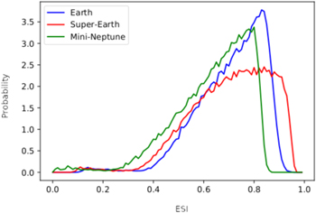
Figure 1. Probability of ESI values for TOI 256. The similarity to Earth (blue curve) is presented along with the similarity to a super-Earth (red curve) and a mini-Neptune (green curve) with Earth-like insolation.
Download figure:
Standard image High-resolution imageThe ESI of each TOI was calculated using the standard formulation except for using insolation in place of surface temperature. The inner threshold of insolation was set at the values determined by Leconte et al. (2015) to cause a runaway greenhouse effect, with the outer threshold being the CO2 maximum greenhouse needed to sustain liquid water (Kopparapu et al. 2014). The three TOIs presented in this study were the top targets for this selection criterion. Additional TOIs have since been discovered, but none have had a higher likelihood of being Earth-like.
Initial VPlanet simulations were performed on each planet by sampling the system parameters available from the Exoplanet Follow-up Observing Program (ExoFOP 2019), assuming a Gaussian distribution, and performing the method described in Section 3 for the primary atmosphere test. These initial simulations indicated that TOI 203 b was almost certainly desiccated; 99.08% of the models that started with 10 Earth oceans of water ended with no water. The simulations of TOI 700 d and 256 b, however, only returned 30.35% and 15.18% desiccated models, respectively. From these results, we decided to move forward in applying the process detailed herein to TOIs 700 d and 256 b only.
2.2. Host Star Parameterizations
The detection and characterization of transiting exoplanets begins with the host star, and inaccurate measurements of stellar properties have effects at every level of observation and modeling. In order to ensure that our targets are accurately modeled, we determine the host stars' radius, mean density, and effective temperature using standard methods in the analysis of M dwarfs (Berta-Thompson et al. 2015; Dittmann et al. 2017; Kostov et al. 2019; Ment et al. 2019) .
We acquire the measured K-band magnitude and parallax from the Two Micron All Sky Survey (2MASS; Skrutskie et al. 2006) and Gaia survey (Gaia Collaboration et al. 2016, 2018; Luri et al. 2018), respectively. The input parameters are assumed to be Gaussian, and the uncertainties on the output parameters are estimated with a simple Monte Carlo simulation using 200,000 samples from the input distributions. The necessary stellar parameters, as well as their estimated uncertainties, are included in Table 1.
Table 1. Model Inputs
| Parameter | Value | Source |
|---|---|---|
| TOI 256 | ||
| Host Star | ||
| KS (mag) | 8.821 ± 0.023 | 2MASS |
| VJ (mag) | 13.10 ± 0.01 | Gilbert et al. (2020) |
| Parallax (mas) | 66.829 ± 0.048 | Gaia DR2 |
| R* (R⊙) | 0.209 7 ± 0.00427 | This work |
| M* (M⊙) | 0.179 4 ± 0.00244 | This work |
| Teff (K) | 3200 ± 44 | This work |
| TOI 256 b | ||
| T0 (BJD − 2,457,000) | 1,399.93 ± 1 a | ExoFOP |
| ln(period) (days) | 3.208 ± 1 a | ExoFOP |
| ln(transit depth) (ppm) | 8.503 ± 0.055 | ExoFOP |
| TOI 256 c | ||
| T0 (BJD − 2,457,000) | 1,389.29 ± 1 a | ExoFOP |
| ln(period) (days) | 1.329 ± 1 a | ExoFOP |
| ln(transit depth) (ppm) | 7.832 ± 0.063 | ExoFOP |
| TOI 700 | ||
| Host Star | ||
| KS (mag) | 8.634 ± 0.022 | 2MASS |
| VJ (mag) | 14.18 ± 0.03 | Dittmann et al. (2017) |
| Parallax (mas) | 32.133 ± 0.027 | Gaia DR2 |
| R* (R⊙) | 0.440 3 ± 0.00937 | This work |
| M* (M⊙) | 0.463 4 ± 0.00464 | This work |
| Teff (K) | 3390 ± 44 | This work |
| TOI 700 b | ||
| T0(BJD − 2,457,000) | 1,490.98 ± 1 a | ExoFOP |
| ln(period) (days) | 2.300 ± 1 a | ExoFOP |
| ln(transit depth) (ppm) | 6.221 ± 0.095 | ExoFOP |
| TOI 700 c | ||
| T0(BJD − 2,457,000) | 1,548.75 ± 1 a | ExoFOP |
| ln(period) (days) | 2.776 ± 1 a | ExoFOP |
| ln(transit depth) (ppm) | 8.099 ± 0.073 | ExoFOP |
| TOI 700 d | ||
| T0(BJD − 2,457,000) | 1,742.15 ± 1 a | ExoFOP |
| ln(period) (days) | 3.622 ± 1 a | ExoFOP |
| ln(transit depth) (ppm) | 6.418 ± 0.073 | ExoFOP |
Note.
a Variance left at 1 to not overpredict values.Download table as: ASCIITypeset image
The mass of the stellar host is determined using the mass–luminosity relation from Benedict et al. (2016). This mass is then used to estimate the stellar radius using a relationship for single stars (Boyajian et al. 2012), and the mean density is calculated. We estimate the bolometric luminosity as the mean of the corrected K and V magnitudes (Mann et al. 2015, erratum, and Pecaut & Mamajek 2013, respectively) and calculate the effective temperature using the Stefan–Boltzmann law. Finally, we confirm these parameters using the Mann et al. (2019) K-magnitude luminosity-distance–mass relationship.
2.3. TESS Data Acquisition and Reduction
As with other studies using TESS data (e.g., Gilbert et al. 2020), we decided to apply a reduction scheme that differs from the standard pipeline. These changes consist of creating a custom photometry aperture for the files, applying reduction and decorrelation techniques while masking transits, and moving the Gaussian process (GP) fitting/removal to the data fitting portion. This process necessitates that we begin with the 2 minute cadence TPFs that have undergone an initial cleaning for cosmic rays and flagged observations.
We used the Python program lightkurve (Lightkurve Collaboration et al. 2018) to download the publicly available TPFs and created a custom aperture for each using the threshold method. This method selects pixels that have a flux higher than 3 standard deviations above the median brightness and are contiguous with the center pixel. Each aperture is visually inspected to ensure that it includes only the target star and is devoid of other contamination.
To avoid overcorrecting the data during transit, each TPF is then masked for the duration of each planet's transit(s) with room for error. Expected transit times and lengths, as well as the variance for each, are taken from ExoFOP and included in Table 1.
Using the pixel and time series masks, we perform a pixel-level decorrelation on each TPF using the built-in method in lightkurve. Finally, we extract each light curve from the TPFs, remove NANs and outliers >7σ outside of the expected transits, and normalize the light curves. An example of the final, cleaned light curve is given in Figure 2.

Figure 2. TESS light curve for TOI 256 cleaned for instrument systematics and normalized (upper panel) showing the GP model (green curve), the light curve minus the GP model (middle panel) showing the exoplanet transit model for planets b (blue curve) and c (orange curve), and the residual data with the GP and transit models subtracted (bottom panel).
Download figure:
Standard image High-resolution imageLight curves for each sector's observations are cleaned separately. The entire catalog of observations of TOI 256 was used, but only the first 11 sectors' observations were used for TOI 700 to be consistent with the data used in Gilbert et al. (2020) and Suissa et al. (2020).
Finally, the light curves are stitched together based on the average of the error in flux. The light curves for TOI 256 had similar errors and are stitched together before fitting. As TOI 700 has some differences in errors between sectors, the sectors were grouped together into four groups: sectors 1, 3, 4, and 5 form group 1; sectors 6 and 7 form group 2; sectors 8 and 9 form group 3; and sectors 10, 11, and 13 form group 4.
2.4. Light-curve Fitting and Analysis
The reduced and extracted light curves are fit for transits using the exoplanet and its dependencies (Foreman-Mackey et al. 2021; Salvatier et al. 2016; The Theano Development Team, Al-Rfou, R., Alain, G., et al 2016; Kumar et al. 2019; Astropy Collaboration et al. 2018; Luger et al. 2019; Foreman-Mackey et al. 2017). The stellar mass and radius are parameterized via a normal distribution bounded above zero. Limb-darkening parameters are estimated in-model following Kipping (2013a) and were sampled uniformly. The impact parameters were sampled uniformly between zero (the center of the star) and one plus the planet-to-star radius ratio for each planet (the edge of transit overlap). We used a beta distribution as a prior on the eccentricities, as suggested by Kipping (2013b), bounded between zero and one. The periastron angle was sampled randomly. Transit depths and periods were parameterized using their natural logs. All other system parameters are modeled using a Gaussian distribution.
The list of parameters included in the fit, as well as the values, is available in Table 1. Parameters described above that are not included in the table had random initial values. Variance for some parameters in the prior distributions is intentionally left high so as to not unduly influence the fitting procedure.
To model noise, we fit a GP that is a mixture of two simple harmonic oscillators comprised of two hyperparameters,  and
and  , as well as a mean flux offset, μF
, and the natural log of the variance,
, as well as a mean flux offset, μF
, and the natural log of the variance,  . The initial value for μF
is zero, and
. The initial value for μF
is zero, and  is calculated from the variance of the flux with transits masked. The initial value for
  is set to be
  , and
, and  is initially zero. The variance for the noise parameters is set at 10 for each value to allow adequate flexibility in the modeling process.
We first run the parameters through the version of the PyMC3 (Salvatier et al. 2016) optimization routine that was made for use with exoplanet. The initial transit light curves for each planet are plotted along with the GP model and residual (Figure 2) and visually inspected to confirm that the model transits line up with the observed light curve. In addition, the optimization solution is inspected for significant deviations from the expected parameters, as this can indicate that the model is incorrect and must be changed. In practice, changes are made if the median values differ from the expected by more than a standard deviation, the errors are abnormally large, or the model chains do not converge.
After the initial model is inspected, a mask is created for data outside 5σ of the residual mean. This secondary data clipping enables more accuracy in the GP modeling, resulting in a more accurate light-curve fit.
The resulting light curve is used in a second optimization of the parameters that yields a final model to be sampled using the No U-turn Sampler (Hoffman & Gelman 2011). We use four chains with 6000 tuning steps and 5000 draw steps each, yielding a trace of 20,000 steps total. For all traces, the Gelman–Rubin diagnostic (Gelman & Rubin 1992) was near 1.0, and the number of effective samples was over 1000 for all parameters. The sampled traces are saved as fits files and available upon request. Section 4 shows the deterministic parameters computed as part of this sampling, as well as their median and variance.
3. Desiccation Simulations
A major concern of exoplanet habitability is the ability to sustain liquid water at the surface long enough for life to have the chance to form, especially around smaller (i.e., M dwarf) stars (Luger & Barnes 2014). These smaller stars tend to actively flare well into their lives, spewing dangerous amounts of X-ray and ultraviolet (XUV) radiation that can destroy water and lead to the total desiccation of their satellites (Reid & Hawley 2005; Scalo et al. 2007).
On Earth, our one data point for life, the period between the formation of the oceans and the initial stage of life is estimated to be at most 770 Myr and as little as 260 Myr (Dodd et al. 2017). Because of the activity level of M dwarf stars, however, we will investigate whether or not the hydrosphere is stable up to 1 Gyr after the system forms. Though we cannot say for certain if life has or will evolve on the targets, this time period samples Earth-like timescales for life evolution while allowing for the greater activity likely around M dwarfs.
For each parameter set in the trace obtained by the methods in Section 2, we instantiate and execute two VPlanet simulations of orbital, rotational, and atmospheric evolution using the stellar, atmesc, and eqtide modules. The first of the two simulations assumes the planet formed roughly 1 Myr after the star and integrates until 1 Gyr. This choice is made to line up with the lower limit of predicted protoplanetary disk lifetimes of 1–10 Myr (Walter et al. 1988; Strom et al. 1989). This is intentionally before the lower limits on theoretical predictions of the in situ formation of our solar system's terrestrial planets (Chambers 2004; Kleine et al. 2009; Raymond et al. 2014) to allow for more erosion of the hydrosphere over the course of the simulations, producing a more conservative result. The second simulation takes the system environment as it has been recently observed and models the next gigayear. Both simulations address the issue of hydrosphere stability, focusing on primary and secondary atmospheres, respectively.
3.1. VPlanet Setup and Assumptions
Before setting up the input files, we estimate the planet mass using the nonparametric method from Ning et al. (2018). We use the mrexo package for python (Kanodia et al. 2019) with the option to generate a complimentary MCMC trace for a posterior sample of the target planets' radii (Figure 3). A practical example can be seen in Figure 4 for TOI 256 b. This naive approximation can be replaced with the resultant probability distribution from simultaneously fitting transit and radial velocity measurements for more accurate simulations. We instead utilize this naive approach to highlight the potential insights gained from photometric transit data alone.
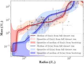
Figure 3. Figure adapted from Kanodia et al. (2019) highlighting the nonparametric fit for the mass given the radius used in this work shown in red. The accompanying fit for the radius given the mass is also shown in blue. The mean of the fits is shown as a dark line, and the shaded regions show the 16% and 84% quantiles for the conditional distributions. The data used in this fitting are from the Kepler data set.
Download figure:
Standard image High-resolution image
Figure 4. Log radius (top left panel) from the TESS data fitting, log mass given this radius distribution (bottom right panel), and their 2D probability distribution (bottom left panel) showing the bimodality of the mass fitting.
Download figure:
Standard image High-resolution imageThe atmesc model uses a simple, energy-limited atmospheric escape model (Watson et al. 1981) based on investigations of the solar wind by Parker (1964),

where  is the XUV energy flux, Mp
is the mass of the planet, Rp
is the planet radius,
is the XUV energy flux, Mp
is the mass of the planet, Rp
is the planet radius,  XUV ≈ 0.1 is the initial XUV absorption efficiency, and Ktide is a tidal correction term of order unity (Erkaev et al. 2007). This model is an inferred trend in atmospheric escape as a function of planet size and irradiation based on statistical studies of all known exoplanets (Owen & Wu 2013; Lopez & Rice 2018). It is applied to these targets as an estimate in the absence of specific knowledge of their individual atmospheric escape processes, especially over such a large mass range. We allow XUV to vary over the lifetime of the star as in Bolmont et al. (2016). This quantity is integrated over the planet's effective radius to incoming XUV energy,

(Lehmer & Catling 2017), where H is the atmospheric scale height, pXUV is the pressure at the effective XUV absorption level, and ps is the pressure at the surface.
As fluctuation in the stellar luminosity can greatly affect the model output, we chose to use the accepted values of 0.0233 L⊙ for TOI 700 and 0.00441 L⊙ for TOI 256 instead of the trace values. The current stellar age is also taken to be the accepted values of 1.5 and 5 Gyr, respectively. The radius and mass (and thus the density) are fixed to the average values of the trace. The stellar module interpolates over the mass and time of the Baraffe et al. (2015) evolutionary tracks, and the XUV luminosity is tracked using the broken power-law model of Ribas et al. (2005):

As is standard in these simulations for M dwarf–type stars, we use fsat = 1e − 3 for the saturation phase ratio, τ = 1 Gyr, and βXUV = −1.23 for the power-law exponent, which is, in this case, set for Sun-like (smaller) stars (Ribas et al. 2005).
We assume that the planet has no hydrogen/helium envelope, as this is eroded in the model before water loss begins. In this case, the model assumes that atmospheric escape only takes place if the planet enters the runaway greenhouse threshold (Kopparapu et al. 2013). In this case, the surface temperature exceeds 647 K, fully evaporating surface oceans and leading to a water vapor–dominated upper atmosphere (e.g., Kasting 1988).
Efficient oxygen sinks are turned on in the model we use. This instantly removes photolytically produced oxygen from the atmosphere, preventing it from building up. This raises the threshold for the diffusion-limited flux of oxygen atoms through the background atmosphere of hydrogen,

which is the limit above which the model adjusts the energy-limited flux equation as follows:

where mc is the crossover mass, the largest particle mass that can be dragged through the outflow:
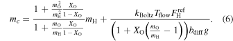
In the equations above, mH is the mass of the hydrogen atoms, mO is the mass of the oxygen atoms, kBoltz is the Boltzmann constant, Tflow = 400 K is the temperature of the hydrodynamic flow (Hunten et al. 1987; Chassefière 1996),  is the binary diffusion ratio for the two species (Zahnle & Kasting 1986), g is the planet's acceleration due to gravity, and XO is the molar mixing ratio of oxygen at the base of the flow.
This model for determining hydrosphere degradation is a very approximate description and neglects to include many key factors in the loss of an atmosphere, such as the wavelength-dependent nature of heating the upper atmosphere and any nonthermal escape processes (e.g., flares). In addition, other photochemical and 3D hydrodynamic processes within the atmosphere can alter the rate of outflow. However, several statistical studies have shown that the escape rate scales with the stellar XUV flux and inversely with the gravitational potential energy of the gas (e.g., Lopez et al. 2012; Lammer et al. 2013; Lopez & Rice 2018; Owen & Wu 2013, 2017). The uncertainties regarding physics and the specifics of each planet are folded into the XUV escape efficiency XUV ≈ 0.1, which has predicted the correct escape fluxes within a reasonable margin in these studies. The lack of specific information necessary to accurately model hydrodynamic escape necessitates the use of this kind of model for the purposes of our method, which aims to prioritize targets for follow-up observations to obtain this information.
In order to simulate the hydrosphere degradation during the active phase of the star, we assign the initial water on the simulated planet to be 10 Earth oceans as in Luger & Barnes (2014) for their most water-rich case. As we lack planetary formation and migration information of the target systems, their initial water inventory is difficult to ascertain. However, Earth is thought to have formed and accreted up to 70 oceans worth of water (Morbidelli et al. 2000; Raymond et al. 2006; Chassefière et al. 2012), making this a conservative estimate for initial water inventory.
The stability of a secondary hydrosphere is tested by setting the initial water inventory in Earth oceans to be proportional to the planet's mass in Earth masses. This tests the possibility that the planets can currently support a proportional amount of stable water for a long time and thus retain any primary or secondary hydrosphere for long enough that life could develop. Neither method is intended to be a definitive judgment of the planets' habitability.
The simulation results are given in Section 4. For statistics relating to TOI 700 d, the parameters are weighted according to the number of data points in their respective light curves. The output and aggregate files of the final parameters are available upon request.
3.2. Desiccation Metrics
We use four desiccation metrics to analyze the VPlanet outputs: desiccation percentage, remaining water inventory, percent of static models, and nonstatic desiccation rate. The necessary components of each metric are calculated during the data aggregation phase along with the results presented in Section 4.
3.2.1. Desiccation Percentage
This metric is simply calculated by dividing the number of simulations that become completely desiccated by the total number of simulations. As the uncertainty relating to the fitted parameters could be relatively large, this metric gives a simple first glance at the sustainability of the hydrosphere across the parameter space. Desiccation percentage is mostly applicable to primary hydrosphere degradation, as this is when the bulk of the water is lost in the simulations.
3.2.2. Remaining Water Inventory
The remaining water inventory is calculated from the water mass of the final time step in the simulation. For the set of simulations starting with 10 Earth oceans of water, the metric is taken to be this final value. This is instead expressed as a percentage of the original water mass for the secondary simulations with proportional initial water.
Two versions of this metric are presented here: one that includes desiccated cases and one that does not. Including desiccated cases essentially yields a reflection of the desiccation percentage metric, while rejecting desiccated cases explores not only the final water distribution in hydrated cases but, more importantly, what the expected amount of water is given that water is discovered on the target.
3.2.3. Static Cases
The static case percentage tracks how many of the final model states have ceased losing water. As desiccated models would inherently be static, they are excluded. To calculate the metric, the difference of water present in the final two steps of nondesiccated models is taken and counted if it is zero. After the aggregation is finished, the final count of static cases is divided by the number of nondesiccated models to form the metric. This reveals the stability of the planets' overall hydrosphere, should one exist, which is important for determining longer-term sustainability.
3.2.4. Nonstatic Desiccation Rate
Finally, for those models that are losing water, we take a derivative 1 Myr from the stop time to determine the final desiccation rate. This is a fairly selective metric, as in both systems, the majority of cases were static; however, in more active systems, this metric is important to determine the likelihood of complete desiccation at the present time.
4. Results
4.1. System Parameters
In this section, we present the deterministic parameters computed by sampling the resultant trace of fitting TESS light curves for TOIs 700 and 256, as well as their median and variance. In addition, the naive mass prediction for each planet is given.
The TOIs 700 d and 256 b have posterior predicted periods of  and
and  days and posterior predicted radii of
  and
and  R⊕, respectively. The results of the fit are well in line with other studies using TESS data (Gilbert et al. 2020; Lillo-Box et al. 2020; ExoFOP 2019). Gilbert et al. (2020) and Lillo-Box et al. (2020) used other observations to model stellar variability from the All-Sky Automated Survey for Supernovae and HARPS + ESPRESSO, respectively, leading to small discrepancies between their studies and this work.
From radial velocity observations, the mass of TOI 256 b is known to be M256b = 6.48 ± 0.46 M⊕ (Lillo-Box et al. 2020), well within the standard error on our naive prediction, presented in Table 2, which also considers the potential for the target to be gaseous. The effect of the bimodal mass predictions is evident in Figures 5 and 6, where the predicted density has a degeneracy with the predicted water loss. The values given here and used in the simulations serve as examples for the use of this method when radial velocity measurements are not available.

Figure 5. Remaining water mass (top left panel), natural log of the predicted density (bottom right panel), and their 2D probability distribution (bottom left) for TOI 256 b. The data are split into higher (pink) and lower (blue) densities for all panels using the density of Mars (horizontal line in bottom left panel) as the dividing factor. The increase in water retention below the density division is due to the implied presence of an extended gaseous envelope. As the observed natural log density of TOI 256 b is approximately 8.96 (Lillo-Box et al. 2020), we predict that it will retain most of its initial water inventory.
Download figure:
Standard image High-resolution image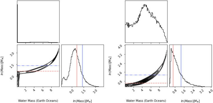
Figure 6. Both corner plots highlight the remaining water mass (top left panel), natural log of the predicted mass (bottom right panel), and their 2D probability distribution (bottom left panel) for TOI 700 d. The predicted mass using the density of Mars is shown by the pink line, and the predicted mass using the mass–radius relationship of Sotin et al. (2007) is shown by the blue line. The left set of panels includes fully desiccated models, whereas the right set is constructed from models that retain some water. If the planet is of a terrestrial density (i.e., as predicted by Sotin et al. 2007), then we expect that it will lose little of its primordial water while in the runaway greenhouse phase of evolution.
Download figure:
Standard image High-resolution imageTable 2. Derived Planet Parameters
| Parameter | Median | −1σ | +1σ |
|---|---|---|---|
| TOI 256 | |||
| TOI 256 b | |||
| Period (days) | 24.737 | 6.1e − 5 | 6.3e − 5 |
| Radius (R⊕) | 1.650 | 0.078 | 0.087 |
| T0(BJD − 2,457,000) | 1,399.929 | 0.001 | 0.001 |
| Impact parameter | 0.269 | 0.188 | 0.232 |
| ln(depth) (ppm) | 8.806 | 0.053 | 0.052 |
| Mass M⊕ | 2.320 | 1.822 | 5.221 |
| Mass (from log; M⊕) | 2.847 | 1.746 | 4.928 |
| TOI 256 c | |||
| Period (days) | 3.778 | 6e − 6 | 6.1e − 6 |
| Radius (R⊕) | 1.155 | 0.057 | 0.063 |
| T0(BJD − 2,457,000) | 1,389.293 | 0.001 | 0.001 |
| Impact parameter | 0.237 | 0.173 | 0.267 |
| ln(depth) (ppm) | 8.103 | 0.055 | 0.054 |
| Mass M⊕ | 1.103 | 0.700 | 1.445 |
| Mass (from log; M⊕) | 1.413 | 0.636 | 1.371 |
| TOI 700 | |||
| TOI 700 b | |||
| Period (days) | 9.977 | 0.003 | 0.019 |
| Radius (R⊕) | 0.980 | 0.090 | 0.091 |
| T0(BJD − 2,457,000) | 1,331.263 | 0.065 | 0.075 |
| Impact parameter | 0.242 | 0.176 | 0.262 |
| ln(depth) (ppm) | 6.276 | 0.140 | 0.136 |
| Mass M⊕ | 0.840 | 0.577 | 1.257 |
| Mass (from log; M⊕) | 1.206 | 0.733 | 1.199 |
| TOI 700 c | |||
| Period (days) | 16.045 | 0.006 | 0.005 |
| Radius (R⊕) | 2.975 | 0.185 | 0.271 |
| T0(BJD − 2,457,000) | 1,339.991 | 0.084 | 0.072 |
| Impact parameter | 0.908 | 0.020 | 0.018 |
| ln(depth) (ppm) | 8.061 | 0.047 | 0.050 |
| Mass M⊕ | 5.377 | 4.392 | 12.072 |
| Mass (from log; M⊕) | 7.480 | 4.043 | 11.273 |
| TOI 700 d | |||
| Period (days) | 37.406 | 0.062 | 0.068 |
| Radius (R⊕) | 1.123 | 0.114 | 0.131 |
| T0(BJD − 2,457,000) | 1,330.401 | 0.560 | 0.485 |
| Impact parameter | 0.424 | 0.278 | 0.233 |
| ln(depth) (ppm) | 6.501 | 0.166 | 0.167 |
| Mass M⊕ | 0.922 | 0.660 | 1.575 |
| Mass (from log; M⊕) | 1.404 | 0.681 | 1.492 |
Download table as: ASCIITypeset image
4.2. Desiccation Metrics
We present the desiccation metrics for TOIs 700 d and 256 b in Table 3 and the correlation between water loss and density in Figures 5 and 6. In many cases, both targets appear to be able to maintain a stable hydrosphere, which is a strong predictor for their habitability; all cases with terrestrial densities retain some water.
Table 3. Desiccation Metrics
| Metric | Median | −1σ | +1σ |
|---|---|---|---|
| TOI 256 b | |||
| Desiccation | 0% | ⋯ | ⋯ |
| Remaining water inventory (Earth oceans) | 6.733 | 0.622 | 1.138 |
| Nondesiccated inventory (Earth oceans) | ⋯ | ⋯ | ⋯ |
| Final static | 100% | ⋯ | ⋯ |
| Desiccation rate (Earth oceans Gyr–1) | ⋯ | ⋯ | ⋯ |
| TOI 700 d | |||
| Desiccation | 50.8% | ⋯ | ⋯ |
| Remaining water inventory (Earth oceans) | 0 | 0 | 5.811 |
| Nondesiccated inventory (Earth oceans) | 4.694 | 2.719 | 2.531 |
| Final static | 63.1% | ⋯ | ⋯ |
| Desiccation rate (Earth oceans Gyr–1) | 2.602 | 0.805 | 1.600 |
Download table as: ASCIITypeset image
For all planets in the target systems, modern simulations using proportional water inventories resulted in no water loss. This is due in majority to the low activity levels of the host stars, resulting in low XUV flux that did not trigger runaway greenhouse effects and thus water loss in the model. Thus, these results are not presented in Table 3. Unfortunately, no other planet besides the two targets shown in Table 3 had more than 1% of their simulations conclude with remaining water. In addition, of those that retained water, none had any static cases, meaning their hydrospheres would be predicted to degrade until fully desiccated. They are excluded from the table for this reason.
Desiccated models are included when calculating the remaining water inventory statistics, resulting in a peak in the distribution at zero. Because of this, the desiccation percent is a more useful metric for assessing the stability of a primary/formation hydrosphere. As expected, the planets that are safely in the habitable zone have the fewest desiccated cases and retain the most water.
4.2.1. TOI 700 d
As just over 50% of models for TOI 700 d returned a desiccated state, the median value of the remaining water mass is zero Earth oceans. For this reason, we also present this metric without desiccated values to examine the distribution of the remaining water mass should the planet retain water. This resulted in  Earth oceans remaining. We find that for TOI 700 d and smaller planets, this nonzero value is more appropriate to consider, as the prospective mass of the desiccated cases is inconsistent with the reasonable density for a rocky planet.
4.2.2. TOI 256 b
All simulations of TOI 256 b returned no desiccated models with  Earth oceans of water remaining. As this planet has a mass consistent with a rocky planet (Dittmann et al. 2017; Lillo-Box et al. 2020), these simulations indicate that TOI 256 b could likely have a large ocean covering most if not all of the surface, as has been previously predicted (e.g., Lillo-Box et al. 2020).
4.3. Discussion
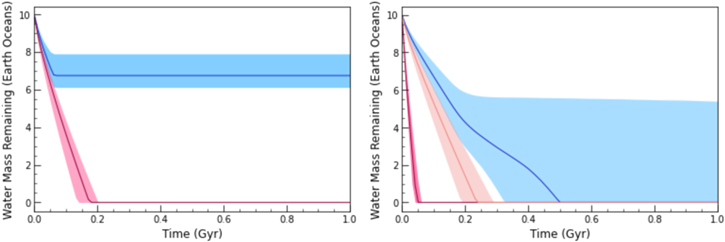
As the model for water loss is an approximation, and many other factors that influence the hydrodynamic outflow of a planet's hydrosphere have been neglected, the results of this study are no final judgment of a target's habitability. In addition, further and significant loss of water has been shown to occur in a nitrogen-poor Earth atmosphere following the early runaway greenhouse period (Wordsworth & Pierrehumbert 2013). Figure 7 clearly shows this, as the models cease losing water the moment the early runaway greenhouse period ends.
Figure 7. Water loss over time for all planets in the TOI 256 (left panel) and 700 (right panel) systems. On the left, TOI 256 b is shown in blue, and 256 c is shown in red. On the right, planet 700 b is shown in red, 700 c is shown in peach, and 700 d is shown in blue. As water loss in the model is tied to the runaway greenhouse phase, models that deviate from this phase early lose less water. As shown in other figures and in the model description, this strongly correlates with the predicted mass of the planet.
Download figure:
Standard image High-resolution image
To combat these factors, we made an effort to induce a more conservative modeling procedure by turning on efficient oxygen sinks, beginning the model at t = 1 Myr, and removing any initial hydrogen envelope that might shield the water from XUV radiation. However, the results conveyed are likely accurate within a few factors and constitute a sufficiently robust prediction of water retention on the targets to inform follow-up observations that might shed further light on their specific scenarios.
4.3.1. Comparison with Initial Simulations
In Section 2.1, we outlined preliminary simulations using VPlanet and an MCMC method using static distributions as opposed to simulations completed using the MCMC trace from directly fitting TESS data.
These initial simulations differ significantly in terms of desiccation rates compared to the new method outlined in this work. Object TOI 700 d increased the number of desiccated models by around 20%, whereas TOI 256 b decreased from around 15% to no desiccated models. These differences and the discrepancies between the two targets are due to the new method detailed herein, which more accurately treats the potential parameter distributions and inherently accounts for cross-correlations between parameters.
4.3.2. Mass Dependence for Rocky Bodies
Figure 5 illustrates the dependence of water retention on the mass of the planet for TOI 700 d. At masses lower than the median predicted mass in log space, 1.4 M⊕, the planet is certainly desiccated, but at masses indicating a terrestrial density, the planet only loses a maximum of eight Earth oceans of water. As expected, more massive planets retain more water, as their surface gravity is higher. The example of TOI 700 d clearly shows the necessity of thorough radial velocity measurements of smaller exoplanets, as density, and thus mass, are such strong predictors of hydrosphere stability.
4.3.3. Density Dependence for Intermediate Bodies
Figure 6 presents the desiccation of TOI 256 b against the predicted density used in the model. This is similar to the previous figure, but as this planet's radius is in the Fulton Gap (Fulton et al. 2017), a naive mass approximation gives a relatively equal probability of it being rocky or gaseous. The density of Mars is used as a dividing line, highlighting the differences between these types of planets.
For rocky planets of this size, the curve follows much the same curve as TOI 700 d. As the density and thus the mass lowers, the planet is unable to retain the photodissociated water and becomes desiccated. However, for gaseous planets, the amount of water retained increases with decreasing density for a portion of the distribution. This is due to the implied presence of an extended gaseous envelope that both protects the lower atmospheric water from disassociation and prevents hydrogen and oxygen from outflowing effectively. Similarly to the previous target, the case of TOI 256 b highlights the usefulness of radial velocity measurements in determining the potential habitability of an exoplanet.
4.3.4. Comparison of TOI 700 d to Other Studies
Suissa et al. (2020) explored 20 possible climate scenarios for TOI 700 d using the ExoCAM modeling package. Of these scenarios, the most likely ones given the work in our study are aqua planets in synchronous orbits. As we predict the loss of a significant amount of water, this correlates with the buildup of a relatively large amount of O2 on the planet's surface (Luger & Barnes 2014). As these simulations do not include a photochemical model, they neglect this significant factor. Because of this, more simulations including photochemical modeling must be conducted to predict the potential atmospheric states more accurately.
4.3.5. Future Observation Recommendations
Unfortunately, TOI 700 will not be observed by JWST in its Cycle 1 observations, potentially due to its small size and thus signal-to-noise ratio. Hopefully, the potential existence of a fourth planet in the system will lead to TOI 700 becoming a higher-priority system. Radial velocity measurements of TOI 700 d would greatly aid in further characterization of the planet and give a foundation for the planning of atmospheric observations with JWST.
Water on TOI 256 b was tentatively discovered using the Hubble Space Telescope's WFC3 (Edwards et al. 2020). This, along with radial velocity observations using ESPRESSO (Lillo-Box et al. 2020), strongly implies the existence of a large surface ocean on the planet, which is consistent with our findings that TOI 256 b should lose little, if any, of its primordial and accumulated water. Observations of TOI 256 b in Cycle 1 of JWST are aimed at confidently identifying water and other volatiles present in the atmosphere of the planet.
5. Conclusions
We have analyzed two high-priority TESS planets, TOIs 256 b and 700 d, for their potential to retain a stable hydrosphere using a new, flexible method that incorporates observational data, as opposed to other methods that use assumed parameter distributions. Preserving the correlations inherent in data fitting procedures, such as between the fitted radius and mass predictions, is an important step in assessing the habitability of exoplanets and deciding which, if any, future observations are needed for further refinement.
We applied the method to two highly prioritized TESS-observed planets, TOIs 256 b (LHS 1140 b) and 700 d, and assessed the likelihood that they retain stable hydrospheres to the present day through several metrics. Even with conservative initial water inventories, both planets retain water in a significant number of modeled cases (100% and 49%, respectively). In addition, both planets are highly likely to retain a significant amount of water if they are predominantly rocky.
Further observations of both planets are upcoming priorities, with TOI 256 b to be observed by the recently launched and commissioned JWST in its first cycle. The characterization of this planet's atmosphere will enable more precise simulations of other planets in the future, refining the procedures for identifying and prioritizing potentially habitable planets.
Though TOI 700 d is not a target for JWST's Cycle 1, it remains a tantalizing target for radial velocity observations, as well as more precise photochemical modeling. The difficulty of atmospheric observations of this planet is a concern. However, the potential for discovering a habitable Earth-like planet is undeniable.
This material is based upon work supported by the National Aeronautics and Space Administration under FINESST award No. 80NSSC20K1395 issued through the Mission Directorate.
This research is supported by the Arkansas High Performance Computing Center, multiple National Science Foundation grants, and the Arkansas Economic Development Commission.
This paper includes data collected by the TESS mission. Funding for the TESS mission is provided by NASA's Science Mission Directorate.
This research has made use of the Exoplanet Follow-up Observation Program website, which is operated by the California Institute of Technology, under contract with the National Aeronautics and Space Administration under the Exoplanet Exploration Program.
This publication makes use of data products from the Two Micron All Sky Survey, which is a joint project of the University of Massachusetts and the Infrared Processing and Analysis Center/California Institute of Technology, funded by the National Aeronautics and Space Administration and the National Science Foundation.
This work has made use of data from the European Space Agency (ESA) mission Gaia (https://www.cosmos.esa.int/gaia), processed by the Gaia Data Processing and Analysis Consortium (DPAC; https://www.cosmos.esa.int/web/gaia/dpac/consortium). Funding for the DPAC has been provided by national institutions, in particular the institutions participating in the Gaia Multilateral Agreement.