


Abstract
We present the first quiet Sun spectropolarimetric observations obtained with the Visible SpectroPolarimeter at the 4 m Daniel K. Inouye Solar Telescope. We recorded observations in a wavelength range that includes the magnetically sensitive Fe i 6301.5/6302.5 Å doublet. With an estimated spatial resolution of 0 08, this represents the highest spatial resolution full-vector spectropolarimetric observations ever obtained of the quiet Sun. We identified 53 small-scale magnetic elements, including 47 magnetic loops and four unipolar magnetic patches, with linear and circular polarization detected in all of them. Of particular interest is a magnetic element in which the polarity of the magnetic vector appears to change three times in only 400 km and which has linear polarization signals throughout. We find complex Stokes V profiles at the polarity inversion lines of magnetic loops and discover degenerate solutions, as we are unable to conclusively determine whether these arise due to gradients in the atmospheric parameters or smearing of opposite-polarity signals. We analyze a granule that notably has linear and circular polarization signals throughout, providing an opportunity to explore its magnetic properties. On this small scale, we see the magnetic field strength range from 25 G at the granular boundary to 2 kG in the intergranular lane (IGL) and sanity-check the values with the weak and strong field approximations. A value of 2 kG in the IGL is among the highest measurements ever recorded for the internetwork.
Export citation and abstract BibTeX RIS

Original content from this work may be used under the terms of the Creative Commons Attribution 4.0 licence. Any further distribution of this work must maintain attribution to the author(s) and the title of the work, journal citation and DOI.
1. Introduction
The discovery of transient, transverse magnetism in the quiet Sun by Lites et al. (1996) provided observational evidence suggesting that the "magnetic carpet" (Title & Schrijver 1998) may not be predominantly longitudinal in nature. The short-lived linear polarization, observed with the Zeeman effect, was found to be located at the edge of the granules between opposite-polarity circular polarization signals but in the absence of any accompanying measurable Stokes V signal at the polarity inversion line (PIL). Later, Lites et al. (2008) used the spatial resolution afforded by the Hinode spacecraft and the magnetically sensitive 6302.5 Å line to unveil the spatially averaged transverse magnetic flux density (55 Mx cm−2) as five times greater than the longitudinal equivalent (11 Mx cm−2). However, circular polarization remains much more prevalent than linear polarization in these data. Long integrations with the Hinode SpectroPolarimeter (SP) in sit-and-stare mode have revealed linear polarization in as much as half of the field of view but with compromised spatiotemporal resolution due to an integration time of 6.1 minutes (Bellot Rubio & Orozco Suárez 2012). Whether the vector magnetic field is predominantly horizontal (transverse) or vertical (longitudinal) in the solar photosphere is still debated, with the impact of photon noise on the retrieval of the magnetic inclination angle being a source of controversy (Borrero & Kobel 2011; Danilovic et al. 2016). Therefore, geometric approaches were also sought to circumvent this problem (e.g., Stenflo 2010, 2013; Jafarzadeh et al. 2014; Lites et al. 2017, to name but a few). The reader is directed to Bellot Rubio & Orozco Suárez (2019) for a review.
The conversion and transport of quiet Sun magnetic energy in the photosphere to kinetic energy in the chromosphere and corona could have an important role to play in explaining the high temperature of the upper solar atmosphere (Schrijver et al. 1998; Trujillo Bueno et al. 2004). Statistical analyses of this phenomenon with the Zeeman effect suggest that magnetic bipoles do not appear uniformly on the solar surface, and there are regions of the very quiet Sun where no bipoles seem to emerge (Martínez González et al. 2012). Martínez González & Bellot Rubio (2009) showed that 23% of the magnetic loops studied reached the chromosphere, perhaps driven by convective upflows and magnetic buoyancy (Steiner et al. 2008), on a timescale of 8 minutes. Gošić et al. (2021) demonstrated that small magnetic bipoles that emerge in the photosphere with field strengths between 400 and 850 G can reach the chromosphere but on a much longer timescale of up to 1 hr. Wiegelmann et al. (2013) extrapolated photospheric magnetic field line measurements into the chromosphere and corona and concluded that the energy released by magnetic reconnection could not fully account for the heating of these layers. However, the 110–130 km resolution of their observations means that this analysis does not account for small-scale braiding of magnetic field lines and their potential to drive heating via reconnection and dissipation, a mechanism that could explain the relative weakness of the small-scale magnetic field in the solar photosphere (Parker 1972).
Near-infrared spectropolarimetric observations have a demonstrated ability to measure linear polarization more effectively compared to photospheric diagnostics in the visible (Martínez González et al. 2008a; Lagg et al. 2016; Campbell et al. 2021a). Recently, Campbell et al. (2023) revealed an internetwork region with a relatively large fraction of linear and circular polarization (23% versus 60%) such that a majority of the magnetized pixels displayed a clear transverse component of the magnetic field, despite having set Stokes profiles with a signal of <5σn to zero before the inversion, where σn is the noise level as determined by the standard deviation in the continuum. Observations of subgranular, small-scale magnetic loops with lifetimes of a few minutes, sizes of 1''–2'', and unambiguous transverse components at the PIL were made possible with the use of an integral field unit such that the spatiotemporal resolution was not compromised.
Simultaneous observations with visible and near-infrared Zeeman diagnostics have also been demonstrated to produce conflicting results due to a difference in formation heights or magnetic substructure (Socas-Navarro & Sánchez Almeida 2003; Martínez González et al. 2008b). Indeed, Martínez González et al. (2006) showed that the different height of formation of the 6301.5/6302.5 Å lines and their sensitivities to temperature and magnetic field strengths cause degenerate solutions from inversions of the Stokes vector or difficulty with the line ratio technique. This is predicted to persist even at the 20 km resolution of numerical simulations (Khomenko & Collados 2007).
The unprecedented spatial resolution made possible by the 4 m Daniel K. Inouye Solar Telescope (DKIST; Rimmele et al. 2020), combined with the high polarimetric sensitivity and spectral resolution of the Visible SpectroPolarimeter (ViSP; de Wijn et al. 2022), affords the opportunity to observe the fine structure of the magnetic flux elements in the photosphere. In this study, we investigate the spectropolarimetric properties of small-scale magnetic features of the solar internetwork, as observed by DKIST, with inversions utilized to recover the physical properties from the observed Stokes vector. Studying the small-scale photospheric magnetic field is one of the key research aims of the DKIST Critical Science Plan (Rast et al. 2021). In Section 2, we describe the data set and its reduction and provide an estimate of the spatial resolution. In Section 3, we present the analysis of the data, beginning with a description of the inversions. We define three case studies and examine the spectropolarimetric properties and spatial structure of the small-scale magnetic features in detail. Finally, we discuss the results in Section 4 before drawing our conclusions in Section 5, with a look toward future observations.
2. Observations and Data Reduction
2.1. Observations
On 2022 May 26 between 17:45 and 19:31 UT, observations of a quiet Sun region were acquired with the ViSP at the DKIST during its first cycle of observations from the operations and commissioning phase. The observing sequence was designed to obtain narrow, repeated scans of the solar surface at disk center. The selected slit width was 0041 with a slit step of 0041 and 104 slit positions, giving a map of 426 × 7614. The cadence between the commencement of a given frame and the start of the next was 13 minutes and 17 s, and eight frames were recorded in total. The first arm of the ViSP captured a spectral region that includes the magnetically sensitive photospheric Fe i line pair at 6301.5 and 6302.5 Å (with effective Landé g-factors of 1.67 and 2.5, respectively), while the third arm captured a spectral region that includes the chromospheric Ca ii 8542 Å line. The second arm of the ViSP did not record observations. In this paper, we focus our analysis on the Fe i doublet. The spatial sampling along the slit is 00298 pixel−1 for the arm that recorded the Fe i 6300 Å spectral region. At each slit step, 24 modulation cycles of 10 modulation states were acquired. The exposure time was 6 ms, yielding a corresponding 1.44 s total integration time per step. The seeing conditions during the scan were very good, with the adaptive optics (AO) locked during 99.2% of the scan step positions and a mean continuum intensity contrast of 6.2%. However, the maximum continuum intensity contrast is closer to 9%. The mean Fried parameter reported by the DKIST wave-front correction system was 12 cm during these observations. The mean standard deviation across all pixels (except those that did not have the AO locked) at a continuum wavelength in Stokes Q, U, and V in the spectral region adjacent to the Fe i 6302.5 Å line is 7.5 × 10⁻⁴, 7.4 × 10⁻⁴, and 7.5 × 10⁻⁴
Ic, respectively. The linear dispersion in the 6300 Å region is 12.85 mÅ pixel−1, and the spectral resolution is twice this value.
2.2. Data Reduction
The ViSP calibration and reduction pipeline was applied to the data for dark current removal, flat-fielding, and polarimetric calibration. 9 The polarization amplitudes in the continuum should be negligible. Stokes Q, U, or V signals at continuum wavelengths at disk center can be generated by cross talk (henceforth referred to as environmental polarization) with Stokes I when the atmosphere is not "frozen" during the modulation process (Collados 1999). We followed the method of Sanchez Almeida & Lites (1992) to remove environmental polarization (Stokes I → Q, U, V cross talk only). The two O2 telluric lines close to the Fe i 6300 Å doublet provide a method for validating that this correction is appropriate, as there should be no residual signal in Q, U, and V at the wavelengths of these tellurics if the correction is successful. The mean correction amplitude across all pixels in Stokes Q, U, and V, as determined in the continuum adjacent to the Fe i 6302.5 Å line, was 2.8 × 10⁻³, 1.8 × 10⁻³, and 4.3 × 10⁻⁴ Ic, respectively. There remain some small-amplitude artifacts and residual cross talk in the data; specifically, the continuum does not always have net-zero polarization across the full spectrum. In order to correct this, a simple linear least-squares regression was performed individually on every Stokes Q, U, and V profile, with the wavelengths of the spectral and telluric lines masked from the function. The linear fit is then subtracted from each profile, resulting in a continuum that is consistently zero at every wavelength, with standard deviations due to photon noise permitted.
2.3. Estimating the Spatial Resolution
To estimate the maximal spatial resolution in the data, we chose a spectral point in the blue wing of the line at 6302.47 Å. For this wavelength, the contrast is increased relative to the continuum. We selected those slit positions for which the contrast is above the mean value of approximately 6.2% and computed the sum of their one-dimensional spatial power at each spatial frequency point. We also applied a Hann filter to each slice before computing the one-dimensional fast Fourier transform (FFT) to ensure we do not introduce high spatial frequencies at the edges of each slice. The result is shown in Figure 1. Assuming that the noise in the data is additive white Gaussian noise, the frequency at which the spatial power levels can be used as an upper estimate for the noise floor at all spatial frequency points. Increased power above this level clearly indicates the presence of real signal in the data at that spatial frequency.
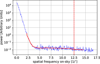
Figure 1. Summed power spectrum of the intensity, computed at a wavelength of 6302.47 Å for each step, summed across step positions with greater than the mean continuum intensity contrast of 6.2%. The dotted blue line shows the summed power spectrum windowed by a Hann filter before computing the FFT. The solid red line shows a median filter applied to the Hann-windowed power spectrum. The dashed red vertical line indicates the frequency that equates to a spatial resolution of 008.
Download figure:
Standard image High-resolution imageWe estimate the maximal spatial resolution as 008 for this scan. There is significant power at the corresponding spatial frequency even when the Hann window is applied. We also point out that the effective spatial resolution is expected to vary across the scan, perhaps significantly, as a function of the quality of the atmospheric seeing conditions and the performance of the DKIST AO correcting it. From an inspection of the smallest structures visible in Stokes I, we estimate a spatial resolution of at least 01 (about 72 km).
3. Data Analysis and Results
3.1. Inversion Strategy
We employed the Stokes Inversion based on Response Functions (SIR) code (Ruiz Cobo & del Toro Iniesta 1992) with its Python-based parallelized wrapper (Gafeira et al. 2021) to invert the full Stokes vector in the Fe i line pair for every pixel in the data set. The first inversion setup we describe here allows us to produce approximate maps of the full data set. To achieve this, we used an inversion with one magnetic and one nonmagnetic model atmosphere per pixel element, with the contribution of each given by their respective filling factors, α. We inverted every pixel 30 times with randomized initial values in the magnetic field strength, B; line-of-sight (LOS) velocity, vLOS; magnetic inclination, γ; and magnetic azimuth, ϕ. The γ is defined as the angle between the magnetic vector and the observer's LOS (or solar normal, at disk center), while ϕ is the angle of the magnetic field vector in the plane perpendicular to the observer's LOS (i.e., in the plane of the solar surface). For each pixel, we selected the solution that had the minimum χ2. Apart from temperature, T, which had four nodes, all other parameters, including B, had only one node and thus were forced to be constant in optical depth. In this case, where only one component is magnetic, we explicitly refer to the filling factor of the magnetic component, αm , and the magnetic flux density, αm B. The T in both components was always forced to be the same assuming lateral radiative equilibrium. The microturbulent velocity, vmic, was included as a free parameter independently in each component, and although the macroturbulent velocity, vmac, was also included as a free parameter, it was forced to be the same in both components, assuming that it primarily accounts for the spectral resolution of the spectrograph.
We do not explicitly include an unpolarized stray-light component to the inversions. Instead, we adopt an inversion with two model atmospheres per pixel element, allowing the filling factor of a nonmagnetic model to encapsulate the effect of an unpolarized stray-light contribution. Unlike with GREGOR, we do not have an estimate of the unpolarized stray-light fraction (Borrero et al. 2016). Nevertheless, Campbell et al. (2021b) investigated the statistical impact a varying unpolarized stray-light fraction has on the retrieval of T, B, vLOS, and ϕ values using synthetic observations and found that only the T contrast was impacted, with the other parameters invariant.
In select cases, the inversion will require additional free parameters in order to fit the Stokes profiles with asymmetries or abnormal or complex shapes (e.g., a Stokes V profile that does not only have one positive and one negative lobe of equal amplitude). Further, the number of free parameters required may increase significantly when two magnetic components are required to reproduce the observed Stokes vector. We approached these cases with a principle of minimizing the number of free parameters as much as possible. In order to reproduce a Stokes vector that is not adequately fit by the initial inversion, we enabled SIR to choose the optimum number of nodes up to a maximum of 10 in B, vLOS, and γ and three in ϕ. We then experimented by systematically reducing the number of nodes in each of these parameters until SIR was unable to fit the profiles with a minimum number of free parameters. In these pixel-specific inversions, we repeated the inversion up to 1000 times with randomized initial model atmospheres. For clarity, in later sections, we label inversions with two magnetic model atmospheres as two-component (2C) inversions. Inversions with one magnetic and one nonmagnetic model atmosphere are labeled as one-component (1C) inversions. In 2C inversions, the nonmagnetic model atmosphere is replaced by a magnetic one.
Although, in forthcoming sections, we show the atmospheric parameters at a range of optical depths, we stress that the Fe i 6300 Å doublet is only expected to be sensitive to perturbations in γ, ϕ, B, and vLOS in the range between  and 0.0 in a significant way. A detailed analysis of the diagnostic potential of these lines in the context of other photospheric Fe i lines and their response functions is provided by Cabrera Solana et al. (2005) and Quintero Noda et al. (2021).
3.2. Case Studies
An inspection of the scans revealed an abundance of circular polarization of both positive and negative polarities, as well as small patches of linear polarization. It is also clear that there are some particularly strong, large patches of circular polarization with much weaker magnetic flux patches in their immediate vicinity. In the current work, we focus on the weaker, smaller-scale magnetic structures and curate a few case studies. We used the SIR Explorer (SIRE) tool (Campbell 2023; Campbell et al. 2023) to locate and analyze these case studies in the full-scan inversions. We define a magnetic loop as two patches of opposite-polarity circular polarization in close contact (i.e., within only a few pixels of each other) with linear polarization connecting them. This definition indicates that we have two vertical fields (identified by the two opposite-polarity circular polarization signals) that are connected with a horizontal field (identified by the linear polarization signals) to complete the loop. These structures could be Ω- or U-shaped loops. In the absence of linear polarization signals, we regard the structure as a bipole. In addition to magnetic loops, we also identify unipolar magnetic flux patches with linear polarization signals but only one polarity of circular polarization. Finally, we define a serpentine structure as one with more than one PIL and clear linear polarization signals at each PIL. We further classify serpentine magnetic configurations by the number of PILs they have.
In total, we identified 53 small-scale magnetic elements of interest, including at least 47 magnetic loops and four unipolar magnetic patches, with linear and circular polarization detected in all of them. We located several candidate serpentine structures, but by examining the azimuth, we were able to discern that they were in fact two magnetic loops in close contact due to a sharp discontinuity in azimuth values. In two of the remaining serpentine-like magnetic elements, the polarity of the magnetic field appeared to change three times across the structures, and in one, it changed only twice. However, only one serpentine structure had linear polarization throughout and at all three PILs. In the following sections, we define three case studies from this analysis. We unveil the potential detection of a serpentine magnetic structure in Section 3.2.1, discuss the problem of degenerate solutions at the PILs of magnetic loops in Section 3.2.2, and analyze a magnetic granule in Section 3.2.3. Overview maps of these case studies are shown in Figure 2. The top row shows the serpentine magnetic structure, the two middle rows show two magnetic loops with transverse magnetism at the PIL, and the bottom row shows the magnetic granule. Defined here is the total linear polarization,

where λr and λb are the red (6302.7 Å) and blue (6302.3 Å) limits of integration in wavelength across the 6302.5 Å line, while Ic is the Stokes I signal measured in the neighboring continuum and spatially averaged along the slit direction for each scan step. Here we also show maps of the azimuth, which we have postprocessed to force the values to vary between 0° and 180°. We stress that we have not disambiguated the data.

Figure 2. Three case studies of small-scale magnetism, including a serpentine-like magnetic configuration (top row), two magnetic loops (middle rows), and a magnetic granule (bottom row). From left to right is Stokes I at 6303.17 Å, Ltot, Stokes V at 6302.45 Å, vLOS, γ, ϕ, and αm B. The last four parameters are derived from SIR inversions with one magnetic and one nonmagnetic model atmosphere (1C configuration). The scanning direction (i.e., solar X) is shown on the x-axis, and the slit direction (i.e., solar Y) is shown on the y-axis. The labeled (A.1, B.1, B.2, C.1–C.4) markers highlight the spatial locations of the sample pixels; the full Stokes vector from pixel A.1 is shown in Figure 3, B.1 is shown in Figure 5, B.2 is shown in Figure 6, C.1 is shown in Figure 7, C.2 is shown in Figure 8, and the circular polarization profiles for C.3 and C.4 are shown in Figure 9. The region outlined by the cyan box in the top row is shown in Figure 4.
Download figure:
Standard image High-resolution image3.2.1. Case Study I: Small-scale Serpentine Magnetism
The first case study is shown in the top row of Figure 2. Upon initial examination at a wavelength of 6302.39 Å, this appeared to be a magnetic loop, where two patches of circular polarization are in close contact, and linear polarization bridges the two patches. Upon closer inspection, a small adjustment in the wavelength position in SIRE reveals a circular polarization pattern that is more complex than a single magnetic loop. When inspected at a wavelength of 6302.45 Å, closer to the rest wavelength of the line, as shown in Figure 2, the complexity of the magnetic topology in this structure became apparent.
If one examines the γ map, it is clear that the polarity of the magnetic field changes sign at least three times across the structure (as opposed to once, as would be expected in a simple U- or Ω-shaped loop). When the pixels in this structure have reasonably symmetrical, two-lobed Stokes V profiles and linear polarization is abundant, the change in γ is unambiguous, and SIR produces good fits to the observed Stokes vectors. However, there is a narrow location at which complex Stokes V profiles are found, and the initial inversion is unable to fit these profiles. A sample Stokes vector from this location, at the edge of the granule, whose spatial location is highlighted by the marker in Figure 2, is shown in Figure 3. This Stokes vector has all three polarization parameters with signal greater than the 4σn level, but the Stokes V profile has two negative lobes. We therefore increased the number of free parameters permitted in B, γ, and vLOS to 10 each and in ϕ to three, repeated the inversion with 200 randomized initializations per pixel, and systemically reduced the number of nodes in each parameter. We found that the best fits could be achieved with one node in B but three each in γ and vLOS for the magnetic component. For the nonmagnetic component, we found that only two nodes in vLOS were required. The synthetic vector shown in Figure 3 resulted from this process. We then ran the inversion with this configuration in a small area, shown in Figure 4, so we could investigate how γ changed as a function of optical depth.
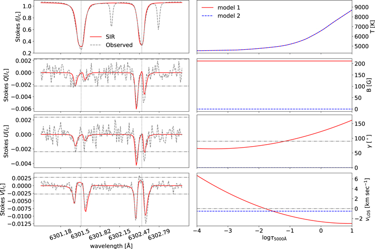
Figure 3. Sample observed Stokes vector with the best-fit inverted profiles (left panels) and model-associated atmospheres (right panels) whose spatial location is labeled in the serpentine magnetic element in the top row of Figure 2 (pixel A.1). The horizontal dotted–dashed lines show the noise thresholds (±4σn ), while the vertical dotted lines indicate the rest wavelengths of the Fe i doublet. The retrieved atmospheric parameters are shown as a function of optical depth. The ϕ, αm , and vmac values are 107°, 0.47, and 0.015 km s−1, respectively. This inversion is a 1C configuration.
Download figure:
Standard image High-resolution image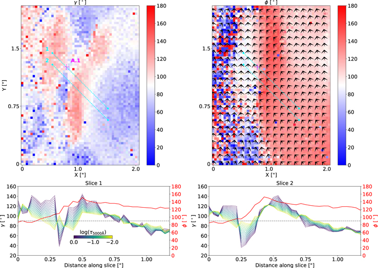
Figure 4. Maps of γ (top left) and ϕ (top right) in the serpentine structure shown in the first case study of Figure 2. The γ map is shown at  . The direction of ϕ is marked with arrows whose value is given after binning by a 3 × 3 kernel for visual clarity. The azimuth is defined such that a value of zero is aligned along the line from solar east to west, increasing counterclockwise. The variation in γ and ϕ is also shown across slices labeled 1 (bottom left) and 2 (bottom right) whose initial and final locations are indicated by the blue dashed lines. The dotted lines show the variation in γ at optical depths between
  and 0.0, while the solid red lines show the variation in ϕ across the slices. The dashed gray horizontal lines mark the 90° polarity inversion point for γ.
Download figure:
Standard image High-resolution imageShown in Figure 4 is the variation in γ across two 122 (882 km) slices generated by cubic interpolation between two points as a function of optical depth between  and 0.0, where the spectral line is expected to be responsive to changes in γ according to the response functions. Regardless of the optical depth considered, the polarity of the magnetic field changes three times across the slices. However, the spatial position at which this polarity inversion occurs can depend on the optical depth. We emphasize that this is occurring on a small, subgranular scale, as from the point where the first polarity inversion occurs to the last is a distance of about 400 km in slice 1.
To truly characterize this magnetic element as serpentine, we must also examine the azimuth. If the azimuth shows a sharp, discontinuous change between two distinct values, this could indicate that we have actually observed two separate magnetic loops that are not connected. Figure 4 also shows the variation in ϕ across the slices. In the upper (lower) slice, ϕ varies smoothly from a minimum of 86° (84°) to a maximum of 151° (153°). To confidently constrain the azimuth, one needs to measure both Stokes Q and U. However, the amplitude of the noise in the weaker linear polarization parameter places a limit on the value that ϕ could take when only one is confidently measured. Therefore, in these cases, and especially when the amplitude of the stronger linear polarization parameter is large, the ϕ value can still be constrained. When heavily noise-contaminated, maps of ϕ appear random. The map of ϕ in Figure 4 is smoothly varying across the magnetic element, including in those pixels where only one linear polarization parameter has a maximum amplitude greater than 4σn . This is in contrast to areas surrounding the magnetic element, where the map of ϕ has a salt-and-pepper pattern. The spatial coherence of this map indicates that there is enough linear polarization signal available in the magnetic element to constrain the azimuth and deduce that it varies across the slices. While a change of 69° in ϕ is not an insignificant variation, we note that the change occurs gradually. This suggests that the magnetic field vector is changing direction not just along the LOS but also in the plane of the solar surface across the slices, but not in a sharp, discontinuous way that would indicate the existence of two distinct magnetic elements. Indeed, after the ϕ value reaches its peak in each slice, it continues to vary gradually.
We also repeated the inversion in the small area in Figure 4 where the maximum number of nodes in B in the magnetic component was increased from one to three, and the maximum number of nodes in vLOS in the nonmagnetic component was increased from two to three. We found that the increased number of free parameters made a very marginal improvement in the quality of the fits in a small number of pixels but made no significant difference in the γ or ϕ variations in this magnetic element; most importantly, the polarity of the magnetic field changed three times across both slices. We found no evidence that SIR made use of the additional free parameter in vLOS.
3.2.2. Case Study II: Degenerate Solutions at PILs
One of the most likely places to find complex, abnormal Stokes profiles (i.e., a larger or smaller number of lobes than expected, with significant asymmetries, or both) in the quiet Sun is at or near the PIL in magnetic loops. In the middle rows of Figure 2, we group together two simple magnetic loops for the second case study. These structures have in common that linear polarization is found at the PIL; however, they differ significantly in terms of their circular polarization signals at the same location. The magnetic loop shown in the second row of Figure 2 is found in the intergranular lane (IGL) next to a tiny granule. From the azimuth map, we can immediately determine that this magnetic loop is a distinct structure compared to its surroundings. The sample Stokes vector B.1 shown in Figure 5 demonstrates that the linear polarization signals are strong, with small asymmetries, while the circular polarization signal has a three-lobed shape, and SIR is unable to reproduce it without an increase in the number of free parameters. The middle panels in Figure 5 show the atmospheric parameters that resulted in a good fit to the observed Stokes vector with two magnetic model atmospheres (2C), including one node in B, two in vLOS, two in γ, and one in ϕ per model. SIR has selected one magnetic component with a larger filling factor (α = 0.93) that is weaker (B = 133 G) to coexist with another magnetic component with a much smaller filling factor (α = 0.07) and much stronger magnetic field (B = 902 G). The superposition of the opposing linear stratifications in vLOS and γ is essential to produce the synthetic vector, in particular to produce the circular polarization profile that could result both from the mixing of opposite-polarity Stokes V signals within the spatiotemporal-resolution element and from gradients in vLOS. Reducing the number of nodes in either of these parameters significantly degraded the fit.

Figure 5. Two solutions to the Stokes vector belonging to pixel B.1 based on two magnetic models (2C) and one magnetic model (1C). The Stokes V signal has a complex shape. In the left column, the red solid lines show the synthetic Stokes vector for 2C, and the blue dotted lines show the same for 1C. The model parameters for 2C and 1C are shown in the middle and right columns, respectively. The location of this pixel is indicated in Figure 2. For 2C, the α values of models 1 and 2 are 0.93 and 0.07, respectively; the ϕ values are 27° and 191°, respectively; and the vmac is 0.77 km s−1 for both models. For 1C, the α values of models 1 and 2 are 0.17 and 0.83, respectively; the ϕ value is 22°; and the vmac is 0.94 km s−1 for both models.
Download figure:
Standard image High-resolution imageThis sample pixel is not unique in this magnetic loop, as many similar Stokes V profiles are found along the PIL. Furthermore, the solution provided by the inversion is not unique, and the mixing of two magnetic components in the spatiotemporal-resolution element is not the only physical scenario that could be responsible for this Stokes vector. We encounter a degeneracy problem, where very different physical solutions provide equally plausible fits to the observed Stokes vector, when trying to fit complex profiles. In Figure 5, we also present an alternative, degenerate solution that does not require a 2C configuration. In this case, a 1C configuration with a 638 G magnetic field that is constant in optical depth was sufficient, but both the magnetic and nonmagnetic model atmospheres required strong linear gradients in vLOS achieved with two nodes each, and, crucially, the magnetic model atmosphere required a polynomial stratification in γ that was achieved with five nodes.
The second magnetic loop shown in the third row of Figure 2 is a narrow patch of magnetic flux along the granule–IGL boundary. The structure is about 15 long but only 05 wide. The Stokes vector from pixel B.2 is taken from the PIL, but, in contrast to the former magnetic loop (pixel B.1), there is a complete absence of a Stokes V signal. However, despite this, we once again encounter degenerate solutions, as there are large asymmetries in the amplitudes of the σ lobes of the linear polarization profiles. Figure 6 shows solutions based on 1C and 2C configurations. These solutions have in common that SIR selected an almost perfectly transverse magnetic field. Indeed, as we have no circular polarization, we also find that there is no benefit to including a gradient in γ. In the 1C solution, we required three nodes each in B and vLOS for the magnetic model atmosphere. The αm
for this solution was very large (αm
= 0.93), and the magnetic model atmosphere is nearly stationary at the optical depths where the response functions peak, while the nonmagnetic model atmosphere has a strong downflow (vLOS = 3.8 km s−1). We find that the stratification in B, decreasing with height until reaching zero near where the response functions peak, is essential. Additionally, a linear gradient in vLOS was insufficient to fully achieve the asymmetric amplitude of Stokes Q and U. As for the 2C solution, we found it to be essential that the model atmospheres have different vLOS stratifications and ϕ values. The primary model atmosphere, with the larger filling factor (α = 0.83), has a very weak magnetic field strength (B = 28.0 G) and is nearly stationary in the LOS (vLOS = −0.1 km s−1), while the secondary model atmosphere has a polynomial stratification in vLOS and a much larger magnetic field strength (B = 676 G). We were able to reduce the number of nodes in B, γ, ϕ, and vLOS to one in both model atmospheres, with the exception of the vLOS of the secondary model atmosphere, which had three nodes and could not be reduced without losing the required asymmetries in the linear polarization profiles.
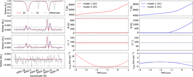
Figure 6. Same as Figure 5 but for the Stokes vector belonging to pixel B.2. For 2C, the α values of models 1 and 2 are 0.83 and 0.17, respectively; the ϕ values are 158° and 23°, respectively; and the vmac is 0.71 km s−1 for both models. For 1C, the α values of models 1 and 2 are 0.93 and 0.07, respectively; the γ and ϕ values for model 1 are 90° and 203°, respectively; and the vmac is 0.94 km s−1 for both models. There is no significant Stokes V signal.
Download figure:
Standard image High-resolution imageWe tested the inversions for pixels B.1 and B.2 under the 1C and 2C configurations, where we allowed the temperatures of both model atmospheres to vary independently. In all cases, the increase in the number of free parameters did not improve the quality of the fit; further, the key features of the parameter stratifications in B, γ, and vLOS were invariant. Ultimately, we found no evidence that increasing the number of free parameters provided either a significantly different solution or an improvement to the quality of the fit to the observed Stokes vector, so we favor the simpler solutions.
3.2.3. Case Study III: Magnetic Anatomy of a Granule
The bottom row of Figure 2 shows our final case study. Notably, we find that there is significant linear and circular polarization signal throughout almost the entirety of the granule. We take this opportunity to explore the different spectropolarimetric and magnetic properties of the granule and surrounding IGL, which is the convective building block of the solar surface, for the first time at 70 km resolution. To this end, we select four representative pixels. To begin, in the lower leftmost patch of circular polarization, the linear polarization is pervasive, while both the linear and circular polarization profiles are highly asymmetric, and the circular polarization is even single-lobed. Figure 7 shows a sample Stokes vector (pixel C.1) from this patch, with its location at the granule–IGL boundary indicated by the blue marker in Figure 2. The initial 1C inversion was unable to accurately fit the asymmetric Stokes profiles, so the number of free parameters was increased. The very good fit shown in Figure 7 is the result; it was achieved with three nodes in B, three in vLOS, three in γ, and one in ϕ for the magnetic model atmosphere and only one node in vLOS for the nonmagnetic model atmosphere. We found that a 1C configuration was sufficient and did not require a 2C configuration. The B stratification required to fit this profile is a gradient that decreases with increased height in the atmosphere, from a very strong, kG magnetic field strength (B > 2000 G) in the deepest layers. However, we stress that SIR is simply extrapolating to  . At
. At  , the field strength is 851 G. The magnetic model atmosphere (αm
= 0.79) is highly transverse in the optical depth range the lines are responsive to but has a gradient that changes polarity and becomes more vertical higher in the atmosphere. In order to produce the asymmetries in all four Stokes parameters, the magnetic model atmosphere also required a strong linear gradient in vLOS, while the nonmagnetic component has a single, positive vLOS value throughout the atmosphere.
, the field strength is 851 G. The magnetic model atmosphere (αm
= 0.79) is highly transverse in the optical depth range the lines are responsive to but has a gradient that changes polarity and becomes more vertical higher in the atmosphere. In order to produce the asymmetries in all four Stokes parameters, the magnetic model atmosphere also required a strong linear gradient in vLOS, while the nonmagnetic component has a single, positive vLOS value throughout the atmosphere.

Figure 7. Same as Figure 3 but for vector C.1. The filling factors of models 1 and 2 are 0.79 and 0.21, respectively, while the ϕ value is 146°. The vmac is 0.73 km s−1 for both models. This inversion is a 1C configuration. The Stokes V signal has a single lobe.
Download figure:
Standard image High-resolution imageDeep in the granule, in the central patch of circular polarization, the linear polarization is again pervasive, but the circular polarization is much more symmetric and two-lobed. Figure 8 shows a sample Stokes vector (pixel C.2) whose location is indicated by the cyan marker in Figure 2. The synthetic vector provided by the initial 1C inversion is a good fit in this case, with the exception of small asymmetries in the linear polarization profiles. By adding a gradient to the vLOS of the magnetic model atmosphere, SIR was able to obtain better fits. The B of this pixel is moderate, but the pixel has a large αm such that the αm B is relatively large (B = 380 G, αm = 0.31, αm B = 118 Mx cm−2). In the lower right patch of circular polarization, most of the profiles do not have significant linear polarization, and the circular polarization profiles are typically asymmetric. While the profiles may be asymmetric or not, the change in polarity is nevertheless unambiguous between these three patches of small-scale magnetism. It is perhaps not surprising that the profiles are asymmetric, and therefore indicative of velocity gradients, in pixel C.1 given that it is located at the granule–IGL boundary. Pixel C.2, on the other hand, is more firmly located in the granule.
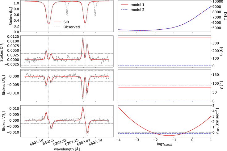
Figure 8. Same as Figure 3 but for vector C.2. The filling factors of models 1 and 2 are 0.31 and 0.69, respectively, while the γ and ϕ values are 78° and 152°. The vmac is 0.95 km s−1 for both models. This inversion is a 1C configuration. The Stokes V signal exhibits a regular double-lobed, antisymmetric shape.
Download figure:
Standard image High-resolution imageThe Stokes vectors found in the IGLs surrounding the examined granule were also inspected. Stokes V profiles with varying degrees of asymmetries are found. We find that the field strengths at these locations differ by 2 orders of magnitude, and at the high end of these extremes, B exceeds 2 kG. We are motivated to sanity-check these values with the weak and strong field approximations (WFA and SFA) in order to ensure that the inversions are well calibrated (Campbell et al. 2021a, 2023) by estimating the longitudinal magnetic flux density with the WFA and magnetic field strength with the SFA.
In the weak regime, as Landi Degl'Innocenti & Landolfi (2004) demonstrated, the amplitude of Stokes V is proportional to the longitudinal magnetic flux density (where  ),
),

where

where λ0 is the rest wavelength, and geff is the effective Landé g-factor of the spectral line. Equation (2) is only valid if the magnetic Zeeman splitting is negligible relative to the Doppler width of a line (i.e., ΔλB /Δλd ≪ 1) and when γ, ϕ, B, vLOS, the Doppler width, and any broadening mechanisms are invariant along the LOS in the formation region of the line. On the other hand, by measuring 2ΔλB as the separation of the lobes of Stokes V when the field is strong enough and ΔλB /Δλd ≫ 1, it is possible to obtain B directly through Equation (3) (Khomenko et al. 2003; Nelson et al. 2021; Campbell et al. 2023). As in Asensio Ramos (2011), writing the expressions for ΔλB and Δλd allows us to say that a line is in the weak field regime when the magnetic field strength fulfills

where m is the mass of an electron, c is the speed of light, λ0 is the rest wavelength of the spectral line, e is the charge of an electron, k is the Boltzmann constant, and M is the mass of the species. For the 6302.5 Å line, assuming vmic = 1 km s−1 and T = 5800 K, we estimate a limit of 760 G. Raising T to 7000 K would increase the limit to 809 G. Eliminating vmic would decrease the limit to 610 G.
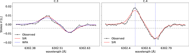
We sampled pixels at the uppermost granular boundary with low-amplitude, symmetrical Stokes V profiles and applied the WFA. The circular polarization profile from the pixel labeled C.3 in Figure 2 is shown in Figure 9. In the initial 1C inversion, SIR fit this profile with a model atmosphere with B = 73.4 G, γ = 57 0, αm
= 0.5, and vLOS = 0.1 km s−1. Therefore, according to SIR,
0, αm
= 0.5, and vLOS = 0.1 km s−1. Therefore, according to SIR,  Mx cm−2. The B value is an order of magnitude smaller than the limit we estimated using Equation (4), so we are satisfied that using the WFA on this pixel is appropriate. Meanwhile, the WFA estimate is obtained from the derivative of Stokes I and through Equation (2) as 20.0 Mx cm−2. The pixel with the weakest B that we found that satisfied the 4σn
amplitude threshold and had symmetrical lobes was 25 G, or
Mx cm−2. The B value is an order of magnitude smaller than the limit we estimated using Equation (4), so we are satisfied that using the WFA on this pixel is appropriate. Meanwhile, the WFA estimate is obtained from the derivative of Stokes I and through Equation (2) as 20.0 Mx cm−2. The pixel with the weakest B that we found that satisfied the 4σn
amplitude threshold and had symmetrical lobes was 25 G, or  Mx cm−2. For the same pixel, the WFA estimate was 11.7 Mx cm−2.
Figure 9. The Stokes V profiles from pixels C.3 and C.4 are shown in the left and right panels, respectively. Profile C.3 has the WFA fit obtained from the derivative of Stokes I (blue dashed line) overplotted. Both profiles have the synthetic SIR profile overplotted (red solid line). The horizontal gray dashed–dotted lines show the 4σn threshold, and the vertical blue dotted lines show the locations of the blue and red lobes used for the SFA estimate for B.
Download figure:
Standard image High-resolution image
We sampled pixels in the rightmost IGL, which has an extremely strong magnetic field, and applied the SFA by measuring the separation of the lobes of Stokes V. The circular polarization profile from the pixel labeled C.4 in Figure 2 is shown in Figure 9. In this case, the initial 1C inversion fit this profile with a very strong magnetic field (B = 2048 G, αm = 0.07, αm B = 139.3 Mx cm−2), and the positive and negative lobes of Stokes V are separated by 15 increments in wavelength. The SFA estimate is thus 2078 G, as a single increment in wavelength is equivalent to 138.55 G. We are satisfied both that using the SFA is appropriate and that the magnetic field strength is accurate, as there are many pixels in this IGL with field strengths greater than 1.8 kG.
4. Discussion
We have presented the first spectropolarimetric observations of the quiet Sun with DKIST, the first 4 m class and largest solar optical telescope ever built. With an estimated spatial resolution of 008, these observations represent the highest spatial resolution full-vector spectropolarimetric observations ever obtained of the quiet Sun; previous high-resolution observations were achieved by the Swedish Solar Telescope (016; e.g., Schnerr & Spruit 2011), the Sunrise balloon-borne experiment (014–016; e.g., Lagg et al. 2010; Wiegelmann et al. 2013), the GREGOR telescope (03–04; e.g., Lagg et al. 2016; Campbell et al. 2023), and the Hinode spacecraft (032; e.g., Lites et al. 2008; Bellot Rubio & Orozco Suárez 2012). After locating at least 53 magnetic elements of interest, we curated three case studies and examined their physical properties in detail to showcase how the small-scale magnetic fields are spatially organized at this resolution.
We examined a particular magnetic element where the polarity inverts three times across the structure (see Figure 4). In addition to a complex topology in terms of the inclination angle, we also observe the azimuthal angle changing significantly across its structure. We believe that the evidence indicates that it is plausible that the magnetic field lines of this small-scale magnetic structure are serpentine with significant, coherent variation in the plane of the solar surface. We are not aware of any previous studies that have observed these complex magnetic structures in the quiet Sun on a subgranular scale. Hinode observations have demonstrated that in simple magnetic loops, the azimuth can vary significantly in a few minutes (Martínez González et al. 2010), and simulations of the twisting of magnetic field lines during small-scale reconnection events show that gradual azimuthal changes in the photosphere are plausible in more complex magnetic topologies (Danilović 2009; Hansteen et al. 2017). Perhaps it is possible that these complex topologies have not been observed at facilities with lower diffraction-limited resolutions than DKIST precisely because they lack the required angular and spectral resolution. Similarly, the complex nature of the serpentine feature could be lost with poorer seeing conditions. However, we also emphasize that this is the only example of serpentine magnetism that we discovered in the data set that had three PILs and linear polarization signals throughout the structure, and in the other magnetic loops, we see a much simpler variation in γ and typically insignificant variation in ϕ.
An alternative interpretation would be that we observed two magnetic loops in very close proximity. The fact that the azimuth increases to reach a maximum in one part of the slice but then decreases somewhat less significantly in the remainder of the slice could support this argument. However, the evidence does not conclusively support this interpretation either because there is no discontinuity in the variation of the azimuth like what can be observed in the magnetic loop shown in the second row of Figure 2. We note that without disambiguation of the azimuth, we cannot be certain that the gradual, coherent variation we measure is correct. If this alternative explanation was true, we argue that we should not observe linear polarization signals at the middle apparent PIL between the magnetic loops. In other words, we should not observe linear polarization signals at all three apparent PILs. We note that linear polarization signals are pervasive across the entire slice; thus, we are able to observe two crests in the magnetic field lines. However, we also note that we discovered a second serpentine structure with three PILs in our analysis, and the middle PILs did not have linear polarization signals.
Ultimately, only repeated observations with a high-cadence time series would allow us to conclusively determine the correct scenario. Finally, we point out that the temporal resolution may play a role due to the scanning speed of the observations. The step cadence of these scans is about 7.4 s. A horizontal flow would have to be on the order of 4 km s−1 to be similar to the stepping cadence. However, it would be premature to say that this is a factor that makes either scenario less or more plausible; for instance, the gradual variation in the azimuth that we measured could be explained by supposing that we observed the temporal evolution of a serpentine structure.
A physical scenario that demands an increased number of free parameters commonly occurs at the PIL of magnetic elements, and detecting linear polarization at these locations has been a major challenge (Kubo et al. 2010, 2014). We examined two magnetic loops that had very different properties at the PIL in terms of circular polarization but both had strong linear polarization signals. In one case, we uncovered a Stokes vector that had a complex Stokes V profile. Three-lobed Stokes V profiles were also observed in the quiet Sun by Viticchié & Sánchez Almeida (2011) with Hinode/SP and Martínez González et al. (2016), Kiess et al. (2018), and Campbell et al. (2021a) with GREGOR. Initially, we attempted a 2C inversion, but with gradients in γ, as well as in B and vLOS (see Figure 5). We encountered a problem of degeneracy, as we found that this profile could also be explained with a more extreme gradient in γ but without two magnetic model atmospheres (see Figure 5). The second interpretation is consistent with Khomenko et al. (2005), who showed using magnetoconvection simulations that gradients in γ and vLOS can generate irregular Stokes V profiles. In this case, it is not as simple as saying the approach with the lower number of free parameters is the correct one; the fact that this profile was located along the PIL means it is plausible that the three-lobed Stokes V profile is the physical manifestation of a smearing of signals of opposite polarities or even mixing within the spatiotemporal-resolution element of the observations that remains unresolved. We note that in the 1C case, γ changes polarity along the LOS in the optical depth range in which these lines are sensitive to perturbations in γ, and there are other examples in this study where this occurs (see Figures 3 and 7). Previously, Rezaei et al. (2007) showed that this was possible when the Fe i 6301.5/6302.5 Å doublet showed two-lobed Stokes V profiles with different polarities in a single spectrum, but in our observations, we find that the Stokes V profiles of both lines are compatible.
In another case, we observe a long, narrow magnetic loop at the granule–IGL boundary that has an absence of Stokes V at the PIL. It is most plausible that in this case, the magnetic field at the PIL is completely transverse; however, like in the former example, opposite-polarity Stokes V signals may have mixed such that their signals have completely canceled each other out. However, the absence of a Stokes V signal cannot be presented as evidence for the latter scenario. We also find degenerate solutions to this Stokes vector based on a single magnetic model and two magnetic models (see Figure 6), showing that degeneracy is an issue even in the absence of a Stokes V profile. This degeneracy issue is a serious problem that calls into question how accurately we can infer physical parameters from inversions, but we argue that this issue could be significantly improved by observing more photospheric spectral lines. This is distinct from the degeneracy problem described by Martínez González et al. (2006) because in all of the inversions presented in this study, we forced the temperature of each component to be the same. Ultimately, if the solutions requiring two magnetic models are correct, it suggests that, even at the spatiotemporal resolution of DKIST/ViSP, magnetic flux is yet hidden to spectropolarimetric observations that use the Zeeman effect in magnetic loops (or bipoles).
Significant effort was made to try and balance the need for an increased number of free parameters to fit complex Stokes profiles with the risk of producing unphysical or unrealistic solutions from the inversions. In particular, velocity gradients in the LOS often manifest in Stokes Q, U, and V as an amplitude asymmetry that cannot be modeled with a vLOS stratification that is constant in optical depth. In the final case study, we examined a magnetic feature spanning a granule that had linear polarization signals throughout most of its structure. The magnetic nature of granules is important because it has implications for constraining magnetohydrodynamic simulations, particularly in terms of circulation models, emergence of magnetic flux, and the formation of IGLs (Rempel 2018). It is notable that this granule has pervasive linear polarization, in addition to circular polarization, because magnetic flux emergence in granules was observed in early Hinode/SP observations to be longitudinal in nature (Orozco Suárez et al. 2008), but the emergence of horizontal magnetic flux has been observed in a granule (Gömöry et al. 2010). In the granule, we found symmetric Stokes profiles (see Figure 8), but at the granule–IGL boundary, we sampled a Stokes vector from a pixel that had significant asymmetries in the polarization parameters (see Figure 7). We inverted this Stokes vector with an approach that sought to minimize the number of free parameters as much as possible but were only adequately able to reproduce it using gradients in B, γ, and vLOS. Single-lobed Stokes V profiles are common in quiet Sun Hinode observations, accounting for up to 34% of the profiles (Viticchié & Sánchez Almeida 2011). They cover about 2% of the surface, are associated with inclined magnetic fields and flux emergence and submergence processes, and are reproduced by simulations (Sainz Dalda et al. 2012). There is an expectation that the existence of canopy fields means that the magnetic field becomes statistically more horizontal with height (Stenflo 2013; Danilovic et al. 2016). However, in our analysis, we found the opposite in individual cases (see Figures 3 and 7). Although it is well understood that depth-averaged parameters can be well retrieved from inversions of photospheric diagnostics without the inclusion of gradients in the magnetic or kinetic parameters (see, for instance, Campbell et al. 2021b; Quintero Noda et al. 2023), we offer a word of caution that at DKIST resolutions, it is clear that any future statistical analysis of these data will be inadequate unless the need for gradients in vLOS (and other parameters) is accounted for in the inversions due to their prevalence in these small-scale magnetic structures.
We sampled relatively symmetric circular polarization profiles at the granular boundaries of the magnetic granule—with one side of the granule harboring smaller-amplitude profiles, indicative of a weak magnetic field, and the other with amplitudes twice their size and much larger lobe separations—and applied the WFA and SFA to retrieve manual estimates of αm B and B. This allowed us to sanity-check our measurements of vastly different magnetic field strengths spanning 2 orders of magnitude. However, we note that the difference in αm B is not as large as the difference in B, indicating that the determination of αm plays a role. However, we expect that inversions of these lines are able to constrain both αm and B (Asensio Ramos 2009) and expect to be able to make distinctions between weak and strong fields in these lines when αm is a free parameter (del Toro Iniesta et al. 2010). We emphasize that such symmetrical Stokes V profiles are in the minority in this structure, especially in the IGLs, so we do not recommend attempting to apply these approximations more broadly to these data except in limited specific cases. The extremely large field strengths we recorded are at the high end of what is expected to result from magnetic field amplification in bright points based on high-resolution spectropolarimetric observations (see, for instance, Beck et al. 2007; Utz et al. 2013; Keys et al. 2019).
The analysis presented in this study was conducted under the assumption of local thermodynamic equilibrium (LTE). Smitha et al. (2020) showed that for the Fe i 6300 Å doublet, there can be departures from LTE due to resonance line scattering and overionization of Fe atoms by ultraviolet photons. The former process makes the line stronger, while the latter makes the line weaker, which means that for the Fe i 6300 Å doublet, these processes compensate for each other to an extent. Nevertheless, departures from LTE can introduce errors or uncertainties in the derived atmospheric parameters.
5. Conclusions
We have analyzed spectropolarimetric observations of the quiet Sun with the first 4 m class optical telescope in service to solar physics. This allowed us to reveal, for the first time, the serpentine nature of the subgranular, small-scale magnetic field, as we demonstrated that the polarity of the magnetic field changed at least three times in only 400 km. The three polarity reversals are evident from an inspection of the Stokes V profiles and confirmed by the inversions. From the inversions, we were also able to deduce that the azimuth changed in a significant but coherent way. While beyond the scope of this study, it is clear that a statistical analysis based on a non-LTE inversion, not just of the Ca ii 8542 Å line but also the Fe i doublet, is the next logical step and will be the subject of future work. We were unable to trace the temporal evolution of these structures. Observations of these structures at high cadence (30–90 s) should be a priority for DKIST in the future with the Diffraction Limited Near Infrared Spectropolarimeter instrument (Jaeggli et al. 2022).
We found that, particularly at the PILs of magnetic loops, degenerate solutions in inversions remain a significant issue even at the spatial resolution provided by a 4 m telescope, and this is true even in the absence of a Stokes V signal. Although previous work involving simulations and synthetic observations has shown that atmospheric parameters can be well recovered, on average (see, for instance, Campbell et al. 2021b; Quintero Noda et al. 2023), in our case studies, we found that to truly characterize the plasma on small scales, we had to permit a larger number of free parameters to produce the required asymmetries in the Stokes profiles and abnormal Stokes V profiles. We are unable to distinguish between gradients in atmospheric parameters along the LOS and smearing of signals in the plane of the solar surface due to the spatial point-spread function of the telescope. We concur with the advice provided by Cabrera Solana et al. (2005) and Quintero Noda et al. (2021) and suggest that observations of the Fe i 6302.5 Å line with the deep photospheric Fe i 15648.5 Å line should be prioritized, as observations of diagnostics that sample a range of heights in the photosphere could provide a method for distinguishing between these two otherwise plausible scenarios when simultaneously inverted. These observations would additionally benefit from the demonstrated ability of the Fe i 15648.5 Å line to observe higher linear polarization fractions (Martínez González et al. 2008b; Lagg et al. 2016; Campbell et al. 2023).
Acknowledgments
We thank the anonymous referee for the suggestions that improved this manuscript. R.J.C., D.B.J., and M.M. acknowledge support from the Science and Technology Facilities Council (STFC) under grant Nos. ST/P000304/1, ST/T001437/1, ST/T00021X/1, and ST/X000923/1. D.B.J. acknowledges support from the UK Space Agency for a National Space Technology Programme (NSTP) Technology for Space Science award (SSc 009). D.B.J. and M.M. acknowledge support from Leverhulme Trust grant RPG-2019-371. This research has received financial support from the European Union's Horizon 2020 research and innovation program under grant agreement No. 824135 (SOLARNET). R.E. is grateful to STFC under grant No. ST/M000826/1 and acknowledges NKFIH (OTKA, grant No. K142987) Hungary for enabling his contribution to this research. The research reported herein is based in part on data collected with the Daniel K. Inouye Solar Telescope (DKIST), a facility of the National Solar Observatory (NSO). The NSO is managed by the Association of Universities for Research in Astronomy, Inc., and funded by the National Science Foundation. Any opinions, findings, and conclusions or recommendations expressed in this publication are those of the authors and do not necessarily reflect the views of the National Science Foundation or the Association of Universities for Research in Astronomy, Inc. DKIST is located on land of spiritual and cultural significance to Native Hawaiian people. The use of this important site to further scientific knowledge is done with appreciation and respect. This material is based upon work supported by the National Center for Atmospheric Research, which is a major facility sponsored by the National Science Foundation under cooperative agreement No. 1852977.
The observational data used during this research are openly available from the DKIST Data Centre Archive 10 under proposal identifier pid_1_36.
Facility: DKIST - (Rimmele et al. 2020).
Software: SIR explorer 11 (Campbell 2023), Astropy (Astropy Collaboration et al. 2022), Matplotlib (Hunter 2007), Numpy (Harris et al. 2020).
Footnotes
- 9
Version 2.0.2 of the ViSP level 0 to level 1 pipeline was used.
- 10
- 11