


Abstract
We use observations from the Magnetospheric Multiscale spacecraft to identify a free energy source for high-frequency whistler waves in the Earth's quasi-perpendicular bow shock. In the considered measurements, whistlers propagate both parallel and antiparallel to the background magnetic field B0 with frequencies around 100 Hz (0.15 fce, where fce is the electron cyclotron frequency) and amplitudes between 0.1 and 1 nT. Their growth can be attributed to localized pitch angle anisotropy in the electron velocity distribution function that cannot be precisely described by macroscopic parameters like heat flux or temperature anisotropy. However, the presence of heat flux along −B0 does create preferential conditions for the high-frequency whistler waves that propagate in this direction. These waves are directed partially toward the shock, meaning they can scatter electrons that are streaming from the shock. This prolongs the time the electrons spend in the shock transition region and thereby promotes electron energization.
Export citation and abstract BibTeX RIS
1. Introduction
Remote observations have shown that supernova remnant shocks can accelerate electrons to highly relativistic energies (Koyama et al. 1995; Bamba et al. 2003). In principle, the particles are energized by diffusive shock acceleration—they cross and gain energy from the same shock multiple times due to small-angle scattering from Alfvén waves on either side (e.g., Blandford & Eichler 1987). For this process to be viable for electrons, they must have gyroradii that are larger than the typical ion gyroradius (e.g., Ellison & Reynolds 1991), which implies they must have energies that are orders of magnitude above thermal.
Several mechanisms have been proposed for accelerating electrons to highly suprathermal energies in collisionless shocks. Electrons can be energized in the shock transition region by electrostatic waves produced, for example, by the Buneman instability (Cargill & Papadopoulos 1988; Amano & Hoshino 2009). However, it is not clear whether this process can operate at realistic background plasma parameters (Riquelme & Spitkovsky 2011), which critically affect the development of electrostatic instabilities (e.g., Wang et al. 2020; Wilson et al. 2021; Vasko et al. 2020). Alternatively, oblique low-frequency whistler/magnetosonic waves can accelerate electrons in the shock foot (Riquelme & Spitkovsky 2011).
A common feature of the proposed energization processes is electron confinement to the shock transition region, which prolongs the time available for mechanisms like shock drift acceleration to act. For example, hybrid simulations of high Mach number shocks show that electron scattering (Burgess 2006) or guiding (Guo & Giacalone 2010) by ion-scale magnetic field fluctuations in the transition region can lead to greater energy gain than in the absence of fluctuations. Katou & Amano (2019) pointed out that pitch angle scattering from whistler waves propagating along the background magnetic field may also confine electrons, and established the frequency-dependent minimum wave power needed for this scenario to be viable.
The Earth's quasi-perpendicular bow shock accelerates electrons to energies that are orders of magnitude higher than thermal (e.g., Anderson et al. 1979; Gosling et al. 1989; Oka et al. 2006), so serves as a natural laboratory for studying the energization mechanisms that have been identified in simulations and theoretical work. Recently, Amano et al. (2020) showed that the whistler power required for electron confinement by pitch angle scattering can be exceeded here for frequencies at least up to 0.1 fce (fce is the electron cyclotron frequency). Higher frequency whistlers are necessary for scattering electrons in lower energy (≲1 keV), higher density regions of velocity space. These electrons subsequently gain energy, after which they can interact with lower frequency whistlers or ion-scale fluctuations and proceed further up the energy ladder. The efficiency of electron energization in collisionless shocks therefore may be sensitive to the level of high-frequency whistler power, which stimulates analysis of the origin and properties of these waves.
Pioneering in situ spectral measurements in the Earth's bow shock revealed magnetic field fluctuations in the whistler frequency range (e.g., Rodriguez & Gurnett 1975). Later observations showed that whistlers with frequencies on the order of 0.1 fce typically propagate quasi-parallel to the background magnetic field B 0 and are present in the upstream, shock transition, and downstream regions. Their amplitudes are generally less than 0.01 ∣B0∣ (Zhang et al. 1999; Hull et al. 2012; Oka et al. 2017), but occasionally are as large as 0.1 ∣B0∣ (Zhang et al. 1999; Wilson et al. 2014).
Although these studies established the presence and basic properties of high-frequency whistler waves in the Earth's bow shock, there has been scarce research into their origin. Some studies have advanced temperature anisotropy or electron beams as their free energy source (Tokar et al. 1984; Hull et al. 2012), but a lack of high-cadence electron data has prevented experimental tests of these proposals.
In this Letter we examine whistler waves measured by the Magnetospheric Multiscale (MMS) spacecraft in the Earth's quasi-perpendicular bow shock. We find that the waves are generated locally due to electron pitch angle anisotropy. Importantly, the observations demonstrate that the presence of electron heat flux is associated with intense high-frequency whistler waves. Pitch angle scattering from these waves can cause the energization of electrons in low energy, dense regions of velocity space that are not as accessible to ion-scale scattering agents.
2. Data and Methods
The MMS constellation consists of four spin-stabilized spacecraft on elliptical orbits through the Earth's magnetosphere (Burch et al. 2016). We only present measurements from MMS1 because the other MMS spacecraft, being within a few tens of kilometers of MMS1, observed similar dynamics. We use magnetic field waveforms captured at 8192 S s−1 (samples per second) by a tri-axial search-coil magnetometer (Le Contel et al. 2016), electric field waveforms measured at the same cadence by double probes in the spin plane (Lindqvist et al. 2016) and along the spin axis (Ergun et al. 2016), and 128 S s−1 DC magnetic field measurements from a fluxgate magnetometer suite (Russell et al. 2016).
The electron and ion velocity distribution functions (VDFs) are measured every 30 and 150 ms, respectively, by the Fast Plasma Investigation (FPI) instrument (Pollock et al. 2016). We use electron pitch angle distributions (PADs) that are constructed from the full 3D electron VDFs with 18 pitch angle bins and 32 energy bins. The instrument's nominal electron energy range extends from 5 eV to 30 keV, but we discard high energy measurements that are below the one-count level and low energy measurements that are contaminated by photo and secondary electrons, leaving a band that extends from about 10 eV to 1 keV. The energy bin centers are log-spaced with a ratio of about 1.3, giving 18 bins in this range. We also use density, temperature, and heat flux moments of the distribution functions provided by the FPI team.
The electron VDFs in the Earth's bow shock cannot generally be modeled as the sum of Maxwellian and Kappa distributions (e.g., Montgomery et al. 1970), so standard dispersion relation solvers cannot be used to examine the plasma stability. We instead use Linear Electromagnetic Oscillations in Plasmas with Arbitrary Rotationally-symmetric Distributions (LEOPARD), a generalized solver for gyrotropic distributions (Astfalk & Jenko 2017).
As input, LEOPARD requires a distribution function f(v∥, v⊥) sampled on a grid that is linearly spaced in velocity perpendicular (v⊥) and parallel (v∥) to
B
0. To convert the measured PADs to this format, we perform an interpolation of  that is quadratic in energy and pitch angle using the "RectBivariateSpline" function from the Python package SciPy (Virtanen et al. 2020). Figure 1 demonstrates that the interpolation gives a plausible representation of the VDF. Density and temperature moments calculated using the interpolation are within 5% of the moments provided by the FPI team.

Figure 1. From an electron VDF measured downstream of the shock, the interpolated and empirical phase space density as a function of energy at several pitch angles. Pitch angle anisotropy is present within the black rectangle in the top panel, which is magnified in the bottom panel. The solid lines are cuts through a bivariate quadratic spline interpolation of the phase space density data, which are marked with dots. At pitch angles coinciding with the data point pitch angles (15°, 25°, and 35°), the spline passes through the data points and captures their energy dependence in a parsimonious manner. At intervening pitch angles (20° and 30°), the interpolation lines appropriately lie between the lines at 15°, 25°, and 35°.
Download figure:
Standard image High-resolution image3. Results
On 2017 November 2 around 08:29:00 UT, MMS1 crossed the bow shock near the ecliptic plane at the flank, as depicted in Figure 2. Measurements from this shock crossing have been previously considered in the context of electrostatic fluctuations (Vasko et al. 2020; Wang et al. 2021). Analysis of the Rankine–Hugoniot jump conditions using the Viñas & Scudder (1986) algorithm showed that it is a quasi-perpendicular supercritical shock with θBn ≈ 110°, Alfvén Mach number MA ≈ 5, and upstream electron beta βe ≈ 1.6.

Figure 2. Schematic of the Earth's bow shock in the ecliptic plane with the data collection site indicated. This site is also displaced out of the ecliptic plane by 6 Re (Earth radii). The shock normal n was determined using the Viñas & Scudder (1986) algorithm. In Geocentric Solar Ecliptic (GSE) coordinates, n = (0.76, 0.63, 0.17).
Download figure:
Standard image High-resolution imageFigure 3 presents an overview of the measurements taken by MMS1 in the shock ramp and downstream regions. Panel (a) shows the three components of the background magnetic field in Geocentric Solar Ecliptic (GSE) coordinates, as well as the field magnitude. We note that in the upstream and downstream regions, the component of the magnetic field along the shock normal is directed toward downstream. The field magnitude increases by a factor of 2–3 across the shock ramp, as do the electron density and temperature, which are shown in panels (b) and (c). Panel (b) also shows the magnitude of the magnetic field-aligned electron heat flux, normalized by a constant free-streaming value,  , where downstream density and temperature values of 50 cm−3 and 40 eV were used to compute q0. The electron heat flux is antiparallel to the magnetic field, so it is directed toward the shock, and its magnitude remains between about 0.1 and 0.2 q0 throughout the downstream region. Panel (c) presents the electron temperature anisotropy and demonstrates that electrons are macroscopically more or less isotropic after 08:29:30 UT with 0.9 ≲ T⊥/T∥ ≲ 1.1.

Figure 3. Overview of MMS1's measurements in the bow shock. (a) The magnitude and three vector components of the background magnetic field in Geocentric Solar Ecliptic coordinates. (b) In blue, the electron density moment and, in black, the heat flux projected along B 0 and normalized by q0 = 0.6 mW m−2, the average downstream free-streaming value. (c) In blue, the electron temperature moment and, in black, the macroscopic temperature anisotropy. (d) The power spectral density of the 8192 S s−1 magnetic field measurements. The two green lines mark 0.1 fce and 0.2 fce. (e) All of the observed wave power has an ellipticity approximately equal to +1, meaning it is right-handed and circularly polarized. (f) The wave normal angle with respect to B 0. All of the observed waves propagate approximately parallel (θkB = 0°) or antiparallel (θkB = 180°) to B 0. The black wedges below each panel mark the times of the waves presented in Figure 4.
Download figure:
Standard image High-resolution imagePanels (d)–(f) present a spectral analysis of the 8192 S s−1 electric and magnetic field waveforms. The basis of the analysis is a short-time Fourier transform using a Hann window with a 0.1 s width. Panel (d) shows the average power spectral density (PSD) of the three magnetic field components and demonstrates the presence of intense wave activity between 0.1 and 0.2 fce. Panel (e) shows the ellipticity computed using singular value decomposition (SVD) of the magnetic field spectral matrices (e.g., Santolík et al. 2003). The observed wave power has an ellipticity close to +1, which indicates circular polarization and right-handed rotation with respect to B 0, confirming that these are whistler waves. Panel (f) shows the wave normal angle θkB with respect to B 0. SVD is used to determine the propagation axis ± k of the wave power, and cross-spectral analysis of the spin plane magnetic and electric fields is used to pick out the correct propagation direction k along this axis. Before 08:30:00, the waves are seen to propagate mostly antiparallel to B 0, θkB ≈ 180°, meaning they are aligned with the electron heat flux and typically travel toward the shock. At later times, further from the shock, waves propagating parallel to B 0 are observed as well.
Figure 4 presents an analysis of the origin of a few particular whistler waves. Panels (a) and (b) show the electric (Ex ) and magnetic (Bx ) field fluctuations of an antiparallel whistler wave observed around 08:29:52 UT and a parallel whistler wave observed around 08:30:21 UT. In accordance with the waves' propagation directions, Ex leads Bx by 90° in panel (a), and lags Bx by 90° in panel (b). Panels (c) and (d) present electron VDFs f(v∥, v⊥) associated with the whistler waves. Pitch angle anisotropy is present in regions where the contours of constant f(v∥, v⊥) do not follow contours of constant energy. These regions can potentially contribute to whistler wave growth (e.g., Kennel 1966; Kennel & Petschek 1966).
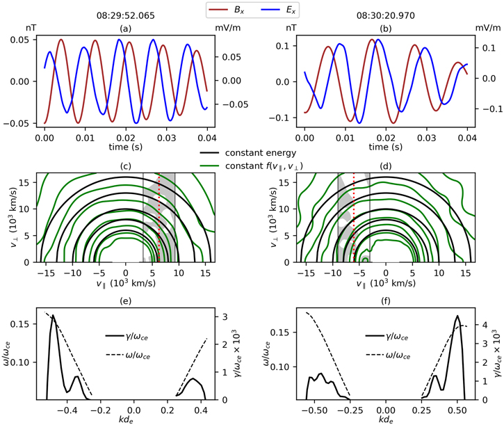
Figure 4. Simultaneous field and particle measurements for a wave propagating antiparallel (left column) and parallel (right column) to B 0. Panels (a) and (b): electric and magnetic field fluctuations bandpass filtered between 100 and 140 Hz in panel (a) and between 80 and 120 Hz in panel (b). Panels (c) and (d): coinciding electron VDFs. These panels are masked at energies <10 eV, where there is no accurate electron data available. Contours of constant phase space density f(v∥, v⊥) are shown in green and contours of constant energy in black. Panels (e) and (f): results of the stability analysis on the VDFs in panels (c) and (d), respectively. These panels show the growth rate γ/ωce versus kde (solid lines) and dispersion relation ω/ωce vs kde (dashed lines) for antiparallel (k < 0) and parallel (k > 0) whistler waves, where de = c/ωpe is the electron inertial length, ωce is the angular electron cyclotron frequency, and ωpe is the angular electron plasma frequency. The red vertical lines in panels (c) and (d) mark the resonant velocities of the fastest growing modes. The gray shading marks the regions of the VDFs near resonance that have the appropriate velocity space gradient for particles to give energy to the fastest growing wave (see Section 3 for details).
Download figure:
Standard image High-resolution imagePanels (e) and (f) present the results of the stability analysis. At both moments, 08:29:52 and 08:30:21 UT, parallel and antiparallel whistler waves are both unstable, but one propagation direction has a higher maximum growth rate by a factor of 3–4. At 08:29:52 UT, antiparallel whistler waves at frequencies f ≈ 0.15fce have the largest growth rate, γ ≈ 3 · 10−3 ωce, which is consistent with the presence of an antiparallel wave in the coinciding field measurements. At 08:30:21 UT, the fastest growing mode has γ ≈ 4 · 10−3 ωce and propagates parallel to B 0, which is again in agreement with field measurements.
The instabilities driving the whistler waves are neither heat flux nor temperature anisotropy instabilities, because qe
< 0 and T⊥ ≈ 0.95T∥ around both 08:29:52 and 08:30:21 UT, while the fastest growing waves are fundamentally different. Instead, the whistler waves are unstable due to appropriate pitch angle anisotropy localized in velocity space, as demonstrated in panels (c) and (d). The red vertical lines in these panels indicate the resonant velocities v∥ = (ω − ωce)/k of the fastest growing modes, and the surrounding gray shading marks those phase space regions where the direction along the local diffusion curve,  , that points toward decreasing density also points toward decreasing energy. Wherever this criterion is satisfied, the wave fields can cause particles to lose energy, allowing the wave to gain energy (e.g., Kennel & Petschek 1966; Johnstone et al. 1993). In panel (c), almost all of phase space at the resonant velocity contributes to the growth of an antiparallel wave. In contrast, most regions of phase space at the resonant velocity in panel (d) contribute to wave damping, but the net contribution from all resonant electrons results in growth of a parallel whistler wave.
A summary of the stability analysis results is shown in Figure 5. Panels (a) and (b) of this figure duplicate panels (f) and (d) of Figure 3. Panels (c) and (d) show the computed growth rates γ/ωce of antiparallel and parallel whistler waves, respectively, at all frequencies where they are unstable. Note that we have Doppler-shifted the results of the stability analysis into the spacecraft frame, so the frequencies in panels (c) and (d) are spacecraft frame frequencies. Because the whistler wave phase velocity, which is about 1500 km s−1, is much larger than the plasma flow velocity, the spacecraft frame frequencies differ from the plasma frame frequencies by less than 30%. For antiparallel waves, the frequencies of the most unstable modes as determined from the VDF secularly increase from ∼0.15fce to ∼0.2fce as time progresses, mirroring an increase in the frequency of the empirical wave power. Moreover, the stability analysis correctly computes the frequencies of the three parallel whistler wave bursts around 08:30:02, 08:30:11, and 08:30:22 UT (marked with pink wedges).

Figure 5. Unstable whistler mode frequencies and growth rates in the downstream region computed from analysis of the electron VDFs, and comparison with the observed whistler waves. Panels (a) and (b) are repeated from Figure 3. Panels (c) and (d) show the growth rate for antiparallel and parallel waves, respectively, as a function of spacecraft frame frequency. Panels (e) and (f) present the maximum growth rate γmax for antiparallel and parallel waves, respectively, as well as the empirical intensity Bw of these waves.
Download figure:
Standard image High-resolution image
Panels (e) and (f) present the maximum growth rate γmax and the empirical wave intensity Bw
of parallel and antiparallel whistler waves, where  and the power spectral density PSD(f) of the different waves was extracted from panel (b) using the propagation direction in panel (a). The wave intensity is typically below 0.1 nT, though it can be as large as 1 nT for antiparallel waves. In panel (e), most of the spikes in antiparallel wave intensity above Bw
= 0.01 nT are accompanied by spikes in γmax up to γmax
−1 ∼ 10–100 ms. For example, from 08:29:28 to 08:29:30 (marked with red wedges), γmax and Bw
together increase by about factor of 10 and then quickly revert to their previous values. In some regions, this correlation breaks down, for example, between 08:30:00 and 08:30:04 (marked with purple wedges).
and the power spectral density PSD(f) of the different waves was extracted from panel (b) using the propagation direction in panel (a). The wave intensity is typically below 0.1 nT, though it can be as large as 1 nT for antiparallel waves. In panel (e), most of the spikes in antiparallel wave intensity above Bw
= 0.01 nT are accompanied by spikes in γmax up to γmax
−1 ∼ 10–100 ms. For example, from 08:29:28 to 08:29:30 (marked with red wedges), γmax and Bw
together increase by about factor of 10 and then quickly revert to their previous values. In some regions, this correlation breaks down, for example, between 08:30:00 and 08:30:04 (marked with purple wedges).
Panel (f) compares the computed growth rates and empirical amplitudes of parallel waves. Until 08:30:00, only sporadic parallel wave power is measured and, appropriately, the electron VDF is found to be only slightly unstable to parallel waves. After 08:30:20, a region of instability in the electron VDF is accompanied by a burst of parallel wave power. From 08:30:04 to 08:30:20, there is little agreement between the parallel wave growth rates and the empirical power. Potential causes of the discrepancy are addressed in the next section.
4. Discussion
We made the first definitive identification of a cause of high-frequency whistler wave growth in the Earth's quasi-perpendicular bow shock. In the considered measurements, whistlers directly downstream of the shock propagate antiparallel to the background magnetic field B 0 (toward the shock) with frequencies between 0.1 and 0.2 fce. We showed that they are generated due to persistent pitch angle anisotropy in the v∥ > 0 half of the downstream electron VDF (v∥ is velocity along B 0). The v∥ < 0 half, in contrast, only sporadically develops velocity space gradients that are appropriate for wave growth, so waves propagating parallel to B 0 are less prevalent.
As a consequence of the asymmetry in the VDF with respect to positive and negative v∥, there is an electron heat flux directed antiparallel to B 0. However, we avoid attributing the antiparallel waves to the classical whistler heat flux instability (WHFI; Gary et al. 1975, 1994) that is typically observed in the solar wind (Tong et al. 2019). Most of the existing research into the WHFI assumes Maxwellian or Kappa-distributed electrons, while the VDFs near the bow shock are highly non-Maxwellian, causing some of our observations to be inconsistent with typical WHFI behavior. For example, the growth rate for waves propagating against the heat flux is occasionally larger than that for waves propagating along the heat flux (Figure 4). However, note that the most persistent and intense waves grow due to pitch angle anisotropy that is also associated with the presence of electron heat flux. Berčič et al. (2021) similarly found that, in the solar wind at 0.5 au, the phase space gradients that drive whistler waves also sometimes contribute to heat flux, but the electron VDF as a whole does not conform to the WHFI model.
Identifying the unstable whistler modes in the non-Maxwellian VDFs required use of LEOPARD, a dispersion solver for arbitrary gyrotropic distributions (Astfalk & Jenko 2017). The frequencies of the maximally unstable modes according to LEOPARD were in good agreement with the observed whistler frequencies (Figure 5). Furthermore, much of the time variation in the empirical wave intensity Bw was found to be attributable to variation in the maximum growth rate γmax. This is consistent with particle-in-cell simulations of the whistler heat flux instability (Kuzichev et al. 2019), which show a strong positive correlation between saturation amplitude and maximum initial linear growth rate.
Occasional deviations from this behavior in our results may have several causes. First, the measured waves can propagate to the spacecraft from nonlocal generation regions. Second, because the typical timescale of the instability saturation γmax −1 can be as short as 10–100 ms (Figure 5), initially unstable plasma might relax during the 30 ms electron collection period. Finally, due to electron convection, a VDF collected over 30 ms might turn out to be stable despite instability in the local plasma. The resonant portion of the VDF convects past the spacecraft at v∥ ≈ 5000 km s−1 (Figure 4), so the phase space gradients of a VDF collected over 30 ms are actually gradients averaged over a few hundred kilometers. Since the Earth's bow shock is filled with low-frequency fluctuations (e.g., Wilson et al. 2014), the spatially averaged phase space gradients might be different from the local gradients in relatively small whistler wave generation regions. This explains why previous particle measurements (with 3 s resolution at best) could not reveal the origin of whistler waves in the Earth's bow shock. Behar et al. (2020) also found that the high-cadence electron data from MMS allows for novel analysis of the electrons that are resonant with whistler waves.
Our results bear implications for electron energization in collisionless shocks. Almost all scenarios for injection of electrons into diffusive shock acceleration involve repeated interactions with the shock, meaning there must be some mechanism for confining electrons to the transition region. Amano et al. (2020) recently showed that there can be sufficient whistler power at frequencies f ≲ 0.1fce in the Earth's quasi-perpendicular bow shock to scatter and confine suprathermal electrons with energies ≳1 keV. However, unless cooler electrons are confined as well, there will be very few electrons that are this energetic. The efficiency of electron energization therefore is sensitive to the presence of whistlers at frequencies f ≳ 0.1 fce, which are able to scatter electrons with energies less than 10 times thermal in βe ≳ 1 plasma. While prior work has suggested that temperature anisotropy may generate these waves (Hull et al. 2012; Oka et al. 2017), we have shown that the presence of heat flux is a better indicator of high-frequency whistler instability. Future work will be required to show if our observations are typical of the Earth's quasi-perpendicular bow shock. Upstream-directed electron heat flux seems to be a natural consequence of collisionless shock waves (Feldman et al. 1973) because there is an electron temperature gradient directed downstream. Heat flux therefore may reliably generate the high-frequency whistlers that can confine mildly suprathermal electrons.
The work of I.V. and A.A. was supported by NASA HGI grant 80NSSC21K0581. I.V. also thanks for support the International Space Science Institute, Bern, Switzerland. We thank the MMS teams for the excellent data. The data are publicly available at https://lasp.colorado.edu/mms/sdc/public/.