


Abstract
The Sun's motion through the interstellar medium leads to an interstellar neutral (ISN) wind through the heliosphere. Several ISN species, including He, moderately depleted by ionization are observed with pickup ions and directly imaged. Since 2009, analyzed Interstellar Boundary Explorer (IBEX) observations returned a precise 4D parameter tube associated with the bulk velocity vector and the temperature of ISN flow distribution. This 4D parameter tube is typically expressed in terms of the ISN speed, the inflow latitudinal direction, and the temperature as a function of the inflow longitudinal direction and the local flow Mach number. We have used IBEX observations and those from other spacecraft to reduce statistical parameter uncertainties:  km s−1,
  ,
,  , and
, and  K. IBEX ISN viewing is restricted almost perpendicular to the Earth–Sun line, which limits observations in ecliptic longitude to ∼130° ± 30° and results in relatively small uncertainties across the IBEX parameter tube but large uncertainties along it. Operations over the last three years enabled the IBEX spin axis to drift to the maximum operational offset (7°) west of the Sun, helping to break the ISN parameter degeneracy by weakly crossing the IBEX parameter tubes: the range of possible inflow longitudes extends over the range
  and the corresponding range of other ISN parameters is
  km s−1,
  , and
, and  K. This enhances the full χ2 analysis of ISN parameters through comparison with detailed models. The next-generation IBEX-Lo sensor on IMAP will be mounted on a pivot platform, enabling IMAP-Lo to follow the ISN flow over almost the entire spacecraft orbit around the Sun. A near-continuous set of 4D parameter tube orientations on IMAP will be observed for He and for O, Ne, and H that cross at varying angles to substantially reduce the ISN flow parameter uncertainties and mitigate systematic uncertainties (e.g., from ionization effects and the presence of secondary components) to derive the precise parameters of the primary and secondary local interstellar plasma flows.
Export citation and abstract BibTeX RIS

Original content from this work may be used under the terms of the Creative Commons Attribution 4.0 licence. Any further distribution of this work must maintain attribution to the author(s) and the title of the work, journal citation and DOI.
1. Introduction
Interstellar neutral (ISN) gas penetrates into the inner heliosphere as an interstellar wind due to the relative motion between the Sun and the surrounding local interstellar medium. A characteristic flow pattern and density structure of the ISN gas is formed in the inner heliosphere through the interplay between the ISN wind, the ionization of neutrals upon their approach to the Sun, radiation pressure (relevant for H), and the Sun's gravitational field. The resulting spatial distribution of ISN particles produces a cavity close to the Sun (inside of 0.5 au for ISN He) and, with the exception of ISN H, a gravitational focusing cone on the downwind side (e.g., Moebius et al. 1995; McComas et al. 2004).
Over the past decade the outer frontier of the heliosphere and the local interstellar medium have entered the spotlight of heliophysics research with the Voyagers at the heliopause (Stone et al. 2013) and the Interstellar Boundary Explorer (IBEX; McComas et al. 2009a) providing a simultaneous global view of the boundary region and sampling the ISN gas flow. Together with global heliospheric modeling (e.g., Pogorelov et al. 2006; Zank et al. 2013; Zirnstein et al. 2016), which has been growing tremendously in sophistication and realism, these observations (McComas et al. 2009a, 2009b; Fuselier et al. 2009; Funsten et al. 2009, 2013) have revolutionized our picture of the heliosphere. One key quantity that controls the global interstellar-medium–heliosphere interaction is the velocity vector of the local interstellar medium (LISM) relative to the Sun. This velocity vector, along with the LISM temperature, has been the objective of numerous studies, starting with UV backscatter observations of H (Bertaux & Blamont 1971; Thomas & Krassa 1971; Adams & Frisch 1977) and He (Weller & Meier 1974; Ajello 1978), followed by pickup-ion (PUI) detection (Moebius et al. 1985; Gloeckler et al. 1992; Gloeckler 1996) and direct measurements of ISN He (Witte et al. 1996).
An attempt to consolidate local interstellar parameters (Gloeckler et al. 2004; Lallement et al. 2004; Möbius et al. 2004; Witte 2004) with all available observation techniques prior to IBEX resulted in direct ISN imaging. This consolidation provided the most detailed determination of the ISN flow vector and temperature, at that time solely for He. IBEX's direct H, He, O, and Ne ISN observations (Möbius et al. 2009, 2012; Bochsler et al. 2012; Saul et al. 2012) provide new information with expanded species coverage and vastly increased signal to background ratios. These measurements led to a precise relation between ISN flow longitude and speed via the hyperbolic trajectory equation (Lee et al. 2012), but the uncertainty in the longitude or speed separately is much larger (Bzowski et al. 2012, 2015; Möbius et al. 2012, 2015a; McComas et al. 2012a; Leonard et al. 2015) because of the limited longitude range of the IBEX observations, as illustrated in the compilation of ISN flow vector results by Schwadron et al. (2015) in Figure 1. It is convenient to identify the functional relationship between ISN parameters as a 4D parameter tube, referred to hereafter as the IBEX parameter tube. The 4D parameters are the three components of the ISN velocity vector  and the ISN temperature
  derived from the first two moments of the ISN distribution. The ISN velocity is described in terms of the ISN speed
  , the inflow longitude
  , and the inflow latitude
  . While the uncertainties can be reduced with additional observations and a variation in the IBEX pointing strategy (Möbius et al. 2015a), there will always be a larger uncertainty along the ISN parameter tube if based solely on IBEX observations. An independent determination of the ISN longitude will remove systematic uncertainties associated with the secondary ISN flow and backgrounds while also substantially tightening the determination of the flow vector in combination with further narrowing of the IBEX parameter tube through a growing database.
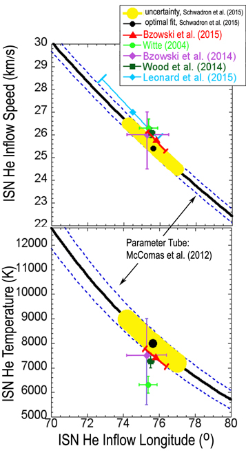
Figure 1. Top: relationship between  and the inflow longitude (
 ) according to the IBEX parameter tube based on various IBEX analyses in comparison with Ulysses results (adapted from Schwadron et al. 2015). Bottom: a similar relationship between the ISN temperature
  and the inflow longitude (
 ).
).
Download figure:
Standard image High-resolution image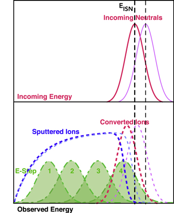
Figure 2. Schematic view of expected processed ion energy distributions of incoming neutral atom distributions (top) for direct conversion to negative ions (red dashed line) or sputtered ions (blue dashed lines). The IBEX-Lo E-Steps are indicated in green.
Download figure:
Standard image High-resolution imageThe ISN flow vector is one key parameter that determines the shape of the heliopause and the interaction of the interstellar plasma in the outer heliosheath with the ISN flow. The second key parameter is the local interstellar magnetic field direction, which is deduced from the orientation of the IBEX ribbon. Specifically, the local interstellar magnetic field direction is approximately at the center of the IBEX ribbon (Schwadron et al. 2009a). This field direction is roughly consistent with the heliospheric asymmetry found by the Voyagers (Opher et al. 2007; Pogorelov et al. 2009) and the TeV cosmic-ray anisotropy (Schwadron et al. 2014). In combination, the ISN flow and the magnetic field vector define the so-called B-V plane, which determines the symmetry plane of the outer heliosheath (e.g., Lallement et al. 2005; Schwadron et al. 2015, 2016). In addition, a debate about possibly detectable temporal variations of the ISN flow vector has started (Frisch et al. 2013, 2015; Lallement & Bertaux 2014). To detect such variations, or to place tight upper limits on them, requires the precise determination of the ISN flow vector over an extended time span of more than one solar cycle (at least a decade or more).
The needed independent information about the ISN flow longitude is derived from the characteristic ISN flow structures in the inner heliosphere, i.e., the gravitational focusing cone (Moebius et al. 1995; Gloeckler et al. 2004) and the crescent, both identifiable with PUI observations at 1 au (Drews et al. 2012). This independent information is remarkably resilient to solar wind structures and potential sensor efficiency variations, which have been eliminated in a careful statistical study by Drews et al. (2012). However, spatial and temporal variations of the ionization rate (Sokół et al. 2016) and PUI transport effects (Möbius 1996; Chalov 2006, 2014; Quinn et al. 2016) may lead to subtle deviations of the PUI spatial distribution relative to the parent neutral gas structures. More robust independent information may draw on the finding by Möbius et al. (1999) that the cutoff speed of the interstellar PUI distribution reflects the variation of the radial velocity component of the ISN flow at 1 au with ecliptic longitude and thus is an indicator of the ISN flow longitude.
In this study, we concentrate on the key observable of the ISN flow at 1 au on which the ISN parameter tube hinges most strongly. Namely, we focus on the ecliptic longitude λPeak that marks the maximum of the ISN flux as seen tangentially to Earth's orbit, which is uniquely related to the ISN bulk flow velocity that passes its perihelion at 1 au. The determination of λPeak can be obtained by evaluating the spin-integrated ISN fluxes, thus allowing the analysis with maximum counting statistics. A complication in the analysis is that the postacceleration voltage (PAC) was reduced and changed after discharge at the end of a very long spacecraft eclipse in 2012 July. We perform the analysis on spin-integrated ISN fluxes over the entire data set from 2013 through 2019, i.e., over 6 yr, and with energy steps 1–4 (15, 29, 55, 102 eV center energies) when the IBEX-Lo remained ∼7 kV. We use this analysis to provide an in-flight calibration of the relative IBEX-Lo efficiencies for the detection of He as a function of energy and testing the robustness of the method. Finally, we extend this method to determine the λPeak of the ISN flux for viewing elongations ηE > 90° from the Sun to explore the sensitivity of such observations to breaking the parameter degeneracy inherent in the ISN parameter tube. This exercise then provides a small preview of the capabilities of IMAP, which includes the ability to track the ISN flow over almost the entire orbit about the Sun (McComas et al. 2018; Sokół et al. 2019).
In Section 2 we briefly describe the instrumentation and mission, and the data selection. Extraction of the relative detection efficiencies and relative in-flight calibration for neutral He are described in Section 3. The results of the consolidated analysis are presented in Section 4, which is followed by the extension of the method to elongations >90° and its results in Section 5. The paper concludes in Section 6 with a discussion of these results, their implications for the ISN flow analysis, and a preview of how these results can be utilized with IMAP.
The paper also provides a series of appendices. Appendix A describes the frame-of-reference transforms applied to IBEX-Lo data. Appendix B describes the IBEX ISN parameter tubes. Appendix C describes the effect of secondary populations on the ISN parameter tubes.
2. Instrumentation, Mission, and Data Selection
The IBEX spacecraft was launched in 2008 October and subsequently rose into a highly elliptical Earth orbit with an apogee of about 50 RE. Its science goals are to discover the global interaction between the heliosphere and the ISM and to sample the neutral interstellar wind through the solar system. The IBEX viewing geometry provides for observation of the ISN atoms when they arrive nearly tangential to Earth's orbit, with high-enough energy when moving into the oncoming flow from late December through late March each year.
IBEX was designed to observe heliospheric and interstellar energetic neutral atoms (ENAs) with as little interference from terrestrial and magnetospheric backgrounds as possible. This Small Explorer (McComas et al. 2009a) carries two single-pixel high-sensitivity ENA cameras, IBEX-Hi (Funsten et al. 2009) and IBEX-Lo (Fuselier et al. 2009). Their fields of view (FoV) point radially outward in two opposite directions, and their combined energy range is 10–6000 eV with overlap between 300 and 2000 eV. IBEX is a roughly Sun-pointing, spinning satellite, whose spin axis is reoriented toward the Sun after completion of each 7–8 day orbit (2009–2011) and after each ≈4.5 day ascending and descending orbit arc after 2011 June (McComas et al. 2011). Complete full-sky ENA maps are obtained with the resolution of the 7° FWHM sensor FoV every six months. IBEX samples heliospheric and interstellar ENA distributions at 1 au in a plane that is approximately perpendicular to the Earth–Sun line. This is equivalent to observing these ENAs at the perihelia of their trajectories, independent of their flow direction at infinity.
2.1. IBEX-Lo Sensor
The IBEX-Lo sensor was optimized for the observation of the ISN gas flow of several species and for measuring ENAs in the energy range 10–2000 eV from the heliospheric boundary (Fuselier et al. 2009). IBEX-Lo uses a large-area collimator to define the 7° FWHM FoV. Negatively biased rejection rings and a positive potential at the collimator are designed to repel electrons and ions, allowing only neutral atoms and photons to enter the sensor. While electron rejection works as designed, the positive voltage cannot be applied to the collimator due to an anomaly that occurred during instrument commissioning in 2008 December. However, an additional internal deflection of incoming ions behind the IBEX-Lo collimator still prevents all ions with energies <200 eV from reaching the conversion surface, with partial rejection capability between 200 and 2000 eV. Neutral atoms (and ions >200 eV) that pass the collimator reach the conversion surface, where a small fraction is converted to negative ions. These negative ions are selected for energy/charge within eight logarithmically spaced energy steps by an electrostatic analyzer, which also rejects any neutrals and positive ions. Serrations and blackening of the analyzer surfaces efficiently suppress photons and secondary electrons (Wieser et al. 2007). After a +16 kV (+7 kV after 2012 July) postacceleration, negative ions are analyzed for their mass in a two-section time-of-flight (TOF) spectrometer. Triple-coincidence conditions very effectively reject nearly all background (Möbius et al. 2008, 2009).
The central electronics unit sorts the pulse height events based on their coincidence condition (giving triple-coincidence events the highest priority) and inserts a time tag (counting time from each spin pulse). Events identified as H and O by the TOF spectrometer are sorted into 6° bin-angle histograms for each energy step (for details, see Fuselier et al. 2009).
The IBEX-Lo TOF spectrometer determines the mass of incoming neutral atoms directly for species (e.g., H and O) that are converted to negative ions. Noble gases, such as He and Ne, produce few, if any, converted negative ions (Smirnov & Massey 1982), but generate sputtered negative ions (H, C, and O) from the conversion surface. These sputtered negative ions are detected and identified in the IBEX-Lo TOF spectrometer (Wurz et al. 2008; Möbius et al. 2009). The IBEX-Lo sensor was calibrated in the laboratory for its response using He and Ne at a variety of energies (Fuselier et al. 2009; Möbius et al. 2009). The observed ratios of H, C, and O provide an observational signature used to infer the identity of the parent noble gas atom (He or Ne), here relevant for ISN He. Sputtered ions generate a broad energy distribution that cannot exceed the incoming energy of the neutral atom and extends to very low energies (Möbius et al. 2012), which results in a flat energy response to the He ISN flow distribution (see Figure 2). However, sputtering has a low-energy cutoff that is relevant for potential IBEX-Lo observations of the ISN flow during fall, when the spacecraft and Earth recede from the ISN flow (Galli et al. 2015; Sokół et al. 2015) and for low-energy atoms from the Warm Breeze (Kubiak et al. 2014). The Warm Breeze is a secondary neutral atom population created through charge exchange within the modified LISM, and this secondary population is warmer, slower, and deflected with respect to the primary ISN flow.
2.2. Data Selection
The selection of the interstellar gas flow observations for analysis follows the same criteria described in Möbius et al. (2012), which we briefly summarize. An ISN list is generated for each ISN flow season that is the basis for the data selection and analysis. Excluded from this list are time periods, when any of the following conditions apply:
- 1.IBEX is close to the magnetosphere and IBEX-Lo observes significant count rates of magnetospheric ENAs and ions, based on observations away from the ISN flow.
- 2.The Moon is in the IBEX FoV. These times are taken from the ISOC command files, which contain special commanding for the star sensor during these times.
- 3.The electron rates for IBEX-Lo are high. These times are identified in the IBEX-Lo TOF count rates, when the otherwise very stable base count rate outside the ISN flow direction is exceeded by more than a factor of 1.6 (safely above any stochastic fluctuations of the base count rate, but low enough to indicate significant increases). This criterion independently eliminates any time periods with contamination by magnetospheric ENAs, which led to similar rate increases.
- 4.The star tracker function has been impaired by bright sources, such as Earth or the Moon near its FoV. This affects the precise determination of the ISN peak location and width in latitude and thus is excluded from the analysis.
In addition to the ISN list, a"good times" list is used to capture the time periods with very low background rates.
In a first analysis step, we fit the angular ISN flow distributions obtained within each orbit or orbit arc to a Gaussian distribution, which includes an adjustable constant background as one of the parameters. The level of this background is typically <1/450 or at least <1/125 of the peak rate (Leonard et al. 2015). This level ensures that any background is at most a small contribution to the apparent ISN flow signal.
We exclude observations at ecliptic longitudes λObs < 115° (IBEX orbits equivalent to orbit 13 or lower in 2009) and ecliptic longitude λObs > 160° (IBEX orbits equivalent to orbit 20 or higher in 2009) from the ISN flow vector analysis. The former condition minimizes the influence of the Warm Breeze on the results. Because of the importance of the Warm Breeze influence and its apparently different impact on flow peak location and width, we discuss its effects in more detail in Sections 3 and 4. The latter condition also renders a negligible influence from the H ISN flow (Saul et al. 2012; Schwadron et al. 2013) on the He observations.
Complete ISN flow analysis (Bzowski et al. 2012; Möbius et al. 2012; Bzowski et al. 2015; Swaczyna et al. 2015; Schwadron et al. 2015) requires detailed model comparisons to spin-phase distributions, which in turn rely on precise pointing and spin-phase information. In contrast, the observations used in this paper draw from spin-integrated count rates and therefore do not require high-precision pointing. We therefore are able to include observation times when the IBEX star tracker was not functioning nominally and the observations are "despun," i.e., viewing directions are corrected on the ground (McComas et al. 2012b, 2014).
3. Relative In-flight Calibration for Neutral He
Accurate calibration of the observing instrument (IBEX-Lo, and IMAP-Lo) is extremely important when it comes to precision measurements, as, for example, in the determination of the interstellar flow vector. To obtain the interstellar flow vector from the IBEX observations, the ISN flow distribution has to be compiled for different observing locations in longitude along Earth's orbit and different pointings in latitude (Möbius et al. 2012, 2015b; Bzowski et al. 2012, 2015; Schwadron et al. 2015). Because the mean energy of the neutral atom distributions in the observer frame varies with these observing conditions, any dependence of the IBEX-Lo efficiency on energy will influence the resulting ISN flow vector.
A precise relative calibration for the energy dependence of the instrument efficiency is needed for the analysis of the ISN flow distribution to obtain the flow vector and temperature. We resort to a method that makes use of the ISN flow at 1 au as a stable neutral atom beam for in-flight calibration. This does not require knowledge of the absolute flux or any absolute collection efficiency. Here we perform an analysis of the IBEX-Lo He ISN flow observations that does not require knowledge of the detailed ISN flow distribution. We use the spin-integrated ISN flow signal obtained in each orbit. All that is needed in this scheme is the mean energy (or bulk flow speed) of the atom distribution collected in each orbit.
Figure 16 is adapted from Möbius et al. (2012) and shows schematically how incoming neutral atoms are processed by the IBEX-Lo sensor for detection via conversion of neutrals to negative ions and via sputtering. The conversion process produces an ion distribution with a somewhat-reduced mean energy (∼10%–20%; Fuselier et al. 2009) but which is still rather narrow. In contrast, sputtering produces a broad ion distribution with energies down to almost 0 eV and a sharp cutoff noticeably below the incoming energy. For ISN He the incoming mean energy in the spacecraft frame is at ∼120–140 eV, or still substantially above the center energy of IBEX-Lo E-Step 4 (110 eV for H–) (Fuselier et al. 2009; Möbius et al. 2009). Therefore, comparable sputtered H– count rates are collected in E-Steps 1–3 and substantially reduced count rates in E-Step 4 because its center energy is close to the cutoff of the sputtered distribution. The distributions shown with thinner lines indicate the expected change of the instrument response to input at higher energies: the count rates in E-Step 4 will likely increase substantially, while those in E-Step 1 and 2 may decrease slightly and E-Step 3 is likely affected the least because the sputtered distribution broadens in energy with the incoming flow.
The mean energy of the ISN flow distribution collected as a function of ecliptic longitude is needed to determine the variation of the instrument response with incoming neutral energy in all four energy steps. The peak of the ISN flow distribution observed exactly at perihelion is associated with ISN trajectories that arrive centered exactly perpendicular to the spacecraft–Sun line. The energy of this perihelion peak is determined analytically as a function of ecliptic longitude (Lee et al. 2012; Möbius et al. 2012) for a given ISN flow vector. We apply this relation for the values from the 2015 analysis  km s−1 and
  (McComas et al. 2015b). Even a ±1 km s−1 uncertainty in the ISN flow speed outside the heliosphere creates only a small ±1.25% uncertainty in the flow speed
  observed in the spacecraft frame:

because of the large contribution of the precisely known speed of the Earth VE to the observed speed  . Atoms arriving from angles slightly out of the ecliptic gain slightly less speed from the frame transformation. This slightly reduces the observed peak flow speed. Because the ISN flow arrives with
  and the thermal σ width of the observed ISN He flow at 1 au is 5
 5–9° over the observation of the primary ISN flow (Möbius et al. 2015b), these reductions are 0.15% due to average out-of-ecliptic motion and 0.13%–0.45% due to the thermal σ width. These reductions are much smaller than the uncertainty of the flow speed and are ignored here.
We are interested in a relative calibration of the IBEX-Lo energy response. We therefore consider ratios of the observed count rates in E-Steps 1–4. Based on the behavior of the sputtered ion distribution (Figure 16), we use the rates in E-Step 3 as the denominator. Figure 3 shows the respective ratios for E-Steps 1, 2, and 4 as a function of the incoming energy of the ISN flow  in the IBEX frame for the observation intervals of the primary ISN He flow for 2009–2012 (left, PAC = 16 kV) and 2013–2019 (right, PAC = 7 kV). The change in the PAC voltage accounts for the shift in the energy dependence observed before and after the start of 2013. Specifically, while the ratios for E-Steps 1 and 2 decrease slightly with the ISN flow energy after 2013, the ratio for E-Step 4 increases, as suggested in Figure 16. The increase in E-Step 4 over the accessible ISN energy range amounts to almost a factor of 2 due to the lower count rate (by approximately a factor of 5 over the other E-Steps).
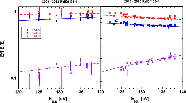
Figure 3. Efficiencies for energy steps 1, 2, and 4 relative to energy step 3 are shown as a function of the energy of primary interstellar neutral He. The left panels apply for 2009–2012 when the PAC = 16 kV, and the right panels apply for 2013 and after when the PAC = 7 kV. Therefore, we separate the analysis of relative efficiencies before and after the PAC change. We have culled the data for periods where the primary He interstellar neutral atoms are dominant (specifically we use the criterion that WB/ISN < 0.01, where WB corresponds to the He Warm Breeze rates and ISN corresponds to the primary ISN He rates.
Download figure:
Standard image High-resolution imageWe present the energy dependence of the response of all four IBEX-Lo E-Steps in a format that is guided by the schematic (Figure 16). We normalize the center energies Ei
(i = 1–4) of these E-Steps to the mean energy of the observed ISN He distribution  for each observation. Figure 4 shows the ratios of the count rates of E-Step i over E-Step 3, which we now identify as the relative efficiencies Eff(Ratei
/Rate3) as a function of the normalized energies
for each observation. Figure 4 shows the ratios of the count rates of E-Step i over E-Step 3, which we now identify as the relative efficiencies Eff(Ratei
/Rate3) as a function of the normalized energies  . Separately shown are data from the first 4 yr (2009–2012) in blue and thereafter (2013–2018) in red. Also shown are two chi-squared fits to an analytical curve that smoothly connects the energy ranges covered by all four E-Steps and is reminiscent of the schematic behavior indicated in Figure 16. As a heuristic fitting function for the rate ratios in Figure 4, we adopt the following:

where y = Ri
/R3 is the count rates in each energy step normalized to that of energy step 3 and  is the center energy of the energy step of interest normalized to the mean energy of the ISN flow distribution that is observed.
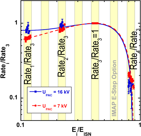
Figure 4. Ratios of spin-integrated count rates (Ratei
/Rate3), where i = 1, 2, 4 as a function of the ratio of the center energy of the E-Step over the mean ISN energy in the S/C frame ( ) for postacceleration voltages of 16 kV (2009–2012, blue) and 7 kV (≥2013, red). The yellow bars indicate optional finer E-Steps with IMAP-Lo.
Download figure:
Standard image High-resolution imageThe relative efficiencies remain stable over the years of the IBEX-Lo operations, with only one visible change between 2012 and 2013 due to the reduction of the PAC voltage. As in Figure 3, the efficiencies decrease with increasing  for E-Steps 1 and 2 but increase strongly for E-Step 4. The relative efficiency is pegged at 1 for E-Step 3 because we use the count rate in E-Step 3 as the denominator. The center energy of E-Step 3 appears to be closest to the maximum of the efficiency curve. Whether it is at the maximum or the efficiency is slightly increasing or decreasing with ISN flow energy cannot be determined with the sparsely distributed E-Steps. The energy dependence in E-Steps 1 and 2 grew stronger after the PAC voltage reduction.
The steeper variation of the efficiency with energy in E-Steps 1 and 2 after the PAC reduction may be connected to the two different populations of sputtered particles that are generated. So-called knock-on sputtering occurs as an encounter of a He atom with a single surface atom (or molecule) and typically results in sputter products with higher energies concentrated in angle around the specular reflection of the incoming ISN atom on the conversion surface. Sputtering due to excitation of the surface lattice leads to boil-off of atoms with very low energy and with an almost isotropic angular distribution (Sigmund 1981). The focusing of the angular distribution of ions from the conversion surface and thus the effective collection of these ions improves with increasing PAC voltage (Wieser et al.2007).
Figure 4 demonstrates that the variation of the efficiency with incoming ISN flow energy is very small for E-Steps 1–2, and it is almost completely absent for E-Step 3. We test for the consequences of this behavior by performing our data analysis for all four E-Steps first and then continue our analysis with E-Step 3, which appears to be least sensitive to variations with energy.
The observations of the neutral atom fluxes are taken in the spacecraft frame, while the ISN flow distribution is ultimately evaluated either in the inertial frame or in the Earth frame. In the latter two frames, a coherent description of the distribution is possible, while the state of motion of the spacecraft that affects the observed fluxes and their incoming directions changes periodically over each orbit. The transformation between the inertial frame and the Earth frame is already built into the analytic model of the ISN flow (Lee et al. 2012, 2015). Therefore, we transform the observed fluxes into the Earth frame before performing an analysis with the ISN flow distribution.
4. ISN Parameter Tube for Multiple Energy Steps and Observations from 2013–2019
The determination of the ecliptic longitude λPeak of the ISN flow peak can be used to deduce a narrowly constrained parameter tube that is characterized by a functional relation between  and
and  based on the hyperbolic trajectory equation (Lee et al. 2012; Möbius et al. 2012; McComas et al. 2012a). Therefore, the maximum of the ISN flux λPeak is a key observable of the IBEX measurements that enters strongly into the determination of the ISN flow parameters. In the following, we consolidate the ISN flow peak observations for energy steps 1 through 4 (with central energies 15, 29, 55, and 102 eV), in which the signal of the He ISN flow is observed, and we combine all available observation seasons with comparable measurement conditions. We combine the observations for 2013 through 2019 here and exclude earlier periods because the IBEX-Lo count rates of the He ISN flow were reduced noticeably during the first three years of IBEX-Lo operations. This reduction was caused by the competition of electron-related events for the limited bit rate capability across the IBEX-Lo interface (Möbius et al. 2012; Swaczyna et al. 2015). The effect was subsequently eliminated through an onboard scheme to isolate electron-related events and remove them from telemetry prior to transmission across the IBEX-Lo interface. In addition, the postacceleration voltage was reduced in 2012 (Möbius et al. 2015a); after July, 2012 the PAC voltage remained stable.
The spin-integrated IBEX-Lo count rates of each year were adjusted individually for
- 1.transformation between the spacecraft reference frame and the Earth frame (Appendix A),
- 2.contribution of secondary neutral He to the observed count rates,
- 3.conversion from energy flux density (proportional to count rates) to phase-space density (PSD), and
- 4.ionization loss of the ISN He along their trajectories to the observer.
The first three adjustments are performed directly on the observed ISN He count rates, while the last adjustment concerns the original neutral gas density as a function of location in the heliosphere and thus must be applied to the PSD.
As detailed in Section 3, the sputtered rates in E-Step 3 provide the most reliable assessment of ISN parameters. Compared to E-Step 3, the sputtered rates in E-Step 4 are sharply lower because the high-energy sputtering cutoff occurs at or below this energy step. The rates in E-Step 2 and E-Step 1 are also lower than those in E-Step 3 after the lowering of the PAC voltage (2013 and beyond). Therefore, E-Step 3 (central energy 55 eV) provides the most direct response to the primary He population because its energy is slightly lower than but close to the incident energy of primary interstellar He atoms.
The transformation of the observed rates into the Earth reference frame (see Appendix A) is performed on the raw data, before averaging is applied, because it varies with the spacecraft velocity vector as a function of position in each individual IBEX orbit. The spin-integrated count rates are observed over a varying ecliptic pointing angle  E
, defined as the instantaneous angle between the spin axis relative to the Earth–Sun line (Figure 5). This figure also shows the elongation angle ηE
, defined as the angle between the Earth–Sun line and the IBEX-Lo boresight. The rates show clear monotonic trends, allowing us to interpolate or extrapolate to fixed values of E
, as exemplified in Figure 6. If the amount of extrapolation that is needed to arrive at the desired fixed value of E
exceeds the extent of the angle range of the available data for an orbit arc, then this arc is eliminated from further analysis.
E
, defined as the instantaneous angle between the spin axis relative to the Earth–Sun line (Figure 5). This figure also shows the elongation angle ηE
, defined as the angle between the Earth–Sun line and the IBEX-Lo boresight. The rates show clear monotonic trends, allowing us to interpolate or extrapolate to fixed values of E
, as exemplified in Figure 6. If the amount of extrapolation that is needed to arrive at the desired fixed value of E
exceeds the extent of the angle range of the available data for an orbit arc, then this arc is eliminated from further analysis.
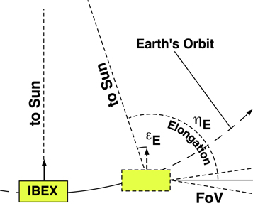
Figure 5. Westward drift of the pointing of the IBEX spin axis E
and of the IBEX-Lo FoV (elongation angle) ηE
over the course of an orbit or orbit arc relative to the Sun. Two positions (not to scale) of IBEX are shown for illustration, at the point of Sun-pointing and at a point where the spin axis has moved to a positive ecliptic spin-axis angle E
. Both angles E
and ηE
are projected and calculated within the ecliptic plane.
Download figure:
Standard image High-resolution image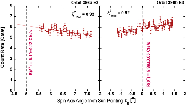
Figure 6. Spin-integrated count rates as a function of spin-axis pointing for orbit 396, arcs a (left) and b (right). Orbit 396b is an example of an orbit in which the spin-axis angle rotated through Sun-pointing, which is the nominal case for IBEX in most orbits or orbit arcs. Orbit 396a is a case where the spacecraft spin axis was intentionally directed to larger spin-axis angles E
. The lines show fits to the observed spin-integrated count rates, and the derived rates at E
= 0° and E
= 5° are shown.
Download figure:
Standard image High-resolution imageThe IBEX observations are made in a frame of reference that is moving with respect to the Sun both due to Earth's motion about the Sun, and the spacecraft motion about Earth. Multiple transformations are used to correct for effects associated with the IBEX moving frame of reference and to compare observations in the inertial reference frame. Appendix A.3 details the shift in longitudinal position associated with the moving reference frame. We correct for this shift to determine an "aberrated longitude," a position where the velocity of an atom in the spacecraft frame has no component in the radial direction. This shift in longitude represents purely a positional translation and does not affect the velocity vector of incident atoms.
The contribution of secondary neutral He to the observed ISN He signal is determined as an integral value in each orbit. These contributing secondary rates are computed in simulations according to Kubiak et al. (2014, 2016). The secondary rates are typically large for early orbits in each season and higher for years near solar minimum conditions. We remove from analysis orbits where secondary contributions exceed 20% (this is the largest percentage for the secondary neutral contribution in which the primary population is dominant, and the secondary component can be treated as a small correction). For all remaining orbits the secondary neutral contribution is subtracted from the observed rates.
The rates are adjusted for the fact that the bulk flow peak must be determined as the peak in ISN He PSD. We define a PSD-corrected rate and use it henceforth so that we can continue to use the rate-based unit (counts s−1) for direct comparison. Finally, we adjust these PSD-corrected rates for the ionization loss using the ionization rates based on Sokół et al. (2020). In order to stay with the analytic approach, we use the average over the 6 months prior to the orbit of interest, which is approximately equivalent to the transit time of the ISN atoms from 3.15 au to 1 au, i.e., starting where ionization loss amounts to 10% of its value at 1 au as a fixed input value. We include the estimated total ionization rate, with the approximation that ionization rates vary as 1/r2, which is correct for the dominant rates, photoionization, and charge exchange, while the small contribution (outside 1 au) of electron-impact ionization deviates from this inverse square radial dependence.
Figure 7 shows the PSD-corrected spin-integrated ISN He rates of 2013–2019 combined for energy steps 1 through 4, after the adjustments indicated previously. Also shown are the χ2 fits to a Gaussian distribution in ecliptic longitude, along with the resulting values and fit errors for λPeak. Individual data points have scatter with respect to the fit curve that are consistent with normal Poisson fluctuations. The resulting values for λPeak are almost identical for energy steps 1 through 3 within the combined error bar for each pair of the values. However, for energy step 4, λPeak is significantly larger compared with the other three values outside their mutual 1σ error bars.
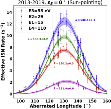
Figure 7. Spin-integrated count rates of the He ISN flow, obtained in E-Steps 1–4 at the location of exact Sun-pointing of the IBEX spin axis, corrected for aberration. The count rates have been transformed from flux to phase-space density and adjusted for ionization loss and the presence of secondary He. Also shown are the chi-squared fits to a Gaussian with the resulting peak longitudes.
Download figure:
Standard image High-resolution imageThis trend of λPeak is reemphasized in Figure 8, which shows λPeak as a function of the center energy of the four energy steps in which ISN He is observed. The dashed–dotted horizontal line indicates the weighted average value of λPeak for the first three energy steps, and the dashed vertical line represents the bulk energy of the ISN He flow in the spacecraft frame at λPeak.
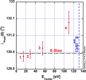
Figure 8. Peak longitudes λPeak with fit error bars as a function of E-Step energy. The dashed–dotted horizontal line shows the inverse-variance-weighted average value for the first three energy steps (λPeak = 13029 ± 015), and the dashed vertical line shows the ISN He bulk flow energy in the spacecraft frame.
Download figure:
Standard image High-resolution imageThe behavior of λPeak as a function of the center energy of each energy step can be understood as the response to the energy dependence of the IBEX-Lo detection efficiency (Section 3). As is evident from Figure 4, the efficiency increases only slightly with the ratio  for the entire range of the ISN flow observations for E-Steps 1 and 2 and is almost exactly flat for E-Step 3. However, for E-Step 4, which has an energy only ∼25% below the ISN bulk energy, this efficiency ratio decreases sharply by almost a factor of 2 over the relevant observation range.
Note that the energy of the ISN flow generally decreases with observer longitude as a result of gravitational focusing. Therefore, efficiency changes as a function of energy cause a small bias with observer longitude. The sensor efficiency decreases very slightly with observer longitude for E-Steps 1 and 2, stays constant for E-Step 3, and increases noticeably for E-Step 4. As a result, the observed count rates of the ISN flow are either very slightly reduced or noticeably increased (for E-Step 4) at larger observer longitudes. The very slight change in the lowest energy steps is within the statistical error bars, while the efficiency variation in E-Step 4 skews the longitudinal distribution of the observed count rates so that the resulting peak values move to larger longitude. Because the efficiency is flat for E-Step 3 and the rates in this step are the highest of the four relevant energy steps we focus on this energy step for further analysis.
5. Breaking Parameter Degeneracy through Observations from Different Ecliptic Longitudes
For the analytic evaluation of the ISN He flow observations, we have interpolated or extrapolated the IBEX-Lo observations to the ecliptic longitude where the IBEX spin axis points exactly to the Sun in the ecliptic plane (E
= 0° and ηE
= 90°) (Möbius et al. 2012, 2015a). If this condition is met for the maximum of the ISN flow, then the ISN bulk flow trajectory is observed at its perihelion at 1 au. This is the observation condition that defined the ISN parameter tube and the degeneracy along the function (Lee et al. 2012; Möbius et al.2012; McComas et al. 2012a) .
If the ISN bulk flow is observed over a variety of ecliptic longitudes, then this parameter degeneracy is broken. This principle was, for example, demonstrated with the Ulysses-GAS ISN He observations (Bzowski et al. 2014; Wood et al. 2015). In Earth orbit, however, breaking the degeneracy requires the capability to point the instrument FoV at elongations ηE
from the Sun that deviate substantially from the nominal IBEX orientation shown in Figure 5. This capability is designed into the upcoming Interstellar Mapping and Acceleration Probe (IMAP) mission (McComas et al. 2018) and is the subject of current science planning (Sokół et al. 2019). With the westward drift of the IBEX spin axis over the course of each orbit (or orbit arc after 2011), as indicated in Figure 5, IBEX provides observations with small deviations up to E
= + 7° (or up to elongations of ηE
= 97°). We use these deviations to demonstrate the principle and provide the first broken degeneracy in the ISN parameter tube for IBEX.
Larger elongations >90° capture ISN flow trajectories before the ISN atoms have reached their perihelion because at 1 au, they are still moving toward the Sun. In analogy to the procedure in the previous section, we determine the ecliptic longitude of the ISN flow peak for ηE > 90°. We simply obtain the count rates for a range of elongations by interpolation or extrapolation, applying the same conditions that we used in Section 4 for ηE = 90°. Of course, different orbits (arcs) may be eliminated from analysis or added to the analysis depending on the range of ηE covered with the good times selection for each orbit (arc).
Figures 9 and 10 show the ISN He count rates in energy steps 1–4 for E
= 2° (ηE
= 92°, Figure 9) and for E
= 5° (ηE
= 95°, Figure 10). As expected, the flow maximum for ηE
= 92° and ηE
= 95° is shifted to larger longitudes, by ∼5° and ∼12°, respectively.
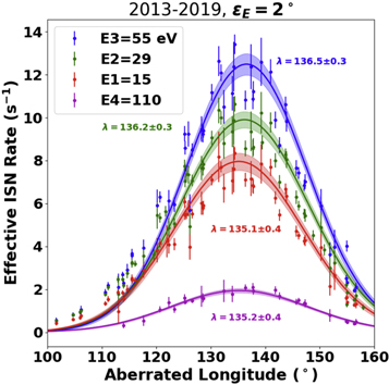
Figure 9. Spin-integrated count rates of the He ISN flow, obtained in E-Steps 1–4 at the location of the E
= 2° off-pointing of the IBEX spin axis, corrected for aberration. The count rates have been transformed from flux to phase-space density and adjusted for ionization loss and the presence of secondary He. Also shown are the chi-squared fits to a Gaussian with the resulting peak longitudes.
Download figure:
Standard image High-resolution image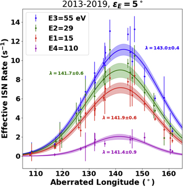
Figure 10. Spin-integrated count rates of the He ISN flow, obtained in E-Steps 1–4 at the location of the E
= 5° off-pointing of the IBEX spin axis, corrected for aberration. The count rates have been transformed from flux to phase-space density and adjusted for ionization loss and the presence of secondary He. Also shown are the chi-squared fits to a Gaussian with the resulting peak longitudes.
Download figure:
Standard image High-resolution imageFigure 11 shows the resulting λPeak values and errors for the distributions shown in Figures 8–10 (ηE
= 90°, 92°, and 95°). Also shown are the analytic curves for the parameter tube detailed in Appendix B, computed for the following ISN reference velocity vector:  km s−1,
  , and
, and  . These parameters were derived as inverse-variance-weighted averages of previous ISN parameter determinations, as listed in Table 1.
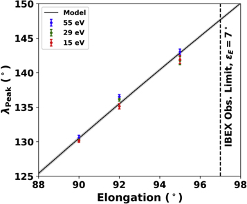
Figure 11. Ecliptic longitude of the ISN flow peak λPeak as a function of elongation ηE in the heliocentric reference frame, based on observations (see Figures 8–10) and on analytic modeling for the ISN parameter tubes (Appendix B).
Download figure:
Standard image High-resolution imageTable 1. Local Interstellar Conditions
| Method/instrument |

|

|

|

| Reference |
|---|---|---|---|---|---|
| (km s−1) | (deg) | (deg) | (K) | ||
| Neutral Gas/Ulysses-GAS | 26.3 ± 0.4 | 75.4 ± 0.5 | −5.2 ± 0.2 | 6300 ± 340 | Witte (2004) |
| Neutral Gas/Ulysses-GAS | 26.08 ± 0.21 | 75.54 ± 0.19 | −5.44 ± 0.24 | 7260 ± 270 | Wood et al. (2015) |
| Neutral Gas/Ulysses-GAS | 26 | 75.30 | 7500 | Bzowski et al. (2014) | |
| Neutral He/IBEX | 25.4 | 75.7 | −5.1 | 7500 | McComas et al. (2015a) |
| Neutral He/IBEX | 25.8 ± 0.4 | 75.8 ± 0.5 | −5.16 ± 0.1 | 7440 ± 260 | Bzowski et al. (2015) |
| Neutral He/IBEX a |

|

| −
|

| Schwadron et al. (2015) |
| Neutral He/IBEX | 25.82 ± 0.33 | 75.62 ± 0.36 | −5.19 ± 0.06 | 7673 ± 225 | Swaczyna et al. (2018) |
| UV backscatter/EUVE | 24.5 ± 2 | 74.7 ± 0.5 | −5.7 ± 0.5 | 6500 ± 2000 | Vallerga et al. (2004) |
| UV backscatter/Prognoz 6 | 74.5 ± 1 | −6 ± 1 | Lallement et al. (2004) | ||
| Pickup Ions/ACE-SWICS | 74.43 ± 0.33 | Gloeckler et al. (2004) | |||
| Pickup Ions/STEREO-PLASTIC | 75.41 ± 0.34 | Taut et al. (2018) | |||
| Average b | 25.99 ± 0.18 | 75.28 ± 0.13 | −5.200 ± 0.075 | 7496 ± 172 | This study |
| Param Tube Intersection c |

|

| −
|

| This study |
| Absorption/Haute-provence | 25.7 ± 1 c | 7000 ± 1000 d | Lallement & Bertin (1992) | ||
| Absorption/Hubble | 7000 ± 200 d | Linsky et al. (1993) | |||
Notes.
a We state both fit uncertainties (in superscript) and the total uncertainty (in subscript). The total uncertainty is the rms sum of the fit and statistical and systematic uncertainties. b Averaging is done using inverse variance weighting with independent values where available, including results from Wood et al. (2015), Swaczyna et al. (2018), Vallerga et al. (2004), Lallement et al. (2004), Gloeckler et al. (2004), and Taut et al. (2018). We exclude the bottom two rows that apply to the local interstellar cloud. c Intersection in parameter tubes provides an outer range of uncertainties associated with longitudinal inflow direction and ISN He bulk flow speed. We use similar relations detailed by McComas et al. (2012b) to derive uncertainties for temperature and latitudinal inflow direction
  along the parameter tube:
  , and
, and  .
d
Local interstellar cloud bulk parameters.
.
d
Local interstellar cloud bulk parameters.Download table as: ASCIITypeset image
In Table 1, we use information from IBEX and other observatories to reduce parameter uncertainties. These uncertainties are smallest across the parameter tube, but the degeneracy in IBEX measurements remains along the 4D parameter tube. This indicates that the reductions in the parameter uncertainties can be used in this case of IBEX to reduce the width of the parameter tube. The crossing of independent parameter tubes measured from differing elongations are used to limit systematic uncertainties.
The argument in this case depends not only on IBEX measurements (Bzowski et al. 2015; McComas et al. 2015a; Schwadron et al. 2015; Swaczyna et al. 2018) but also on those from Ulysses measurements of the neutral gas (Witte 2004; Bzowski et al. 2014; Wood et al. 2015), PUIs (Gloeckler et al. 2004; Taut et al. 2018) and UV backscatter (Lallement et al. 2004; Vallerga et al. 2004). Each of these determinations suffers from potential systematic uncertainties, as detailed in the discussion and conclusions. Therefore, the additional constraints imposed by crossing parameter tubes at different elongations become critical for rendering a determination with limited systematic uncertainties.
The reference ISN parameters exist as a point along the 4D functional parameter tube, as detailed in Appendix B. The inflow speed and inflow latitude direction are described along a smooth function of the inflow longitude direction. Figure 12 shows the functional tubes at the three measured elongations (90° in red, 92° in green and 95° in blue). The black dashed lines (top panel) indicate the reference ISN parameters  and V = 25.99 km s−1 where the parameter tubes cross. The shaded regions indicate the 1σ uncertainties. We observe that the distinct elongations measured by IBEX only weakly break the degeneracy in the parameter tubes because the angle between them is relatively small. Given the uncertainty across the parameter tubes, the range of possible inflow longitude directions is over the range
  .
.
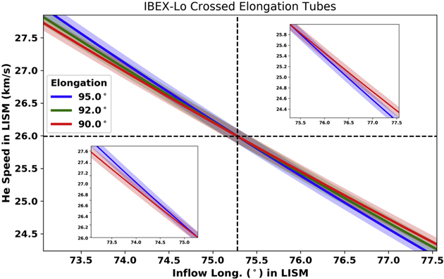
Figure 12. Following λPeak with different elongations ηE
from the Sun provides different ISN parameter tubes using the relations in Appendix B. Shown here are the range of elongations and associated parameter tubes accessible with IBEX. Insets show the left and right regions of parameter tube crossings. The range of possible inflow longitudes extends over  for the weakly crossed parameter tubes observed by IBEX.
Download figure:
Standard image High-resolution imageAs a way to check the consistency of the parameter determination, we also analyze the variation in the peak latitude of the bulk ISN flow, as shown in Figure 13. In this part of the study, we determine the peak latitude in the spacecraft reference frame and forward-model parameter tubes. We obtain the count rates in the spacecraft frame for a range of elongations, again applying the conditions that we used in Section 4 for ηE
= 90°. In this case, we exclude orbit arcs with extrapolations, and instead of interpolating for a specific ecliptic longitude, we average elongations for a specific array of orbits chosen. Table 2 indicates the average elongations and corresponding orbit arcs for each of these cases. It is notable that there are two cases associated with intermediate off-pointing, E
∼ 2°: cases A and B occur before and after orbit 316, respectively. As detailed in the next paragraph, orbit 316 marks an important change in the spacecraft spin-phase binning, and the spin angles before and after orbit 316 need to be treated separately.
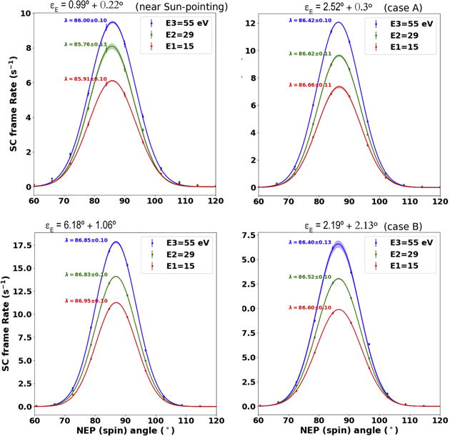
Figure 13. Count rates of the He ISN flow in the spacecraft reference frame as a function of the spin angle (angle from north-ecliptic pole, NEP), obtained in E-Steps 1–3 for ecliptic spin-axis angles: E
= 0.99 ± 0.22 (top left) from orbit arcs 234b and 274b; E
= 2.52 ± 0.30 (top right) from orbit arcs 195b, 235a, and 235b; = 2.19 ± 2.13 (bottom right) from orbit 355b; and E
= 6.18 ± 1.06 (bottom left) from orbit arcs 356b and 397a. Also shown are the chi-squared fits to a Gaussian with the resulting peak latitudes.
Download figure:
Standard image High-resolution imageTable 2. Average Elongations and Corresponding Orbit Arcs for Each of These Cases
| ηE (deg) a | Case | Orbit Arcs |
|---|---|---|
| 90.99 ± 0.22 |
E
∼ 0°, Near Sun-pointing | 234b, 274b |
| 92.52 ± 0.30 |
E
∼ 2°, Case A | 195b, 235a, 235b |
| 92.19 ± 2.13 |
E
∼ 2°, Case B | 355b |
| 96.18 ± 1.06 |
E
∼ 5°, Max off-Sun-pointing | 356b, 397a |
Note.
a The uncertainty range of ηE covers the full range of elongation angles over the period from which observations were used.Download table as: ASCIITypeset image
For orbit arcs 316a and beyond, a correction was made to account for a systematic shift in the spin angle between the boresight direction and the north-ecliptic pole (NEP angle). Recent analysis (Swaczyna et al. 2021) confirms that the observations after the star tracker anomaly in orbit arc 315b (as a consequence, the star tracker remained off for most of the time between orbits 316 and 326) show a systematic shift in the NEP angle of 06 compared to the observation before the anomaly. This is in agreement with the results obtained from the preliminary ISN analysis. Consequently, analyses of the ISN data should account for the shift of 06. While the star sensor data do not allow for independent determination of the spacecraft orientation for most orbits, they allow for the confirmation of q systematic shift with a precision of ∼01.
Model results are taken in the spacecraft frame and averaged over the spacecraft velocities for each interval. Figure 14 shows the model results compared to observations. Analytic curves for the parameter tube, as detailed in Appendix B, are computed for the following ISN reference velocity vector (see Table 1):  km s−1,
  ,
,  . Based on Appendix C, we include the secondary population and use results from Kubiak et al. (2016) with longitude 7157, latitude −1195, and speed 11.28 km s−1. Note in this case, because the rates are taken in the spacecraft reference frame (rather than in Earth's reference frame, as discussed in Section 4), the model must include spacecraft motion. The somewhat jagged model averages result from changes in the spacecraft motion for the specific orbit intervals used over a given elongation.
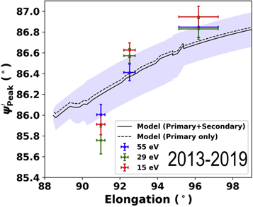
Figure 14. Ecliptic latitude of the ISN flow peak  in the spacecraft frame as a function of elongation ηE
, based on observations (see Figure 13) and on analytic modeling for the ISN parameter tubes (Appendix B) and including secondary populations (Appendix C). We show both model results including primary and secondary populations (solid curve) and including only the primary population. The model curves represent averages over the regions analyzed. The shaded region shows the range of variation associated primarily with spacecraft motion and additional uncertainties in the parameter tube. For E-Step 3 (blue points), the model predictions generally agree with observations within the 1σ uncertainty intervals and over at least a portion of the region associated with spacecraft motion (blue shaded region).
in the spacecraft frame as a function of elongation ηE
, based on observations (see Figure 13) and on analytic modeling for the ISN parameter tubes (Appendix B) and including secondary populations (Appendix C). We show both model results including primary and secondary populations (solid curve) and including only the primary population. The model curves represent averages over the regions analyzed. The shaded region shows the range of variation associated primarily with spacecraft motion and additional uncertainties in the parameter tube. For E-Step 3 (blue points), the model predictions generally agree with observations within the 1σ uncertainty intervals and over at least a portion of the region associated with spacecraft motion (blue shaded region).
Download figure:
Standard image High-resolution imageThe E-Step 3 observations (blue points) agree with model predictions within the 1σ uncertainties. As detailed in Section 3, E-Step 3 count rates provide the best estimate for the variation in count rates as a function of elongation. The model and observations consistently show an increase in the peak latitude with increasing elongation angle. However, the latitude peak increase is quite small (∼1°) over the range of elongations used for analysis. The model is consistent with observations, but in addition to the longitude peak (see Figure 11), the observed latitude peak (see, Figure 14) provides relatively little additional statistical leverage to reduce the parameter degeneracy.
6. Discussion and Conclusions
IBEX observations over more than a decade have revealed a consistent velocity and temperature of the local interstellar flow based on observations of the primary ISN He population. IBEX observations are made over a distinct region of space where measured neutral atoms reach almost their perihelion along their trajectories and oppose Earth's motion around the Sun. At this point along the ISN He trajectories, the energy of incident atoms is maximized in the spacecraft frame, which enhances statistics and reduces uncertainties. The measurement though is paired with a degenerate parameter set, which is known as the IBEX 4D parameter tube (Lee et al. 2012; Möbius et al. 2012; McComas et al. 2012a): the local interstellar He speed, ecliptic latitude, and temperature are characterized as functions of local interstellar ecliptic longitude with relatively small uncertainties across the function, and large uncertainties along the function.
This study was motivated by the concept that the degeneracy along the IBEX parameter tube can be removed by grouping observations as a function of the elongation angle (the angle between the solar direction and the IBEX-Lo boresight). In recent years, IBEX observations have been made over a range of elongations from close to 90° up to ∼97°, which is close to the strict limit at which incident sunlight can impinge on the IBEX-Hi and IBEX-Lo apertures and damage these instruments. At each elongation, there is a distinct parameter tube characterizing the ISN parameters. The intersection of these parameter tubes provides a unique parameter set with systematic uncertainties largely absent. A consistent inflow longitude would be sufficient to remove systematic uncertainties and collapse the parameter set to unique values. Interstellar PUI measurements of the He gravitational focusing cone (Drews et al. 2012; Chalov 2014; Quinn et al. 2016) and of the symmetry axis of the He PUI cutoff with ecliptic longitude (Möbius et al. 2015c; Taut et al. 2018; Bower et al. 2019), and reanalysis of Ulysses measurements (Bzowski et al. 2014; Wood et al. 2015) both show consistency with recent IBEX determinations.
We have used IBEX observations and those from other spacecraft to reduce statistical uncertainties:  km s−1,
  ,
,  , and
, and  K. However, the influence of secondary populations on IBEX and Ulysses ISN measurements, the influence of neutral populations from other species (i.e., H for IBEX, and O and Ne for Ulysses), and propagation and ionization effects in the case of interstellar PUI measurements cast doubt on absolute determinations. Each of the measurements of ISN species has their particular strengths and weaknesses, and by averaging across various determinations, as was done by Möbius et al. (2004) we have provided a determination that presumably counter-balances systematic biases. The recent debate about possibly detectable temporal variations of the ISN flow vector (Frisch et al. 2013, 2015; Lallement & Bertaux 2014) provides strong motivation for precise determinations of the ISN flow vector over an extended time span of more than one solar cycle.
In this paper, we have demonstrated that breaking the IBEX parameter tube degeneracy using observations over even a small range of elongations is possible. The limited 90°–97° elongation range from IBEX provided a weakly broken degeneracy: the range of possible inflow longitudes extends over the range  and the corresponding range of other ISN parameters is
  km s−1,
  , and
, and  K.
K.
Much more precise determinations with IMAP will be achieved by placing the IMAP-Lo instrument on a pivot platform (McComas et al. 2018). Figure 15 shows modeled parameter tubes for elongations ranging from 60° to 135°. The intersection of this set yields the interstellar inflow longitude to an uncertainty of <008 and the local interstellar inflow speed to an uncertainty of <0.09 km s−1. Thus, this study uses IBEX observations to demonstrate the future removal of degeneracy from interstellar parameter determination using observations from a range of elongation angles. On IMAP-Lo, extended observations over a wide range of elongations should substantially remove degeneracies and return precise information on both the primary and secondary interstellar populations.
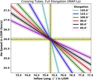
Figure 15. On the IMAP, the IMAP-Lo instrument will follow λPeak with a wide range of different elongations ηE
(shown here from 60° to 135°) to provide ISN parameter tubes that cross over a narrow range of local interstellar longitudes. The yellow cross-hatch shows an uncertainty range of ∼±008 in ecliptic longitude and ∼±0.09 km s−1 in local interstellar inflow speed.
Download figure:
Standard image High-resolution imageWe are deeply indebted to all of the outstanding people who have made the IBEX mission possible, and we are grateful to all of the dedicated people who are working actively to make the IMAP mission a reality. This work was funded by the IBEX mission as a part of the NASA Explorer Program (NNG17FC93C; NNX17AB04G), and by IMAP as part of the Solar Terrestrial Probes Program (NNN06AA01C).
Appendix A: Frame-of-Reference Transforms in the IBEX-Lo Distributions
In treating neutral He populations observed by IBEX-Lo, it is necessary to understand the frame of reference observed. The data are taken in the spacecraft reference frame. There are then two reference frame transformations applied. The first of these shifts from the spacecraft reference frame into the frame moving with Earth about the Sun. The second reference frame shifts into the inertial reference frame moving with the Sun.
In both frame transformations, it is important to understand several underlying geometrical considerations, as outlined here. The velocity of a neutral He atom (mass mHe) in the pristine interstellar medium is denoted v ∞. In its transit to 1 au (denoted r1), the atom falls into Earth's gravitational potential and it increases to speed v1. Conservation of energy dictates that

Taking an initial speed of v∞ = 26 km s−1, we find v1 = 49.5 km s−1 at 1 au. The Earth moves around the Sun at a speed  km s−1, and therefore the particle moves at a speed v1E
≈ v1 + vE
= 79.4 km s−1 in the reference frame of Earth. Note that we have made use of the fact that IBEX observes neutral atoms when they are near the perihelion in their trajectories and where the motion of Earth about the Sun opposes the velocity of the neutral atom. We have also taken the trajectories to move almost within the equatorial plane. As a result the atoms move approximately in the azimuthal direction in the retrograde direction. The speed v1E
has an associated energy of 131 eV.
km s−1, and therefore the particle moves at a speed v1E
≈ v1 + vE
= 79.4 km s−1 in the reference frame of Earth. Note that we have made use of the fact that IBEX observes neutral atoms when they are near the perihelion in their trajectories and where the motion of Earth about the Sun opposes the velocity of the neutral atom. We have also taken the trajectories to move almost within the equatorial plane. As a result the atoms move approximately in the azimuthal direction in the retrograde direction. The speed v1E
has an associated energy of 131 eV.
In the following, we treat the distributions observed in Appendices A.1 and A.2. Specifically, the discussion in Appendix A.1 pertains to the observed angular distribution, and Appendix A.2 pertains to the observed speed distribution. Lastly, we discuss corrections for aberration in Appendix A.3 in the moving spacecraft reference frame.
A.1. Angular Distributions
In this appendix, we treat the angular distribution of neutral atoms observed by IBEX-Lo as the spacecraft spins at its spin axis. In the pristine interstellar medium, the distribution of He atoms is taken as a Maxwell–Boltzmann distribution:
where f∞( v ∞) represents the distribution function of He atoms in the pristine interstellar medium, or more specifically, the number of He atoms per unit volume and per unit velocity space volume centered on velocity v ∞. The bulk velocity of neutral He atoms in the pristine ISM is u He. We consider particles that are relatively close to the peak in the distribution. Lee et al. (2012) provide a description of the geometry of incident He atoms. We take the angle ψ to represent the angle of the hyperbolic atom trajectory relative to the ecliptic plane in the inertial reference frame. Here, the peak of the distribution occurs at an angle ψ = −β ≈ −5°. Because the observations are made close to the peak in the distribution, we take the angle α = ψ + β relative to the peak of the distribution and approximate the speed as ∣v∞∣ ≈ ∣uHe∣. The previous considerations about particle speed apply and the particle speed is v1 = 49.5 km s−1 in the inertial frame. The particle velocity at 1 au in the inertial reference frame is

where  is the direction of Earth's prograde motion and
  is the northerly direction perpendicular to the ecliptic plane.
Because the neutral particle sensor does not discriminate the incoming particles for their energy within an energy step, we treat the incoming particle distribution as an angular distribution with respect to the peak of the distribution. Because the particle passes close to perihelion at 1 au, the plane defined by the Sun–Earth vector and particle velocity vector at 1 au is also the plane in which
v
∞ must lie. As a result, the angle between
v
∞ and
v
He is approximated by angle α. The term ![${[{{\boldsymbol{v}}}_{\infty }-{{\boldsymbol{v}}}_{\mathrm{He}}]}^{2}$](https://content.cld.iop.org/journals/0067-0049/258/1/7/revision2/apjsac2fa9ieqn69.gif) is therefore given by
is therefore given by  . The Maxwell–Boltzmann distribution in the pristine interstellar medium is expressed as follows:
where  . With THe ≈ 7600 K and vHe = 26 km s−1, we find Δα = 875. The FWHM of the angular distribution is

In the frame of reference of Earth, the particle speed is enhanced, as discussed previously. The particle velocity in the Earth frame is  , and the angle ψE
relative to the ecliptic in this frame is
, and the angle ψE
relative to the ecliptic in this frame is
This effect reduces the FWHM of the distribution in the Earth frame to ΔαE−FWHM ≈ 33°. This will also shift the peak of the distribution from an angle of ψ ≈ −5° to ψE
≈ −31.
A.2. Speed Distributions and Rates
In the previous appendix, we discussed the angular distribution of ISN atoms. We did so by leaving the speed constant and varying the angle relative to the inflow peak. In this appendix, we now hold the angle fixed and examine the variation in the distribution function as a function of the speed of incident atoms. At the peak of the distribution, the corresponding velocity of neutral atoms in the pristine interstellar medium is parallel to the bulk flow motion. Therefore, v ∞∥ u He and Equation (A2) becomes
Equation (A1) can be applied directly to eliminate ∣ v ∞∣:
Schwadron et al. (2009b) developed an analytic solution for the survival probability, Sp which can be applied here:
where βp1 is the photoionization rate at 1 au and n1 is the solar wind density at 1 au. The speed  , where u is the solar wind speed, and
  . Here f∞1 represents the distribution function near the peak as a function of particle speed in the inertial frame of the Sun. Because the trajectories are near perihelia, we take v1E
≈ v1 + vE
. Therefore, the distribution function of the particle speed in the Earth frame is
. Here f∞1 represents the distribution function near the peak as a function of particle speed in the inertial frame of the Sun. Because the trajectories are near perihelia, we take v1E
≈ v1 + vE
. Therefore, the distribution function of the particle speed in the Earth frame is
Lastly, we take into account the spacecraft motion about Earth. We continue to use the approximation that atoms move predominantly in the direction parallel with Earth's motion and take into account only the component of spacecraft in this direction, vSC−E. In GSE coordinates, vSC−E = −vSC−y . If the spacecraft moves in the prograde direction, the speed of the atom should be increased, whereas retrograde motion of the spacecraft decreases the speed of the incident atom. As a result the atom's speed in the spacecraft frame is approximated by v1SC ≈ v1E + vSC−E, and the distribution function in terms of this speed is
For each of these distributions, we estimate the count rate near the peak of the distribution. As already discussed, the angular distribution of incident atoms is broad and fills the IBEX-Lo aperture (the solid angle of IBEX-Lo is denoted ΔΩIBEX−Lo). The speed distribution is extremely narrow compared to the response of the instrument in particle speed due to the broad and flat energy response of sputtered ions. Therefore, the distribution is approximated as a delta function, and in the spacecraft reference, the rate is approximated as

We then treat the Gaussian as a function of speed as a delta function,
Therefore, we approximate the integrated rate in the spacecraft reference frame as
The integrated rate in the frame comoving with Earth is approximated as
and the integrated rate in the inertial frame is approximated as
These expressions for the rates are useful in estimating how the rates should be modified to take into account frame transformations. We take the observed rate in the S/C frame as OSC and project these rates into the frame comoving with Earth,  , and into the inertial frame
  :
:
Lastly, we estimate a quantity proportional to the distribution in the inertial frame

A.3. Aberration Corrections
The pointing of the IBEX spin axis is close to but not generally oriented directly at the Sun. It drifts westward of the Sun as IBEX orbits the Sun with Earth, and exact Sun-pointing occurs at a specific ecliptic longitude for each orbit arc. The S/C motion relative to Earth leads to "off-pointing" effects and are corrected for by defining an effective longitude where the spacecraft would be Sun-pointed (i.e., for E
= 0°, where the ecliptic spin-axis angle E
shown in Figure 5 is measured in a right-hand sense from the spin axis to the S/C-to-Sun vector, and the elongation angle measured from the IBEX-Lo boresight to the S/C-to-Sun vector is ηE
= E
+ 90°). More generally, we define the "aberrated longitude," λa
, as the effective longitude where the spacecraft attains a specific ecliptic spin-axis angle, E
, for arbitrary values of E
.
We take the spacecraft to have velocity v SC = v E + v SC−E in the inertial reference frame. Here, v E is Earth's velocity and v SC−E is the velocity of the spacecraft in the Earth reference frame. We take the neutral atom velocity in the inertial frame to be v 1. Therefore, the neutral atom velocity v 1SC in the frame of the spacecraft is

We take the neutral atom velocity to be in the ecliptic plane, and for IBEX-Lo, the boresight is almost exactly normal to the spin axis. Therefore for an instantaneous ecliptic spin-axis angle E0, the neutral atom velocity in the S/C frame is given by

where the x-axis is directed at the Sun, and the y-axis is directed in the retrograde direction. Therefore, the instantaneous ecliptic spin-axis angle is
In order to shift the instantaneous pointing at the S/C longitude λ0 to an aberrated longitude λa
with exact Sun-pointing (E
= 0°), we would need to translate the S/C back in longitude, Δλ = λa
− λ0 = − E0. Conversely, the shift to a specific (positive) ecliptic spin-axis angle E
requires a translation of the S/C forward in longitude,

Note that the trivial case of a translation to E
= E0 results in a null translation, Δλ = 0°, as required. Substitution of Equation (A22) into Equation (A23) results in the following expression for the translation to the aberrated longitude,

This correction is almost exact for E
= 0° and remains a good approximation as long as E ≪ 1 when expressed in radians.
Appendix B: ISN Parameter Tubes
The starting point for the solution of the parameter tube is the relations from Lee et al. (2012). The neutral atom energy, E, angular momentum, ℓ, and the eccentricity, , are given by


Here, the angle ϕ is defined by  , where a position vector in the solar reference frame is
R
and the velocity is
V
. The gravitational constant G is associated with k = GmMs
(1 − μ) where Ms
is the solar mass, m is the particle mass, and μ is the ratio of the outward radial force associated with solar radiation pressure to the solar gravitational force for hydrogen. The angle between a point in the trajectory
R
(t) and the position vector of IBEX is θ. The angle θ∞ corresponds to this angle at R(t → −∞) and the angle −θ0 corresponds to perihelion:
, where a position vector in the solar reference frame is
R
and the velocity is
V
. The gravitational constant G is associated with k = GmMs
(1 − μ) where Ms
is the solar mass, m is the particle mass, and μ is the ratio of the outward radial force associated with solar radiation pressure to the solar gravitational force for hydrogen. The angle between a point in the trajectory
R
(t) and the position vector of IBEX is θ. The angle θ∞ corresponds to this angle at R(t → −∞) and the angle −θ0 corresponds to perihelion:


We begin with the argument of the exponential from Lee et al. (2012), Equation (9):
λ is the heliolongitude of the neutral atom and ψ is the tilt of the plane containing the hyperbolic trajectory relative to the ecliptic (see Figure 2 of Lee et al. 2012). Here, the ISM velocity illustrated in Figure 16 is defined as

where β specifies the latitudinal direction of the ISM flow and the sign convention for β is opposite to that adopted by Lee et al. (2012). If we maximize A with respect to λ, by solving ∂A/∂λ = 0, we find

We also maximize A with respect to ψ, by solving ∂A/∂ψ = 0, and find:

Equation (B35) implies that

Using this expression for  in Equation (B34), we find

Taking the ratio of Equation (B36) to (B37), we find

which yields a second expression for  :
:
Using Equation (B39) and Equation (B36) to eliminate  , we solve for ψ:
We then use this solution for ψ to solve for λ:
The solution for λ also allows the solution of the peak latitude:

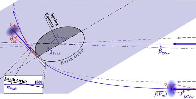
Figure 16. Two ISN flow bulk trajectories with different values for  and
and  (solid and dashed line) are shown along with indications for the ISN velocity distribution at infinity and at 1 au. The ISN flow trajectory plane (gray) intersects Earth's orbit, where IBEX observes the ISN bulk flow at its perihelion or exactly 90° from the Sun (at ecliptic longitude λPeak). The trajectory plane is tilted relative to Earth's orbit by the angle ψPeak, i.e., the latitudinal angle at which the ISN flow arrives at IBEX in the rest frame. The ISN flow longitude
  and latitude
  are also shown.
Download figure:
Standard image High-resolution image
Note that ϕ is in the inertial reference frame. The transformation to the S/C frame is defined as


where the primed variables are in the S/C frame, and VE is Earth's speed in the ecliptic plane. The x, y, and z components of the S/C velocity refer to GSE coordinates with the x direction toward the Sun, the y-direction opposite Earth's motion, and the z-directed north of the ecliptic. Using these relations, we obtain


The quantity  refers to the angle of the incident ENA velocity, not the elongation of the instrument, η, which is related:

Examples of parameter tubes for He are shown in Figure 12 for the following external interstellar parameters: an interstellar flow longitude of λ∞ = 7528, a flow latitude of β = −52 below the ecliptic, and a speed of V∞ = 25.99 km s−1. For a given value of elongation, η, we use the formalism in this appendix to solve for the peak longitude λ0. With this fixed value for the peak longitude, we find how λ∞ varies with V∞, thereby defining a given parameter tube.
Appendix C: Effect of Secondary Populations on the Parameter Tube
One of the issues encountered in the analysis of ISN atoms is the influence of secondary populations. We consider here the influence by treating the deviation from the primary population parameters. At locations far out in the heliosphere, the primary and secondary populations are represented by independent Gaussian distributions. If only the primary population is present, the Gaussian peak is naturally the maximum of the distribution. When we consider the sum of a primary and a secondary population, the maximum of the distribution shifts slightly from the primary peak.
Because the maximum of the sum of Gaussians must fall along the line between the populations, it is convenient to reduce the problem to the deviation from the primary distribution along the line between the two distributions. We take the variable w to represent the speed deviation from the primary distribution with w = 0 corresponding to the peak in the primary distribution. The peak in the secondary population exists at w = ws and the sum of the two distributions takes the form

Here, the subscripts p and s refer to primary and secondary populations, respectively. The B terms are inversely related to temperature, Bp = mHe/(2kTp ) and Bs = mHe/(2kTs ), where Tp and Ts are the primary and secondary temperatures, respectively.
In finding the maximum in the distribution, we set ∂f/∂w = 0. This yields the following equation:
The equation can be rewritten in a slightly more convenient form:

Here  and are used in a Taylor series expansion. Holding on to terms only to first-order yields

The solution for the peak in the distribution is given by
which we rewrite for convenience in the following form,

where
Note that the relative amplitude of the secondary population at the primary peak is ![${g}_{s}=({A}_{s}/{A}_{p})\exp [-{B}_{s}{w}_{s}^{2}]$](https://content.cld.iop.org/journals/0067-0049/258/1/7/revision2/apjsac2fa9ieqn87.gif) , which Kubiak et al. (2016) find to be gs
=0.015. Given a primary temperature of Tp
∼ 7496 and a secondary temperature of Ts
∼ 9500, we find that αs
= 1 + (Ts
/Tp
)/gs
≈ 85.49.
, which Kubiak et al. (2016) find to be gs
=0.015. Given a primary temperature of Tp
∼ 7496 and a secondary temperature of Ts
∼ 9500, we find that αs
= 1 + (Ts
/Tp
)/gs
≈ 85.49.
In practice we need to know the velocity of the inflow (the peak). We calculate this using the vectors u p and u s for the primary and the secondary flows:

As an example, we apply this solution using the primary vector Table 1 with longitude 7528, latitude −52 and speed = 25.99 km s−1. For the secondary population, we use results from Kubiak et al. (2016) with longitude 7157, latitude −1195, and speed 11.28 km s−1. The combined distribution yields a peak with longitude 7526, latitude −523, and speed 25.82 km s−1.