The Cosmic Ultraviolet Baryon Survey (CUBS). VIII. Group Environment of the Most Luminous Quasars at z ≈ 1

The MUSE galaxy survey is the deepest and most compact component of our ground-based optical spectroscopic observations, aiming to target galaxies as faint as 0.01 L_* at z = 1 within ≲30'' from the central quasar. The MUSE survey is carried out on the VLT UT4 in service mode under program ID 0104.A-0147 (PI: Chen). The observations cover $1^{\prime} \times \,1^{\prime}$ FOVs with plate scales of 02 and spectral resolution of ≈120 km s⁻¹ at 7000 Å. The observations are in the wide-field mode (WFM) with ground layer adaptive optics (AO) assistance to ensure uniform image quality of <08 across all fields. The limiting magnitude (3σ) of the detected sources in the MUSE data cubes are AB(r) ≈ 26 in the pseudo-r band (Qu et al. 2023), sufficient to identify faint galaxies down to M_⋆ ≈ 10⁸–10⁹ M_⊙. The MUSE data cubes are reduced using the standard ESO MUSE pipeline (Weilbacher et al. 2020) and the custom data reduction package CUBEXTRACTOR (Cantalupo et al. 2019). Additional details of the MUSE observations are described in Chen et al. (2020).

Deep H-band images were obtained in 2017 October using the FourStar Infrared Camera (Persson et al. 2013) on the Magellan Telescopes. The data reduction was performed using the FourCLift custom package (details described in Kelson et al. 2014) and following the procedures in Kelson et al. (2014) and Rudie et al. (2017). The exposure in each field is roughly 2000–3000 s, and the limiting magnitude (3σ) of the detected sources is ≈24.5 mag (Qu et al. 2023). The median seeing of the final images is ≈05.

While using the MUSE WFM AO observation setup ensures a uniform imaging resolution, the use of wavefront lasers produces a gap at 5800–5965 Å in the spectra. We obtained supplementary spectra from the Magellan Echellette (MagE) Spectrograph for quasars with the Mg ii line in/near the sodium gap (J0333, J2135, J2245, J2308) to ensure good spectral coverage around the broad Mg ii line for BH mass estimation. The observations were carried out on 2021 September 29 and 30 on the Magellan Baade Telescope. Two to three exposures of 300–600 s, depending on the quasar luminosity, were taken for each source to mitigate cosmic rays. The final reduced spectral range is 4000–9900 Å with median spectral resolution of ≈1 Å and spectral sensitivity (1σ) of 1–4 × 10⁻¹⁷ erg cm⁻² s⁻¹ Å⁻¹. We follow the standard data reduction pipeline with CarPy (Kelson et al. 2000; Kelson 2003) to reduce the data and match the flux scale to the MUSE spectra.

We identify all continuum sources in the MUSE white-light image with Source Extractor (Bertin & Arnouts 1996) for redshift measurements. For the quasars, we extract the optical spectra within apertures that include >95% of the quasar light and measure the redshifts based on narrow [O ii] emission lines, which results in a typical redshift uncertainty of 20–30 km s⁻¹ (Hewett & Wild 2010). For galaxies, the spectra of each source are extracted within a ≈06 radius using the Python MUSE data analysis package mpdaf (Bacon et al. 2016). We then follow the procedures described in Johnson et al. (2018) and Helton et al. (2021) to determine the redshift of each source. To briefly summarize, each spectrum is fitted with a linear combination of Sloan Digital Sky Survey (SDSS) galaxy eigenspectra over a wide redshift grid, and the best-fit redshift is identified at the global minimum in the resulting χ² grid. We then visually inspect the best-fit spectra to assign a quality ranking for each redshift. We define the robust double-feature redshifts to have good fits around at least two spectral features (including both emission and absorption, visually evaluated by trained team members) and the single-feature redshift to have good fits around one spectral feature, and the rest of the redshifts are discarded. It is possible that the single-feature redshifts are not unique solutions, in these cases, we only include them in the final redshift measurement after all other possible solutions (e.g., a different emission line is well-fitted to the spectral feature) are ruled out.

Figure 1 shows the redshift distribution. Across all 15 quasar fields, we identified 1542 continuum sources (excluding stars) and measured 712 double-feature redshifts and 109 single-feature redshifts. The redshift success rates are approximately 40%–65% across all fields. The primary reason for not measuring a redshift is usually because of low signal-to-noise ratios in the spectra or the lack of spectral features. Our MUSE redshift survey is most sensitive to redshifts z < 1.5, where strong line features (e.g., Hα, Hβ, O iii, [O ii] lines, and stellar absorption features) are within the MUSE spectral coverage.

Zoom In Zoom Out Reset image size

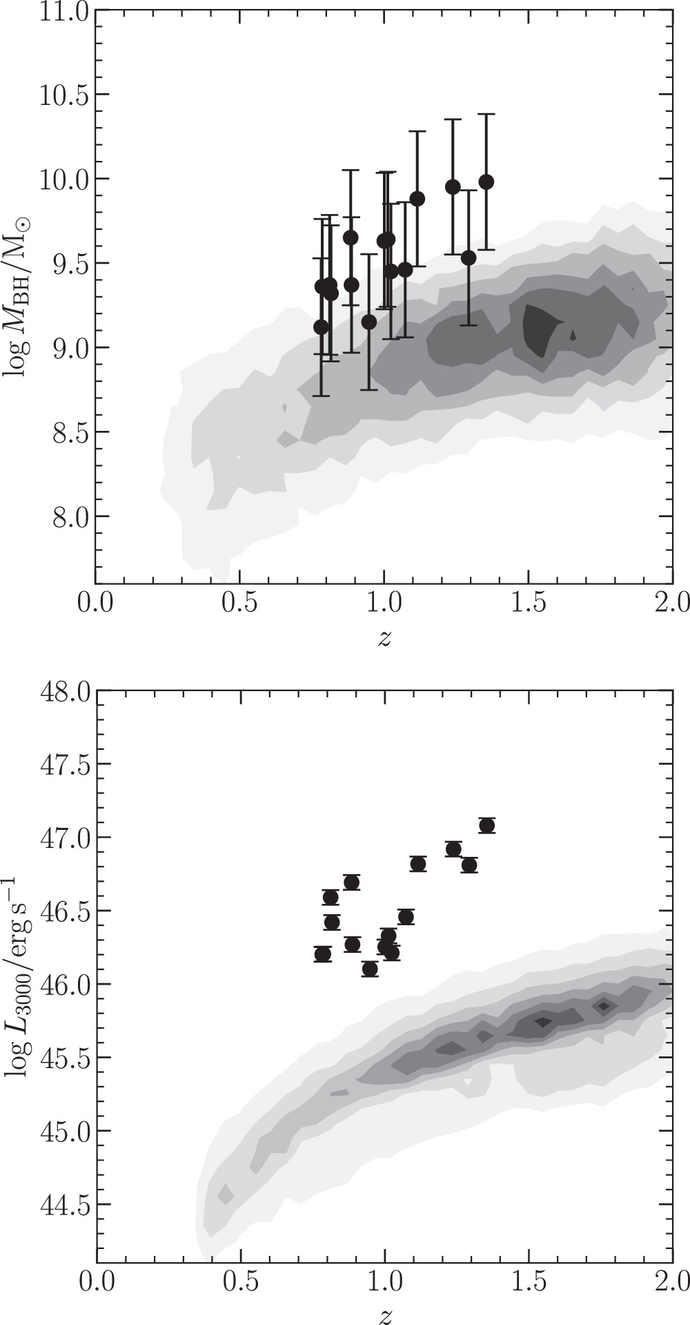
BH masses are estimated through the single-epoch method (Shen et al. 2011). Assuming the broad-line region (BLR) is virialized, we can measure the BH mass from a single spectrum by estimating the BLR size from the quasar luminosity with the radius–luminosity relation (Bentz et al. 2013) and the BLR virial velocity from the width of a broad emission line (e.g., the 2800 Å Mg ii line). We extract quasar spectra from apertures of 10 pixels centered on the quasar positions in the MUSE data cube, which roughly encompass 95% of the total light. For the quasars where the Mg ii line falls into the sodium gap, we use the supplementary quasar spectra from the MagE observations. We fit the quasar spectra with a power-law continuum, the Fe ii pseudo-continuum, and a series of Gaussian profiles for each broad line using the code PyQSOFit (Guo et al. 2018). The host galaxy light is expected to be very faint compared to the bright core for these quasars, so we do not perform host decomposition in PyQSOFit. We include up to three broad components, one narrow component, and an additional wing component to model the Mg ii line. Finally, we follow the recipe from Shen et al. (2011) to estimate BH masses using the luminosity at 3000 Å and the combined full width at half-maximum from the Mg ii line for each quasar. The BH mass uncertainties from the single-epoch BH mass estimator with the Mg ii line is roughly 0.4 dex (Shen et al. 2023), though it might be larger for the CUBS quasars since they are outliers in luminosity compared to the quasar population used in reverberation mapping studies. The virial BH masses and the luminosity at 3000 Å (as functions of redshift) are plotted in Figure 2 and tabulated in Table 1.

Zoom In Zoom Out Reset image size

Table 1. Summary of the Quasar Properties

Quasar Name	Other Name	R.A.	Decl.	z	$\mathrm{log}{M}_{\mathrm{BH}}/{M}_{\odot }$	$\mathrm{log}{L}_{3000}/$ erg s−1	R
		(J2000)	(J2000)
J0028-3305	...	00:28:30.41	−33:05:49.25	0.8873	9.37	46.3	<11
J0110-1648	...	01:10:35.51	−16:48:27.70	0.7823	9.12	46.2	230
J0111-0316	...	01:11:39.17	−03:16:10.89	1.2384	9.95	46.9	<6
J0114-4129	HE 0112-4145	01:14:22.12	−41:29:47.29	1.0238	9.45	46.2	18
J0119-2010	...	01:19:56.09	−20:10:22.73	0.8163	9.32	46.4	<7
J0154-0712	...	01:54:54.68	−07:12:22.17	1.2930	9.53	46.8	<8
J0248−4048	HE 0246-4101	02:48:06.29	−40:48:33.66	0.8844	9.65	46.7	4
J0333-4102	HE0331-4112	03:33:07.08	−41:02:01.15	1.1153	9.88	46.8	<6
J0357-4812	PKS 0355-483	03:57:21.92	−48:12:15.16	1.0128	9.64	46.3	783
J0420-5650	HE 0419-5657	04:20:53.91	−56:50:43.96	0.9481	9.15	46.1	<18
J0454-6116	...	04:54:15.95	−61:16:26.56	0.7861	9.36	46.2	7
J2135-5316	...	21:35:53.20	−53:16:55.82	0.8115	9.37	46.6	<4
J2245-4931	PKS 2242-498	22:45:00.21	−49:31:48.46	1.0011	9.63	46.3	2779
J2308-5258	HE 2305-5315	23:08:37.80	−52:58:48.94	1.0733	9.46	46.5	<10
J2339-5523	HE 2336-5540	23:39:13.22	−55:23:50.84	1.3544	9.98	47.1	339

Note. The table columns are quasar name, alternative quasar names in the literature, quasar R.A., decl., redshift, BH mass, luminosity at 3000 Å, and radio-loudness (R).

Download table as:  ASCIITypeset image

We obtain the radio properties of the quasars by crossmatching with the Rapid Australian Square Kilometre Array Pathfinder (ASKAP) Continuum Survey (RACS) DR1 catalog (Hale et al. 2021). ASKAP surveys the sky south of +41° decl. at a central frequency of 887.5 MHz with a spatial resolution of ∼15'' (convolved to 25'' for the source catalog). We first match the quasar positions in the RACS DR1 catalog for all sources within 30''. A total of seven quasars have radio counterparts; two (J0110, J2245) show extended/lobed detection (lobe-dominated), and the rest (J0114, J0248, J0357, J0454, J2339) show unresolved single detection (core-dominated or unresolved). For the lobed-dominated sources, we use the total source flux as the radio flux. We calculate the radio-loudness (R) as the ratio of the flux density at 6 cm and 2500 Å in the rest frame, R = f_ν,6cm/f_{ν,2500 Å} (Stocke et al. 1992). The UV flux density f_{ν,2500 Å} is calculated from the best-fit quasar spectra from PyQSOFit. The rest-frame 6 cm flux density is extrapolated from the RACS radio flux by assuming a spectral index α (F_ν ∝ ν^α ) of −0.5. The RACS DR1 catalog requires a 5σ detection for sources to be included in the catalog and has an overall 95% point source completeness at an integrated flux density ≈3 mJy. Adopting 3 mJy as the upper limit in radio flux density, we find most of the non-detected sources have an upper limit of R ≲ 10. Typically, quasars with R ≳ 10 are defined as radio-loud quasars (Kellermann et al. 1989). We identify five radio-loud quasars, and the remaining quasars are undetected or radio-quiet. For the quasars above decl. of −40°, we also cross check with the FIRST and VLASS surveys and find consistent radio properties at 3 cm. The radio-loudness parameter R is tabulated in Table 1.

To identify member galaxies in the quasar galaxy groups, we search for galaxies close to the quasar redshift in the MUSE field of view. We calculate the group mean velocity (μ_Vel) and velocity dispersion (σ_Vel) by fitting the galaxy relative velocity within ∣ΔV∣ < 1500 km s⁻¹ of the quasar redshift with a normal distribution. The initial velocity range (∣ΔV∣ < 1500 km s⁻¹) roughly equals the velocity dispersion of the most massive galaxy clusters. For more robust identification, we recalculate the new μ_Vel and σ_Vel after sigma-clipping at 3σ and remove all sources beyond 3σ of the original μ_Vel and σ_Vel, this calculation is repeated two to three times until the group member identification has converged. Figure 3 shows the MUSE white-light images and the galaxies identified within each quasar group. Figure 4 shows the velocity distribution of each group. All galaxies within ∣ΔV∣ < 3000 km s⁻¹ of the quasar are shown in open histograms, and the identified group members are shown in orange (double-feature redshifts) and gray (single-feature redshifts) histograms.

Zoom In Zoom Out Reset image size

Zoom In Zoom Out Reset image size

The groups include 3–23 galaxies around the quasars (including the quasar host galaxy), indicating the CUBS quasars reside in poor to massive groups. For groups with N_gal > 5, we report the final μ_Vel and σ_Vel of the group. The velocity dispersion ranges from 150–600 km s⁻¹ (except for J2339), which suggests our initial velocity search range is sufficient. While there could still be chance projections in the identified group members, the majority of the galaxies in N_gal > 5 groups are projected within the virial radii, estimated with the derived halo masses (see Section 5.1). In addition, most of the identified group members are likely bound in N_gal > 5 groups, their relative velocities to the quasars are less than the escape velocities at the corresponding galaxy distances. Removing the few galaxies near the virial radius or above the escape velocity does not change the estimated velocity dispersion or halo mass significantly. The final group size, mean velocity, and velocity dispersion are tabulated in Table 2.

Table 2. Summary of the Galaxy Groups (within the MUSE FOV)

Quasar Name	Ngroup	δg	σδ	μVel	σVel	σVel,corr	$\mathrm{log}{M}_{200}/{M}_{\odot }$
				(km s−1)	(km s−1)	(km s−1)
J0028-3305	7	${10.1}_{-3.7}^{+4.8}$	2.73	526	270	280	13.2
J0110-1648	3	${3.7}_{-2.3}^{+3.3}$	1.65	⋯	⋯	⋯	⋯
J0111-0316	3	${3.7}_{-2.3}^{+3.3}$	1.65	⋯	⋯	⋯	⋯
J0114-4129	9	${13.2}_{-4.2}^{+5.3}$	3.12	20	400	410	13.6
J0119-2010	8	${11.6}_{-4.0}^{+5.0}$	2.93	437	460	480	13.9
J0154-0712	7	${10.1}_{-3.7}^{+4.8}$	2.73	189	420	440	13.7
J0248-4048	6	${8.5}_{-3.4}^{+4.5}$	2.50	−38	110	110	12.1
J0333-4102	8	${11.6}_{-4.0}^{+5.0}$	2.93	−468	300	310	13.3
J0357-4812	23	${35.3}_{-7.0}^{+8.1}$	5.01	402	570	580	14.1
J0420-5650	4	${5.3}_{-2.7}^{+3.8}$	1.98	⋯	⋯	⋯	⋯
J0454-6116	19	${29.0}_{-6.4}^{+7.4}$	4.56	157	290	300	13.3
J2135-5316	3	${3.7}_{-2.3}^{+3.3}$	1.65	⋯	⋯	⋯	⋯
J2245-4931	9	${13.2}_{-4.2}^{+5.3}$	3.12	143	240	250	13.1
J2308-5258	5	${6.9}_{-3.1}^{+4.1}$	2.26	⋯	⋯	⋯	⋯
J2339-5523	13	${19.5}_{-5.2}^{+6.2}$	3.77	−216	940	960	14.6
J2339-5523 a	7	${10.1}_{-3.7}^{+4.8}$	2.73	592	370	390	13.5

Note. The table columns are quasar name, number of group galaxy members (including the quasar host galaxy), overdensity, significance of overdensity (σ_δ = δ_g/Δδ_g ), mean velocity of the galaxy group with respect to the quasar, velocity dispersion of the galaxy group, the corrected velocity dispersion (see Section 5), and the estimated halo mass.

^a The group measurements of J2339 when assuming a bimodal velocity distribution, the group with mean velocity closer to the quasar velocity is reported here.

Download table as:  ASCIITypeset image

The velocities of galaxies in the field of J2339 show a bimodal distribution, suggesting there might be two individual galaxy groups perhaps starting or undergoing a merger event. When fitted with two normal distributions, we find two distinct groups of 7 (closer to the quasar redshift) and 6 galaxies with similar velocity dispersion of ≈350 km s⁻¹. While ∼1000 km s⁻¹ (σ_Vel of J2339 fitted with a single Gaussian) is still within a reasonable range for a galaxy group/cluster, ≈300 km s⁻¹ is more consistent with other groups and better describes the bimodal velocity distribution. We report the group properties of the group closer to the quasar redshift in Table 2 and plot both velocities in the remaining figures of this paper.

To study the quasar environments, we search for overdensities around the central quasars using the relative velocity distribution. Following Stott et al. (2020), we calculate the overdensity δ_g using the equation

$$\begin{eqnarray}&&{\delta }_{g}=\displaystyle \frac{{N}_{\mathrm{group}}-{N}_{\mathrm{bkg}}}{{N}_{\mathrm{bkg}}},\end{eqnarray} \tag{ 1 }$$

where N_group is the number of objects in each quasar group and N_bkg is the expected number of background objects without the presence of any structure. We calculate N_bkg by stacking the relative velocity distribution for all quasar fields with a bin size of 3000 km s⁻¹ (i.e., ±1500 km s⁻¹), centered on the quasar systematic velocity. The velocity bin size is chosen to ensure all identified group galaxies are within the center bin of the stacked histogram (see Figure 4). The full ΔV range of ±36,000 km s⁻¹ shown in Figure 5 roughly corresponds to 0.2–0.3 in Δz depending on the quasar redshift.

Zoom In Zoom Out Reset image size

Figure 5 shows the stacked distribution of relative velocity from the central quasars. The median (16th and 84th percentiles) number counts of the background galaxies are N_bkg = 9.5 (6.0, 14.3) when excluding the central bin. The stacked δ_g across all 15 quasar fields is ${12.4}_{-1.1}^{+1.2}$ (i.e., ≈11σ), and the individual δ_g of each quasar field ranges ≈4–35 (tabulated in Table 2) using the galaxy counts in each field and the average background galaxy count across 15 fields, N_bkg = 0.63. The uncertainties of δ_g are calculated through the Bayesian approach described in Kraft et al. (1991) for determining the Poisson confidence level for a number count given by a background. Following the convention in the literature, we find 11 quasars reside in >2σ overdense environments (i.e., galaxy groups with ≳ 5 members), and 5 quasars reside in >3σ overdensity (≳ 9 members). When excluding the single-feature redshifts, the results remain unchanged; the stacked δ_g is ${14.9}_{-1.3}^{+1.4}$ (i.e., ≈11σ), and the same 11(5) quasars are above the >2σ(3σ) threshold. While N_bkg and δ_g depend on the exact choice of the velocity grid, the significance of overdensity (σ_δ ) remains consistent with bin sizes of 2500–4500 km s⁻¹. We note that the decline at ΔV > 25,000 km s⁻¹ in the stacked relative velocity (Figure 5) could be due to the lower completeness in redshift measurement at z > 1. However, the overdensity measurements are not sensitive to the exact choice of the full ΔV range, provided that it is large enough for accurately estimating the background galaxy counts. For our sample, the median background galaxy count remains consistent at N_bkg = 9 − 10 with full ΔV ranges of ±24,000–36,000 km s⁻¹.

The MUSE FOV (1$^{\prime} \approx 500$ kpc at z ≈ 1) might not be large enough to survey all galaxies in the galaxy groups/clusters. We find 1–3 additional galaxy group members within a projected distance of 500 kpc around half of the CUBS quasars in the LDSS3/IMACS redshift surveys. These additional galaxies are all found in the fields of the >2σ overdense quasars and the measured velocity dispersion is consistent within 10% if these galaxies are included. The only two exceptions are the fields J0114 and J0119. The additional galaxy found in the J0114 field lies at the edge of the velocity distribution and thus increased the velocity dispersion by ≈30% when included. For the field of J0119, six additional galaxies were found in the LDSS3 FOV near the quasar redshift, which made J0119 one of the most overdense groups in the sample. The estimated velocity dispersion of the galaxy group around J0119 decreases by ≈20% when including the six additional galaxies. However, the source selection of the LDSS3/IMACS redshift surveys is based on color selection to prioritize galaxies in the quasar foreground and the redshift surveys are much shallower than the MUSE observation. Therefore, it is nontrivial to quantify the selection effect in overdensity estimation, and we choose to focus on the overdensity in the MUSE FOV only.

We estimate the stellar masses for the galaxies within the CUBS quasar groups by galaxy spectral modeling with the code BAGPIPES (Carnall et al. 2018, 2019) using both spectroscopic and photometric observations. We extract the galaxy spectra within a ≈06 radius using mpdaf, i.e., the same spectra as used for the redshift measurements. We extract deep psuedo-photometry in the g, r, and i bands by convolving the MUSE data cubes with the g, r, i psuedo-bandpasses (i.e., boxcar functions around 4800–5800, 6000–7500, and 7500–9000 Å, following previous CUBS papers). For bright galaxies (i ≳ 20.5 mag), we supplement with the g-, r-, i-, z-, Y-band photometry from the Dark Energy Survey Y3 GOLD catalog (Sevilla-Noarbe et al. 2021). Finally, we include the H-band photometry from our FourStar observations. For the MUSE and H-band photometry, we first perform Source Extractor on the pseudo-r band image and use the pseudo-r band segmentation map to extract photometry from each MUSE and H-band image to ensure the photometry is obtained from the same region. The photometric uncertainties are set to be 10%.

BAGPIPES is a Bayesian fitting code that can model galaxy spectra with spectroscopic and photometric data simultaneously. We model the galaxy spectra with the Kroupa (2001) initial mass function, Bruzual & Charlot (2003) stellar population models, an exponential star formation history, and include nebular emission and dust extinction models from Calzetti et al. (2000). To fit spectroscopic and photometric data simultaneously, we allow zeroth to second order calibrations and a noise scaling parameter that accounts for relative flux calibration as suggested by Bagpipes, e.g., corrections for aperture or template mismatch, underestimation of uncertainties, and wavelength-dependent flux calibration in the spectroscopic data. As a robust check, we tested different star formation histories (exponential and double power law) and dust extinction models (Calzetti et al. 2000 and Charlot & Fall 2000) and found the estimated galaxy masses to be consistent regardless of the model and parameter setup.

Galaxies closest to the central quasar are often heavily contaminated, or even outshined, by the quasar light. For galaxies very close to the quasars, we perform quasar light subtraction using the methods from Johnson et al. (2018) and Helton et al. (2021) to recover the quasar-subtracted spectra and photometry for the galaxies closest to the quasars. In short, we model the light around the quasars using a linear combination of galaxy and quasar eigenspectra to decompose the quasar and galaxy light. For the H-band image, we use GALFIT (Peng et al. 2002) to perform 2D surface brightness decomposition to remove the central quasar light. Finally, we follow the same procedures described previously to extract MUSE spectra, pseudo-photometry, and H-band photometry from the quasar-subtracted data cubes and images. Of the 11 galaxies that are strongly contaminated by the quasar light, we were able to recover the galaxy photometry and stellar mass for four galaxies.

The derived properties of the galaxies in each quasar group are tabulated in Table 3, along with their relative velocities and projected distances from the central quasar. The estimated galaxy masses are $8.5\lt \mathrm{log}({M}_{\star }/{M}_{\odot })\lt 11.6$, with median $\mathrm{log}({M}_{\star }/{M}_{\odot })=9.9$, and the typical mass uncertainty from Bagpipes is ≈0.1 dex, excluding systematic uncertainties.

Table 3. Summary of the Galaxy Properties in Each Quasar Field

Quasar Name/	R.A.	Decl.	z	mr	MB	B − I	$\mathrm{log}{M}_{* }/{M}_{\odot }$	Δ v	Δ θ	Δ d
Galaxy ID	(J2000)	(J2000)		(AB)	(AB)	(AB)		(km s−1)	(arcsec)	(kpc)
J0028
1	00:28:30.89	−33:05:55.89	0.8920	23.0	−18.6	1.8	${10.05}_{+0.16}^{-0.16}$	+747	9.8	76
2	00:28:29.51	−33:05:52.16	0.8898	23.9	−17.9	1.8	${9.45}_{+0.05}^{-0.05}$	+397	13.7	106
3	00:28:31.20	−33:06:14.13	0.8916	23.1	−18.1	0.7	${8.86}_{+0.18}^{-0.32}$	+683	27.6	214
4	00:28:29.45	−33:06:17.18	0.8929	22.9	−19.0	1.6	${10.05}_{+0.07}^{-0.07}$	+890	31.4	244
5	00:28:30.01	−33:06:20.44	0.8898	20.9	−21.2	1.8	${10.97}_{+0.04}^{-0.06}$	+397	31.8	246
6	00:28:28.14	−33:05:38.58	0.8909	23.9	−17.3	0.9	${9.51}_{+0.20}^{-0.16}$	+572	35.6	276
J0110
1	01:10:35.52	−16:48:13.60	0.7840	23.3	−17.5	1.5	${8.55}_{+0.16}^{-0.15}$	+286	14.1	105
2	01:10:35.73	−16:48:54.70	0.7839	23.9	−17.3	2.2	${9.40}_{+0.20}^{-0.15}$	+269	27.2	203
J0111
1	01:11:39.46	−03:15:39.54	1.2396	22.5	−19.7	0.6	${9.51}_{+0.09}^{-0.09}$	+161	31.6	264
2	01:11:39.65	−03:15:36.30	1.2389	22.6	−21.0	1.6	${10.63}_{+0.06}^{-0.05}$	+60	35.3	294
J0114
1	01:14:22.19	−41:29:51.07	1.0236	23.3	−19.5	2.0	${10.58}_{+0.09}^{-0.09}$	−30	3.9	31
2	01:14:21.42	−41:29:41.37	1.0274	23.4	−19.2	1.6	${9.98}_{+0.06}^{-0.06}$	+533	12.1	97
3	01:14:20.81	−41:29:38.42	1.0241	24.3	−18.0	1.8	${9.61}_{+0.29}^{-0.28}$	+44	21.5	174
4	01:14:20.57	−41:29:44.50	1.0228	21.4	−21.1	1.9	${11.02}_{+0.04}^{-0.03}$	−148	23.4	188
5	01:14:20.12	−41:29:45.25	1.0187	21.5	−21.1	2.2	${11.05}_{+0.06}^{-0.06}$	−755	30.2	243
6	01:14:20.04	−41:29:46.24	1.0243	23.1	−19.5	2.6	${10.76}_{+0.05}^{-0.06}$	+74	31.3	252
7	01:14:20.93	−41:29:14.05	1.0285	22.1	−19.6	0.8	${9.67}_{+0.11}^{-0.10}$	+696	37.7	304
8	01:14:19.70	−41:29:57.59	1.0222	23.5	−18.1	0.4	${9.05}_{+0.18}^{-0.22}$	−237	37.8	304
J0119
1	01:19:56.62	−20:10:22.46	0.8148	20.8	−19.4	0.8	${9.54}_{+0.07}^{-0.08}$	−248	8.0	60
2	01:19:57.44	−20:10:29.75	0.8210	22.3	−18.6	1.0	${9.38}_{+0.10}^{-0.11}$	+776	21.4	162
3	01:19:56.20	−20:10:46.06	0.8175	24.5	−16.3	1.0	${8.39}_{+0.24}^{-0.23}$	+198	23.4	177
4	01:19:54.43	−20:10:34.28	0.8166	21.4	−19.6	1.2	${9.79}_{+0.07}^{-0.05}$	+50	27.5	208
5	01:19:57.90	−20:10:00.94	0.8227	22.8	−18.2	1.3	${9.27}_{+0.05}^{-0.05}$	+1056	34.8	263
6	01:19:57.58	−20:10:55.46	0.8223	21.9	−19.2	1.3	${9.84}_{+0.09}^{-0.07}$	+990	39.6	299
7	01:19:53.71	−20:09:57.14	0.8204	20.3	−20.7	0.5	${9.96}_{+0.06}^{-0.07}$	+677	44.0	332
J0154
1	01:54:54.63	−07:11:55.52	1.2966	23.7	−19.3	1.2	${10.49}_{+0.23}^{-0.26}$	+471	26.7	223
2	01:54:52.99	−07:12:13.70	1.2873	21.8	−21.1	1.4	${10.45}_{+0.06}^{-0.05}$	−745	26.7	224
3	01:54:53.60	−07:11:55.28	1.2968	24.4	−19.4	2.7	${10.24}_{+0.32}^{-0.30}$	+497	31.4	263
4	01:54:55.86	−07:12:49.74	1.2953	23.4	−20.3	2.0	${10.69}_{+0.05}^{-0.06}$	+301	32.8	274
5	01:54:56.13	−07:12:50.45	1.2973	24.1	−18.2	0.8	${8.50}_{+0.36}^{-0.30}$	+562	35.6	298
6	01:54:52.26	−07:12:38.91	1.2948	23.6	−19.5	1.8	${10.31}_{+0.23}^{-0.27}$	+235	40.0	335
J0248
1	02:48:06.70	−40:48:33.82	0.8845	20.7	−20.9	0.8	${10.10}_{+0.01}^{-0.02}$	+16	6.2	48
2	02:48:06.87	−40:48:31.44	0.8834	24.4	−17.3	2.6	${10.01}_{+0.20}^{-0.20}$	−159	9.0	70
3	02:48:07.27	−40:48:14.64	0.8835	24.1	−17.5	1.7	${9.70}_{+0.15}^{-0.15}$	−151	24.1	187
4	02:48:03.85	−40:48:13.47	0.8853	20.7	−21.0	1.8	${10.85}_{+0.04}^{-0.06}$	+143	41.8	324
5	02:48:04.07	−40:48:01.62	0.8839	22.2	−19.5	1.8	${10.14}_{+0.06}^{-0.05}$	−80	46.2	358
J0333
1	03:33:07.34	−41:02:00.99	1.1079	⋯	⋯	⋯	⋯ a	−1049	3.9	32
2	03:33:07.36	−41:01:59.39	1.1114	⋯	⋯	⋯	⋯ a	−553	4.7	38
3	03:33:05.93	−41:01:57.61	1.1104	24.1	−18.9	2.3	${10.27}_{+0.18}^{-0.20}$	−694	17.5	143
4	03:33:06.64	−41:01:44.42	1.1126	23.2	−19.0	0.9	${9.00}_{+0.23}^{-0.23}$	−383	17.9	147
5	03:33:05.72	−41:02:11.20	1.1139	21.9	−20.2	1.3	${9.86}_{+0.19}^{-0.17}$	−198	22.7	186
6	03:33:08.77	−41:01:58.96	1.1121	23.4	−18.9	1.3	${9.40}_{+0.23}^{-0.19}$	−454	25.5	209
7	03:33:10.16	−41:01:51.01	1.1124	21.0	−20.9	0.9	${9.89}_{+0.11}^{-0.11}$	−411	47.3	388
J0357
1	03:57:22.14	−48:12:16.18	1.0176	⋯	⋯	⋯	⋯ a	+715	3.6	29
2	03:57:21.72	−48:12:12.58	1.0148	⋯	⋯	⋯	⋯ a	+298	3.9	31
3	03:57:22.23	−48:12:17.79	1.0132	22.8	−19.9	1.8	${10.65}_{+0.02}^{-0.01}$	+67	5.3	43
4	03:57:21.84	−48:12:26.52	1.0167	23.7	−18.2	0.8	${9.32}_{+0.17}^{-0.20}$	+581	11.4	92
5	03:57:21.15	−48:12:05.54	1.0132	21.7	−20.5	1.7	${10.48}_{+0.05}^{-0.04}$	+67	15.0	121
6	03:57:22.88	−48:12:22.55	1.0147	23.6	−18.8	1.4	${9.47}_{+0.05}^{-0.05}$	+283	16.2	130
7	03:57:21.07	−48:12:04.39	1.0156	23.1	−19.4	1.1	${9.68}_{+0.12}^{-0.11}$	+417	16.7	134
8	03:57:20.85	−48:12:23.18	1.0227	23.2	−19.0	1.7	${9.55}_{+0.24}^{-0.19}$	+1475	17.9	144
9	03:57:20.92	−48:12:01.91	1.0156	22.4	−19.8	1.8	${10.42}_{+0.05}^{-0.06}$	+417	20.0	160
10	03:57:21.93	−48:12:35.99	1.0241	22.5	−19.6	1.2	${9.81}_{+0.15}^{-0.19}$	+1683	20.8	167
11	03:57:22.77	−48:11:58.69	1.0183	22.3	−19.6	0.7	${9.44}_{+0.07}^{-0.06}$	+819	20.9	168
12	03:57:21.91	−48:12:37.02	1.0226	21.6	−20.8	2.6	${11.55}_{+0.15}^{-0.14}$	+1460	21.9	176
13	03:57:23.45	−48:12:17.37	1.0113	22.9	−19.0	1.2	${9.51}_{+0.16}^{-0.14}$	−223	23.1	186
14	03:57:23.47	−48:12:23.92	1.0186	21.9	−20.3	1.6	${10.38}_{+0.05}^{-0.06}$	+864	24.9	200
15	03:57:20.32	−48:12:28.95	1.0168	21.4	−21.1	1.3	${10.44}_{+0.05}^{-0.06}$	+596	27.6	222
16	03:57:23.43	−48:12:32.35	1.0118	21.9	−20.3	2.2	${10.69}_{+0.07}^{-0.03}$	−149	28.5	229
17	03:57:23.25	−48:12:41.09	1.0097	22.8	−18.6	0.4	${9.30}_{+0.09}^{-0.13}$	−462	32.8	263
18	03:57:24.08	−48:12:25.86	1.0171	22.3	−19.8	1.5	${10.14}_{+0.05}^{-0.05}$	+633	34.2	274
19	03:57:20.17	−48:11:48.50	1.0143	23.0	−18.8	0.9	${9.30}_{+0.21}^{-0.17}$	+223	37.4	300
20	03:57:25.00	−48:12:21.41	1.0109	22.0	−19.8	0.5	${9.43}_{+0.06}^{-0.06}$	−283	46.7	375
21	03:57:24.53	−48:12:43.97	1.0135	21.5	−20.7	1.0	${10.14}_{+0.06}^{-0.06}$	+104	48.7	391
22	03:57:25.30	−48:12:44.09	1.0106	22.3	−19.8	1.4	${9.90}_{+0.15}^{-0.14}$	−328	58.4	469
J0420
1	04:20:53.71	−56:50:42.45	0.9476	⋯	⋯	⋯	⋯ a	−77	3.3	26
2	04:20:52.52	−56:50:47.40	0.9465	22.0	−19.3	1.5	${9.67}_{+0.15}^{-0.10}$	−246	21.1	166
3	04:20:54.79	−56:51:01.53	0.9495	23.3	−18.0	0.7	${8.50}_{+0.16}^{-0.16}$	+215	22.0	174
J0454
1	04:54:16.24	−61:16:28.79	0.7879	⋯	⋯	⋯	⋯ a	+302	4.8	36
2	04:54:15.89	−61:16:32.48	0.7867	22.6	−18.4	1.4	${9.48}_{+0.14}^{-0.14}$	+101	6.0	45
3	04:54:15.05	−61:16:36.04	0.7890	21.9	−19.1	1.6	${9.89}_{+0.07}^{-0.07}$	+487	16.6	124
4	04:54:15.10	−61:16:14.03	0.7878	19.0	−22.4	1.3	${11.06}_{+0.04}^{-0.04}$	+285	17.9	134
5	04:54:14.77	−61:16:19.83	0.7853	21.0	−19.9	1.5	${10.13}_{+0.06}^{-0.04}$	−134	19.0	142
6	04:54:16.53	−61:16:09.50	0.7890	20.4	−20.9	1.8	${10.82}_{+0.04}^{-0.03}$	+487	19.1	143
7	04:54:15.85	−61:16:46.43	0.7880	22.8	−17.7	2.2	${9.61}_{+0.25}^{-0.23}$	+319	19.9	149
8	04:54:17.45	−61:16:32.66	0.7869	20.2	−21.2	1.6	${10.92}_{+0.03}^{-0.04}$	+134	23.2	173
9	04:54:17.12	−61:16:42.52	0.7858	22.6	−18.4	1.5	${9.57}_{+0.07}^{-0.06}$	−50	23.7	177
10	04:54:16.98	−61:16:52.17	0.7868	23.0	−18.1	1.0	${9.02}_{+0.08}^{-0.09}$	+117	29.9	223
11	04:54:16.77	−61:15:57.71	0.7867	22.1	−19.2	1.8	${10.07}_{+0.07}^{-0.06}$	+101	31.4	234
12	04:54:18.43	−61:16:37.22	0.7845	23.1	−17.5	0.7	${8.39}_{+0.13}^{-0.12}$	−269	38.7	289
13	04:54:12.81	−61:16:27.45	0.7867	23.1	−17.6	0.9	${9.19}_{+0.17}^{-0.17}$	+101	47.1	351
14	04:54:19.32	−61:16:38.62	0.7887	21.8	−19.1	1.8	${10.11}_{+0.06}^{-0.06}$	+436	52.0	388
15	04:54:12.09	−61:16:30.84	0.7890	22.9	−18.2	1.4	${9.47}_{+0.06}^{-0.07}$	+487	58.1	434
16	04:54:11.84	−61:16:34.53	0.7890	23.6	−17.3	1.6	${9.48}_{+0.09}^{-0.09}$	+487	62.2	464
17	04:54:19.98	−61:16:07.68	0.7878	−99.0	−21.8	1.7	${11.17}_{+0.05}^{-0.05}$	+285	63.4	473
18	04:54:11.90	−61:16:08.13	0.7820	23.6	−17.0	1.2	${8.96}_{+0.16}^{-0.17}$	−688	63.5	474
J2135
1	21:35:53.60	−53:16:49.30	0.8125	⋯	⋯	⋯	⋯ b	+165	8.9	67
2	21:35:51.60	−53:16:53.63	0.8133	22.7	−18.3	1.5	${9.55}_{+0.16}^{-0.16}$	+298	24.1	182
J2245
1	22:45:00.50	−49:31:34.19	1.0023	20.6	−21.7	1.6	${10.91}_{+0.04}^{-0.05}$	+180	14.9	120
2	22:45:01.29	−49:31:49.00	1.0034	22.6	−20.2	2.2	${10.73}_{+0.05}^{-0.04}$	+345	16.2	130
3	22:44:58.92	−49:31:38.39	1.0007	23.4	−19.1	2.0	${10.33}_{+0.06}^{-0.05}$	−60	21.8	175
4	22:45:01.63	−49:31:55.05	1.0048	22.1	−20.5	2.0	${10.77}_{+0.04}^{-0.05}$	+554	22.3	179
5	22:45:00.12	−49:31:17.95	1.0036	24.0	−17.5	0.9	${8.75}_{+0.29}^{-0.36}$	+370	30.5	245
6	22:45:01.47	−49:31:19.30	1.0027	21.9	−19.4	1.1	${9.89}_{+0.08}^{-0.11}$	+240	34.8	279
7	22:45:00.86	−49:31:15.03	1.0003	21.8	−20.4	1.8	${10.71}_{+0.06}^{-0.05}$	−120	34.8	279
8	22:44:57.19	−49:31:32.88	0.9996	22.5	−19.0	1.1	${9.08}_{+0.21}^{-0.19}$	−225	47.8	383
J2308
1	23:08:37.87	−52:58:46.21	1.0760	⋯	⋯	⋯	⋯ a	+390	2.9	24
2	23:08:39.34	−52:58:37.37	1.0739	25.0	−17.3	0.8	${8.72}_{+0.32}^{-0.26}$	+80	25.9	210
3	23:08:35.85	−52:58:50.78	1.0749	24.6	−17.3	0.6	${8.80}_{+0.30}^{-0.21}$	+231	29.3	238
4	23:08:36.46	−52:59:16.87	1.0749	22.2	−19.6	0.8	${9.73}_{+0.09}^{-0.11}$	+231	34.4	280
J2339
1	23:39:13.35	−55:23:35.39	1.3482	24.4	−18.7	1.8	${10.28}_{+0.26}^{-0.24}$	−789	15.6	131
2	23:39:12.14	−55:24:02.43	1.3606	23.7	−18.7	1.1	${8.66}_{+0.30}^{-0.37}$	+789	20.0	168
3	23:39:11.93	−55:23:40.81	1.3560	21.5	−21.9	1.6	${10.80}_{+0.05}^{-0.05}$	+210	21.8	184
4	23:39:14.51	−55:24:12.34	1.3575	23.5	−19.0	0.9	${9.99}_{+0.18}^{-0.19}$	+395	29.0	244
5	23:39:15.46	−55:23:35.59	1.3625	24.0	−19.6	2.5	${10.58}_{+0.12}^{-0.12}$	+1031	36.9	310
6	23:39:11.55	−55:23:21.51	1.3430	22.3	−21.6	2.1	${11.10}_{+0.06}^{-0.06}$	−1452	38.5	324
7	23:39:15.35	−55:24:17.09	1.3426	23.1	−19.8	1.0	${9.57}_{+0.25}^{-0.22}$	−1503	41.4	348
8	23:39:15.42	−55:24:19.02	1.3479	21.7	−21.1	1.1	${10.01}_{+0.16}^{-0.19}$	−828	43.5	366
9	23:39:10.47	−55:23:32.67	1.3423	21.9	−21.0	1.8	${10.76}_{+0.11}^{-0.14}$	−1534	45.1	379
10	23:39:10.00	−55:23:50.53	1.3624	23.3	−20.1	1.4	${9.65}_{+0.23}^{-0.26}$	+1019	48.3	406
11	23:39:16.29	−55:23:25.81	1.3477	24.1	−18.9	1.2	${9.47}_{+0.28}^{-0.22}$	−853	52.4	441
12	23:39:18.08	−55:24:16.86	1.3599	24.6	−17.8	0.7	${9.04}_{+0.38}^{-0.41}$	+700	77.5	652

Notes. The table columns are quasar name/galaxy ID, galaxy R.A., decl., redshift, r-band magnitude from MUSE, B-band magnitude from spectral energy distribution fitting, B − I color, stellar mass, relative velocity to the quasar redshift, angular distance, and projected distance to the quasar.

^a Failed to decompose galaxy and quasar light with PSF subtraction. ^b Too faint to obtain pseudo-photometry from MUSE.

Download table as:  ASCIITypeset images: 1 2 3

In this section, we discuss the relations between the central SMBH, the host galaxy, and the surrounding galaxy cluster/group. Observations of local and intermediate (z < 2) redshift quasars have revealed tight correlations between the SMBH mass and host galaxy mass (e.g., Jahnke et al. 2009; Bennert et al. 2011), luminosity (e.g., Laor 1998; Peng et al. 2006; Decarli et al. 2010), velocity dispersion (e.g., Treu et al. 2004; Woo et al. 2006, 2010), as well as halo mass (M_h) and temperature (e.g., Ferrarese 2002; Gaspari et al. 2019; Donahue & Voit 2022). The correlation between BH, host galaxy, and dark matter halo can be explained through self-regulated feedback processes, i.e., galaxy growth halts as the cool, star-forming ISM gas heats up or gets expelled to CGM scale when the central SMBH releases energy into the surrounding galaxy and halo. If the BH mass is controlled by the halo binding energy, then ${M}_{\mathrm{BH}}\propto {M}_{{\rm{h}}}^{5/3}$ is predicted (Silk & Rees 1998; Booth & Schaye 2010). Though some works argue against a direct correlation between M_BH and M_h (e.g., Kormendy & Ho 2013). In addition, through abundance matching and direct measurements of galaxy clusters, we can probe the efficiency of turning baryonic matter into stars using the ratio of galaxy stellar and halo masses. Maximum star formation efficiency occurs around halo masses of typical L_* galaxies (M_h ∼ 10¹² M_⊙), and star formation efficiency decreases at both low and high mass ends due to strong feedback from star formation and active galactic nucleus (AGN) activities (e.g., Behroozi et al. 2013; Kravtsov et al. 2018; Wechsler & Tinker 2018).

5.1.1. Galaxy and Halo Mass Estimation

We estimate the bulge (or galaxy) stellar masses of the quasar hosts to be around 10¹¹–10^12.5 M_⊙ using the M_BH−M_⋆,bulge relation from Kormendy & Ho (2013). For the purpose of this work, the difference between host galaxy mass and bulge mass is negligible. For all 15 quasar fields, the quasar host galaxies are more massive than other group members and encompass ≈50%–99% of the total stellar mass. Therefore, the quasar host galaxies are very likely the central galaxies in each of the galaxy groups. Central galaxies of galaxy groups, similar to brightest cluster galaxies in galaxy clusters, hold a special position in structure formation as they are centered in the group/cluster halo (e.g., Lin & Mohr 2004).

Figure 6 shows the relation between the velocity dispersion and the overdensity parameter. The velocity dispersion traces the dynamical mass of the dark matter halo around the central quasar and the surrounding neighbors, therefore the velocity dispersion is expected to correlate positively with the overdensity and the number of group galaxies. Though the correlation is not statistically significant in our sample (the Pearson correlation coefficient is 0.39, with a p-value of 0.26, for the groups with N_gal > 5). Assuming the galaxy groups are virialized, the halo mass can also be traced dynamically from the velocity dispersion in the galaxy groups. Following Equation (1) from Munari et al. (2013), we convert the line-of-sight velocity dispersion to halo mass:

$$\begin{eqnarray}&&\displaystyle \frac{{\sigma }_{\mathrm{Vel}}}{\mathrm{km}\,{{\rm{s}}}^{-1}}=A{\left[\displaystyle \frac{h(z){M}_{{\rm{h}}}}{{10}^{15}{M}_{\odot }}\right]}^{\alpha },\end{eqnarray} \tag{ 2 }$$

where A = 1177 and α = 0.364 for their simulations using galaxies as tracers and including AGN feedback. The halo mass here refers to M₂₀₀, the dark matter halo mass within R₂₀₀, where the average density is 200 times the critical density of the Universe.

Zoom In Zoom Out Reset image size

In the small N_gal regime, all velocity dispersion estimators are statistically biased by small number statistics. We calculate the halo mass for groups with more than 5 members using σ_Vel and follow the parametric corrections for small N_gal from Ferragamo et al. (2020) to derive the unbiased standard deviation σ_{Vel, corr}. The intrinsic scatter of Equation (2) is relatively small (≈5%), so the halo mass uncertainty (≈0.1–0.3 dex) is dominated by the measurement uncertainty of σ_Vel (assuming ≈10%–30%). We also note that there are additional biases in the halo mass estimation from incomplete sampling of member galaxies and interloper contamination (Ferragamo et al. 2020), which are relatively small and thus not included in our calculation. The estimated halo mass ranges from 10¹³–10¹⁴ M_⊙, suggesting the most luminous quasars reside in more massive dark matter halos than the general quasar population. In contrast, observations show typical optically selected quasars reside in M_h ∼ 10¹²–10¹³ M_⊙ (e.g., Hickox et al. 2009). Results from halo occupation modeling and clustering analyses also showed that the median masses of quasar halos are M_h = 4.1 × 10¹² M_⊙ for central quasars at z ≈ 1.4, and that halos with M_h ∼ 10¹³ M_⊙ are ≈1σ deviation from the full mass distribution of central quasar halos (Richardson et al. 2012).

5.1.2.  M_BH–M_h and M_⋆/M_h–M_h Relations

Figure 7 (left panel) shows the relation between the halo mass and the BH mass, along with the theoretical prediction of ${M}_{\mathrm{BH}}\propto {M}_{{\rm{h}}}^{1.55}$ from Booth & Schaye (2010) and best-fit relations from Ferrarese (2002) and Gaspari et al. (2019). For the Gaspari et al. (2019) relation, we follow Voit et al. (2024) and convert M₅₀₀ derived from the halo gas temperature to M_h, assuming a Navarro–Frenk–White mass profile with a concentration parameter c₂₀₀ ≈ 4. Despite the limited dynamical range in BH mass and large scatter, the BH mass and halo mass for the majority of the sample are roughly consistent with the local observed relations and the predicted ${M}_{\mathrm{BH}}\propto {M}_{{\rm{h}}}^{5/3}$ relation.

Zoom In Zoom Out Reset image size

The J0248 galaxy group appears to be an outlier of the sample, the velocity dispersion is much smaller than other galaxy groups with a similar number of galaxies, and the halo mass ∼10^12.1 M_⊙ might be underestimated. The observed velocity dispersion may be much smaller by chance, or J0248 could be an outlier in the BH–galaxy–halo relations, but these hypotheses cannot be tested without more data on individual quasars.

The right panel of Figure 7 shows the stellar mass–halo mass relation. We note that the host galaxy stellar mass and halo mass are derived independently, the former from the M_BH–M_⋆,bulge relation and the latter from group velocity dispersion. We compare our sample to the stellar mass–halo mass relation relations from direct measurements of low-redshift galaxy clusters (Kravtsov et al. 2018) and the abundance matching ansatz (Behroozi et al. 2013). Across all halo mass ranges, the stellar mass–halo mass relation has relatively small scatter in stellar mass (≈0.2 dex) at fixed halo masses (Tinker et al. 2013). While the Kravtsov et al. (2018) relation is derived for z < 0.1 only, the stellar mass–halo mass relation is not expected to evolve much with redshift up to at least z ≈ 4 as shown in Behroozi et al. (2013, 2019). Despite large uncertainties in the stellar masses inferred from the M_BH–M_⋆,bulge relation (e.g., ≈0.5 dex considering measurement uncertainty and intrinsic scatter), most of our sample lies above the mean stellar mass–halo mass relation from abundance matching, hinting that luminous quasar hosts may represent outliers in the M_BH − M_⋆ and M_BH − M_h relations or have less reliable virial BH masses.

At z < 0.5, Serber et al. (2006) and Karhunen et al. (2014) found that quasars reside in denser environments at hundreds of kiloparsec scale, but the overdensity vanishes at ≈1 Mpc scale compared to galaxies with comparable masses. However, using spectroscopic redshifts, Wethers et al. (2022) found quasars tend to reside in moderate groups, and there is no statistical difference compared to the redshift- and stellar mass-matched control galaxy sample at the sub-megaparsec scale. At 1 < z < 3, the focus of quasar environment studies shifts to identifying protoclusters using radio-loud galaxies and AGN. For example, Wylezalek et al. (2013) found that the majority of radio-loud AGN resides in richer environments than average, with 55% (10%) of their sample in overdensities at >2σ (>5σ) level on the megaparsec scale. In a redshift survey with HST WFC3 grism, Stott et al. (2020) found an overdensity in 8 out of 12 quasar fields in their sample, with a stacked overdensity of ≈6σ. Similarly, Trainor & Steidel (2012) revealed a significant stacked overdensity on the scale of 200 kpc around the most luminous quasars at z ≃ 2.7 in the Keck Baryonic Structure Survey. In this work, we find that the majority (11 out of 15) of CUBS quasars reside in >2σ overdensities within a projected distance of 250 kpc (or <1 Mpc including the LDSS3/IMACS FOV) and have a stacked overdensity of ≈11σ, consistent with the overdensity at both lower and higher redshifts in the literature. The median group size is 7 galaxies, roughly ≈2σ overdensity above the background. In addition, we show that there is substantial diversity in the environments in which quasars reside. In this section, we explore the dependency of overdensity on various quasar and group properties.

Figure 8 shows the overdensity as a function of the SMBH mass (left panel) and quasar luminosity (middle panel). If the BH mass is a good tracer of the halo mass, as previously mentioned in Section 5.1, we expect a correlation between the BH mass and overdensity. However, possibly due to the limited dynamical range and large uncertainties associated with the virial BH mass and halo mass, we do not see a correlation between overdensity and BH mass in our sample. The Pearson correlation coefficients are 0.21 and −0.13, with p-values of 0.46 and 0.65, for the M_BH–δ_g and L₃₀₀₀–δ_g relations, respectively. There is no consensus in the literature on whether quasar environments depend on luminosity and BH mass. Karhunen et al. (2014) find that galaxy number density within 1 Mpc has no dependency on redshift, quasar, and host galaxy luminosity, or BH mass for low-redshift (z < 0.5) quasars, and Zhang et al. (2013) find that clustering amplitude does not depend on redshift, luminosity, or BH mass, in SDSS Stripe 82 quasars over a wide redshift range of 0.6 < z < 1.2. On the other hand, while there is no luminosity trend for the entire sample, Shen et al. (2009) found that the brightest 10% of quasars are more strongly clustered than the remaining 90% of quasars, suggesting only the brightest quasars reside in the rarest, most massive groups. Similarly, Shen et al. (2013) find a weak luminosity dependency in quasar analysis at z ≈ 0.5. The CUBS quasars are no doubt some of the brightest quasars at z ≈ 1 (see Figure 2), and while the overall stacked overdensity is significant, some CUBS quasars remain in moderate-to-poor environments (i.e., no overdensity compared to the background).

Zoom In Zoom Out Reset image size

Many studies have shown that radio-loud AGN/quasars tend to reside in denser regions than their radio-quiet counterparts and radio galaxies (e.g., Ramos Almeida et al. 2013; Wylezalek et al. 2013; Hatch et al. 2014; Stott et al. 2020), but others have found no significant difference (e.g., McLure & Dunlop 2001; Karhunen et al. 2014). Figure 8 (right panel) shows the majority (4/5) of our radio-loud quasars reside in regions of high overdensity, while only roughly half (6/10) of the radio-quiet quasars show >2σ overdensity. Similar to the literature finding radio-loud AGN in overdense environments, the connection between radio-loudness and overdensity is not straightforward and has significant scatter. In the simple AGN feedback evolution model from Hickox et al. (2009), the central SMBH/galaxy grows mass from an optical/IR bright phase until reaching a critical halo mass of around 10¹²–10¹³ M_⊙, then shifts into a more quiescent phase with intermittent radio activity, which could be triggered by mergers and interactions. In this scenario, denser environments could lead to more mergers and interactions, and thus radio-loud quasars preferentially reside in overdense regions.