Pulse Jitter and Single-pulse Variability in Millisecond Pulsars

Pulsar timing enables the most stringent tests of fundamental physics, including the constraint of nuclear physics at extreme densities (Demorest et al. 2010), testing general relativity (Kramer et al. 2006), detecting and characterizing low-frequency gravitational waves (GWs; Hellings & Downs 1983; Jenet et al. 2005), improving the solar system planetary ephemeris (Guo et al. 2019), and developing a pulsar-based timescale (Hobbs et al. 2020). By monitoring the pulse times of arrival (ToAs) of an ensemble of the most stable millisecond pulsars (MSPs), in what is known as a pulsar timing array (PTA), it is possible to detect nanohertz GWs (Detweiler 1979; Hellings & Downs 1983; Foster & Backer 1990; Jenet et al. 2005). The nanohertz GW sources include inspiraling supermassive black hole binaries, decaying cosmic string networks, relic post-inflation GWs, and even non-GW imprints of axionic dark matter (Burke-Spolaor et al. 2019).

There are currently six individual PTAs, namely the European Pulsar Timing Array (Kramer & Champion 2013), the North American Nanohertz Observatory for Gravitational Waves (NANOGrav; McLaughlin 2013), the Parkes Pulsar Timing Array (PPTA; Manchester & IPTA 2013), the MeerKAT Pulsar Timing Array (MPTA; Miles et al. 2023), the Indian Pulsar Timing Array (Tarafdar et al. 2022), and the Chinese Pulsar Timing Array (Xu et al. 2023). The timing data of these individual PTAs have been used to search for GWs (e.g., Agazie et al. 2023; Antoniadis et al. 2023; Reardon et al. 2023; Xu et al. 2023). The individual PTAs also collaborate under the International Pulsar Timing Array (IPTA), pooling their data sets to improve the detection sensitivity of GWs (Hobbs et al. 2010; Manchester & IPTA 2013; Verbiest et al. 2016; Perera et al. 2019).

The success of GW detection with PTAs requires the highest timing precision possible. The precision of the ToAs is limited by many noise contributions, including those introduced by the pulsar itself, the interstellar medium along the line of sight, and the measurement process (Cordes & Shannon 2010; Lam et al. 2016; Verbiest & Shaifullah 2018). On short timescales, the excess noise in the timing residuals is typically dominated by white noise, which includes radiometer noise, jitter noise, and scintillation noise (Liu et al. 2012; Shannon et al. 2014; Lam et al. 2019). Radiometer noise describes the noise temperature/power in the profile, and its magnitude depends on the signal-to-noise ratio (S/N) of the average profile. Jitter noise is a stochastic process that affects all pulsars and is induced by intrinsic variations in single-pulse amplitude and phase (Cordes & Downs 1985). Scintillation noise is caused by changes in the interstellar impulse response from multipath scattering (Cordes & Shannon 2010). The pulse-broadening function results from diffractive interstellar scattering/scintillation (DISS), which depends strongly on observational frequency.

Jitter noise is expected to dominate the white-noise budget in high-S/N observations (Shannon et al. 2014). Several studies have been conducted to investigate the effects of jitter noise on pulsar timing. Using the Parkes telescope, Osłowski et al. (2011) determined that the timing precision of PSR J0437−4715 is limited to approximately 30 ns in a 1 hr duration due to the presence of jitter noise. By measuring the jitter noise of 22 MSPs as a part of PPTA, Shannon et al. (2014) found that PSR J1909−3744 shows the lowest levels of jitter noise, of about 10 ns in a 1 hr duration. Lam et al. (2019) detected jitter noises in 43 MSPs as part of NANOGrav and found that the level of jitter noise is frequency-dependent. Recently, Parthasarathy et al. (2021) conducted jitter measurements in 29 pulsars using the MeerKAT radio telescope and identified that PSR J2241−5236 shows the lowest jitter level, of about 4 ns in a 1 hr duration.

The Five-hundred-meter Aperture Spherical radio Telescope (FAST; Nan et al. 2011) is the most sensitive single-dish telescope, providing an opportunity to detect and constrain jitter noises in MSPs (e.g., Wang et al. 2020; Feng et al. 2021; Wang et al. 2021). In the paper, we present measurements of jitter noise and single-pulse variability in 12 MSPs using FAST. In Section 2, we describe our observations. In Section 3, we present the measurements of jitter noises, the single-pulse properties, and we examine the achievable timing precision by using a subset of pulses with a specific range of peak intensity. We discuss and summarize our results in Section 4.

For our observations of 12 MSPs, we used the central beam of the 19-beam receiver of FAST with a frequency range of 1000–1500 MHz (Jiang et al. 2019). Each pulsar was observed once—the Modified Julian Date (MJD) and duration of each pulsar are shown in Table 1. The data for the pulsars were recorded in search-mode PSRFITS format with four polarizations, 8 bit samples at an interval of 8.192 μ s, and 1024 frequency channels with a channel bandwidth of 0.488 MHz. Note that FAST does not possess the signal processing capability to provide coherently dedispersed search-mode data streams.

Table 1. Jitter Measurements for 12 MSPs

NAME	Period	DM	MJD	Duration	RM	${\rm{S}}/{{\rm{N}}}_{\mathrm{peak},\max }$	σJ(1)	σJ(h)	σS/N(h)	σDISS(h)	σJ(h)
	(ms)	(cm−3 pc)		(s)	(rad m−2)	(μs)	(ns)	(ns)	(ns)	(ns)
J0030+0451	4.86	4.34	59454.80	570	2.44 ± 0.21	69.93	40.1 ± 0.8	46 ± 1	43.4 ± 0.1	0.27	<60 (P21)
											${61.1}_{-3.5}^{+3.5}$ (L19)
											153 (L16)
J0613−0200	3.06	38.78	59478.03	571	21.79 ± 0.23	10.47	37.3 ± 0.2	34.4 ± 0.2	33.0 ± 0.1	6.62	${133}_{-8}^{+8}$ (L19)
											<44 (L16)
											<400 (S14)
J0636+5128	2.86	11.11	59132.92	558	−2.14 ± 0.05	16.89	33.2 ± 0.4	29.6 ± 0.4	12.33 ± 0.07	2.48	${62}_{-22}^{+16}$ (L19)
J0751+1807	3.48	30.25	59478.04	421	42.53 ± 0.19	12.71	33.1 ± 0.5	32.5 ± 0.5	29.26 ± 0.08	6.00	⋯
J1012+5307	5.26	9.02	59446.18	535	3.84 ± 0.05	16.99	22.3 ± 0.1	27.0 ± 0.2	29.20 ± 0.06	1.98	67 ± 6 (L19)
											<103 (L16)
J1643−1224	4.62	62.41	59479.37	421	−296.71 ± 0.23	9.25	36.0 ± 0.2	40.8 ± 0.3	39.89 ± 0.03	12.06	<60 (P21)
											${120}_{-10}^{+8}$ (L19)
											155 (L16)
											<500 (S14)
J1713+0747	4.57	15.92	59446.46	575	13.16 ± 0.08	62.18	22.1 ± 0.2	24.9 ± 0.3	6.43 ± 0.01	3.65	${29.3}_{-0.9}^{+3.2}$ (L19)
											28/36 (L16)
											35.0 ± 0.8 (S14)
J1744−1134	4.08	3.14	59486.39	397	5.77 ± 0.09	11.53	27.6 ± 0.2	29.4 ± 0.2	28.4 ± 0.1	0.11	30 ± 6 (P21)
											46.5 ± 1.3 (L19)
											31 (L16)
											37.8 ± 0.8 (S14)
J1911+1347	4.63	30.99	59477.61	571	−7.85 ± 0.31	18.58	24.5 ± 0.2	27.8 ± 0.2	27.7 ± 0.1	4.47	${43.5}_{-2.3}^{+2.3}$ (L19)
J1918−0642	7.65	26.46	59449.54	1169	−56.24 ± 0.19	33.73	38.2 ± 0.3	55.7 ± 0.5	41.2 ± 0.2	5.35	<55 (P21)
											${59}_{-13}^{+9}$ (L19)
											<101 (L16)
J1944+0907	5.19	24.36	59449.51	1169	−34.61 ± 0.17	29.37	145 ± 1	174 ± 1	79 ± 1	3.54	${311}_{-7}^{+6}$ (L19)
											196 (L16)
J2145−0750	16.05	9.00	59463.65	1171	0.42 ± 0.05	132.28	79.5 ± 0.4	168 ± 1	22.6 ± 0.1	1.37	200 ± 20 (P21)
											${173}_{-4}^{+3}$ (L19)
											85 (L16)
											192 ± 6 (S14)

Notes. Column (2): period. Column (3): Dispersion measure. Column (4): observed MJD. Column (5): integration time. Columns (6) and (7): measured RM and maximum S/N_peak of a single pulse, respectively. Columns (8) and (9): the implied jitter value that scales to a single pulse and a 1 hr duration, respectively. Columns (10) and (11): the implied σ_S/N and σ_DISS in a 1 hr duration, respectively. Column (12): a reference to a previously published jitter measurement at the L band, where P21, L19, L16, and S14 refer to Parthasarathy et al. (2021) at 1284 MHz, Lam et al. (2019) at 1500 MHz, Lam et al. (2016) at 1400 MHz, and Shannon et al. (2014) at 1400 MHz, respectively.

Download table as:  ASCIITypeset image

For each pulsar, individual pulses were extracted with ephemerides from the Australia Telescope National Facility pulsar catalog (Manchester et al. 2005), using the dspsr software package (van Straten & Bailes 2011). To remove radio frequency interference (RFI), we used paz in the psrchive software package (Hotan et al. 2004) to zap channels using the median smoothed difference, and a degraded bandpass of about 50 MHz was removed from both edges of the data. Then, we used pazi to check the RFI for each pulsar by eye. Polarization calibration was achieved by correcting for the differential gain and phase between the receptors, through separate measurements using a noise diode signal.

The rotation measure (RM) is determined using rmfit, and the results are presented in Table 1. Subsequently, the pulses for each pulsar are RM-corrected. To generate ToAs, noise-free standard templates were created using the psrchive program paas, and ToAs were subsequently calculated by cross-correlating the pulse profile with the template, using pat with the Fourier domain with Markov chain Monte Carlo algorithm. Timing residuals were obtained using the tempo2 software package (Hobbs et al. 2006). Fluctuation analysis was conducted using the PSRSALSA package (Weltevrede 2016).

3.1. Jitter Noise Measurement

On short timescales, the excess noise in the timing residuals is typically dominated by radiometer noise, jitter noise, and scintillation noise (Shannon et al. 2014; Lam et al. 2016). The measurement error of a ToA can be summarized as (Shannon et al. 2014; Lam et al. 2016):

$$\begin{eqnarray}&&{\sigma }_{\mathrm{total}}^{2}\,=\,{\sigma }_{{\rm{S}}/{\rm{N}}}^{2}+{\sigma }_{{\rm{J}}}^{2}+{\sigma }_{\mathrm{DISS}}^{2},\end{eqnarray} \tag{ 1 }$$

where σ_S/N, σ_J, and σ_DISS are the uncertainties induced by radiometer noise, jitter noise, and scintillation noise, respectively.

We assume that all of the excess error in the ToA measurements is attributed to jitter noise. The jitter noise can then be obtained by calculating the quadrature difference between the observed rms timing residual and the radiometer noise (Shannon et al. 2014):

$$\begin{eqnarray}&&{\sigma }_{{\rm{J}}}^{2}({N}_{{\rm{p}}})={\sigma }_{\mathrm{obs}}^{2}({N}_{{\rm{p}}})-{\sigma }_{\mathrm{sim}}^{2}({N}_{{\rm{p}}}),\end{eqnarray} \tag{ 2 }$$

where N_p is the number of averaged pulses, and ${\sigma }_{\mathrm{obs}}^{2}$ and ${\sigma }_{\mathrm{sim}}^{2}$ are the variances of the observed ToAs and simulated ToAs, respectively. Using the method that was presented in Parthasarathy et al. (2021), we simulate a set of idealized TOAs that match the model, then Gaussian noise is added to the idealized TOAs with magnitudes equal to the uncertainties of the observed TOAs. Using the TEMPO2 FAKE tool (Hobbs et al. 2006), we create 1000 realizations of these simulated data sets for each pulsar, and the mean ${\sigma }_{\mathrm{sim}}^{2}$ is taken as the variance of the simulated ToAs. Following Parthasarathy et al. (2021), we think that the jitter noise is detected if ${\sigma }_{\mathrm{obs}}^{2}({N}_{{\rm{p}}})\,\gt 0.95{\sigma }_{\mathrm{sim}}^{2}({N}_{{\rm{p}}})$.

For each pulsar, the profiles are frequency-averaged as well as polarization-averaged, and then we fold the profile with N_p of 16, 32, 64, 128, 256, 512, 1024, 2048, and 4096 single pulses. Subsequently, the jitter noises of these 12 pulsars are measured using frequency-averaged ToAs. Note that we use only the total intensity (Stokes I) of the pulses to generate the frequency-averaged ToAs. Considering the jitter noise generally can be scaled as $1/\sqrt{{N}_{{\rm{p}}}}$ (e.g., Shannon et al. 2014), the extrapolated jitter noise for a 1 hr duration is calculated as ${\sigma }_{{\rm{J}}}({\text{}}h)={\sigma }_{{\rm{J}}}(1)/\sqrt{3600/P}$, where σ_J(1) is the implied jitter noise for a single pulse and P is the pulsar spin period in seconds. The extrapolated jitter noise levels for a single pulse and a 1 hr duration are presented in Table 1 and Figure 1.

In our sample, we have detected jitter noises in all 12 pulsars, with different levels of jitter noise for each pulsar. The fraction of jitter noise (F_J = σ_J/σ_total) ranges from 68% to 99%. Jitter noise is particularly dominant in bright pulsars, such as PSR J2145−0750, with an F_J of 99%. A jitter parameter is defined as k_J = σ_J(1)/P (Lam et al. 2019), where P is the pulsar spin period. We analyze the relationship between k_J and the duty cycle for each pulsar, where the duty cycle is defined as the FWHM of the pulse profile (W50) divided by the pulse period (P). We found a Spearman correlation coefficient of R = 0.82 between the jitter noise and pulse W50 width for the pulsars in our sample. However, we note that PSR J1944+0907 exhibits both high jitter noise and a wide pulse profile, which may introduce biases in the estimation of the correlation coefficient. When PSR J1944+0907 is excluded, the correlation coefficient decreases to 0.56. Therefore, we suggest that there is no significant relationship between the level of pulse jitter and the pulse width. Our result is consistent with previous studies conducted by NANOGrav (Lam et al. 2019) and MPTA (Parthasarathy et al. 2021), which reported correlation coefficients of 0.62 and 0.64, respectively.

In Figure 2, we show our results and the previously reported values of jitter noise at different frequencies for each pulsar. Jitter noise for many pulsars exhibits frequency dependence, with different levels at different observing frequencies (Lam et al. 2019; Parthasarathy et al. 2021). We compare our measurements of jitter noise with previously reported values. Details of the comparison for each pulsar are provided in Section 3.2.

Scintillation noise is associated with the propagation of pulsar signals through the interstellar medium. The scintillation noise that is induced by stochastic broadening can be described as (Cordes & Shannon 2010):

$$\begin{eqnarray}&&{\sigma }_{\mathrm{DISS}}^{2}={\tau }^{2}/{N}_{\mathrm{scint}},\end{eqnarray} \tag{ 3 }$$

where τ and N_scint are the pulse-broadening timescale and the number of scintles, respectively. The number of scintles N_scint = (1 + ηΔν/ν_d)(1 + ηΔT/t_d), where Δν and ΔT are the observing bandwidth and duration, while ν_d and t_d are the diffractive scintillation bandwidth and time, respectively. The scintillation filling factor is approximately η ≈ 0.3 (Cordes & Shannon 2010). Using the NE2001 model (Cordes & Lazio 2002), we estimated ν_d, t_d, and τ for each pulsar. Taking Δν = 500 MHz and ΔT = 3600 s, the σ_DISS in a 1 hr duration for each pulsar is estimated.

In Figure 1, we present a summary of the radiometer noise (black squares), jitter noise (blue circles), and scintillation noise (red triangles) for the 12 pulsars. It is evident that σ_scint is typically much smaller than σ_J or σ_S/N in our sample. The mean levels of the jitter noise, radiometer noise, and scintillation noise in a 1 hr duration are 58 ns, 33 ns, and 4 ns, respectively.

Zoom In Zoom Out Reset image size

Zoom In Zoom Out Reset image size

3.2. Reduce Jitter Noise Using Polarization

Our measurements of the white-noise components in pulsars indicate the substantial impacts of jitter noise on PTAs with FAST. For the generation of ToAs, narrow features in the pulse profile can provide strong constraints during template matching (van Straten 2006). Considering that the polarized components of the pulsar profile may exhibit sharp features (e.g., Dai et al. 2015; Wahl et al. 2022), we try to use polarization information to mitigate jitter noise. We perform matrix template matching using all four Stokes parameters (van Straten 2006; Osłowski et al. 2013) to generate frequency-averaged ToAs for each pulsar. Then, using the same jitter measurement method as shown in Section 3.1, we measure the radiometer noise (σ_S/N,P) and jitter noise (σ_J,P) for each pulsar. However, we only detect jitter noise in eight pulsars. The extrapolated noise levels for a 1 hr duration for these eight pulsars are shown in Table 2.

Table 2. The Measured Jitter, Radiometer, and Total White Noise in a 1 hr Duration for Eight Pulsars; the Subscripts P and I Are for the Results Using All Four Stokes Parameters and Only I, Respectively

NAME	σJ, P(h)	σS/N, P(h)	σtotal, P(h)	σtotal, I(h)
	(ns)	(ns)	(ns)	(ns)
J0613−0200	20.9 ± 0.5	41.63 ± 0.05	46.8	47.7
J0636+5128	21.9 ± 0.4	17.09 ± 0.06	27.8	32.1
J0751+1807	23.1 ± 0.5	33.09 ± 0.09	40.4	43.7
J1012+5307	16.3 ± 0.2	30.98 ± 0.03	35.0	39.8
J1713+0747	22.4 ± 0.3	8.37 ± 0.02	23.9	25.7
J1918−0642	42.8 ± 0.9	55.2 ± 0.2	69.8	69.3
J1944+0907	155 ± 1	105.4 ± 0.2	187.4	191.1
J2145−0750	156.7 ± 0.7	26.92 ± 0.08	159.0	169.5

Download table as:  ASCIITypeset image

In Figure 3, we compare the jitter and radiometer noises that are measured using all four Stokes parameters with that measured using only the total intensity. The level of radiometer noise increases, which is expected, because Stokes Q, U, and V are generally much weaker than Stokes I. Simultaneously, the level of jitter noise decreases. For these eight pulsars, the radiometer noise level increases by percentages ranging from 6.1% to 38.6%, while the jitter noise level decreases by percentages ranging from 6.7% to 39.6%. Therefore, matrix template matching using all four Stokes parameters proves to be a valuable method for reducing jitter noise in pulsars. In the case of seven pulsars, the total white-noise level decreases by percentages ranging from 0.19% to 13.4%. However, for J1918−0642, it increases by 0.08%. The consideration of all four Stokes parameters could lead to improved timing precision on short timescales for most pulsars (seven out of eight pulsars in our sample).

Zoom In Zoom Out Reset image size

3.3. Single-pulse Phenomenology

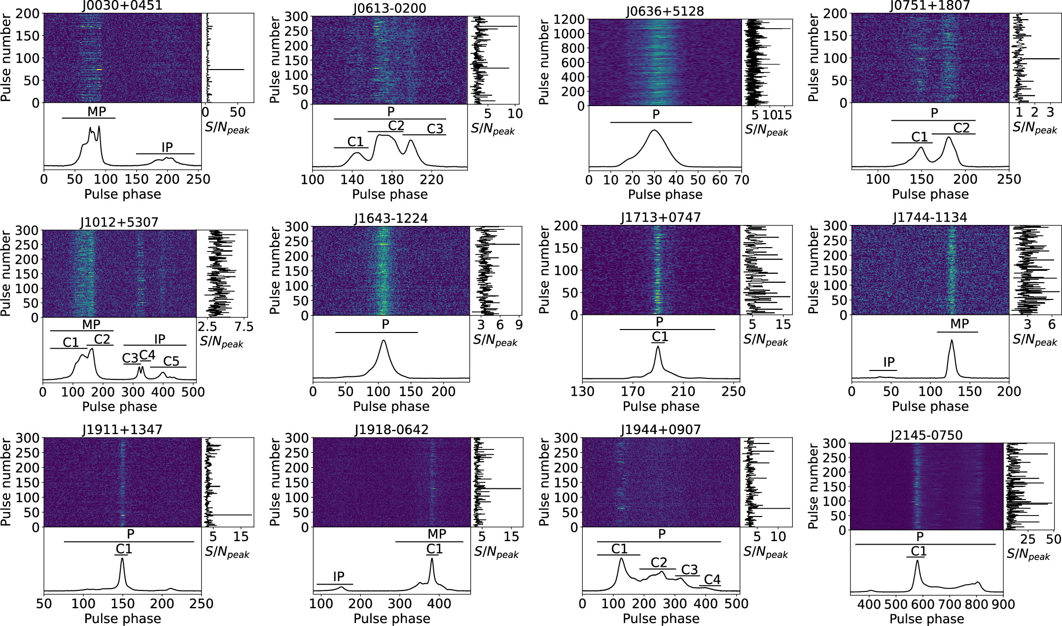
We present the single-pulse stacks for these 12 pulsars in Figure 4. It is worth noting that there are some bright pulses with narrow pulse widths. Therefore, we define the S/N_peak of a single pulse as I_peak/σ_off, where I_peak represents the peak intensity of a single pulse in the on-pulse region and σ_off is the rms of the off-pulse region. The S/N_peak of the single pulse versus pulse number for each pulsar is shown in the right panels of Figure 4, and the average profile of the entire observation is presented in the lower panels of Figure 4. We find that the single pulses in MSPs are unstable and exhibit significant variations in S/N_peak.

Zoom In Zoom Out Reset image size

To investigate the pulse intensity modulation behavior, we conduct a longitude-resolved fluctuation spectrum (LRFS; Backer 1970; Weltevrede 2016) analysis. Using the PSRSALSA package (Weltevrede 2016), we obtain the LRFS for each pulsar, and we observe that 10 pulsars exhibit periodic intensity modulations, as shown in Figure 5. In the side panels of Figure 5, the spectra of the horizontally integrated LRFS are presented, where the vertical axis is measured in cycles per period (P/P₃) with the vertical band separation P₃. The peak of the side panel corresponds to the modulation period of the pulse intensity. Following the method of Weltevrede (2016), if the vertical extension of P₃ is smaller than 0.05 cycles per period, it is defined as coherent modulation; otherwise, it belongs to diffuse modulation.

Zoom In Zoom Out Reset image size

The modulation periods of the pulse intensities for the pulsars are shown in Table 3. There are 10 pulsars that exhibit periodic intensity modulations, namely: PSR J0030+0451, PSR J0613−0200, PSR J0636+5128, PSR J0751+1807, PSR J1012+5307, PSR J1643−1224, PSR J1713+0747, PSR J1918−0642, PSR J1944+0907, and PSR J2145−0750, with six pulsars being reported for the first time. The periodic intensity modulations of PSR J1918−0642, PSR J1012+5307, PSR J2145−0750, and PSR J1713+0747 were previously reported by Edwards & Stappers (2003) and Liu et al. (2016), respectively, which are consistent with our results. The comparisons for these four pulsars to the previously published results are shown in the following subsections. PSR J0030+0451, PSR J0636+5128, and PSR J1944+0907 exhibit coherent modulations, while the remaining seven pulsars show diffuse modulations. The pulse intensity modulation periods of these pulsars range from ∼6 − 665 ms (∼2 − 128 P).

Table 3. Pulse Intensity Modulation Periods in 10 Pulsars

PSR	Component	Modulation Period (P)	Type
J0030+0451	MP	5.5 ± 0.1	Coherent
J0613−0200	C1	6 ± 1.	Diffuse
	C2	72.9 ± 0.4	Diffuse
J0636+5128	P	84.3 ± 0.9	Coherent
	LP	2.20 ± 0.01	Coherent
	TP	2.20 ± 0.01	Coherent
J0751+1807	MP	128.0 ± 0.1/9.4 ± 0.1	Diffuse
	MP	6.3 ± 0.1	Diffuse
J1012+5307	C1	7.1 ± 0.1	Diffuse
	C2	7.1 ± 0.1	Diffuse
	C3/C4	11.1 ± 0.1	Diffuse
J1643−1224	P	46 ± 1	Diffuse
J1713+0747	C1	6.2 ± 0.1	Diffuse
J1918−0642	C1	3.3 ± 0.1	Diffuse
J1944+0907	C1/C2/C3	128 ± 2	Coherent
J2145−0750	C1	3.9 ± 0.1/ 2.0 ± 0.1	Diffuse

Download table as:  ASCIITypeset image

3.3.1. PSR J0030+0451

PSR J0030+0451 exhibits a main pulse (MP) and a relatively weak interpulse (IP; Figure 4). The energy distribution of the MP is shown in Figure 6, where the pulse energy is calculated across the on-pulse region labeled as MP in Figure 4. This distribution exhibits two peaks, which can be fitted by combination of a Gaussian function and a log-normal function, corresponding to the weak and bright modes, respectively. The Gaussian and log-normal functions intersect at approximately 2〈E〉 (marked by the vertical red line in Figure 6). To identify the two modes, we employ a criterion where a single pulse with energy greater than 2〈E〉 is classified as belonging to the bright mode, otherwise, it is assigned to the weak mode.

Zoom In Zoom Out Reset image size

In Figure 7, the averaged profiles of the weak and bright modes are presented. In the bright mode, the profile exhibits a significantly stronger MP compared to the weak mode, while the IPs have the same shape and flux density in both modes. LRFS analysis reveals that the MP shows periodic intensity modulations, with a period of 5.5 ± 0.1 P, whereas no such periodic modulations are observed in the IP (Figure 5). The periodic modulation spans the entire profile of the MP. We conclude that PSR J0030+0451 exhibits a periodic mode-changing phenomenon, which has never been reported in MSPs before.

Zoom In Zoom Out Reset image size

We also note that the maximum energy of the MP exceeds 10〈E〉, which suggests the existence of giant pulses. The profile of the brightest pulse is shown in Figure 8, with a W50 width of 58 μs, much narrower than the average pulse of 577 μs. The energy and peak intensity of this pulse are about 11 and 70 times greater than the average pulse, respectively. PSR J0030+0451 might be a potential giant pulse emitter. However, due to the limitations of our observation with an 8.192 μs interval, it is insufficient to identify typical giant pulses with nanosecond durations. Further observations with a higher sampling interval are required.

Zoom In Zoom Out Reset image size

The measured σ_J(h) at different frequencies for previously reported results are shown in Figure 2, where there is a tendency for the jitter noise to increase with observing frequency. Our measured σ_J(h) is 43.4 ± 0.1 ns at 1250 MHz, which is smaller than the results of 60 ns at 1284 MHz (Parthasarathy et al. 2021), 153 ns at 1400 MHz (Lam et al. 2016), and ${61.1}_{-3.5}^{+3.5}$ ns at 1500 MHz (Lam et al. 2019). Therefore, it is reasonable that our measured jitter noise at 1250 MHz is smaller than the reported values at higher observing frequencies.

3.3.2. PSR J0613−0200

PSR J0613−0200 exhibits three components, namely C1, C2, and C3 (Figure 4). Among these components, C2 exhibits greater flux density compared to C1 and C3. We perform LRFS analysis for this pulsar, and the results are presented in Figure 5. We detect periodic modulations across the C1 and C2 components, with modulation periods of 6 ± 1 P and 72.9 ± 0.4 P, respectively.

The measured σ_J(h) at different frequencies for previously reported results are shown in Figure 2. Similar to the case of PSR J0030+0451, there is also a tendency for the jitter noise to increase with observing frequency for PSR J0613−0200. Our measured σ_J(h) is 34.4 ± 0.2 ns at 1250 MHz, which roughly agrees with the results of <400 ns at 1400 MHz (Shannon et al. 2014) and of <44 ns at 1400 MHz (Lam et al. 2016), but is much smaller than the result of ${133}_{-8}^{+8}$ ns at 1500 MHz (Lam et al. 2019).

3.3.3. PSR J0636+5128

PSR J0636+5128 exhibits a single component in its pulse profile (Figure 4). The pulsar exhibits complicated periodic modulations (Figure 5). A modulation period of 84.3 ± 0.9 P occurs across the entire profile, while modulation periods of 2.20 ± 0.01 P and 2.26 ± 0.01 P occur only in the leading and trailing parts of the profile, respectively.

The measured σ_J(h) at different frequencies for previously reported results are shown in Figure 2. Our measured σ_J(h) is 29.6 ± 0.4 ns at 1250 MHz, which is smaller than the results of ${62}_{-22}^{+16}$ ns at 1500 MHz and ${47}_{-11}^{+13}$ ns at 820 MHz (Lam et al. 2019), but with much smaller uncertainties.

3.3.4. PSR J0751+1807

PSR J0751+1807 exhibits two components, C1 and C2, with C2 being stronger (Figure 4). The bright single pulses occur across both the C1 and C2 components (Figure 4). We perform LRFS analysis and find periodic modulations in both components (Figure 5). The modulation period of C1 is 128.0 ± 0.1 P, while the modulation period of C2 is 6.3 ± 0.1 P. The correlation coefficient between the energy of the two components is 0.35, indicating no significant correlation between them. We report a new jitter measurement of this pulsar with σ_J(h) = 32.5 ± 0.5 ns.

3.3.5. PSR J1012+5307

PSR J1012+5307 exhibits an MP and an IP in its pulse profile (Figure 4). The pulsar presents complex modulations in both the MP and IP (Edwards & Stappers 2003). Our highly sensitive observation allows for a more detailed study of the modulations (Figure 4). By calculating the LRFS, we find that the two components of the mean pulse (C1 and C2) exhibit different modulation periods, with modulation periods of 7.1 ± 0.1 P and 7.6 ± 0.1 P, respectively. For the IP, periodic modulations are observed only in the first and second components (C3 and C4), with a similar modulation period of 11.1 ± 0.1 P.

The measured σ_J(h) at different frequencies for previously reported results are shown in Figure 2, showing a tendency for the jitter noise to increase with observing frequency. Our measured σ_J(h) is 27.0 ± 0.2 ns at 1250 MHz, which roughly agrees with the result of <103 ns at 1400 MHz (Lam et al. 2016), but is smaller than the result of 67 ± 6 ns at 1500 MHz (Lam et al. 2019).

3.3.6. PSR J1643−1224

PSR J1643−1224 exhibits a single component in its pulse profile (Figure 4). The pulsar exhibits periodic modulation, with a period of 46 ± 1 P occurring across the leading part of the profile, as determined by LRFS analysis (Figure 5).

The measured σ_J(h) at different frequencies for previously reported results are presented in Figure 2, showing a tendency for the jitter noise to increase with observing frequency. Our measured σ_J(h) is 40.8 ± 0.3 ns at 1250 MHz, which roughly agrees with the results of <60 ns at 1284 MHz (Parthasarathy et al. 2021) and <500 ns at 1400 MHz (Shannon et al. 2014), but is smaller than the results of 155 ns at 1400 MHz (Lam et al. 2016) and ${120}_{-10}^{+8}$ ns at 1500 MHz (Lam et al. 2019).

3.3.7. PSR J1713+0747

PSR J1713+0747 is a bright MSP. The profile of the pulsar changed between 2021 April 15 and 2021 April 17 (Xu et al. 2021), and shows a slow recovery continuing for the last several years (Jennings et al. 2022). Our observation was on 2021 August 20, during which the profile had not yet completely recovered. PSR J1713+0747 exhibits multiple components, but is dominated by a central component (C1) in its pulse profile (Figure 4). We identified a periodic modulation in our observation, with a period of 6.2 ± 0.1 P (Figure 5). Considering the diffuse modulation, we think that our result is roughly consistent with the previous result of 6.9 ± 0.1 P reported by Liu et al. (2016).

The measured σ_J(h) at different frequencies for previously reported results are shown in Figure 2, where there is a tendency for the jitter noise to decrease with observing frequency. Our measured σ_J(h) is 24.9 ± 0.3 ns at 1250 MHz, which is smaller than the results of 35.0 ± 0.8 ns at 1400 MHz (Shannon et al. 2014), 28/36 ns at 1400 MHz (Lam et al. 2016), and ${29.3}_{-0.9}^{+3.2}$ ns at 1500 MHz (Lam et al. 2019). Note that the profile in our observation has not recovered yet, which may cause the change in the level of jitter noise. For pulsars exhibiting mode-changing phenomena, the levels of jitter noise in different modes can vary, as seen in PSR J1909−3744 (Miles et al. 2022).

3.3.8. PSR J1744−1134

PSR J1744−1134 exhibits an MP and a weak IP in its pulse profile (Figure 4). The measured σ_J(h) at different frequencies for previously reported results are shown in Figure 2, indicating a pattern of the jitter noise decreasing and then increasing with observing frequency. Our measured σ_J(h) is 29.4 ± 0.2 ns at 1250 MHz, which agrees with the results of 31 ns at 1400 MHz (Lam et al. 2016) and 30 ± 6 ns at 1284 MHz (Parthasarathy et al. 2021), but is smaller than the results of 37.8 ± 0.8 ns at 1400 MHz (Shannon et al. 2014) and 46.5 ± 1.3 ns at 1500 MHz (Lam et al. 2019).

3.3.9. PSR J1911+1347

PSR J1911+1347 exhibits a relatively bright pulse component (C1) surrounded by broader emission in its pulse profile (Figure 4). The narrow bright pulses primarily occur in the C1 component. The measured σ_J(h) at different frequencies for previously reported results are shown in Figure 2, showing an increase in jitter noise with observing frequency. Our measured σ_J(h) is 27.8 ± 0.2 ns at 1250 MHz, which is smaller than the result of ${43.5}_{-2.3}^{+2.3}$ ns at 1500 MHz (Lam et al. 2019).

3.3.10. PSR J1918−0642

PSR J1918−0642 exhibits an MP and an IP in its pulse profile. The MP exhibits a relatively bright pulse component (C1) with broader emission flanking it, and the narrow bright pulse only occurs in C1 (Figure 4). Previous work by Edwards & Stappers (2003) suggested that PSR J1918−0642 may exhibit quasiperiodic modulations, with periods ranging from 2 to 4 P, but the limited sensitivity of their study made their results uncertain. In our analysis, we detected periodic modulation in this pulsar, with a period of 3.3 ± 0.1 P, through the calculation of the LRFS (Figure 5). However, the modulation only occurs across C1 of the MP.

The measured σ_J(h) at different frequencies for previously reported results are shown in Figure 2, with the jitter noise increasing as the observing frequency increases. Our measured σ_J(h) is 55.7 ± 0.5 ns at 1250 MHz, which agrees with the results of <101 ns at 1400 MHz (Lam et al. 2016), ${56}_{-13}^{+9}$ ns at 1500 MHz (Lam et al. 2019), and <55 ns at 1284 MHz (Parthasarathy et al. 2021).

3.3.11. PSR J1944+0907

PSR J1944+0907 exhibits a wide profile, with about four components (C1, C2, C3, and C4) in its pulse profile (Figure 4). The bright narrow single pulse is primarily observed in C1. We identified a periodic modulation that occurs across the C1, C2, and C3 components, with the same modulation period of 128 ± 2 P, by calculating the LRFS (Figure 5).

The measured σ_J(h) at different frequencies for previously reported results are shown in Figure 2, with the jitter noise increasing as the observing frequency increases. Our measured σ_J(h) is 174 ± 1 ns at 1250 MHz, which is smaller than the results of 196 ns at 1400 MHz (Lam et al. 2016) and ${311}_{-7}^{+6}$ ns at 1500 MHz (Lam et al. 2019).

3.3.12. PSR J2145−0750

PSR J2145−0750 is a bright MSP with multiple components in its pulse profile (Figure 4). We observed a periodic modulation occurring across the C1 component, with a modulation period of 3.9 ± 0.1 P (Figure 5), which is consistent with the previous result of ∼2 − 4 P (Edwards & Stappers 2003).

The measured σ_J(h) at different frequencies for previously reported results are shown in Figure 2, where no obvious tendency of an increase/decrease with observing frequency is detected. Our measured σ_J(h) is 168 ± 1 ns at 1250 MHz. This value agrees with the result of ${173}_{-4}^{+3}$ ns at 1500 MHz (Lam et al. 2019), but is larger than the result of 85 ns at 1400 MHz (Lam et al. 2016) and smaller than the results of 192 ± 6 ns at 1400 MHz (Shannon et al. 2014) and 200 ± 20 ns at 1284 MHz (Parthasarathy et al. 2021).

3.4. Timing a Subselection of Single Pulses

The variability of single pulses introduces jitter noise, which can have a significant impact on highly sensitive observations. It may be possible to improve the timing precision by selecting a subset of single pulses. Miles et al. (2022) conducted a timing analysis on PSR J1909−3744, which shows a mode-changing phenomenon, and found that the timing precision improved by approximately 10% by only timing the strong mode. Osłowski et al. (2014) studied the rms of the timing residual of PSR J0437−4715 for average profiles formed by integrating for 1 minute, but rejecting the brightest single pulses with different S/Ns. They found that the rms of the timing residual decreases with the increasing S/N, but no significant improvement is achievable. Following the method of Osłowski et al. (2014), we divided the observation into several segments, each lasting 60 s. Within each segment, we separately summed all the pulses, as well as the bright and weak pulses. We then formed three pulse templates based on the average profiles of the bright, weak, and all the pulses from the entire observation, using PAAS. Pulse ToAs were obtained by cross-correlating the summed profiles of the segments with the corresponding standard template, and timing residuals were calculated using the TEMPO2 software (a similar method was demonstrated in Wang et al. 2020). We consider a timing precision improvement to be achievable if the weighted rms (Wrms) of the timing residuals obtained using a subselection of pulses is lower than that obtained using all of the pulses.

We note that there are some bright pulses with narrow-pulse-width pulsars (Figure 4). Therefore, we use S/N_peak to define the bright pulses. We define a threshold value (S/N_crit) to classify the pulses as either bright or weak. If the S/N_peak of a single pulse is greater than S/N_crit, it is classified as a bright pulse; otherwise, it is classified as a weak pulse. For each pulsar, we divide the single pulses into five groups, based on S/N_crit (Table 4). Here, S/N_mean represents the mean S/N_peak, while ${\rm{S}}/{{\rm{N}}}_{\max }$ and ${\rm{S}}/{{\rm{N}}}_{\min }$ are the maximum and minimum S/N_peak values, respectively. We then calculate the Wrms of the timing residuals for the bright and weak pulses at these five S/N_crit values for each pulsar (Figure 9). As the number of bright pulses decreases with increasing S/N_crit, it is expected that the Wrms of the bright pulses will increase (the red lines in Figure 9), while that of the weak pulses will decrease (the blue lines in Figure 9). However, when comparing the timing precision achieved using a subset of pulses with a specific range of S/N_peak to the timing precision achieved using all of the single pulses (the black lines in Figure 9), we did not observe an improvement in timing precision for the pulsars in our sample, just like the case of PSR J0437−4715 (Osłowski et al. 2014).

Zoom In Zoom Out Reset image size

Table 4. The Threshold Values (S/N_crit) That Are Used to Classify the Bright/Weak Pulses

Groups	S/Ncrit
1	${\rm{S}}/{{\rm{N}}}_{\mathrm{mean}}-2/3(S/{N}_{\mathrm{mean}}-S/{N}_{\min })$
2	${\rm{S}}/{{\rm{N}}}_{\mathrm{mean}}-1/3(S/{N}_{\mathrm{mean}}-S/{N}_{\min })$
3	S/Nmean
4	${\rm{S}}/{{\rm{N}}}_{\mathrm{mean}}+1/3(S/{N}_{\max }-S/{N}_{\mathrm{main}})$,
5	${\rm{S}}/{{\rm{N}}}_{\mathrm{mean}}+2/3(S/{N}_{\max }-S/{N}_{\mathrm{main}})$

Download table as:  ASCIITypeset image

We have presented measurements of jitter noise, radiometer noise, and scintillation noise for 12 MSPs that are part of the IPTA sample, using FAST. In our analysis, we have determined that the mean levels of jitter noise, radiometer noise, and scintillation noise in a 1 hr duration are approximately 58 ns, 33 ns, and 4 ns, respectively. This indicates that the contribution of scintillation noise is likely negligible, being roughly one-tenth the level of the jitter/radiometer noise, consistent with previous published results (e.g., Lam et al. 2016). Our results suggest that jitter noise significantly contributes to white noise, emphasizing its notable impact on PTA observations with FAST.

Jitter noise is known to exhibit frequency dependence (Lam et al. 2019). When considering previously published results on jitter noise, we observe a diverse trend: while the jitter noise for some pulsars increases with observing frequency, it decreases for others. Lam et al. (2019) conducted a comprehensive analysis of the frequency dependence of the jitter noise in a large sample of MSPs, revealing a wide range of indexes in a power-law model, spanning from −3.2 to 9. MSPs typically demonstrate simple power-law spectra with a mean index of approximately −1.67 (Dai et al. 2015), resulting in radiometer noise increasing with observing frequency. For pulsars, the interplay between jitter noise and radiometer noise at varying observing frequencies becomes crucial. If the jitter noise increases with frequency, exhibiting a spectrum steeper than the radiometer noise, it dominates at higher frequencies; otherwise, the radiometer noise prevails. Optimizing observations can be achieved through the use of multiple telescopes with distinct observing frequencies. For instance, higher-frequency observations for specific pulsars might significantly improve the arrival time precision (Lam et al. 2018). The Qitai Radio Telescope (QTT), currently under construction, will enable high-sensitivity observations spanning from 150 MHz up to 115 GHz (Wang et al. 2023). The synergy between FAST and QTT will promise a substantial contribution to the capabilities of PTAs.

Our results indicate the substantial impact of jitter noise on PTAs with FAST. The investigation of single pulses represents a potential avenue for improving the timing precision of MSPs. For instance, Miles et al. (2022) conducted a timing analysis on PSR J1909−3744, which exhibits a mode-changing phenomenon. They observed an approximately 10% improvement in the timing precision by exclusively considering the strong mode. In our sample, where some pulsars exhibit bright and narrow single pulses or periodic intensity modulations, we have explored the potential for improving the timing precision by selecting specific subsets of single pulses. However, our analysis revealed that selecting a subset based on a specific range of S/N_peak did not improve the achievable timing precision.

To improve the pulsar timing precision, considering information about polarized radiation has been proposed (van Straten 2006; Osłowski et al. 2013). Accordingly, we conducted matrix template matching using all four Stokes parameters (van Straten 2006) for each pulsar to generate pulse ToAs, and measured radiometer and jitter noise. We successfully detected jitter noise in eight pulsars. Notably, we observed a decrease in jitter noise, ranging from 6.7% to 39.6%, while radiometer noise increased by 6.1%–38.6%. The total white noise also decreased for seven out of the eight pulsars in our sample, ranging from 0.19% to 13.4%. Therefore, matrix template matching using all four Stokes parameters is a valuable method for reducing jitter noise in pulsars. In future work, we plan to generate pulse ToAs by considering all four Stokes parameters on a large data set of MSPs using FAST, and present the noise analysis of them with the expectation of further improving the pulsar timing precision.

The highly sensitive and rapidly sampled observations conducted with FAST have provided us with the opportunity to study single pulses in a larger sample of MSPs. Utilizing LRFS analysis, we identified periodic intensity modulations in 10 pulsars: PSR J0030+0451, PSR J0613−0200, PSR J0636+5128, PSR J0751+1807, PSR J1012+5307, PSR J1643−1224, PSR J1713+0747, PSR J1918−0642, PSR J1944+0907, and PSR J2145−0750. Notably, six of these pulsars were reported for the first time. Our findings for PSR J1918−0642, PSR J1012+5307, PSR J2145−0750, and PSR J1713+0747 are consistent with previous results from Edwards & Stappers (2003) and Liu et al. (2016). PSR J0030+0451, PSR J0636+5128, and PSR J1944+0907 exhibit coherent periodical modulations, whereas the remaining seven pulsars show diffuse periodical modulations. The modulation periods for these MSPs range from approximately 6 to 665 ms (2 to 128 P), which is notably shorter than those observed in normal pulsars, typically ranging from a few seconds to several minutes (Basu et al. 2020). The origin of the periodic modulations in normal pulsars and MSPs remains unknown. In normal pulsars, these modulations are attributed to global changes in currents within the pulsar magnetosphere (Latham et al. 2012) and are generally observed across the entire pulse profile (Basu et al. 2020). Some normal pulsars exhibit phase-locked modulations of the MP and IP (Weltevrede et al. 2007). However, in MSPs, periodic modulations may occur only across a portion of the profile. We did not observe phase-locked phenomena in MSPs with IP emission. For example, in PSR J1012+5307, the modulation periods of the MP and IP are different. In PSR J0030+0451, periodic modulation is only detected in the mean pulse. The distinct modulation characteristics between MSPs and normal pulsars may be attributed to the presence of multiple emission regions in the magnetospheres of MSPs, with different pulse components originating from distinct locations (e.g., Dyks et al. 2010).

In particular, we identified brighter, narrower single pulses in PSR J0030+0451, with energies exceeding 10 times the mean pulse energy. This strongly suggests the presence of giant pulses. Additionally, we observed a periodic mode-changing phenomenon in PSR J0030+0451, a behavior not previously reported in MSPs. Until now, mode-changing phenomena have only been detected in two MSPs, namely PSR B1957+20 (Mahajan et al. 2018) and PSR J1909−3744 (Miles et al. 2022). However, the mode cycles observed in PSR B1957+20 and PSR J1909−3744 are not periodic. Further observations with FAST, encompassing a larger sample of MSPs, may unveil more instances of diverse emission behaviors, such as mode changing, nulling, or giant pulses. This expanded data set could provide valuable constraints on the emission properties of MSPs.

This work is supported by the National Natural Science Foundation of China (No. 12288102, No. 12203092, and No. 12041304), the Major Science and Technology Program of Xinjiang Uygur Autonomous Region (No. 2022A03013-3 and No. 2022A03013-2), the National SKA Program of China (No. 2020SKA0120100), the National Key Research and Development Program of China (No. 2022YFC2205202 and No. 2021YFC2203502), the Natural Science Foundation of Xinjiang Uygur Autonomous Region (No. 2022D01B71, No. 2022D01D85, and No. 2022D01D85), the Tianshan Talent Training Program for Young Elite Scientists (No. 2023TSYCQNTJ0024) and the Special Research Assistant Program of CAS, the CAS Project for Young Scientists in Basic Research (No. YSBR-063), the Key Research Project of Zhejiang Laboratory (No. 2021PE0AC03), and the Zhejiang Provincial Natural Science Foundation of China, under grant No. LY23A030001. This work has made use of data from the Five-hundred-meter Aperture Spherical radio Telescope, which is a Chinese national megascience facility, operated by the National Astronomical Observatories, Chinese Academy of Sciences. This research is partly supported by the Operation, Maintenance and Upgrading Fund for Astronomical Telescopes and Facility Instruments, budgeted from the Ministry of Finance of China (MOF) and administered by the Chinese Academy of Sciences (CAS).

Software: DSPSR (van Straten & Bailes 2011), PSRCHIVE (Hotan et al. 2004), TEMPO2 (Hobbs et al. 2006), and PSRSALSA (Weltevrede 2016).