


Abstract
The nearly 33 yr long-term radio light curve obtained with the Metsähovi Radio Observatory 14 m telescope at 37 GHz and the recent 12.7 yr γ-ray light curve of the blazar S5 0716+714 at 0.1–300 GeV from the Fermi Large Area Telescope (Fermi-LAT) were analyzed by using the Lomb–Scargle periodogram and the weighted wavelet Z-transform techniques. In the radio light curve, we discovered a possible quasi-periodic oscillation (QPO) signal of about 352 ± 23 days at a confidence level of ∼3σ. We recalculated the periodicity and its significance in a chosen time range that has higher variability and denser sampling, and then found that the significance had increased to a confidence level of 99.996% (∼4.1σ). This QPO component was further confirmed by fitting a linear autoregressive integrated moving average model to the selected radio light curve. A possible QPO of 960 ± 80 days at a 99.35% level (∼2.7σ) was found in the γ-ray light curve, which generally agrees with the earlier QPO claims of S5 0716+714. This paper discusses possible mechanisms for this potential year-like QPO. One possibility is a pure geometrical scenario with blobs moving helically inside the jet. Another is a supermassive binary black hole involving a gravitational wave-driven regime. In the latter scenario, we derived a milliparsec separation in the binary system that undergoes coalescence within a century due to the emission of low-frequency gravitational waves.
Export citation and abstract BibTeX RIS

Original content from this work may be used under the terms of the Creative Commons Attribution 4.0 licence. Any further distribution of this work must maintain attribution to the author(s) and the title of the work, journal citation and DOI.
1. Introduction
Active galactic nuclei (AGNs) belong to the most energetic extragalactic sources in the universe. Their bolometric luminosity is in the range of 1041–1048 erg s−1. They are widely believed to be powered by the accretion process of supermassive black holes (SMBHs), which range between 106 and 1010 M⊙ (e.g., Urry & Padovani 1995). Under the unified AGN paradigm, blazars belong to the most luminous and violently variable subclass. They show some remarkable properties, such as large amplitude and rapid emission in all spectral bands, strong and irregular polarization at radio and optical energies, the apparent superluminal motion of radio emission, and core-jet radio morphologies (Ulrich et al. 1997). Their nonthermal intense continuum emissions are predominantly dominated by the relativistic jets. These emissions could be created as the jets are aligned at close angles (≤10°) with the line of sight.
Across the entire electromagnetic spectrum, blazars are known to be variable on diverse timescales, ranging from a few minutes through weeks to years. Different timescales are thought to be associated with different physical processes. Short-term variability, from minutes to hours, for instance, might be produced in inner emission regions that are affected by the black hole gravity, while long-term variability, from months to years, is thought to be related to the jet structure itself or other geometrical effects (e.g., Gupta et al. 2017). Most of the timing analyses of blazar light curves demonstrate that the blazar emissions on different timescales are apparently chaotic and stochastic, which might mean that the underlying noise process governs the signal.
However, periodic or quasi-periodic oscillations (QPOs) have attracted the attention of academics for decades. They can benefit our understanding of the dynamical process occurring in the central engines of blazars. QPOs on an intra-day timescale can generally originate from the accretion disk fluctuations or oscillations, e.g., orbiting hotspots on the accretion disk or accretion disk pulsation (e.g., Gupta et al. 2009; Lachowicz et al. 2009; Kaur et al. 2017). In contrast, QPOs on a timescale longer than months are usually attributed to supermassive binary black hole (SMBBH) systems. The multiplicity, transient nature, and harmonic relation of the QPOs from different electromagnetic bands could be a powerful diagnostics of dynamic processes associated with blazars (e.g., Ciprini et al. 2007; Wang et al. 2014; Bhatta 2017; Tripathi et al. 2021).
S5 0716+714 is one of the brightest and most active blazars at radio frequencies at a redshift z = 0.31 ± 0.08 (Nilsson et al. 2008), discovered in a 5 GHz extragalactic radio source survey in 1979 (Küehr et al. 1981). It was first detected in the very high energy (VHE, >100 GeV) γ-ray band by MAGIC telescope during an optical flare in 2018 (Anderhub et al. 2009). It was classified as a BL Lac object. This subclass of blazars has a featureless spectrum and strong optical polarization. Even among blazars, S5 0716+714 is well known for its remarkable flaring behavior across the entire electromagnetic spectrum, and it has been the subject of several multiwavelength campaigns (e.g., Ostorero et al. 2006; Gupta et al. 2012; Liao et al. 2014; Chandra et al. 2015; Dai et al. 2015; MAGIC Collaboration et al. 2018). Since the intra-day variability (IDV) was detected for the first time simultaneously in the radio and optical wave bands in 1990 (Wagner et al. 1996), the attention is particularly focused on the search for and interpretation of the IDV (e.g., Montagni et al. 2006; Ostorero et al. 2006; Rani et al. 2010; Chandra et al. 2011; Dai et al. 2015; Man et al. 2016; Yuan et al. 2017; Liu et al. 2019; Dai et al. 2021, and references therein ). The variation rate was faster than 0.1–0.12 mag hr−1 (Montagni et al. 2006), even up to 0.38 mag hr−1 (Chandra et al. 2011), and the IDV timescale can be as short as 15 minutes (Rani et al. 2010) and 17.6 minutes (Man et al. 2016) in the optical-light wave bands. Moreover, this source showed rapid flaring activities on a timescale of a few hours to days, superimposed on a broad and slow variability trend on a timescale of ∼1 yr (Rani et al. 2013). However, the emission mechanism responsible for the broadband flaring activities is not yet well understood. Therefore, it is crucial to investigate whether the flaring components have recurring features and if flaring events at different frequencies are correlated, especially events at high and low energies. The flaring activities that might be associated with the QPO behavior of S5 0716+714 that has caught researchers' attention needs to be studied as well (e.g., Raiteri et al. 2003; Prokhorov & Moraghan 2017; Li et al. 2018a, 2018b; Bhatta & Dhital 2020).
Over the past few decades, several monitoring campaigns, such as Fermi-LAT 6 , the Astro-rivelatore Gamma a Immagini Leggero 7 (AGILE), Swift 8 , the Small and Moderate Aperture Research Telescope System 9 (SMARTS), the University of Michigan Radio Astronomical Observatory 10 (UMRAO), and the Metsähovi Radio Observatory program 11 , have been continuously performed to observe S5 0716+714 and released large amounts of data, which enable the search for QPO on long-term timescales. In this work, we study the γ-ray and radio variabilities of this source, including the detection of QPOs with a significance test and interpretation of candidate QPOs. Section 2 describes the observations and data reduction procedures. Section 3 outlines the analysis techniques and presents the detection of candidate QPOs against the red-noise background. Our final discussion is given in Section 4, and our conclusions are presented in Section 5.
2. Observations and Data Reduction
The 37 GHz observations between 1988 June 29 and 2021 May 3 (MJD 47342–59337) were made with the 13.7 m diameter Metsähovi radio telescope, operated by Aalto University, Finland. The detection limit of the telescope at 37 GHz is on the order of 0.2 Jy under optimal conditions. Data points with a signal-to-noise ratio <4 are handled as nondetections. The flux density scale is set by observations of DR 21. Sources NGC 7027, 3C 274 and 3C 84 are used as secondary calibrators. A detailed description of the data reduction and analysis is given in Teraesranta et al. (1998). The error estimate in the flux density includes the contribution from the measurement rms and the uncertainty of the absolute calibration. Long-term variabilities of Metsähovi monitoring data at 22 GHz, 37 GHz, and 87 GHz in a large sample of AGN were analyzed by Hovatta et al. (2007) using different statistical methods: periodogram, structure function, and discrete correlation function. Metsähovi data at 37 GHz of a sample of narrow-line Seyfert 1 galaxies were also used to look for detections and variability that would indicate the presence of radio jets (Lähteenmäki et al. 2017, 2018). Weekly averaged fluxes that smoothed short-term fluctuations of the light curves are presented in the bottom panel of Figure 1.

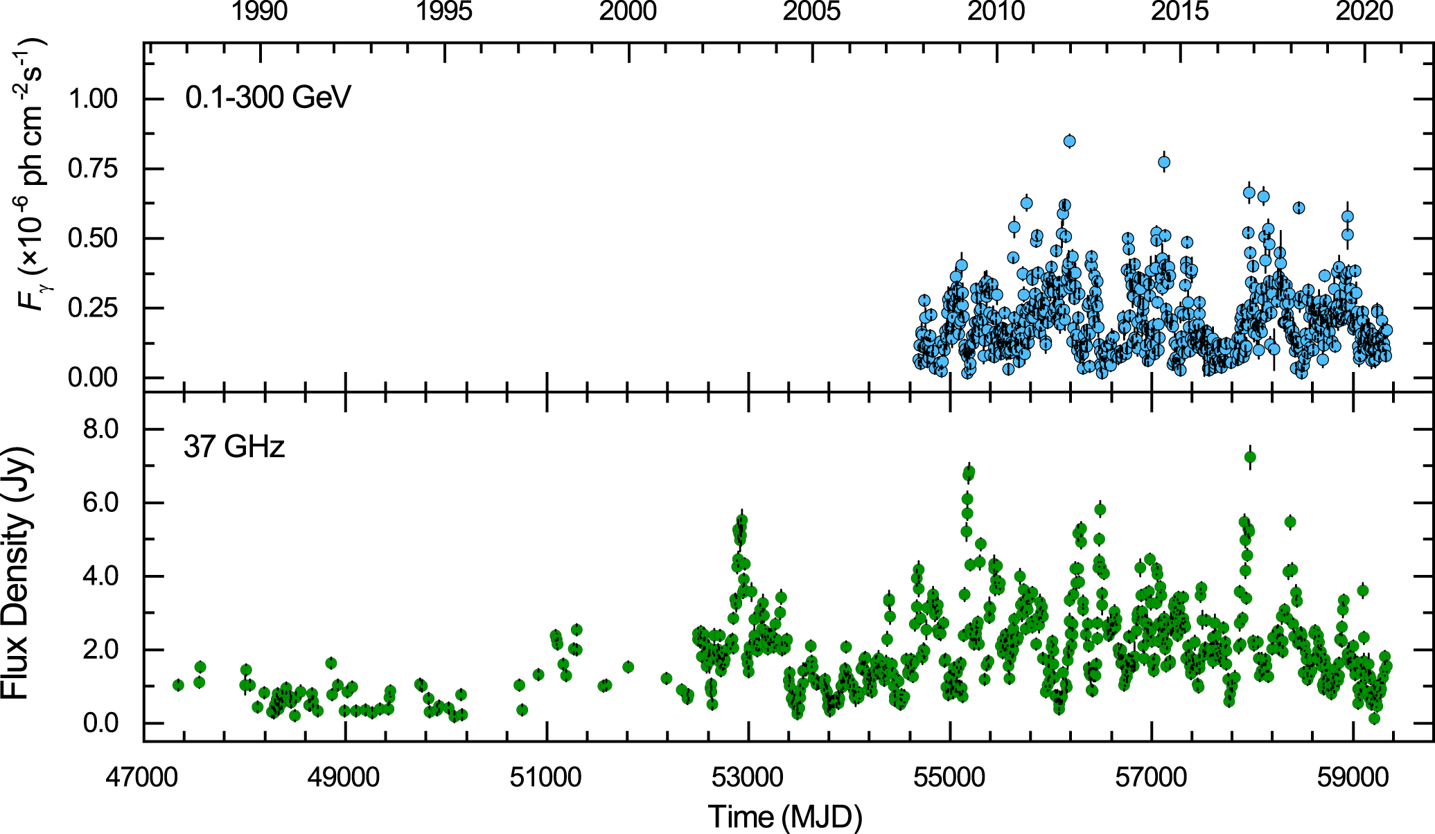
Figure 1. Weekly averaged light curves of the blazar S5 0716+714. Top panel: Fermi-LAT γ-ray light curve at 0.1–300 GeV from 2008 August 16 to 2021 May 1, spanning 12.7 yr, with TS>25. Bottom panel: Metsähovi light curve at 37 GHz from 1988 June 29 to 2021 May 3, spanning 32.8 yr.
Download figure:
Standard image High-resolution imageThe γ-ray fluxes in the energy range 0.1–300 GeV, between 2008 August 16 and 2021 May 1 (MJD 54694–59335), are obtained from the observation of the Fermi-LAT, following the standard procedure provided in the Fermi Science Support Center (FSSC). 12 The analysis was performed using the Fermitools version 2.0.8 and Pass 8 data. Photons were selected within a region of interest (RIO) with a radius of 15° centered on the source, using the tool gtselect with SOURCE event class (evclass = 128 and evtype = 3), and maximum zenith angle of 90°. We apply the recommended filter string "(DATA_QUAL > 0) && (LAT_CONFIG = = 1)" in the gtmktime tool to choose the good-time intervals. The source model file was created using the user-contributed tool make4FGLxml.py 13 based on the Fourth Fermi-LAT Source Catalog (4FGL; Abdollahi et al. 2020). This file included 276 sources within 20° centered at the center of the ROI. For each time bin, best-fitting results including flux, photon index, and test statistic (TS) value are derived with the tool gtlike using a binned likelihood analysis (see also, e.g., Abdo et al. 2009). Here, the normalizations and spectral parameters from all sources within 5° centered at the center of ROI and the normalizations of extragalactic diffuse backgrounds iso_P8R3_SOURCE_V3_v1.txt and gll_iem_v07.fits were set free. The significance of the source was described by a maximum likelihood test statistic TS = −2 ln(L0/L1), where L1 and L0 represent the maximum likelihood of the model value with and without the source, respectively. The γ-ray light curve was constructed using the detection criterion TS > 25 (∼5σ; (Mattox et al. 1996)) and a weekly bin, as shown in the top panel of Figure 1. A visual inspection of Figure 1 reveals that radio and γ-ray emissions are highly variable during the observation period, along with several separated flaring episodes.
3. Results
3.1. Periodicity Search
The weighted wavelet Z-transform (WWZ; Foster 1996) and the Lomb–Scargle periodogram (LSP; Lomb 1976; Scargle 1982) were employed to search for the periodicity in the radio and γ-ray light curves of S5 0716+714. Unlike LSP, the WWZ algorithm decomposes a time series into time and frequency space. It represents the WWZ power in the form of a contour plot, a color-scaled plot, or a 3D graph, in which periodic modulations and their evolution with time can be derived. The time-averaged WWZ power spectrum (the mean WWZ power at a given period) has been used to determine the periodic modulations without considering their evolution with time. A comparative analysis of these two methods has been widely used to search for possible QPO in blazar light curves, for example, Bhatta et al. (2016), Bhatta (2017), Zhang et al. (2017a), Zhang et al. (2017b), Zhou et al. (2018), Gupta et al. (2019), Sarkar et al. (2020), Sarkar et al. (2021), Li et al. (2021a), Li et al. (2021b), Zhang et al. (2021), and Roy et al. (2022).
The WWZ is based on a weighted projection onto three trial functions: ϕ1(t) = 1(t), ![${\phi }_{2}(t)=\cos [\omega (t-\tau )]$](https://content.cld.iop.org/journals/0004-637X/943/2/157/revision1/apjacae8cieqn1.gif) and
and ![${\phi }_{3}(t)\,=\sin [\omega (t-\tau )]$](https://content.cld.iop.org/journals/0004-637X/943/2/157/revision1/apjacae8cieqn2.gif) , and it also included statistical weights
, and it also included statistical weights  (α = 1, 2, 3) on the projection, where c is a constant that determines how rapidly the Morlet wavelet decays. The WWZ power estimates the significance of a detected periodicity with frequency ω and time shift τ in a statistical manner, i.e.,
where Neff indicates the effective number of data points contributing to the signal, and Vx and Vy are the weighted variations of the uneven data x and the model function y, respectively. These factors are defined as

In the denominators of Vx and Vy , parameter λ corresponds to the number of test frequencies. Analysis parameters, a limited frequency range of 0.00025–0.01 day−1, a period step of 10 days, and a decay constant c = 0.001 were adopted in the WWZ analysis, which enables a search for QPO on a timescale from several months to years and strikes a balance between frequency and time resolution.
In this paper, we first examine the existence of the periodic modulations for the whole radio and Fermi-LAT γ-ray light curves. The color contour of the WWZ power spectrum calculated for the 32.8 yr radio light curve is shown in the left part of the left panel in Figure 2. The figure reveals considerable WWZ power centered around 350, 850, 1300, 1800, and 2600 days. In the higher-frequency regimes, the remarkable periodicity of ∼350 days principally fluctuated in the middle and rear sections of the observations. The time-averaged WWZ power spectrum shown as the red curve (see the right part of the left panel in Figure 2) supports the above analyses, with distinct and remarkable power peaks centered at about 350 days, 850 days, 1300 days, 1800 days, and 2600 days. Furthermore, in the right part, the LSP power spectrum (dash–dotted blue curve) is generally consistent with the time-averaged WWZ power spectrum.
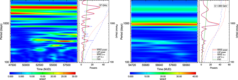
Figure 2. Search for QPOs in the radio and γ-ray light curves of S5 0716+714. Left panel: Color contour of the WWZ power spectrum for the whole radio light curve spanning 32.8 yr, time-averaged WWZ power spectrum (red curve), and the corresponding 3σ confidence level (dotted red curve), LSP power spectrum (dash–dotted blue curve) and the corresponding 3σ confidence level (dash–dot-dotted blue curve). The solid green line shows the best-fit underlying PSD with a bending power-law model. The significance test was evaluated by using the Python implementation provided by Connolly (2015) based on the method by Emmanoulopoulos et al. (2013). Right panel: Same as the left panel, but for the whole Fermi-LAT light curve spanning 12.7 yr.
Download figure:
Standard image High-resolution imageThe periodicity analysis for the 12.7 yr γ-ray light curve is shown in the right panel of Figure 2. Possible periodicities of about 350, 850, 1300, 1800, and 2600 days that fluctuated in the radio light curve cannot be derived from the WWZ color contour of the γ-ray light curve. However, a prominent periodicity of about 1000 days appears to be persistent throughout the whole observation, revealing some inconsistency in the periodic properties or different radiation mechanisms between radio and γ-ray emissions. As shown in the right part of the right panel, the periodic modulation of about 1000 days has also been revealed by both LSP power density curve and time-averaged WWZ power spectrum. A candidate QPO of ∼1000 days can therefore be derived from the positions of the WWZ and LSP power peaks.
3.2. Significance Estimation
Claims of QPOs in blazar light curves usually arouse the community's suspicions because the blazar flux variability is generally dominated by a frequency-dependent noise component (commonly known as red noise). This component can easily arise from stochastic processes in the accretion flows and jet plasma (e.g., Vaughan et al. 2016; Covino et al. 2019). Typically, the power spectral density (PSD) of a blazar light curve is well represented by a negative spectral index −α of the form P(f) ∝ f−α at the frequency f. This term indicates that the red-noise processes result in spurious spectral peaks in the periodograms and lead to misjudgments, especially in the lower-frequency domain. A useful approach to handle this issue is to evaluate the significance of potential spectral peaks against the red-noise background by simulating random light curves with a given power-law spectrum.
We simulated artificial light curves using the Python code DELightcurveSimulation
14
provided by Connolly (2015), based on the algorithm given by Emmanoulopoulos et al. (2013). The Emmanoulopoulos light-curve simulation algorithm represents an improvement of the procedure of Timmer & Koenig (1995), which reproduces light curves on the basis of the power spectral shape. Artificial light curves generated by this algorithm can preserve both the probability density function (PDF) and the underlying PSD of a original light curve. In this work, PSDs were derived by means of the normalized LSP due to the unevenly sampling of the weekly binned light curves. Since a pure power-law model only poorly described the PSDs simultaneously at low and high frequencies, we fit the PSDs of the light curve with a bending power-law model: ![$P(f)={{Af}}^{-\alpha }/\left[1+{\left(f/{f}_{\mathrm{bend}}\right)}^{\beta -\alpha }\right]+C$](https://content.cld.iop.org/journals/0004-637X/943/2/157/revision1/apjacae8cieqn4.gif) , where A, α, β, fbend, and C are the normalization, low-frequency slope, high-frequency slope, bend frequency, and Poisson noise level corresponding to the power, respectively. For this model, A, C, and fbend are all non-negative. The fit is obtained by finding the parameters of maximum likelihood using a Basin-Hopping algorithm and the Nelder-Mead minimization algorithm provided by the Python package SciPy (Virtanen et al. 2020). The corresponding fitted values for radio light curve are A = 0.72 ± 0.13, α = 0.35 ± 0.02, β = 3.05 ± 0.58, fbend =0.0061 ± 0.0005, and C = 0.42 ± 0.14, and for the γ-ray light curve, they are A = 8.60 ± 4.68, α = 0.01 ± 0.03, β = 1.82 ±0.30, fbend = 0.0027 ± 0.0007, and C = 0.49 ± 0.08. The reduced χ2 (
, where A, α, β, fbend, and C are the normalization, low-frequency slope, high-frequency slope, bend frequency, and Poisson noise level corresponding to the power, respectively. For this model, A, C, and fbend are all non-negative. The fit is obtained by finding the parameters of maximum likelihood using a Basin-Hopping algorithm and the Nelder-Mead minimization algorithm provided by the Python package SciPy (Virtanen et al. 2020). The corresponding fitted values for radio light curve are A = 0.72 ± 0.13, α = 0.35 ± 0.02, β = 3.05 ± 0.58, fbend =0.0061 ± 0.0005, and C = 0.42 ± 0.14, and for the γ-ray light curve, they are A = 8.60 ± 4.68, α = 0.01 ± 0.03, β = 1.82 ±0.30, fbend = 0.0027 ± 0.0007, and C = 0.49 ± 0.08. The reduced χ2 ( ) values of the fits are 7.32 for the radio light curve and 3.94 for the γ-ray light curve. The best-fit underlying PSDs for the radio and γ-ray light curves are shown in Figure 2, and the PDFs of the fluxes were fit using a log-normal distribution to histograms of the light curves.
Then, for each light curve, we simulated 106 light curves based on the fitting results of PSD and PDF from the original light curves. These artificial light curves have the same statistical properties, e.g., PSD, PDF, sampling, mean value, standard deviation, and the same gaps. The LSP and time-averaged WWZ power spectrum can be obtained for each simulated light curve. The confidence levels were estimated by using the percentiles of the power for each frequency in the periodograms of the simulated light curves, which means that the LSP and WWZ confidence levels were obtained from the simulated LSP and WWZ periodograms, respectively. In this work, a quasi-periodic signal in the periodograms was considered to be significant when its LSP power peak crossed the 3σ LSP confidence levels and the time-averaged WWZ power peak simultaneously crossed the 3σ WWZ confidence levels. As shown in Figure 2, the 3σ confidence curves evaluated from the artificial light curves are superimposed on the LSP and WWZ periodograms as dotted and dash–dot-dotted curved lines, respectively.
In the right part of the left panel in Figure 2, the remarkable LSP and WWZ power peaks centered at 850, 1300, 1800, and 2600 days did not reach the 3σ LSP and WWZ confidence levels simultaneously. In the right part of right panel evaluated for the γ-ray light curve, the possible QPO with high LSP and WWZ power amplitudes at 960 ± 80 days remained slightly below the 3σ LSP and WWZ confidence level. According to the confidence criterion mentioned above, the confidence of this possible QPO is not significant enough. If we averaged the the LSP and WWZ confidence levels at this periodicity, a confidence level of 99.35% could be derived. Nevertheless, this possible QPO signal lasted ∼4.8 cycles within ∼12.7 yr and generally agrees with the WWZ power evaluated for the Fermi-LAT light curve in Bhatta & Dhital (2020; top right panel in their Figure 6). Our analysis estimated the periodicity values and uncertainties by the peak positions and half-width at half maximum (HWHM) of the Gaussian function that fits the WWZ power peaks.
An inspection of the radio light curve (Figure 1) reveals that the source shows a higher variability and the data sample has a denser sampling starting from roughly MJD 52500 to the end of the observations. The fractional variability amplitude Fvar (as measured by the root mean square; Vaughan et al. 2003) and the average sampling rate of the radio light curve before MJD 52500 were calculated to be 0.52 ± 0.02 and 5.12 per yr, while after MJD 52500, they were calculated to be 0.63 ± 0.05 and 34.93 per yr, respectively. For the segmented radio light curve with denser sampling and stronger variability ranging from MJD 52496 to 59335, we recalculated the WWZ contour and the LSP power spectrum, fit the PSD with a bending power-law model, generated 106 light curves using the implementation of Emmanoulopoulos et al. (2013), and estimated the significance of the power peak. The fitted parameters of normalization, low-frequency slope, high-frequency slope, bend frequency, and Poisson noise are A = 0.027 ± 0.002, α = 0.876 ± 0.129, β = 1.026 ± 0.165, fbend = 0.0008 ± 0.0002, and C = 1.032 ±0.145, respectively, with  . In Figure 3, the WWZ and LSP analyses of the selected radio light curves reveal that the WWZ and LSP power peaks reach the corresponding 4σ confidence level, which means that the confidence levels of WWZ and LSP analysis have improved. The WWZ time-averaged power and LSP power strongly indicate the presence of a QPO of 352 ± 23 days above the 99.996% confidence level (∼4.1σ) against the red-noise background. Furthermore, at least 18 complete cycles are visible from the corresponding light curves and WWZ color contours. This is the first time that a QPO with a high significance level that lasted for sufficiently many cycles has been found in the radio light curve of S5 0716+714.
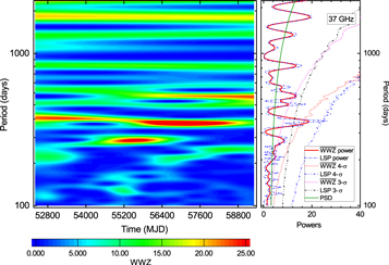
Figure 3. Same as Figure 2, but for the segmented time interval in the radio light curve discussed in Section 3.2, from 2009 September 13 to 2019 March 23 (MJD 54722–58565). The dotted red and magenta curves represent the 3σ and 4σ WWZ confidence level, respectively. The dash–dot-dotted blue and black curves represent the 3σ and 4σ LSP confidence level, respectively.
Download figure:
Standard image High-resolution image3.3. Light-curve Modeling
Blazar light curves can also be modeled by an autoregressive (AR) process. We further fit the selected radio light curve with an independent method called autoregressive integrated moving average (ARIMA) model (e.g., Zhang et al. 2017b; Feigelson et al. 2018; Caceres et al. 2019; Tarnopolski et al. 2020; Sarkar et al. 2021; Gong et al. 2022) to check the reliability of this year-like QPO signal and assess whether the time series is consistent with a stochastic origin of the AR noise. An ARIMA process combined an autoregressive (AR) process and a moving average (MA) process after differencing a nonstationary time series. Considering F(ti ) to be the emission at time ti , the analytical representation of the ARIMA(p, d, q) model is given by
where p, q, and d are the orders of AR, MA, and differencing, θ and ϕ represent the AR and MA coefficient, and L and  (ti
) are the lag operator and normally distributed random variable, respectively. ARIMA is one of the most frequently used models for evenly nonstationary time series, and differencing d times can remove the nonstationarity. For a quite general stationary time series, an ARIMA(p, d, q) process reduces to an ARMA(p, q) process with d = 0.
(ti
) are the lag operator and normally distributed random variable, respectively. ARIMA is one of the most frequently used models for evenly nonstationary time series, and differencing d times can remove the nonstationarity. For a quite general stationary time series, an ARIMA(p, d, q) process reduces to an ARMA(p, q) process with d = 0.
The even radio light curve covering the period MJD 52496–59335 was built with a 30-day binning, as shown in panel (a) of Figure 4. We performed an augmented Dickey-Fuller (ADF) test (Said & Dickey 1984) to test the nonstationarity of the 30-day binned light curve. The ADF test rejected the null hypothesis that a unit-root characteristic of a nonstationary process exists with a p-value < 0.001 and a test statistic−6.47, implying that the binned light curve exhibits stationary, and an ARIMA(p, 0, q) (or ARMA(p, q)) model can be applied to the light curve. Using the Akaike information criterion (AIC; Akaike 1974), we selected the optimum model by minimizing the AIC for ranges of p between 1 and 9 and q between 1 and 8. In panel (e) of Figure 4, we show the AIC heatmap for 72 ARIMA models fitting the 30-day binned radio light-curve segment. Obviously, the ARIMA (7,0,6) model with the minimum AIC value of 512.2 is the best-fit model.

Figure 4. Fitting results of S5 0716+714. Panel (a): 30-day binned radio light curve (MJD 52496–59335) and the best-fitting ARIMA(7,0,6) modeling results shown as a bright orange line. Panel (b): Standardized residuals from the fitted model. Panel (c): Distribution of the standardized residuals, as well as the best-fit normal distribution (red line). Panel (d): ACFs of the standardized residuals, compared with the 95% confidence limit of the white noise (dotted horizontal lines). Panel (e): AIC map for ARIMA(p, 0, q) models (p = 1,...,9 and q = 1,...,8) with darker shades corresponding to better models. The best model with the minimum AIC is bordered with a red square. Panel (f): Mean PSD assuming the ARIMA(7,0,6) model and the corresponding 2σ confidence interval (blue region) estimated from the Monte Carlo simulations.
Download figure:
Standard image High-resolution image
In Figure 4, panels (b) and (c) show the standard residuals and the corresponding probability density fitted with a normal distribution model, respectively. An Anderson-Darling (AD) test failed to reject the null hypothesis that the standard residuals stem from a population with a normal distribution at the 0.01 significance level. Panel (d) represents the autocorrelation function (ACF) of the residuals compared with the 95% confidence region assuming a white-noise process. We also performed a LjungBox test (Ljung & Box 1978) on the ACF to test the residual autocorrelation. The result failed to reject the null hypothesis that the residuals of the returns are not autocorrelated with p-value = 0.953, which is consistent with the result that no significant lags remain outside of the 95% limit in the ACF plot. Hence, the ARIMA (7,0,6) model is an appropriate fit to the selected 30-day binned light curve. We further simulated 104 light curves using the maximum likelihood parameter estimated from the partially specified ARIMA (7,0,6) model. The resulting mean PSD of the simulated light curves and the corresponding 2σ confidence intervals estimated from the modeling are shown in panel (f). A spike in the PSD at 0.0028 day−1 (∼350 days) is apparent, which agrees well with the spike found with the WWZ and LSP methods and indicates that the candidate QPO signal in the radio light curve may be intrinsic.
4. Discussion
As one of a few blazars claimed to exhibit QPOs, S5 0716+714 has shown distinctive quasi-periodic features in multiple wave bands with timescales ranging from more than 10 minutes through weeks to several years. Rani et al. (2010) first reported good evidence for a QPO of ∼15 minutes in S5 0716+714: the fastest QPO claimed in blazars at any wavelength in the optical band. Before then, a quasi-periodic IDV on timescales ranging between ∼25 minutes and ∼73 minutes was found by Gupta et al. (2009) via wavelet analysis in their optical IDV light curves, and Hong et al. (2018) also confirmed an optical QPO of ∼50 minutes at the 99% significance level. Candidate QPOs with timescales of ∼1 day appeared to be present in optical and radio bands simultaneously (Quirrenbach et al. 1991), and ∼4 days (Heidt & Wagner 1996), 14 days (Ma et al. 2004), ∼24 days (Yuan et al. 2017), and ∼60–70 days (Rani et al. 2013) have been detected in the optical emissions. S5 0716+714 also showed QPOs on a year-long timescale, e.g., a significant QPO of ∼340 days was found in the γ-ray light curves (Prokhorov & Moraghan 2017; Li et al. 2018a; Bhatta & Dhital 2020). For longer timescales, Raiteri et al. (2003) found QPOs of 3.0 ± 0.3 yr in the optical band and 5.5–6 yr in the radio band. The previous characteristic timescale is approximately consistent with a QPO with a period of ∼1000 days at a 99% significance level in both the optical and γ-ray bands (Bhatta 2021). The latter timescale generally agrees with the possible periodicity of ∼6.1 yr reported in Li et al. (2018b), who analyzed the UMRAO radio light curves using different techniques.
It can be seen that the existence of QPO in S5 0716+714 is now well established at different frequencies. However, some early periodicity claims were obviously overestimated due to the lack of a significance estimation and white-noise and/or red-noise background analyses. For instance, even though Prokhorov & Moraghan (2017) found a 340-day QPO in the Fermi-LAT γ-ray light curve, they neglected to take the random red-noise variations into account. In addition, Li et al. (2018a) reported a 266-day periodicity in 8.8 yr curves using the Jurkevich (Jurkevich 1971), LSP, and REDFIT (Schulz & Mudelsee 2002) methods. The significance of their QPOs was insufficient, however. Furthermore, it is quite unlikely that QPOs on different timescales have the same origin, and they may not even manifest at the same time at various wave bands, demonstrating the complexity of AGN QPOs. Therefore, any QPO claims in AGN should be verified with strict analysis.
In any case, our results reveal a year-like QPO (352 ± 23 days) at a 99.996% confidence level (∼4.1σ) in the 37 GHz light curve spanning ∼18.7 yr, which provides another intriguing instance among AGN QPO phenomena. Significantly, QPOs on year-like timescales have been searched from many multiwavelength light curves, and it appears that these QPOs seem to be frequent in blazars (e.g., Sandrinelli et al. 2014, 2016, 2018; Yang et al. 2021; Zhang et al. 2021, and references therein), although caution about the significance of some claimed QPOs detected at γ-rays has been expressed (e.g., Hovatta et al. 2007; Covino et al. 2019; Ait Benkhali et al. 2020). Recently, Sandrinelli et al. (2018) reconsidered their previous year-long QPO claims in the optical and γ-rays using different numerical schemes, and confirmed that year-like QPOs appeared in PKS 2155–304 and PG 1553+113. By applying multiple time-series analyses on the decade-long Fermi-LAT observations of 20 blazars, Bhatta & Dhital (2020) detected year-timescale QPOs in the sources S5 0716+714, Mrk 421, ON+325, PKS 1424–418, and PKS 2155–304. In a systematic search for γ-ray periodicity in more than 2000 AGNs proposed by Peñil et al. (2020), periodic emission around ∼0.9 yr (∼3σ) and ∼2.7 yr (nearly a multiple of 0.9 year) at a ∼3σ confidence level was found in S5 0716+714. Our analyses show a year-like QPO in the radio light curve of S5 0716+714, suggesting that year-like QPOs in blazars might be more frequent.
Additionally, our QPO analysis shows that there is no clear connection between radio and γ-ray emissions. To quantify the relative variability, we have calculated that Fvar for the whole radio and γ-ray light curves is 0.56 ± 0.01, and 0.64 ± 0.02, respectively. The γ-ray flux variability is more variable than the radio emission, which is consistent with the fact that the radio emission is expected to be produced by less compact regions on a larger jet scale, and the γ-ray photons are produced by inverse-Compton upscattering of low-energy synchrotron photons in the synchrotron-self-Compton (SSC) mechanism. Most recently, Kim et al. (2022) explored radio–γ-ray correlations and time lags of S5 0716+714 and found significant positive and negative correlations between radio and γ-ray activity in different time ranges, using the Metsähovi 37 GHz data, Fermi-LAT observations (0.1–200 GeV), Submillimeter Array (SMA) flux densities, and very long baseline interferometry (VLBI) data. In our work, both the WWZ and LSP power from the Fermi-LAT light curve provide evidence for a possible QPO of about 1000 days despite the lower significance and fewer duty cycles. However, such a QPO component could not stand out from the radio light curve in which a QPO of 352 ± 23 days was detected with high confidence. Both WWZ contours and periodograms for the radio and γ-ray light curve reveal the lack of a strict consistency between radio and γ-ray emissions and complicated physical processes in low- and high-energy radiation. This can be attributed to different radiative cooling timescales of electrons that emit synchrotron at raido frequencies and Compton emission at γ-ray frequencies, the passage of disturbances, or shocks moving through the radio cores, and/or influence from external or internal stochastic processes (e.g., Kim et al. 2022). Therefore, systematic studies of the quasi-periodic nature of multiwavelength light curves would be a powerful approach to constrain the connection among the multifrequency variabilities of blazars.
The current theoretical interpretations for blazar QPOs include accretion disk fluctuations, a disk-jet coupling scenario, a precessing jet scenario, helical jets or helical structures in jets, hydrodynamical instabilities in jets, SMBBH systems, or a combination of these. Relatively systematic summaries for the periodic driving scenario are provided by Ackermann et al. (2015) and Bhatta & Dhital (2020). There is no scientific consensus about the physical driving mechanism, however. Since the flux fluctuations are dominated by the relativistic jet, the periodic flux modulations in S5 0716+714 should be associated with internal mechanisms within the jet itself or with related processes powering the jet. Moreover, QPOs on short timescales may be due to accretion disk instabilities (e.g., Gupta et al. 2009; Lachowicz et al. 2009; Kaur et al. 2017). Therefore, as for the detected long-term QPOs in our analysis, the most balanced and reasonable scenario should be related to instabilities or structures in jets and dynamical interaction in a binary system. In the following content, the year-like QPO revealed for the first time in the radio light curve was assumed to be an existent periodic signal for a brief discussion of possible mechanisms.
S5 0716+714 is a jet-dominant source whose flux variabilities could be associated with the emission blobs, shock fronts, or perturbations propagating along with a precessing, bent, or helical jet. Here, we briefly discuss a geometrical scenario with enhanced emissions (or blobs) moving along the helical path of the jets (e.g., Mohan & Mangalam 2015; Sobacchi et al. 2017; Zhou et al. 2018; Sarkar et al. 2020, 2021). According to the inference from misalignment, precession, and wiggling of radio jets, a helical structure in a jet is usually expected to be intrinsic. When a blob that is injected near the base of the jet moves helically inside the jet with a high bulk Lorentz factor, the viewing angle θobs(t) of the helical motion of an emitting blob to the line of sight can be expressed as (e.g., Sobacchi et al. 2017; Zhou et al. 2018)

where Pobs is the observed period, ϕ is the pitch angle between the blob motion and the jet axis, and ψ is the inclination angle of the jet to the observers. In this scenario, as the blob moves toward the observers, the jet luminosity is significantly enhanced. The blob viewing angle can periodically change the Doppler boosting via ![$\delta (t)={[{\rm{\Gamma }}(1-\beta \cos {\theta }_{\mathrm{obs}}(t))]}^{-1}$](https://content.cld.iop.org/journals/0004-637X/943/2/157/revision1/apjacae8cieqn7.gif) , which eventually produces periodic modulation through
, which eventually produces periodic modulation through  . Here,
  is the bulk Lorentz factor, β = vjet/c is the normalized velocity,
  is the emission in the rest frame, and α is the spectral index. When the period in the rest frame of the blob is constant and the pitch angle is the half-opening angle of the jet, then the period in the rest frame of the blob can be approximated as

where the parameters
ψ
= 3 0,
ϕ
= 266, and Γ = 14.0 are adopted from Jorstad et al. (2017), and Pobs = 352 days ≈0.96 yr. The distance that the blob traveled over one cycle is
0,
ϕ
= 266, and Γ = 14.0 are adopted from Jorstad et al. (2017), and Pobs = 352 days ≈0.96 yr. The distance that the blob traveled over one cycle is  pc. For the 18 QPO cycles mentioned in Section 3, the total projected distance traveled by the blob is
  pc.
pc.
The VLBI measurements showed that the position angle of the inner jet varied up to 1 mas (∼5 pc) from the core (Bach et al. 2005), indicating the rationality of the travel distance for the blob. Furthermore, the inner jet of the blazar S5 0716+71 exhibits periodic variations in position angle, which indicates a helical structure for the jet (Bach et al. 2005; Lister et al. 2013; Butuzova 2018). As noted in Larionov et al. (2013), the jet of S5 0716+714 might exhibit a helical structure, where shocks propagating along a helical path can result in multiwave-band outbursts. Therefore, the quasi-periodic flares can be naturally explained by this scenario.
Another periodic driving scenario is the SMBBH model. Despite the fact that the SMBBH model has trouble analyzing nonpersistent QPOs in blazars, we consider it a possible explanation because certain crucial data may be absent in specific time ranges, particularly in the first decade (see Figure 1). The long-term periodic flux modulations can be due to the orbital motion inducing periodic accretion perturbations, or jet-precessional and nutational motions (e.g., Ackermann et al. 2015; Bhatta 2017; Caproni et al. 2017; Sandrinelli et al. 2018; Bhatta & Dhital 2020; Yang et al. 2021, and references therein). If the Keplerian orbital motion of the secondary black hole around the primary black hole results in the detected QPOs, we can estimate the orbit parameters of an SMBBH system. The intrinsic orbital timescale in the source rest frame at the redshift of z is given by P = Pobs/(1 + z), where Pobs is the observed period. The binary system semimajor axis a can be estimated according to Kepler's law P2 = 4π2 a3/G(m + M), where M and m represent the primary and secondary black hole masses, respectively, and G is the gravitational constant. Accordingly, the period suggests a tight orbit with a binary separation of ∼56 gravitational radii (rg ) or, equivalently, ∼0.0044 pc, where the binary mass ratio m/M = 0.01 and the mass of the central black hole of 108.91 M⊙ (Liu et al. 2019) was chosen.
The SMBBH systems are expected to be potential emitters of gravitational waves (GWs) at nanohertz frequencies (year-long timescales). In this context, such an SMBBH system would undergo orbital decay, and its orbit is expected to shrink due to the emission of low-frequency GWs from the coalescence of this binary system. Following Bhatta & Dhital (2020), the GW-driven orbital decay timescale can be estimated by

where a mass ratio of 0.01–0.1 is adopted. Thus, the decay timescale of the binary system would be ∼55 yr, corresponding to a GW emission with a frequency of 0.58n Hz. The apparent QPOs could be from periodic perturbations induced by the secondary black hole at the periastron of the orbit or across the disk of the primary black hole.
5. Conclusions
This work presents temporal analyses of the blazar S5 0716+714 in the radio and γ-ray band, using ∼33 yr Metsähovi flux density observations at 37 GHz and over 10-year Fermi-LAT observations in the 0.1–300 GeV energy range, employing the WWZ and LSP methods. We found a possible QPO signal of ∼350 days at a confidence level of ∼3σ in the whole radio light curve, which enriched the year-like QPO phenomena in blazars. We also selected a time range with higher variability and denser sampling (MJD 54722–58565) for further analysis. A year-like QPO of 352 ± 23 days at a confidence level of 99.996% (∼4.1σ) against the red-noise background was found in the chosen radio light curve. The QPO lasted for at least 18 cycles. The significance of this QPO signal has obviously increased as the influence of the poorly sampled data in other time ranges is reduced. A linear ARIMA model was performed on the light curve, and the results of the ARIMA(7,0,6) model fitting for the 30-day binned light curve confirmed this candidate QPO signal. Meanwhile, a candidate QPO of 960 ± 80 days at a confidence level of 99.35% (∼2.7σ) was detected in the γ-ray light curve. This is generally consistent with the early QPO claims of this source.
We discussed possible mechanisms for the detected year-like QPO, although these models are under debate. In the context of the helical structure, the helical motion of the emitting blob within the jet periodically changes the viewing angle with respect to the line of sight. This motion can lead to periodic variations of the Doppler boosting, enhance the jet luminosity, and result in the observed QPOs. Moreover, if the detected QPO originates from the orbital motion in an SMBBH system, the orbital radius can be estimated as ∼56 rg or ∼0.0044 pc, which is a milliparsec separation, indicating a relatively stable configuration in the evolution of the binary system. In this case, S5 0716+714 would be a good candidate for upcoming GW detectors that are sensitive to nanohertz frequencies.
We sincerely thank the anonymous referee for constructive comments and suggestions that greatly improved this manuscript. This publication makes use of data obtained from Fermi Science Support Center (FSSC), and Metsähovi Radio Observatory, operated by the Aalto University in Finland. The light-curve simulation and significance estimation were performed on the key laboratory of high-density computing, Zhaotong University. This work is supported by the National Natural Science Foundation of China (grant No. 11903028) and the "Yunnan Revitalization Talent Support Program" of Yunnan province, China.
Facilities: Metsähovi - , Fermi-LAT. -
Software: Fermi Science Tools (Fermi Science Support Development Team 2019), SciPy (Virtanen et al. 2020), DELightcurveSimulation (Connolly 2015).
Footnotes
- 6
- 7
- 8
- 9
- 10
- 11
- 12
- 13
- 14