


Abstract
We report on the discovery of linear filaments observed in the CO(1-0) emission for a ∼2' field of view toward the Sgr E star-forming region, centered at (l, b) = (358 720, 0011). The Sgr E region is thought to be at the turbulent intersection of the "far dust lane" associated with the Galactic bar and the Central Molecular Zone (CMZ). This region is subject to strong accelerations, which are generally thought to inhibit star formation, yet Sgr E contains a large number of H ii regions. We present 12CO(1-0), 13CO(1-0), and C18O(1-0) spectral line observations from the Atacama Large Millimeter/submillimeter Array and provide measurements of the physical and kinematic properties for two of the brightest filaments. These filaments have widths (FWHMs) of ∼0.1 pc and are oriented nearly parallel to the Galactic plane, with angles from the Galactic plane of ∼2°. The filaments are elongated, with lower-limit aspect ratios of ∼5:1. For both filaments, we detect two distinct velocity components that are separated by about 15 km s−1. In the C18O spectral line data, with ∼0.09 pc spatial resolution, we find that these velocity components have relatively narrow (∼1–2 km s−1) FWHM line widths when compared to other sources toward the Galactic center. The properties of these filaments suggest that the gas in the Sgr E complex is being "stretched," as it is rapidly accelerated by the gravitational field of the Galactic bar while falling toward the CMZ, a result that could provide insights into the extreme environment surrounding this region and the large-scale processes that fuel this environment.
Export citation and abstract BibTeX RIS
1. Introduction
The Central Molecular Zone (CMZ) spans the innermost radial 250 pc of the Galaxy and contains roughly 5% of the Galaxy's total molecular gas content (Morris & Serabyn 1996; Dahmen et al. 1998). The CMZ is one of the most active star-forming regions within the Galaxy, yet it is underproducing stars, given the amount of dense gas that it has (Longmore et al. 2013; Barnes et al. 2017). In comparison to molecular clouds found in the Galactic disk, those observed in the CMZ are characterized by higher densities (Mills et al. 2018) and temperatures (e.g., Mills & Morris 2013; Ginsburg et al. 2016b), as well as larger velocity dispersions (e.g., Shetty et al. 2012; Henshaw et al. 2016). These properties offer a unique opportunity to observe conditions that may be analogous to those that occur in high-redshift galaxies, but at a much closer distance (Kruijssen & Longmore 2013).
The conditions observed in the CMZ are thought to be partly maintained by the constant transport of material from the disk of the Galaxy toward the center. This inflow of gas into the CMZ is driven by the Galactic bar (e.g., Tress et al. 2020), fueling active star formation and possibly contributing to the high turbulence of the CMZ (Kruijssen et al. 2014; Federrath et al. 2016; Sormani & Barnes 2019; Salas et al. 2021). The gas flowing in the gravitational field of the Galactic bar settles into two families of stable orbits, x1 and x2 orbits. The x1 orbits are elongated along the bar's major axis, while the x2 orbits exist within the innermost few hundred parsecs of the Galaxy and are elongated perpendicular to the bar's major axis. At certain energies, the innermost x1 orbits become self-intersecting, causing the gas along the orbits to experience shocks and collisions that result in the orbits losing angular momentum and settling into the deeper x2-like orbits. The infall of gas from x1 orbits to x2 orbits physically manifests as streams of gas that flow from a Galactocentric radius of Rgal = 3 kpc into the CMZ, along the so-called Galactic "dust lanes" (Sormani & Barnes 2019). These central bar dust lanes are known as the "near" and "far" dust lanes, because they lie on opposite sides of the Galactic center, whose major axis forms an angle of ∼15°–30° with respect to the Sun–Galactic center line (Bland-Hawthorn & Gerhard 2016). Although the location where the gas along the dust lanes intersects with the CMZ is not exactly known, there is some observational evidence for interaction between the dust lanes and the CMZ at a distance of ∼100–200 pc from the Galactic center, specifically toward the Sgr E and 13 cloud complexes (Henshaw et al. 2022, and see references therein). The intersection regions between the dust lanes and the CMZ host some of the highest line-of-sight gas velocities (vLSR ≈ 270 km s−1 and vLSR ≈ −220 km s−1) observed in the entire Milky Way disk (Dame et al. 2001). Recent hydrodynamical simulations suggest that approximately one-third of this gas accretes onto the CMZ at a rate of ∼1 M⊙ yr−1 (Sormani & Barnes 2019), while the remaining gas overshoots it (Hatchfield et al. 2021). Additionally, these intersections between the CMZ and the central bar dust lanes are regions where extreme collisions often occur, resulting in "extended velocity features" with extreme velocity dispersions (Sormani et al. 2019). Therefore, we see that this is a highly dynamic region where turbulent processes occur.
The Sgr E region, seen in Figure 1, is a star-forming complex located just outside the CMZ, spanning Galactic longitudes from l ≈ 3593–3583. The placement of the Sgr E complex in both position and line-of-sight velocity is consistent with the intersection point between the dust lanes and the CMZ, as seen in Figure 2. Sgr E has a high negative line-of-sight velocity of ∼−200 km s−1, consistent with the velocity of the gas in the region connecting the far dust lane and the CMZ (Cram et al. 1996; Sormani & Barnes 2019). Although the Sgr E complex is located near the CMZ, which has a low star formation rate, given the amount of dense gas that it has (Longmore et al. 2013; Barnes et al. 2017), it still contains tens of discrete H ii regions. We adopt a distance of 8.178 kpc to the Galactic center (The GRAVITY Collaboration et al. 2019), from which we estimate the Sgr E region to be at a projected distance from the Galactic center of ∼100–250 pc. For the purposes of our calculations, we adopt a line-of-sight distance to the Sgr E region of 8.2 kpc.
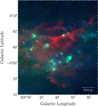
Figure 1. An overview of the Sgr E region. The red shows the 870 μm 12CO (J = 3–2) emission integrated over the entire line-of-sight velocity range of ±300 km s−1 (CHIMPS2; Eden et al. 2020), the green shows 70 μm (Herschel Hi-GAL; Molinari et al. 2010), and the blue shows 8 μm (Spitzer GLIMPSE; Benjamin et al. 2003). The white circle is the field of view of the ALMA observation.
Download figure:
Standard image High-resolution image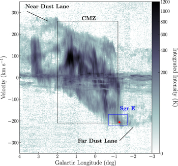
Figure 2. An overview of the inner Galaxy in l–v space, as seen in the 12CO (J = 3–2) emission (CHIMPS2; Eden et al. 2020). The black box indicates the longitude range of the CMZ (l = 2° to −11). The blue box represents the line-of-sight velocity range (−170 km s−1 > vLOS > −220 km s−1) and the longitude range (−07 > l > −17) of the Sgr E region. The red circle represents the (l,v) coordinate of the H ii region, which our data is centered on.
Download figure:
Standard image High-resolution imageThe radio continuum emission from these regions has been observed and reported on in the literature over the last few decades (Liszt 1992; Gray et al. 1993; Cram et al. 1996; Anderson et al. 2020), revealing the peculiar characteristics of Sgr E when compared to other Galactic H ii region complexes. Unlike the H ii regions in other star-forming complexes, the Sgr E H ii regions are similar in size and lack a central concentration, with most sources having diameters of 1–4 pc and a median separation of ∼20 pc between them (Anderson et al. 2020). The complex is also associated with a 3 × 10⁵ M⊙ molecular cloud that exhibits a strong velocity gradient (−170 km s−1 to −220 km s−1) from east to west along the Galactic plane (Anderson et al. 2020).
With a stellar population that is thought to contain mostly B2- to O8-type stars, Sgr E has an estimated age of 3–5 Myr (Gray et al. 1993; Anderson et al. 2020). Recent simulations suggest that stars currently contained in the Sgr E complex formed in the far dust lane a few Myr ago, and that they will eventually overshoot the CMZ and collide with the near dust lane (Anderson et al. 2020).
Observations of the Sgr E complex present a unique opportunity to study a highly dynamic region, with properties that are distinct from other star-forming regions observed in both the CMZ and the Galactic disk. It is anomalous, as it is the only star-forming region located at the intersection between the dust lanes and the CMZ. Additionally, the large velocity gradient across the Sgr E region implies that the gas is subject to very strong accelerations. Despite its unusual properties, there are only a handful of papers that focus on the Sgr E complex. It is therefore important to study the Sgr E region in greater detail, to gain insights into the properties of the interstellar medium and the process of star formation in highly dynamic environments.
In this paper, we present the first high-resolution Atacama Large Millimeter/submillimeter Array (ALMA) observations in several CO (1-0) emission lines toward a known Sgr E H ii region, previously identified in Anderson et al. (2020) and located at l = 358720 and b = 0011, a projected distance of 175 pc from the Galactic center. The H ii region has a measured central velocity of −206.1 km s−1 and a diameter of 2.7 pc. Our paper is organized as follows. In Section 2, we provide details of the ALMA observations and our final data products. In Section 3, we present CO spectral line observations of filaments in the Sgr E region and report on their physical and kinematic structures. In Section 4, we contextualize the unique properties of these filaments within the broader context of large-scale Galaxy dynamics. Finally, Section 5 presents a brief summary of our conclusions.
2. Observations
2.1. ALMA Data
The data that we present in this paper are part of a larger survey that was observed using ALMA in Cycle 7 (Project code 2019.1.01240.S; PI: E.A.C. Mills). The observations were completed over eight sessions, with an average of 45 antennas, between 2019 October 31 and November 24. This survey consisted of 25 pointings within the central 50 of the Galaxy. In this paper, we present results from a single pointing with a field of view (half-power beamwidth) of 52'' (2 pc) toward the Sgr E complex, centered at l = 358720 and b = 0011 (α = 17h42m29.90s, δ = −30° 1'14 0). The observations were made in the C43-2 configuration, with baselines ranging between 15 and 697 m.
Our observations were made at a single frequency setting at 3 mm (ALMA Band 3) over a total of eight spectral windows. Five of these had bandwidths of 234.38 MHz (∼640 km s−1), 9 centered on spectral lines, while the remaining three had bandwidths of 1875 MHz, covering continuum emission. The continuum spectral windows were centered on the frequencies 97.980953 GHz, 100.900000 GHz, and 102.800000 GHz. The remaining spectral windows were centered on the spectral lines 12C16O (1-0) (hereafter, 12CO), 12C17O (1-0) (hereafter, C17O), 13C16O (1-0) (hereafter, 13CO), 12C18O (1-0) (hereafter, C18O), and H(40)α.
We focus our analysis on the 12CO, 13CO, and C18O lines. The properties for these spectral line data cubes are given in Table 1. The calibration of the data was performed in the Common Astronomy Software Applications package (CASA: versions 5.6.1–8), using the ALMA pipeline (McMullin et al. 2007). The imaging of the continuum, as well as the 12CO, 13CO, and C18O lines, was performed in CASA, using the tclean task, with a robust weighting of 1.0, so that the observations were sensitive to a combination of both point source emission and extended emission.
Table 1. Properties of the CO Spectral Line Data Cubes
| Spectral Line | Rest Frequency | Beam Position Angle | Beam Size | LAS a | rms | |||
|---|---|---|---|---|---|---|---|---|
| (GHz) | (deg) | (arcsec) | (pc) | (arcsec) | (pc) | (mK) | (mJy beam−1) | |
| 12C16O (1-0) | 115.271202 | −21.3 | 24 × 14 | 0.09 × 0.06 | 212 | 0.84 | 395 | 13.3 |
| 13C16O (1-0) | 110.201354 | −28.6 | 24 × 17 | 0.09 × 0.07 | 224 | 0.89 | 297 | 11.6 |
| 12C18O (1-0) | 109.782176 | −28.6 | 24 × 17 | 0.09 × 0.07 | 226 | 0.90 | 278 | 10.7 |
Note.
a The largest angular scale, given by , where
  is the length of the shortest baseline (https://almascience.nrao.edu/about-alma/alma-basics).
Download table as: ASCIITypeset image
The rest frequency, beam size, beam position angle, and per-channel rms noise for each CO data cube are given in Table 1. The final 12CO images have 028 pixels (0.011 pc), and the final 13CO and C18O images have 034 pixels (0.013 pc). The velocity resolution of the spectral line data is approximately ∼0.3 km s−1 (∼0.11 MHz). All images are sensitive to size scales up to 21'' (∼0.84 pc; see the largest angular scale, or LAS, in Table 1).
Before any analyses were performed, we used the reproject and spectral_interpolate functions from the Spectral Cube package (Ginsburg et al. 2019) to regrid each data cube to match the C18O data cube. The resulting cubes have the same voxel 10 sizes, with 0.013 pc pixels and 0.33 km s−1 velocity channel widths. For the creation of the line ratio maps, we additionally smoothed the cubes to a common beam size taken from the C18O data cube.
2.2. Ancillary Data
In Sections 1 and 4, we use 12CO (J = 3–2) spectral line data from the CO Heterodyne Inner Milky Way Plane Survey 2 (CHIMPS2; Eden et al. 2020) to generate longitude–velocity (l–v) diagrams of the inner Galaxy. The CHIMPS2 observations were completed using the James Clerk Maxwell Telescope and have an angular resolution of 15'' and a velocity resolution of 1 km s−1.
3. Results and Analysis
We investigate the spatial and kinematic properties of the molecular gas in the 12CO, 13CO, and C18O spectral line cubes. The bulk of our analysis is performed with the 13CO and C18O data cubes, where we use the brighter 13CO line emission for filament identification, and the less optically thick C18O line emission for measuring the physical properties of each filament. We discuss the relative optical depths for each data cube in Section 3.3. Full-resolution channel map images from the 12CO and C18O data cubes are included in Appendix A.
3.1. Overview of Filamentary Structure
We report on a collection of filaments observed in the CO emission toward our Sgr E pointing. Our findings indicate the existence of numerous linear filamentary structures that are oriented parallel to the Galactic plane. In this paper, we focus our in-depth analysis on two of the filaments identified (see Section 3.1.1).
To provide a brief overview of these filaments, we present five integrated intensity maps from the 13CO data cube, with the emission summed over 5 km s−1 velocity ranges (Figure 3). These span an overall velocity range of −200 km s−1 to −225 km s−1. Molecular gas filaments are clearly observed in panels (a), (d), and (e) of Figure 3. The orange and blue contours in Figure 3 indicate the emission associated with two of the most prominent filaments identified in our data, which we later refer to as "filament 1" and "filament 2," respectively. We expand on these filament regions in more detail in Section 3.2.
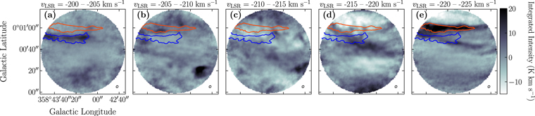
Figure 3. Integrated intensity (moment 0) maps from the 13CO data cube. Each image shows the integrated intensity over a range of 5 km s−1. The specific velocity ranges are indicated above each image. The top—orange—contour indicates the region that we define for filament 1, while the bottom—blue—contour indicates the filament 2 region. The beam is indicated in the lower right corner of each channel map.
Download figure:
Standard image High-resolution imageIn panel (a) of Figure 3, we identify a single filament, and in Figure 3(e), we identify two filaments. All three filaments are very straight and are oriented nearly parallel to the Galactic plane (see Section 3.2.1 for more details of the physical characteristics of the filaments). We note that the two filaments observed in Figure 3(e) are separated by ∼0.1 pc. The brightest filament in Figure 3(e), located at b = 00° 01'00'', has a position angle of approximately ∼2° with respect to the Galactic plane, whereas the less bright filament has a more pronounced angle of ∼15°. The less bright filament appears to be cospatial with the linear structure observed in Figure 3(d), which might indicate that the emissions observed in both velocity ranges are part of the same filamentary structure.
3.1.1. Filament Identification
We focus our subsequent analysis on the quantitative properties of a subset of the observed filamentary structures. This subset contains two filaments, which we label "filament 1" and "filament 2." Both of these filament regions are shown in Figure 3 as orange (filament 1) and blue (filament 2) contours. These regions were chosen based on the criterion that they were both observed in the emission for the three brightest CO isotopologues. Additionally, filaments 1 and 2 are well separated from each other, by at least 0.1 pc in position–position space, and by more than 10 km s−1 in velocity space.
The emission located in the filament 1 region is mostly observed between vLSR = −220 km s−1 and −225 km s−1 (see Figure 3(e)). Conversely, in the filament 2 region, the brightest emission is observed between vLSR −200 km s−1 and −205 km s−1 (see Figure 3(a)). Another emission feature is seen in panels (d) and (e) of Figure 3. We omit this feature from our analysis, since it is not well separated from the other two filament regions and is not visible in the C18O data. From these integrated intensity maps, we see that filament 1 is located at the Galactic latitude b = 00°01'00'' and filament 2 is located at b ∼ 00°00'50''.
We identified these filament regions using full-resolution velocity channel maps from the 13CO data cube. As seen in Figure 4, these channel maps have a channel width of 0.3 km s−1 and are centered on the velocity ranges containing the filaments of particular interest. We used the −223 km s−1 and −203 km s−1 channels of the 13CO data cube to identify filament 1 and filament 2, respectively (see Figure 4). These two channels were used for quantitative analysis, since the emission related to the filaments was brightest at these velocities. We used the 13CO data for filament identification, since it exhibits a higher signal-to-noise ratio (S/N) compared to the C18O data.
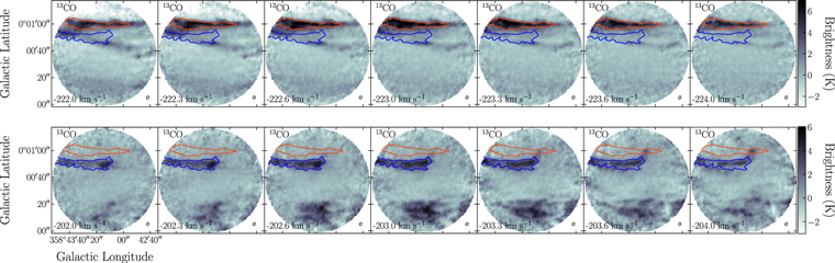
Figure 4. The full-resolution velocity channel maps for the spectral line 13CO used to identify filaments 1 and 2, with channel widths of ∼0.3 km s−1. The channel maps on the top row span the velocity range of −222.0 km s−1 to −224.0 km s−1. The channel maps on the bottom row span the velocity range of −202.0 km s−1 to −204.0 km s−1. In each image, the top—orange—contour indicates the region that we define for filament 1, while the bottom—blue—contour indicates the filament 2 region. The beam is indicated in the lower right corner of each channel map.
Download figure:
Standard image High-resolution imageTo define the filament regions, we created Boolean masks from the aforementioned channel map images, using brightness thresholds of 4.0 K for the 13CO −223 km s−1 channel and 2.0 K for the 13CO −203 km s−1 channel. These thresholds were chosen by eye, with the aim of ensuring that the boundaries of the filament regions contained the bulk of the filament emission. To completely isolate each filament, we manually masked out bright regions that were separated from the filament by more than 0.1 pc, a separation slightly larger than the semimajor axis of our beam (∼0.09 pc).
For velocities spanning −222 km and −224 km s−1, the relative shape and brightness of filament 1 varies minimally (Figure 4). We note that the filament below it passes through the filament 2 region at an angle. We also highlight the emission from the filament 2 region in Figure 4, for velocities spanning −202 km to −204 km s−1. We note that filament 2 is spatially isolated from other emission structures in the field of view.
3.1.2. Moment Analysis
To further explore the general physical and kinematic properties of the filaments, we performed moment analyses for each spectral line cube in the velocity range of −197 km to −231 km s−1 (see Figures 5 and 6). We present these results with the understanding that although moment analyses provide a standard way of parameterizing the spatial and kinematic properties of the gas observed in three-dimensional data cubes, it does have limitations with regard to interpretation, as it condenses three dimensions of information into a two-dimensional representation and can obfuscate complex spectral line structures (Henshaw et al. 2016).
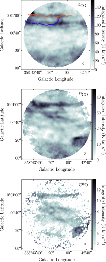
Figure 5. Spatially masked moment 0 maps generated from data in the velocity range of −197 km s−1 to −231 km s−1 for 12CO (top), 13CO (middle), and C18O (bottom). In the 12CO image, the orange line represents the filament 1 p–v slice path, while the blue line represents the filament 2 p–v slice path. For each image, the beam is indicated in the lower right corner.
Download figure:
Standard image High-resolution image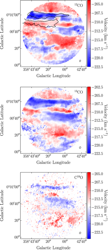
Figure 6. Spatially masked moment 1 maps generated from data subcubes in the velocity range of −197 km s−1 to −231 km s−1 for 12CO, 13CO, and C18O, respectively. In the 12CO image, the black contours indicate the filament 1 and filament 2 regions. For each image, the beam is indicated in the lower right corner.
Download figure:
Standard image High-resolution imageBefore performing any moment calculations, we masked each data cube to remove the low-S/N regions in our images. We first generated a two-dimensional mask that only included pixels with a maximum intensity along the spectral axis that was three times greater than the standard deviation noise level determined from a line-free region of the spectrum at each pixel. Additionally, we applied a three-dimensional mask to each data set that excluded regions where the signal was less than the 1σ noise level.
With both masks applied to the corresponding data set, we proceeded to calculate the zeroth-order and first-order moment maps for each isotopologue. These calculations were performed using the Astropy SpectralCube (Ginsburg et al. 2019) Python package. This package performs moment analysis using the standard methods, which we briefly describe in this section.
We calculated the zeroth-order moment for each isotopologue by integrating the intensity along the spectral axis of the data cube at each pixel. Moment 0 maps for all three spectral lines are shown in Figure 5. We see that in the Galactic latitude range spanning b = 0°00'40''–0°01'00'', there are linear filamentary molecular gas structures that appear to align closely with the orientation of the Galactic plane. Although these filaments appear to exist in the same regions for each isotopologue, it can be seen that the spatial extent of the structures seen in the 13CO and C18O emission are visually more similar to each other than to the structures seen in the 12CO emission. This is likely due to the 12CO spectral line having a higher optical depth, a property that we discuss in more detail in Section 3.3. We see from the 13CO and C18O data that the filament 1 region (located at b ∼ 0°01'00'') seems to contain the largest amount of emission in this velocity range, although this is less apparent when we look at the 12CO moment 0 map. The emission from the filament 2 region (located around b ∼ 0°00'50'') is overall less bright than that from the filament 1 region.
We further calculated the intensity-weighted velocity of the spectral line, also known as the first-order moment. These moment 1 maps are shown in Figure 6, where we see that most of the material located in filament 1 is observed at velocities between −220 and −223 km s−1. On the other hand, most of the emission observed in the filament 2 region spans velocities between −202 and −205 km s−1. These trends are observed in all three moment 1 maps.
3.2. Filament Properties
The next phase of analysis focuses on quantifying the specific physical and kinematic characteristics of filaments 1 and 2. In Section 3.2.1, we present radial brightness temperature profiles of each filament, created using the RadFil package, and estimate their length, width, and orientation with respect to the Galactic plane. In Section 3.2.2, we investigate the velocity structure of each filament. We take position–velocity (p–v) slices along both filaments and identify four distinct velocity components. In addition to this, we create velocity profiles for each component in p–v space using RadFil. We then estimate the velocity gradients and FWHM widths from these results. To round out our investigation of the kinematic properties, we also present averaged spectra for all three spectral lines taken from the filamentary region.
For our analysis, we consider how the optical depth in our data might affect the accurate determination of filament properties. In the Galactic center, the spectral line ratio 12CO/13CO ∼20, while the ratio 12CO/C18O ∼250 (Wilson & Rood 1994). Since the C18O (1-0) emission is the least abundant among the three isotopologues, it is the least likely to be optically thick. In light of this, we use the C18O data to generate our brightness temperature profiles and our velocity profiles, in an effort to make estimates that are as accurate as possible. We discuss the effects of optical depth on our calculations in greater detail in Section 3.3.
3.2.1. Physical Characteristics
We investigated the physical properties of the Sgr E filaments primarily with the use of the Python packages RadFil (Zucker & Chen 2018) 11 and FilFinder (Koch & Rosolowsky 2015). 12 We did this by applying a Boolean mask of the filament 1 and filament 2 regions (see Section 3.1.1) onto the −223 km s−1 and −203 km s−1 C18O channel images, respectively (Figure 17 in Appendix A). We then created a 1 pixel wide filament spine for each filament in the masked images, through the use of RadFil, which calls upon the FilFinder package. FilFinder produces this spine object by performing medial axis skeletonization on the filament region, a process that finds a set of all pixels within the given mask that has more than one closest point on the shape's boundary. This means that each pixel contained within the spine object is at the maximum distance that it can be from the edge of the filamentary region. A more detailed explanation of the medial axis skeletonization—or medial axis transformation—process can be found in Koch & Rosolowsky (2015).
Once the spines were produced, we used RadFil to calculate the length of each filament (see Table 2). From here, we calculated a linear fit from the spine object in pixel coordinates, using np.polyfit. We then used this line to estimate the angle of the filament from the Galactic plane in degrees, which we report in Table 2.
Table 2. Physical Properties for Filaments 1 and 2
| Filament | Spine Length (pc) | FWHM Width (pc) | Aspect Ratio | Position Angle (°) a |
|---|---|---|---|---|
| 1 | 2.2 | 0.12 ± 0.02 | 4.5:1 | 1.8 |
| 2 | 1.9 | 0.11 ± 0.01 | 5.4:1 | 1.2 |
Note.
a The absolute two-dimensional projected position angle between the filament and the Galactic midplane.Download table as: ASCIITypeset image
We then used RadFil to produce brightness temperature profiles for both filaments, shown in Figure 7. To do this, RadFil smooths the filament spine and takes evenly sampled cuts, for which brightness temperature profiles perpendicular to the spine are calculated at each site along the filament. A thorough description of this process is given in Zucker & Chen (2018). We used a sampling interval of 1 pixel along the spine (∼0.01 pc). We created the filament 1 brightness temperature profile from the C18O −223 km s−1 channel image and the filament 2 profile from the C18O −203 km s−1 channel image. As seen in Figure 7, we generated Gaussian fits from the brightness temperature profiles for each filament using RadFil. For both filaments, we used a fitting distance of 0.05 pc from the center of the filament, where the fitting distance is the region for which the Gaussian fit is calculated. We then estimated the filament widths in parsecs, using the FWHM values of the Gaussian fits, which are recorded in Table 2. To calculate the filament aspect ratios, we assumed a cylindrical geometry for the filaments and set the cross-sectional area of the cylinder equal to the area under the Gaussian fits for each filament (Figure 7). From there, we divided the filament length by the estimated effective filament diameter, to acquire the filament aspect ratios.
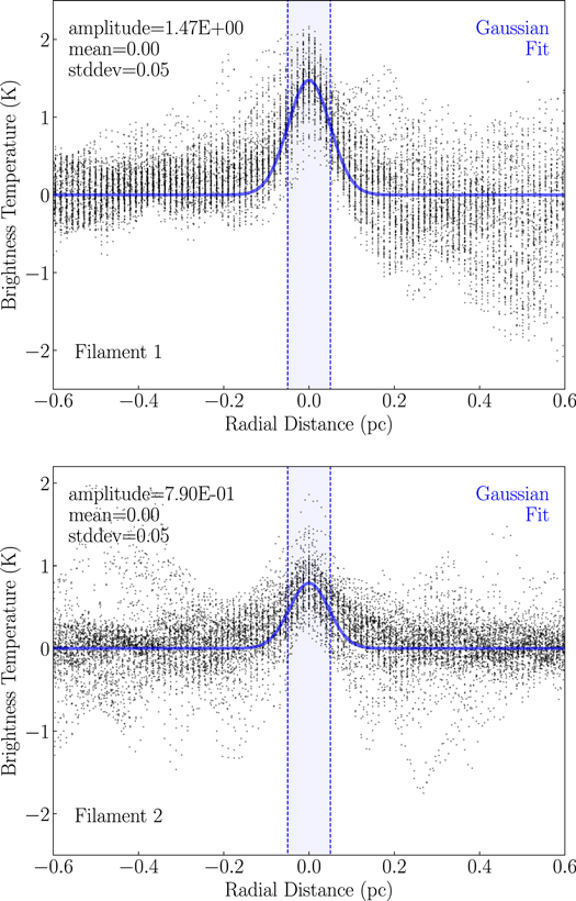
Figure 7. Top: the brightness temperature profile for filament 1, taken from the −223.0 km s−1 C18O channel image. Bottom: the brightness temperature profile for filament 2, taken from the −203 km s−1 C18O channel image. The blue lines plotted in both figures are the Gaussian fits for each filament profile, made using a fitting distance of 0.05 pc from the center of the filament. The radial distance is the distance from the center of the filament.
Download figure:
Standard image High-resolution imageFrom these results, we see that both filament 1 and 2 exhibit similar physical dimensions, as both have lengths of ∼2 pc, FWHM widths of ∼0.1 pc, and aspect ratios of ∼5:1. We stress that these are lower-limit calculations for the filament lengths and aspect ratios, as the filaments appear to extend out of the field of view. We also note that filament widths of 0.1 pc, similar to our spatial resolution, suggest that these may be unresolved and could be narrower. Both filaments are well aligned with the Galactic plane, with modest position angles of 1.8 (filament 1) and 12 (filament 2), and they are oriented so that the material at lower Galactic longitudes is closer to the Galactic plane.
3.2.2. Velocity Structure of Filaments
We take p–v slices along filaments 1 and 2 for all three data cubes in the range of −197 km s−1 to −231 km s−1, through the use of the pvextractor package (Ginsburg et al. 2016a). The p–v slices were made along the filament spines calculated using RadFil. By convention, the path begins (offset = 0 pc) at higher Galactic longitudes and moves to lower longitudes (from left to right in the figures). The paths for the p − v slices are shown in Figures 5 and 6 as the orange (filament 1) and blue (filament 2) lines. We calculated the p–v slices with a given width of 2'' (∼0.09 pc), about the same size as the semimajor axis of our beam.
Although the purpose of the RadFil package is to calculate radial profiles in position–position space, as we described in Section 3.2.1, we also used it in p–v space for this project, to determine certain kinematic properties of the filaments, namely their velocity gradients and velocity widths. We again used the FilFinder package to create a "spine" for the brightest region calculated along the aforementioned p–v slice. Just as before, we generated a linear fit of the spine for each notable velocity component. We then calculated the velocity gradient of the filament by determining the slope of the resulting best-fit line. We use the median value of the pixel coordinates of the best-fit line to estimate the central velocity for each component.
In the p–v diagram sliced along filament 1 (Figure 8), we observe two distinct velocity components that are seen in all three CO isotopologues. We label these regions as velocity components "1A" and "1B." These components are separated by ∼14 km s−1 along the length of the filament. We take velocity component 1A to be the component that is associated with filament 1, as it is centered around −223 km s−1 and is the brightest of the two in each diagram, especially with regard to the 13CO and C18O emissions. In comparison, the 1B component, centered at −209 km s−1, is less bright and has a narrower velocity width than the 1A component. From inspections of the data cubes, we believe that velocity component 1B is associated with local nonfilamentary CO emission. For 12CO and 13CO in Figure 8, there is a "bridge" of emission located at an offset of ∼1.0 pc, a feature that could indicate an interaction between filament 1 and the gas associated with velocity component 1B. We note that components 1A and 1B are both present along the full length of the filament, and have velocity gradients of 0.35 km s−1pc−1 and 0.57 km s−1 pc−1, respectively.
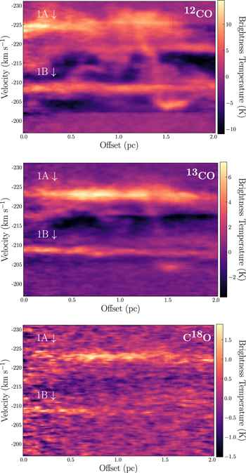
Figure 8. The filament 1 p–v diagrams for 12CO (top), 13CO (middle), and C18O (bottom), respectively. The p − v slice starts at the end of the filament that is closer to the Galactic center, so the offset represents the distance along the p − v slice as we move from left to right along the filament 1 spine (see Figure 5).
Download figure:
Standard image High-resolution imageSimilarly, we see in Figure 9 that there are two prominent velocity components along filament 2, which we label "2A" and "2B." In the 13CO and C18O p–v diagrams, we see that components 2A and 2B have central velocities of −219 km s−1 and −203 km s−1, respectively. These velocity components are separated by ∼16 km s−1 along the length of filament 2. Velocity component 2A has a measured velocity gradient of 5.2 km s−1 pc−1, while component 2B exhibits a small velocity gradient of 0.0017 km s−1 pc−1. In the 12CO and 13CO figures, it is clear that component 2B is much brighter than component 2A, but this is more ambiguous in the C18O data, which only have a faint signal for both components. Based on its central velocity of −203 km s−1, we believe that velocity component 2B is definitely associated with filament 2. The central velocity and velocity gradient of velocity component 2A lead us to interpret it as emission that is associated with the other filament-like feature observed in panels (d) and (e) of Figure 3.

Figure 9. The filament 2 p–v diagrams for 12CO (top), 13CO (middle), and C18O (bottom), respectively. The p − v slice starts at the end of the filament that is closer to the Galactic center, so the offset represents the distance along the p − v slice as we move from left to right along the filament 2 spine (see Figure 5).
Download figure:
Standard image High-resolution imageFor the velocity components 1A, 1B, and 2B, the velocity of the gas seems to decrease slowly as we move toward lower Galactic longitudes, away from the Galactic center, behavior that is consistent with the large-scale trend along the far dust lane. In Figure 9, it is important to note the apparent absorption at −220 km s−1 in the 12CO p–v diagram. This is a feature that is not present in the p–v diagrams for 13CO and C18O, and it may be the result of the 12CO emission being optically thick toward this region.
In a process analogous to the creation of the brightness temperature profile, we calculated velocity profiles along each velocity component that we identified. We generated Gaussian fits to the velocity profiles and recorded the FWHM line widths. All of these analysis steps were performed for each velocity component using the C18O p–v diagrams (Figures 8 and 9). We used the higher-S/N 13CO p–v data to mask the C18O data. We used masking thresholds of 2.8 K, 1.8 K, 1.0 K, and 2.1 K for velocity components 1A, 1B, 2A, and 2B, respectively.
The velocity profiles with Gaussian fits for each component are given in Figure 10, and the FWHM velocity line widths (velocity dispersions) calculated from these fits are reported in Table 3. We see that both filament 1 and 2 (velocity components 1A and 2B) have velocity line widths of 2.0 km s−1. Filament 1 and 2 both have velocity gradients <1 km s−1 pc−1, with filament 2 having a very small velocity gradient of 0.0017 km s−1 pc−1. The larger velocity gradient and line width observed in component 2A might be further evidence that it is not associated with gas located along the elongated axis of a coherent filament.

Figure 10. Velocity profiles generated from the C18O p − v diagrams (see Figures 8 and 9). Top left: the profile for velocity component 1A, centered at approximately −223 km s−1. Top right: the profile for velocity component 1B, centered at approximately −208 km s−1. Bottom left: the velocity profile for velocity component 2A, centered at approximately −220 km s−1. Bottom right: the profile for velocity component 2B, centered at approximately −203 km s−1. The blue lines in each figure are the Gaussian fits for each velocity profile, made using a fitting distance of 1.3 km s−1 from the central velocity. The FWHM velocity line widths for each velocity component are reported in Table 3.
Download figure:
Standard image High-resolution imageTable 3. Kinematic Properties for the Velocity Components Identified within Each Filament Region
| Velocity Component | Central Velocity | Velocity Gradient | FWHM Line Width |
|---|---|---|---|
| (km s−1) | (km s−1 pc−1) | (km s−1) | |
| 1A a | −223 | 0.35 | 2.0 ± 0.28 |
| 1B | −209 | 0.57 | 1.3 ± 0.13 |
| 2A | −219 | 5.2 | 2.4 ± 0.46 |
| 2B b | −203 | 0.0017 | 2.0 ± 0.19 |
Notes.
a The velocity component associated with filament 1. b The velocity component associated with filament 2.Download table as: ASCIITypeset image
To further investigate the velocity structures of each filament, we extract spectra at four separate locations along the filaments for all three isotopologues (Figure 11). We chose two sufficiently bright locations on either side of each filament to better represent its full length. In order to improve the S/N, we averaged the spectra in a circular aperture with a diameter three times the semimajor axis of the beam. These apertures are indicated in cyan in Figure 12.
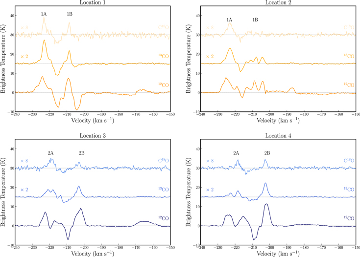
Figure 11. Spectra for 12CO, 13CO, and C18O taken from four different regions and averaged over a circular aperture with a diameter that is three times larger than the semimajor axis of the beam. Regions 1 and 2 are pulled from two different locations along filament 1, whereas regions 3 and 4 are located along filament 2. The spectra for 13CO and C18O are scaled by factors of 2 and 8 and offset by 15 K and 30 K, respectively, so that they can be seen clearly. Spectral peaks are labeled with their corresponding velocity components identified in the p–v diagrams (Figures 8 and 9).
Download figure:
Standard image High-resolution image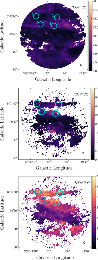
Figure 12. Ratio maps for 12C16O/13C16O (top), 12C16O/12C18O (middle), and 13C16O/C18O (bottom). These ratio maps were calculated from the moment 0 maps seen in Figure 5, with some additional masking (see Section 3.3). The circles outlined in cyan indicate the regions that the spectra were averaged over. In the top image, the regions are labeled with the numbers assigned to the spectra in Figure 11.
Download figure:
Standard image High-resolution imageThe spectra taken at locations 1 and 2 are given in orange and correspond to the filament 1 region, whereas locations 3 and 4 are given in blue and correspond to the filament 2 region. We denote the spectral peaks using the velocity component labels defined in Section 3.2.2. Overall, we see that the labeled peaks are observed in the data for all three spectral lines. We note that the 12CO spectrum at location 2 has a peak at approximately −225 km s−1, which is displaced from the peak at −223 km s−1 observed in the 13CO and C18O spectra. Similarly, a spectral line component is observed at −220 km s−1 in the 13CO and C18O spectra, at location 4, which is noticeably absent from the 12CO spectrum. We also note that there are regions of "negative" brightness, which appear next to the spectral emission lines, that are observed at every location. These are especially exaggerated in the 12CO emission, but do occur in the 13CO and C18O emissions as well. These can be interpreted either as regions of self-absorption on a more diffuse CO field or as an interferometric effect created during the image cleaning process.
3.3. Effects of Opacity
It is well known that the spectral lines 12CO (1-0) and 13CO (1-0) can be optically thick in observations made toward the Galactic Center, where there is a very large amount of molecular gas. In the context of our data set, observations of spectral lines with high opacity may result in the artificial line width broadening the filaments in our field of view. However, since one of our key results is that our line widths are narrower than expected, this would only serve to make our findings more intriguing.
To investigate the effects of opacity on our data set, we computed line ratio maps (Figure 12) for 12C16O/13C16O, 12C16O/12C18O, and 13C16O/12C18O, from the integrated intensity maps (Figure 5). We interpret these ratios as being indicative of changes in the optical depth across the field. Since the LAS is expected to vary by at most 6% between the 12CO images and the 13CO and C18O images, and the structure seen in the 13CO and C18O images does not reach the size scale of the LAS, the effects of interferometric filtering should be negligible, and the interpretation that these ratios reflect changes in the optical depth is reasonable.
To ensure that the same number of pixels were being integrated over for each data cube, we updated the masking so that both moment 0 maps in each ratio calculation were masked identically. To do this, we generated masks for each isotopologue individually, as we did for the integrated intensity maps (see Section 3.1.2). We then applied the mask from the other data set being used in the ratio calculation to the first data set. For example, in the 12CO/13CO line ratio calculation, we masked the 12CO data cube and the 13CO data cube with a combination of both the 12CO and 13CO masks that we generated previously. Once all the data cubes were masked appropriately, we generated the moment 0 images and directly divided them to produce the desired line ratio maps.
Near the Galactic center, the expected abundance ratio for 12C/13C ≈ 20 (Wilson & Rood 1994; Humire et al. 2020), whereas the ratio for 16O/18O ≈ 250 (Wilson & Rood 1994). Given the high column densities and optical depths of our images, we expect that most of the carbon along the line of sight is in CO and that these isotope ratios are analogous to the corresponding CO isotopologue ratios.
In our 12CO/13CO line ratio map, we see that most of the field of view exhibits a line ratio less than 10, indicating that 12CO is optically thick. The filament 1 region exhibits a 12CO/13CO line ratio <5, which suggests that 13CO is also optically thick in this region.
Similarly, the line ratios seen in the C16O/C18O ratio map are far lower than the canonical ∼250 value. Considering the high opacity of each spectral line, we decided to use the C18O data to calculate the filament widths, velocity widths, and velocity gradients, since it is likely the most optically thin line that we observed.
It should be noted that observations were also made for the C17O (1-0) spectral line, which is even less abundant than the C18O isotopologue (e.g., Wilson & Rood 1994). Although there is some faint C17O emission located at Galactic latitudes south of the observed filaments, there is no clear emission in the filament regions that we define. As a result, we cannot provide evidence of optical depth effects on our results using the C17O data set.
3.4. Dust Continuum Emission
In Figure 13, we see that filaments 1 and 2 show no morphological association with the 3 mm dust continuum observed at the same pointing. We assume that this continuum emission is primarily from the H ii region located at this pointing. The central line-of-sight velocity of the H ii region is −206.1 km s−1 (Anderson et al. 2020), compared with central velocities for filaments 1 and 2 of −223 km s−1 and −203 km s−1, respectively. Therefore, though the filaments show no clear morphological association with the continuum emission, they are consistent with being in relatively close proximity in p–p–v space, particularly filament 2.
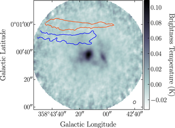
Figure 13. Continuum emission (3 mm) located toward our pointing of the Sgr E region. The top—orange—contour indicates the filament 1 region, while the bottom—blue—contour indicates the filament 2 region. The beam is indicated in the lower right corner of the figure.
Download figure:
Standard image High-resolution image4. Discussion
Our analysis has characterized two prominent filamentary structures toward the Sgr E region and provided information regarding their physical and kinematic properties. We find these filaments to have a linear structure, with small angles toward the Galactic plane.
In this section, we intend to contextualize the unique features of these structures with respect to the large-scale gas dynamics occurring toward the Sgr E region. To do this, we compare the physical properties of the Sgr E filaments with properties observed in molecular clouds and filaments in the CMZ, as well as the Galactic disk. We then discuss the known properties of the H ii region associated with our field of view. After this, we provide a discussion of the physical mechanisms that might be creating these filaments. We close this section by discussing some open questions that these data present and some predictions to be tested in the future.
4.1. Comparison of Sgr E Properties with the CMZ and the Galactic Disk
The Sgr E region is located at the intersection between the far dust lane and the CMZ. The H ii regions associated with the Sgr E complex have some of the highest absolute line-of-sight velocities (∼−200 km s−1) of any known star-forming regions in the CMZ or the Galactic disk (Anderson et al. 2014).
In Figure 14, we provide an l–v diagram from the CHIMPS2 12CO (3-2) survey, where the orange and blue contours represent the 13CO emission associated with filaments 1 and 2 at a temperature threshold of 0.0075 K. We see that the emission associated with the velocity components 1B and 2B is coincident with the overall large-scale distribution of the CHIMPS2 12CO data (Figure 14). On the other hand, the emission associated with velocity components 1A and 2A appears to be offset from the main distribution of gas, toward more negative velocities, by ∼5 km s−1. To check if any emission at this velocity was detected near the filament regions in the CHIMPS2 data cube, we created an integrated intensity map for velocities ranging from −220 km s−1 to −225 km s−1. We find that a 12CO (3-2) emission is located in the region of our filaments for this velocity range, but it is faint compared to the nearby emission. We conclude that this emission at ∼−223 km s−1 is not apparent in Figure 14, because it is much fainter than the nearby emission, especially when integrated over Galactic latitude.
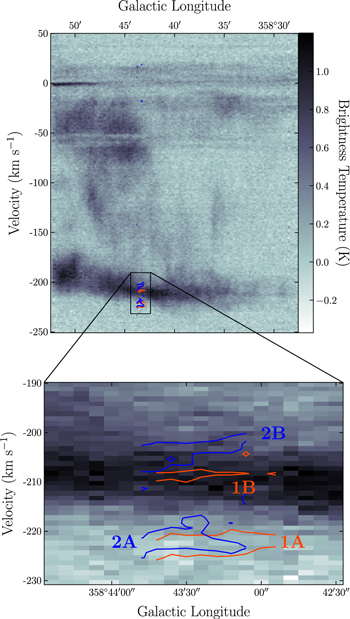
Figure 14.
l–v diagram of the 12CO (J = 3 − 2) emission (CHIMPS2; Eden et al. 2020) toward the Sgr E region, integrated over the range  < 0175. The data have a spatial resolution of 15'' and a velocity resolution of 1 km s−1. The black rectangle represents the boundary of the zoomed-in region shown at the bottom of the figure. The zoomed-in region spans the velocities −190 km s−1 to −230 km s−1. The red contours indicate the emission from the Sgr E 13CO data cube in the same l–v region at a temperature threshold of 0.0075 K.
Download figure:
Standard image High-resolution imageThe lengths and radial widths of our filaments are well within the expected range for the physical dimensions of filaments in the Galaxy (Hacar et al. 2022). There is discussion within the literature about the presence of a mean universal filament width of FWHM ∼ 0.1 pc. However, there is evidence that measured filament widths may depend on the filament scale and density (Hacar et al. 2022, and see references therein), as well as on the resolution of the observations (Panopoulou et al. 2022). As a result, we conclude that it is likely coincidental that our filaments have an FWHM ∼ 0.1 pc, and that this measurement does not suggest the existence of a universal filament width.
The FWHM line widths of the filament velocity components reported in Table 3 range between 1.3 and 2.4 km s−1. When we convert these line widths into a total gas velocity dispersion,
13
σtot, and divide this by the typical sound speed for CO bright molecular gas (cs
= 0.2 km s−1), we find that the velocity dispersions of our filaments, in units of sound speed, are between  = 2.3–3.9. These values are well within the range that is observed for other Galactic filaments with lengths of ∼2 pc, approximately
  = 1–10 (Hacar et al. 2022).
The velocity dispersions of the molecular gas structures in the CMZ tend to be much larger than those observed in the disk (Shetty et al. 2012; Henshaw et al. 2016). At a similar subparsec size scale, our FWHM line widths are narrower than those measured in dense star-forming cores in the CMZ, with velocity dispersions from 1 to 4 km s−1, corresponding to FWHM line widths of ∼2–9 km s−1 (D. Callanan et al. 2022, in preparation).
Interestingly, the velocity line widths observed in our filaments seem to be similar to those of filaments in the Galactic disk, and somewhat narrow when compared to gas in the CMZ. The larger line widths for gas in the CMZ are thought to be driven mostly by turbulence (Shetty et al. 2012; Kauffmann et al. 2017), which may be caused in part by collisions from gas streaming into the CMZ from the dust lanes (Henshaw et al. 2022). Based on our observations, the gas in the Sgr E region appears to be relatively quiescent when compared to gas within the CMZ, as it travels along the far dust lane.
4.2. Discussion of the Origin of Sgr E's Filamentary Structure
Using high-resolution CO spectral line data, we have shown that the Sgr E region contains multiple filaments that exhibit a linear structure with an orientation that is nearly parallel to the Galactic plane. These filaments also possess an interesting kinematic structure, with velocity components along the line of sight that have comparatively narrow velocity line width values.
We propose that the properties of the Sgr E filaments may be due to their unique placement between the CMZ and the far dust lane. As previously mentioned, the molecular gas in the Sgr E region is located where the far dust lane meets the CMZ, and moves with a high line-of-sight velocity of ∼−200 km s−1. There is evidence that suggests that the location of the Sgr E region may have caused it to develop some unique infrared properties. For example, Anderson et al. (2020) measured unusually high 22 μm to 12 μm flux density ratios toward many of the Sgr E H ii regions—a possible indication of the lack of photodissociation regions (PDRs) in the complex. They proposed that the interaction between the high-velocity Sgr E H ii regions and the local gas could possibly strip the regions of their PDRs.
Similarly, we suggest that the Sgr E filaments may be products of their unique location at the intersection of the CMZ and the far dust lane. High-resolution numerical simulations of disk galaxies demonstrate that filamentary structures can be created in the disk both by Galactic dynamical effects, such as differential rotation, and by stellar feedback (Smith et al. 2020). However, filaments created by feedback are as likely to be found perpendicular to the Galactic plane as parallel to it. The high degree of alignment between the Sgr E filaments and the Galactic plane therefore leads us to favor a dynamical origin for them. The orientation of the filaments, as well as their linear structure, could indicate that the molecular gas is strongly influenced by the Galactic bar potential, which drives the flow of gas along the dust lanes. This strong gravitational influence may be "stretching" the molecular gas of the Sgr E region along the Galactic plane and toward the Galactic center. The dust lanes are composed of gas on nearly radial orbits, meaning that the gas is subject to large accelerations parallel to the direction of motion. Since the gas in Sgr E is near the pericenter of very elongated x1-type orbits, it should be at a point of "maximum stretching." The cartoon in Figure 15 shows how gas can be stretched along these nearly radial orbits. For example, if a spherical molecular cloud is placed at the tip of the far dust lane (∼3 kpc from the Galactic center), by the time it reaches the position of Sgr E, it will resemble the shape of an ellipse. This effect would be most dramatic along the Galactic bar dust lanes (highlighted in gray in Figure 15), as these features are closely aligned with the innermost x1 orbits. For the innermost x1 orbit shown in Figure 15, which is calculated using the same gravitational potential used for the gas flow simulations in Sormani et al. (2018), the stretching factor (i.e., the axis ratio of the cloud at pericenter, assuming that it starts spherical at apocenter) is about ∼10. We stress that this proposed origin for the Sgr E filaments is one plausible explanation, based on the limited data set and prior information, and that a more thorough investigation of the region is needed to make a stronger statement about the formation of these structures.
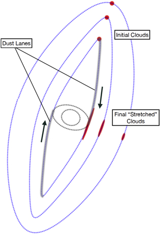
Figure 15. A cartoon image indicating the stretching of molecular gas as it travels along x1 orbits, from apocenter to pericenter. The red circles represent the initial parcels of gas located at apocenter, and the red ellipses represent their elongated counterparts once they reach pericenter. The blue dotted lines indicate various x1 orbits, and the black dotted lines indicate x2 orbits. The shaded gray regions indicate possible dust lane placements. The black arrows show the direction of gas flow. The x1 and x2 orbits, as well as the factor by which the gas is stretched, were calculated using the same gravitational potential as used in Sormani et al. (2018; their orbits are shown in the top left panel of their Figure 8).
Download figure:
Standard image High-resolution image4.3. Open Questions and Future Directions
Based on the analysis presented in this paper, we speculate that these filaments were formed due to accelerations imposed by the Galaxy bar potential. To fully test this prediction, it will be important to determine if these filamentary structures are observed elsewhere in the Sgr E complex. This could be done by completing multiple observations surveying a larger portion of the Sgr E region at a comparable spatial resolution. In addition to this, it would be useful to expand the target region to see the full lengths of the filaments. Another strong test of our dynamical origin prediction would be to make similar observations toward the ending portion of the near dust lane. Observing a pervasive population of molecular filaments with orientations and physical properties similar to the filaments reported on in this paper would support our hypothesis that the molecular gas in the Sgr E region is being stretched into filaments along its orbital path due to the gravitational influence from the Galactic bar. It would also be informative to compare these observations with hydrodynamical simulations of comparable resolution to see if such filamentary structures are formed in regions analogous to the location of Sgr E.
5. Conclusion
Sgr E is a unique and dynamic H ii region complex that is situated at the intersection between the CMZ and the far dust lane. With our analysis of new ALMA data, we have shown the following.
- 1.We observe two prominent and distinct filaments in p–p–v space within the small part of the Sgr E region targeted in our ALMA observations. These filaments are seen clearly in the 12CO, 13CO, and C18O emissions, and we refer to them as filaments 1 and 2.
- 2.These two filaments have measured lengths of at least ∼2 pc and FWHM widths of ∼0.1 pc.
- 3.Both filaments are aligned nearly parallel to the Galactic plane, with position angles ∼2°.
- 4.Filaments 1 and 2 have central velocities of −223 km s−1 and −203 km s−1, respectively.
- 5.There are two other line-of-sight velocity components centered at −209 km s−1 and −219 km s−1, which are observed along the lengths of filament 1 and 2, respectively. We determine that these components are not directly associated with filaments 1 and 2, but are likely associated with either local nonfilamentary emission in the field of view or a separate coherent structure that is cospatial with the identified filament regions.
- 6.Filaments 1 and 2 have velocity gradients <1 km s−1 pc−1, within the expected range for filaments found in typical Galactic environments.
- 7.Both filaments have FWHM velocity line widths of ∼2.0 km s−1. These line widths are narrow when compared to those measured in the CMZ, and are similar to those measured in the Galactic disk on comparable scales.
We propose that the physical and kinematic properties of these filaments can be explained by considering the location and dynamics of the Sgr E region with respect to the Galaxy. The elongation and orientation of our filaments might be caused by the "stretching" of molecular gas in Sgr E, due to the gravitational influence of the Galactic bar. Further investigation is needed to support or refute this line of reasoning. It would be useful to observe the CO emission toward other pointings in the Sgr E complex and in the analogous portion of the near dust lane, at a similar resolution and with a larger field of view. Identifying other filaments with similar properties to those reported here would provide important insights into the larger-scale gas motions that occur between the Galactic bar dust lanes and the CMZ, and how they affect the small-scale gas motions in this region.
J.W. gratefully acknowledges funding from the National Science Foundation under Award No. 2108938.
C.B. gratefully acknowledges funding from the National Science Foundation under Award Nos. 1816715, 2108938, and CAREER 2145689, as well as from the National Aeronautics and Space Administration, through the Astrophysics Data Analysis Program, under Award No. 21-ADAP21-0179, and through the SOFIA archival research program, under Award No. 09_0540.
Financial support for this work was provided by NASA through award No. 09_0540, issued by USRA.
Support for this work was provided by the NSF through award No. SOSPA7-007, from the NRAO.
M.C.S. acknowledges financial support from the European Research Council, via the ERC Synergy Grant "ECOGAL Äì Understanding our Galactic ecosystem: from the disk of the Milky Way to the formation sites of stars and planets" (grant No. 855130).
A.T.B. would like to acknowledge funding from the European Research Council (ERC), under the European Union's Horizon 2020 research and innovation program (grant agreement No. 726384/Empire).
S.C.O.G. acknowledges support from the Deutsche Forschungsgemeinschaft (DFG) via SFB 881, "The Milky Way System" (Project-ID 138713538; subprojects B1, B2, and B8), and from the Heidelberg cluster of excellence EXC 2181-390900948, "STRUCTURES: A unifying approach to emergent phenomena in the physical world, mathematics, and complex data," funded by the German Excellence Strategy. He also acknowledges funding from the ERC via the ERC Synergy Grant ECOGAL (grant No. 855130).
A.G. acknowledges support from the NSF under awards AST 2008101 and and CAREER 2142300.
The National Radio Astronomy Observatory is a facility of the National Science Foundation, operated under cooperative agreement by Associated Universities, Inc.
This paper makes use of the following ALMA data: ADS/JAO.ALMA#2019.1.01240.S. ALMA is a partnership of ESO (representing its member states), NSF (USA), and NINS (Japan), together with NRC (Canada), MOST and ASIAA (Taiwan), and KASI (Republic of Korea), in cooperation with the Republic of Chile. The Joint ALMA Observatory is operated by ESO, AUI/NRAO, and NAOJ.
Facility: ALMA.
Software: Astropy (Astropy Collaboration et al. 2013, 2018), Spectral Cube (Ginsburg et al. 2019), Radfil (Zucker & Chen 2018), Filfinder (Koch & Rosolowsky 2015), pvextractor (Ginsburg et al. 2016a), CASA: versions 5.6.1–8 (McMullin et al. 2007).
Appendix A: Velocity Channel Maps for the Spectral Lines 12CO and C18O
For completeness, we include the full-resolution velocity channel maps for the spectral lines 12CO and C18O (Figures 16 and 17). These channel maps have the same channel widths (∼0.3 km s−1) and cover the same velocity ranges as the 13CO channel maps presented in Figure 4.
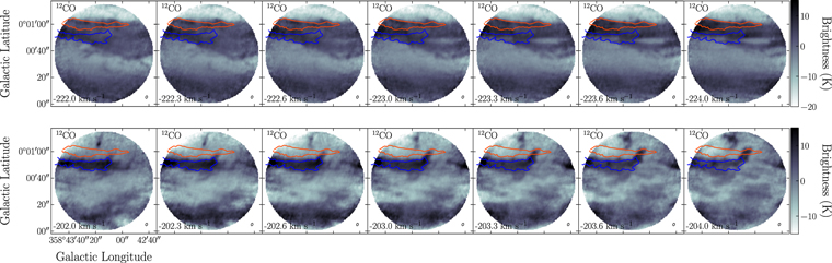
Figure 16. The full-resolution velocity channel maps for the spectral line 12CO, with channel widths of ∼0.3 km s−1. The channel maps on the top row span the velocity range of −222.0 km s−1 to −224.0 km s−1. The channel maps on the bottom row span the velocity range of −202.0 km s−1 to −204.0 km s−1. In each figure, the top—orange—contour indicates the region that we define for filament 1, while the bottom—blue—contour indicates the filament 2 region. The beam is indicated in the lower right corner of each channel map.
Download figure:
Standard image High-resolution image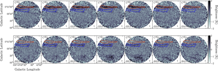
Figure 17. The full-resolution velocity channel maps for the spectral line C18O, with channel widths of ∼0.3 km s−1. The channel maps on the top row span the velocity range of −222.0 to −224.0 km s−1. The channel maps on the bottom row span the velocity range of −202.0 km s−1 to −204.0 km s−1. In each figure, the top—orange—contour indicates the region that we define for filament 1, while the bottom—blue—contour indicates the filament 2 region. The beam is indicated in the lower right corner of each channel map.
Download figure:
Standard image High-resolution image
Appendix B: Estimation of Uncertainty
The primary sources of error for the filament width and velocity line width calculations arise from the choices of fitting distance and background subtraction radius when generating a Gaussian fit. The RadFil Python package has a built-in method for estimating this systematic uncertainty, which is described in detail in Zucker & Chen (2018). In short, this method requires that the user inputs a range of fitting distances and background subtraction radii. These inputs then allow Radfil to calculate the best fit to the data using all possible combinations. The overall systematic error is then calculated by taking the standard deviation of the resulting ensemble of best-fit parameters.
For the Gaussian fits of the filament profiles, we used fitting distances of 0.025 pc, 0.050 pc, 0.075 pc, and 0.10 pc, and background subtraction radii with an inner bound of 0.25 pc and outer bounds of 0.6 pc, 0.8 pc, 1.0 pc, and 1.2 pc. For the Gaussian fits of the velocity component profiles, we used fitting distances of 1.0 km s−1, 1.3 km s−1, 1.7 km s−1, and 2.0 km s−1, and background subtraction radii with an inner bound of 2.7 km s−1 and outer bounds of 6.7 km s−1, 10.0 km s−1, 13.3 km s−1, and 20.0 km s−1. The systematic uncertainties for the filament widths and the velocity component line widths are reported in Tables 2 and 3, respectively.
Footnotes
- 9
With respect to the C18O spectral line.
- 10
A voxel is a unit for a three-dimensional data set, with two axes corresponding to spatial coordinates, in this case Galactic, and the third being a frequency or velocity axis.
- 11
- 12
- 13
See Hacar et al. (2022, Section 2) for the calculation of σtot.