


Abstract
Solar-cycle-related variation of the solar chromospheric rotation is studied by analyzing the chromospheric rotation rate of 938 synoptic maps generated from the Ca ii K line at the Mount Wilson Observatory during the period of 1915 August 10 to 1985 July 7. The results obtained are as follows: (1) The parameters A (the equatorial rotation rate) and B (the latitudinal gradient of rotation) in the standard form of differential rotation both show a decreasing trend in the considered time frame, although A has weak statistical significance. (2) There is a significant negative correlation between the level of solar activity and parameter B, indicating that there seems to be a correlation between field strength and chromospheric differential rotation. (3) During solar cycles 15, 16, 19, 20, and 21, the southern hemisphere rotates faster, whereas in cycles 17 and 18, the northern hemisphere rotates faster. (4) There exists a significant negative correlation between the N–S asymmetry of the chromospheric rotation rate and that of solar activity, indicating that differential rotation of the chromosphere seems to be strengthened by stronger magnetic activity in a certain hemisphere. Possible explanations for the above results are given.
Export citation and abstract BibTeX RIS

Original content from this work may be used under the terms of the Creative Commons Attribution 4.0 licence. Any further distribution of this work must maintain attribution to the author(s) and the title of the work, journal citation and DOI.
1. Introduction
Solar differential rotation is an important ingredient in explaining the characteristics of solar cycles in solar dynamo models (Babcock 1961; Dikpati & Gilman 2006; Cameron et al. 2017; Javaraiah 2020). The nature of solar cycles is magnetic, and the combination of the solar rotation profile and the interplay between meridional circulation, the movement of flux tubes through the convection zone, and the production of a magnetic field in the tachocline zone are thought to be responsible for solar cycles (Durney 2000; Ossendrijver 2003; Miesch 2016; Bertello et al. 2020). Therefore, studying variations in solar differential rotation is of great significance for better understanding the physical mechanism of solar cycles and other changes in solar activities.
Many authors have studied the solar differential rotation by using different data and methods. For example, the Greenwich data set and the extended Greenwich data set, consisting of sunspots and sunspot groups, were used by Balthasar & Woehl (1980), Arevalo et al. (1982), Balthasar et al. (1986), Pulkkinen & Tuominen (1998), Javaraiah (2003), Zuccarello & Zappalá (2003), Javaraiah (2005), Brajša et al. (2006), and Li et al. (2011, 2014); the sunspots and sunspot-group data set from the Solar Observing Optical Network/United States Air Force/National Oceanic and Atmospheric Administration (SOON/USAF/NOAA) was used by Pulkkinen & Tuominen (1998), Javaraiah (2013), and Ruždjak et al. (2017); and the sunspot groups from the Kanzelhhe (KSO) data set and the Mount Wilson data set (MWO) were used by Lustig (1983), Howard (1984), Hathaway & Wilson (1990), Poljančić et al. (2017), Ruždjak et al. (2017), and Poljančić et al. (2022). The X-ray bright points (XBPs) and coronal holes (CHs) in SOHO/EIT (Solar and Heliospheric Observatory/Extreme ultraviolet Imaging Telescope) images were used by Brajša et al. (2002), Brajša et al. (2004), Karachik et al. (2006), Wohl et al. (2010), Jurdana-Šepić et al. (2011), and Hiremath & Hegde (2013), and the XBPs and the small bright coronal structure (SBCS) in Hinode/XRT (X-Ray Telescope) and Yohkoh/SXT (Soft X-ray Telescope) images were used by Weber et al. (1999), Kariyappa (2008), Hara (2009), and Chandra et al. (2018).
More authors have mainly studied the relationship between solar differential rotation and solar cycles in the photosphere and in the corona. Variations of the chromospheric rotation in solar cycles are rarely mentioned. The main reasons for the relatively less well-determined chromospheric rotation are as follows: (i) some types of long-lived tracers are less prominent in the chromosphere, and (ii) long-lived tracers are not easy to distinguish in long-term observations of the chromosphere (Xiang et al. 2020; Xu et al. 2020). Long ago, Antonucci et al. (1979a, 1979b) investigated the effect of the lifetime and size of feature tracers on the chromospheric rotation. They found that short-lived tracers of the chromospheric Ca ii K line rotate more differentially during the declining solar activity than the long-lived ones, and the smaller the size of chromospheric features, the faster the rotation rate. In recent years, Li et al. (2020) studied differential rotation of the solar chromosphere using Carrington synoptic maps obtained in the spectrum of the chromosphere absorption line He i 10830. They found that both the chromosphere and the quiet chromosphere rotate faster than the quiet photosphere, and large-scale magnetic fields are correlated with the chromospheric differential rotation rate. Xu et al. (2020) investigated differential rotation of solar chromospheric activity from a global perspective using the Mg ii index, and found that the time-varying rotational period length of the chromosphere shows a declining trend during the last four solar cycles, presumably due to a decreasing strength of solar activity. However, because the duration of the data they used is not long enough (they contain four solar cycles at most), the long-term variations of solar chromospheric rotation and its relationship with solar cycles is not well-understood. Therefore, more research on these topics is highly warranted.
In the last ten years, the historical database of Ca ii K lines from the Mount Wilson Observatory has been organized (Bertello et al. 2010, 2014, 2020). The Ca ii K line (393.367 nm) is not only among the strongest and broadest lines in the visible solar spectrum but is also the most typical emission line to study long-term solar chromospheric activities, although it is in the violet part of the solar spectrum (Schrijver et al. 1989; Donahue & Keil 1995; Foukal et al. 2006; Ermolli et al. 2014; Balogh et al. 2015; Bertello et al. 2020; Chowdhury et al. 2022). Its intensity is a good proxy for measuring the chromospheric emission and the total solar magnetic flux (Foukal et al. 2009; Chatzistergos et al. 2019; Chowdhury et al. 2022). Moreover, Ca ii K observations have been used to represent the dynamics and morphology of chromospheric activity (Bertello et al. 2020).
In order to add further information about the long-term variations and fundamental process of the solar chromospheric rotation, we analyzed this database from the Mount Wilson Observatory, which contains 938 Carrington synoptic maps of the chromosphere in the Ca ii K line from Carrington rotation 827 (1915 August 10) to 1764 (1985 July 7), including about seven solar cycles. In the next section, we give a brief introduction to the observational data and methods employed in this paper. Section 3 includes the statistical results. Finally, our conclusions and a discussion are given in Section 4.
2. Data and Methods
2.1. Data
More than 35,000 daily observed spectroheliogram images were taken in the chromospheric resonance line of Ca ii K at the Mount Wilson Observatory during the period of 1915 August 10 to 1985 July 7 (Foukal & Milano 2001; Lefebvre et al. 2005; Ermolli et al. 2009; Bertello et al. 2010; Pevtsov et al. 2016; Bertello et al. 2020). These images have been digitized, calibrated, selected, and transformed into corresponding Carrington rotation (CR) synoptic maps (Bertello et al. 2010; Sheeley et al. 2011; Bertello et al. 2014). CR synoptic maps are very beneficial when studying the dynamic behavior of solar activity and how it changes at each location on the solar surface (Chowdhury et al. 2022). Nine hundred and thirty-eight CR synoptic maps of Ca ii K normalized intensity from CR827 to CR1764 were obtained, with some data gaps from CR1147 to CR1150 (Bertello et al. 2020). They are available from the website https://doi.org/10.7910/DVN/RQSEJ8. In each CR synoptic map, longitude is divided into 360 equidistant values, and the sine of latitude is also divided into 180 equidistant values from −1 (the southern pole) to 1 (the northern pole) (Bertello et al. 2014, 2020).
In Figure 1, we present a CR synoptic map in this database to characterize the Ca ii K intensity features. As the figure displays, brightening is evident at low latitudes (± 40°). Figure 2 shows the temporal–latitudinal distribution of Ca ii K normalized intensity during the period of 1915 August 10 to 1985 July 7, spanning seven solar cycles (from cycle 15 to cycle 21), and thus there are seven butterfly patterns that can be seen at low latitudes (± 40°) and which have intensity values that are distinctly larger than those of the background. These butterfly patterns represent the active chromosphere, lying over the strong magnetic field of the photosphere. In the following research, we will only study the chromospheric rotation in the low-latitude zone (± 40°).

Figure 1. Synoptic image of Ca ii K intensity at CR 1394 (1957 November December). The two white dashed lines indicate the latitudes of ±40°.
Download figure:
Standard image High-resolution image
Figure 2. Time–latitude distribution diagram of Ca ii K normalized intensity during the period of 1915 August 10 to 1985 July 7 (CR827—CR1764). The two horizontal white dashed lines indicate the latitudes of ± 40°, and the vertical white dashed lines show the minimum epochs of solar cycles.
Download figure:
Standard image High-resolution imageTo study the characteristics of long-term variations in the chromospheric rotation and solar activity, we take advantage of the yearly mean sunspot numbers (version 2) from the Solar Influences Data Analysis Center (SIDC), which is the most commonly used measure of long-term solar activity. They can be obtained via http://sidc.oma.be. Further, to compare the north–south (N–S) asymmetry of the chromospheric rotation rate with that of solar activity, we made use of the Greenwich daily sunspot area time series of the opposite hemispheres for the same time period. They can be downloaded freely from the website http://solarcyclescience.com/activeregions.html.
2.2. Methods
As we mentioned above, there are some data gaps from CR1147 to CR1150. To ensure the Ca ii K line time series are even, these data are filled with a large negative value. To acquire the yearly rotation rate, we use the classical autocorrelation analysis method to determine the rotation period (Stimets & Londono 1982; Xu & Gao 2016; Ray et al. 2018; Li et al. 2019, 2020). Autocorrelation is the linear dependence of a variable with itself at two points in time (Box et al. 2010). The autocorrelation coefficient at lag k is given by

where xi
is the time series of length N and μ is its overall mean,  . When calculating the autocorrelation coefficient (CC), if a negative value is encountered, both it and its paired value are excluded. Therefore, the calculation of the CC is limited to available values, without applying any negative value or interpolation. For a time series of a certain latitude in a certain year, the calculated CC varies with the relative phase shift of the series relative to itself, and the rotation period is the shift value corresponding to the local maximum CC around 27 days. As an example, Figure 3 displays the calculation results of CC for a certain year obtained at four different latitudes. The Ca ii K line time series during the period of 1915 August to 1985 July contains a total of 71 yr, and we get 118 rotation periods at 118 measured latitudes within the low-latitude zone (± 40°) in each year. It should be noted that the period obtained in Figure 3 is the Carrington synodic rotation period (CR), which is defined as 27.275 days, and its corresponding rotation rate is 360° /(27.275 days), i.e., 13
 199/day. After the synodic rotation period (P) of a series is obtained, the rotation rate (R) of a certain latitude in a certain year can be calculated by this formula: R = P × 13.199 (in °/day, (Shi & Xie 2013; Lamb 2017; Li et al. 2019; Deng et al. 2020; Li et al. 2020)). Ultimately, we acquire 71 yearly rotation rates at each of the 118 measured latitudes.

Figure 3. Autocorrelation coefficient (CC) of the Ca ii K line time series at a certain latitude in a certain year, varying with its relative phase shift. The four panels correspond to four time series whose latitudes are shown at the top of each panel. The dashed vertical line in each panel represents the local maximum CC, and the abscissa value is the Carrington synodic rotation period (CR).
Download figure:
Standard image High-resolution imageVariation of differential rotation rate (ω(ϕ)) with latitude at middle- and low-latitude zones is traditionally expressed by the standard formula (Newton & Nunn 1951)

where ω(ϕ) is the solar sidereal angular velocity at latitude ϕ, the parameter A represents the equatorial rotation rate, and the parameter B is the latitudinal gradient of rotation (Howard 1984). We make use of this formula to fit the yearly rotation rate of the Ca ii K line time series that we have obtained via the above autocorrelation method. Figure 4 shows the cross-correlation coefficient of the formula fitting to the latitudinal distribution of the yearly rotation rate. From the figure, we can see that all calculated correlation coefficients are larger than the critical value for the correlation coefficient at a 95% confidence level, except for the year of 1933, which means the formula can statistically fit the yearly rotation rate well. The fitting values of A and B for the year of 1933 are substituted by linear interpolation of their adjacent two points. It is very clear that the correlation is higher in the maximum year of a solar cycle than the corresponding minimum year.
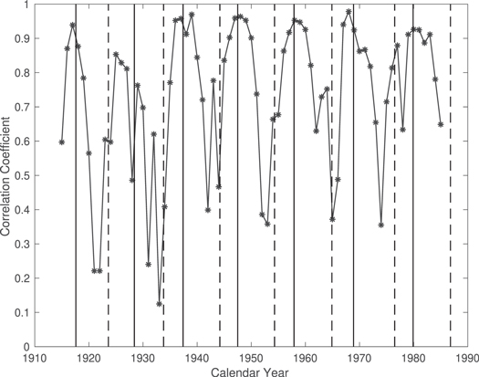
Figure 4. Correlation coefficient (asterisks) when the latitudinal distribution of the yearly rotation rate within ± 40° latitudes belt is fitted by the standard formula of solar differential rotation. The vertical dashed/solid lines show the minimum/maximum years of solar cycles.
Download figure:
Standard image High-resolution image3. Results
3.1. Solar-cycle-related Variation of Rotation Parameters A and B
Variation of the parameters A and B within solar cycles is shown in Figure 5. The parameter A is found to present a long-term weak downward trend, but the correlation coefficient from a linear fitting is −0.027, without statistical significance. The average value of A over all solar cycle maxima (13.496 (± 0.084) deg/day) is found to be slightly larger than that of all solar cycle minima (13.450 (± 0.073) deg/day). Also, a linear fitting to the parameter B over time t (years) yields B = 9.0916 − 0.0057 × t, with a correlation coefficient of 0.244, which is statistically significant at the 95% confidence level, thus the parameter B shows a relatively obvious decreasing trend. The average value of B over all solar cycle maxima (−2.468 (± 0.656) deg/day) is found to be slightly smaller than that over all solar cycle minima (−2.140 (± 0.883) deg/day).

Figure 5. Top panel: parameter A (black solid line) when the latitudinal distribution of the yearly rotation rate is fitted by the general expression of differential rotation:  . The red solid line represents the linear fitting of parameter A. Middle panel: parameter B (the black solid line) of the solar differential rotation at each year of the considered time frame. The red solid line represents the linear fitting of parameter B. Bottom panel: the yearly mean sunspot number (black solid line) in the considered time frame. The red solid line represents the linear fitting of the yearly mean sunspot number. In all panels, the black vertical dashed/solid lines indicate the minimum/maximum years of solar cycles.
Download figure:
Standard image High-resolution imageWe display the variation of the yearly mean sunspot numbers within solar cycles in the bottom panel of Figure 5. The linear fitting of the yearly mean sunspot numbers over time shows a relatively slight increasing trend. By comparing the relationship of each of parameters A and B to the yearly mean sunspot numbers, we find that there is a significant positive correlation relationship between parameter A and the yearly mean sunspot numbers, with a correlation coefficient of 0.347. However, parameter B has a significant negative correlation with the yearly mean sunspot numbers, with a correlation coefficient of −0.388. That is, the magnetic field is stronger and the parameter B is smaller, clearly indicating that there seems to be a correlation between field strength and chromospheric differential rotation, in sharp contrast to what happens in the photosphere. In the photosphere, the strong magnetic field should suppress differential rotation (Brajša et al. 2006; Wohl et al. 2010; Li et al. 2013a, 2013b).
According to the obtained parameters A and B, we utilize the standard formula to calculate the latitudinal distribution of the yearly rotation rate within a ± 40° latitude belt in the considered time frame, as shown in Figure 6. The rotation rate has a distinct characteristic of migration during a solar cycle. Figure 7 displays four isopleth lines of rotation rates, and their corresponding rotation rates are 13.3, 13.1, 12.9, and 12.7 (deg/day) from low to high latitudes. Combining Figures 6 and 7, we find that the migration of rotation rates seems to be hindered in the descending phase of a solar cycle, which is a dramatic contrast to the oscillation pattern of solar surface differential rotation (Snodgrass 1987; Li et al. 2013b).
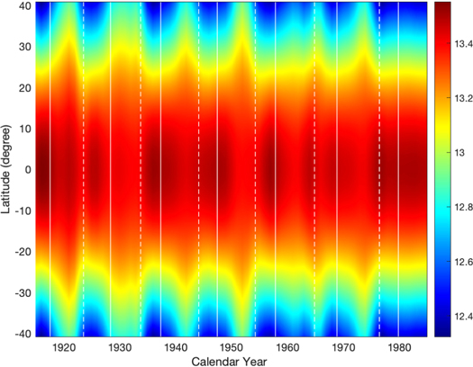
Figure 6. The latitudinal distribution of the yearly rotation rate given by the general expression of differential rotation. The unit shown on the color bar is deg/day. The white vertical dashed/solid lines indicate the minimum/maximum years of solar cycles, respectively.
Download figure:
Standard image High-resolution image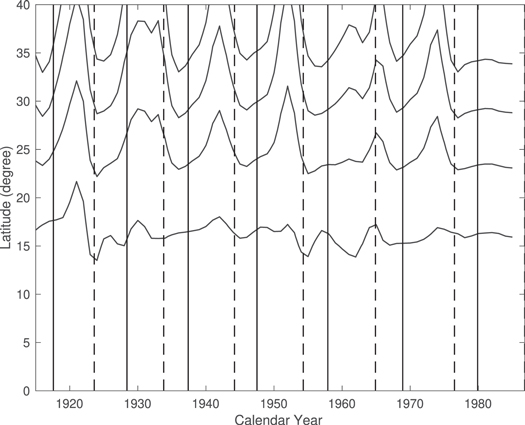
Figure 7. Isopleth lines (black solid lines) of rotation rates. The corresponding rotation rates are 13.3, 13.1, 12.9, and 12.7 (deg/day) from low latitude to high latitude. The vertical dashed/solid lines indicate the minimum/maximum years of solar cycles.
Download figure:
Standard image High-resolution imageTo study the change of parameter B over different phases of a solar cycle, we calculate the average value of B for all considered time frame within the same solar cycle phase relative to the respective minimum/maximum years of the nearest solar cycle, and its corresponding standard errors. The results are shown in Figure 8. As the figure displays, the absolute value of B increases continuously in the first three years of a solar cycle, peaks around the maximum time, then decreases slowly from the third year to the eighth year, and finally slowly increases again from the eighth year to the end of the solar cycle, clearly indicating a negative correlation between the parameter B and solar magnetic field. Therefore, there seems to be a correlation between field strength and chromospheric differential rotation. Such a solar-cycle phase of the parameter B in the chromosphere is clearly different from that in the photosphere, indicating that the effect of magnetic fields on differential rotation is different in the two atmosphere layers. In the photosphere, parameter B is weakly correlated to solar cycles and changes little during the ascending phase of a solar cycle. The absolute value of B is large, but the rotation rate on average is generally small. Therefore, the negative correlation implies that, on the whole, the stronger magnetic field is, the slower rotation rate is. As Figure 7 shows, at a certain latitude, the rotation rate is generally smaller around the maximum time of a solar cycle than in the rest time of the solar cycle.

Figure 8. Top/bottom panels: the mean value of the parameter B (the black line) depending on the phase of the solar cycle relative to the minimum/maximum years of the nearest solar cycle, and their corresponding standard errors (blue lines)
Download figure:
Standard image High-resolution image3.2. North–South Asymmetry in the Chromospheric Rotation
Many kinds of solar activities appear unevenly in the two hemispheres. This feature is known as the hemispheric north–south (N–S) asymmetry, which was first found by Spoerer (1889) through the long-term observations of sunspots. A number of authors have found the N–S asymmetry to exist in solar differential rotation (Gilman & Howard 1984; Antonucci et al. 1990; Hathaway & Wilson 1990; Javaraiah & Gokhale 1997; Brajša et al. 2000; Gigolashvili et al. 2005; Vats & Chandra 2011; Li et al. 2013a; Zhang et al. 2015; Bagashvili et al. 2017; Xie et al. 2018; Sharma et al. 2020; Hrazdíra et al. 2021; Edwards et al. 2022). Therefore, it is important to study the temporal variation of the N–S asymmetry of solar differential rotation rates, not only to provide clues to better understand the underlying mechanisms of solar cycles but also to study the N–S asymmetry of solar activities. Next, we will investigate the N–S asymmetry of the chromospheric rotation rate and its relation to the N–S asymmetry of solar activity.
To more clearly represent the rotational asymmetry, we utilize the same second-order polynomial that is used by Li et al. (2013a) to fit the latitudinal distribution of the chromospheric rotation rate:

where C0, C1, and C2 are the polynomial coefficients, ϕ is latitude in the southern hemisphere (negative values) and the northern hemisphere (positive values), ω(ϕ) is the rotation rate at a latitude ϕ, and C1 is here defined as the "asymmetry coefficient." When C1 is positive (negative), it means that the northern (southern) hemisphere should rotate faster than the southern (northern) hemisphere, and that the differential of rotation rate is more obvious in the southern (northern) hemisphere than that in the northern (southern), correspondingly.
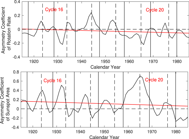
The result obtained is shown in the top panel of Figure 9. During cycles 15, 16, 19, 20, and 21, the southern hemisphere rotates faster, whereas in cycles 17 and 18, the northern hemisphere rotates faster. The degree of asymmetry during the minima of solar cycles is generally higher than that during the maxima of the solar cycle. Furthermore, to understand the evolution trend of the "asymmetry coefficient" in the considered time frame, the linear fitting method is used to fit the asymmetry coefficient, and the result presents a long-term downward trend. The correlation coefficient of 0.197 is below the 95% confidence level.
Figure 9. Top panel: variation of the asymmetry coefficient of the chromospheric rotation rate with time is shown as the black solid line, with its trend indicated by the red line. Bottom panel: variation of the normalized asymmetry index of the hemispheric sunspot area with time is shown as the black solid line, with its trend indicated by the red line. In all panels, the black vertical dashed/solid lines indicate the minimum/maximum years of solar cycles.
Download figure:
Standard image High-resolution image
To study the relationship between the N–S asymmetry of the chromospheric rotation and that of solar activity, we calculate the yearly N–S asymmetry value of the Greenwich daily sunspot area time series of the opposite hemispheres for the same time period. The N–S asymmetry is defined by the normalized asymmetry index (NAI), which was first proposed by Newton & Milsom (1955): Nasy= (N − S)/(N + S), where N and S stand for the yearly numbers of sunspot areas in the northern and southern hemispheres, respectively. The obtained values are plotted in the bottom of Figure 9. In fact, Li et al. (2002) have determined the dominant hemisphere of sunspot area in solar cycles 12–23: they found that, during cycles 15, 16, 19, and 20, the northern hemisphere dominates, whereas for the rest of the cycles, such as 17, 18, and 21, it is uncertain which hemisphere is dominant. The N–S asymmetry of sunspot area is found to present a long-term weak downward trend in the considered time frame by the linear fitting, but the correlation coefficient is 0.135, below the 95% confidence level.
Comparing the two panels of Figure 9, we find that there exists a significant negative correlation between the N–S asymmetry of the chromospheric rotation rate and that of solar activity over the considered time frame, and their correlation coefficient is −0.337, which is statistically significant at the 95% confidence level. Such a negative correlation is significantly reflected in the fact that C1 is a negative value when asymmetry of sunspot activities is a large positive value. This indicates that the differential of the rotation rate is more obvious in the northern hemisphere than in the southern, and that on the whole, the rotation rate is greater in the southern hemisphere than that in the northern, when the magnetic field strength is clearly larger in the northern hemisphere than that in the southern. This implies that there seems to be a correlation between field strength and chromospheric differential rotation.
4. Conclusion and Discussion
In this study, we used 938 Carrington synoptic images of the chromospheric Ca ii K resonance line from the Mount Wilson Observatory during the period of 1915 August 10 (CR827) to 1985 July 7 (CR1764) at a low-latitude belt (± 40°) to analyze the long-term variations in the chromospheric rotation. First, we utilized the classical autocorrelation analysis method to determine the yearly rotation period for the considered time frame and obtained the corresponding rotation rate. Then, we applied the standard formula of solar differential rotation to fit the rotation rate to get rotation parameters A and B for each year. Based on the result, we investigated the solar-cycle-related variation of rotation parameters A and B, as well as its relation to solar activity. At the same time, we studied the relationship between the latitudinal distribution of the yearly rotation rate by fitting the standard formula and solar cycles for the considered time frame. Finally, we investigated the N–S asymmetry of the chromospheric rotation rate and its relation to the N–S asymmetry of solar activity.
There is an interesting dependence of the parameter B on different phases of a solar cycle. The absolute value of B increases continuously in the first three years of a solar cycle, peaks around the maximum time, then decreases slowly from the third year to the eighth year, and finally slowly increases again from the eighth year to the end of the solar cycle, clearly indicating a negative correlation between the parameter B and solar magnetic field. Therefore, there seems to be a correlation between field strength and chromospheric differential rotation. Such a solar-cycle phase of the parameter B in the chromosphere is clearly different from that in the photosphere, indicating that the effect of magnetic fields on differential rotation is different in the two atmosphere layers. In the photosphere, the parameter B is weakly correlated to solar cycles and changes little during the ascending phase of a solar cycle (Li et al. 2013b, 2014). The absolute value of B is large, but the rotation rate on average is generally small. Therefore, the negative correlation implies that, on the whole, the stronger magnetic field is, the slower rotation rate is. We also find that rotation rate is generally smaller around the maximum time of a solar cycle than that in the rest time of the solar cycle at a certain latitude. Howard (1990) studied the variations of solar rotation velocity based on the solar active region, and found that the size of the active region is inversely related to the rotation velocity. When the observed solar surface activity becomes stronger, the rotation velocity of the solar magnetic field becomes slower. Kitchatinov et al. (1999) found a secular deceleration of solar rotation, implying a negative correlation between solar rotation rate and sunspot activity. This conclusion is also consistent with the findings of Mendoza (1999), Obridko & Shelting (2001), Brajša et al. (2007), and Obridko & Shelting (2016).
Moreover, the N–S rotational asymmetry is also investigated by fitting the latitudinal distribution of the chromospheric rotation rate with a second-order polynomial. In our study, we found that during cycles 15, 16, 19, 20, and 21, the southern hemisphere rotates faster, whereas in cycles 17 and 18, the northern hemisphere rotates faster. The degree of asymmetry during the minima of solar cycles is generally higher than that of during the maxima of solar cycles. This conclusion is consistent with Song et al. (2005), who studied the N–S asymmetry of the magnetic flux of the solar photosphere. However, Li et al. (2002) have determined the dominant hemisphere of sunspot areas in solar cycles 12–23, and found that during cycles 15, 16, 19, and 20, the northern hemisphere dominates, whereas in cycles 17, 18, and 21, it is uncertain which hemisphere is dominant. For the N–S asymmetry of the chromospheric rotation rate and solar activity, we found that there exists a significant negative correlation between the two in the long run. Zhang et al. (2013) found that the N–S asymmetry of solar rotation is anticorrelated with the area of large sunspots, and the latitudinal contrast of differential rotation also has an inverse relationship with the sunspot area. Furthermore, Zhang et al. (2015) studied the N–S asymmetry of differential rotation of solar X-ray flares and that of sunspots, and found that the southern hemisphere rotated slightly faster than the northern hemisphere. Xie et al. (2018) studied the N–S asymmetry of the rotation of the solar photospheric magnetic fields, and found that there is a significant negative correlation (at 95% confidence level) between the asymmetry of the parameter B and that of solar activity. They thought the reason for these phenomena is that differential rotation may be suppressed due to stronger magnetic activity in a certain hemisphere. In fact, the negative correlation of the N–S asymmetry of the chromospheric rotation rate and solar activity is significantly reflected in the fact that the "asymmetry coefficient" C1 is a negative value when asymmetry of sunspot activities is a large positive value. This indicates that the differential of the rotation rate is more obvious in the northern hemisphere than in the southern, and on the whole, that rotation rate is larger in the southern hemisphere than in the northern, when the magnetic field strength is clearly larger in the northern hemisphere than in the southern.This implies that there seems to be a correlation between field strength and chromospheric differential rotation, which is in agreement with the findings of Li et al. (2020).
We thank the anonymous referee for careful reading of the manuscript and constructive comments that improved the original version of the manuscript. The authors thank Professor Ke-Jun Li for his constructive ideas and helpful suggestions on the manuscript. This work is supported by the National Natural Science Foundation of China (11973085, 11903077), the Yunling-Scholar Project (the Yunnan Ten Thousand Talents Plan), the Yunnan Fundamental Research Project (202201AS070042 and 202101AT070019), the National Project for Large-scale Scientific Facilities (2019YFA0405001), and the Chinese Academy of Sciences.