Pursuing the Origin of the Gamma Rays in RX J1713.7-3946 Quantifying the Hadronic and Leptonic Components

We used archival data sets obtained with XMM-Newton to create images of synchrotron X-rays in RX J1713. We utilized the XMM-Newton Science Analysis System (SAS; Gabriel et al. 2004) version 18.0.0 and HEAsoft version 6.27.1 to analyze both the EPIC-pn and EPIC-MOS data sets with a total of 21 pointings (see Table 1). We reprocessed all the observation data files following standard procedures provided as the XMM-Newton extended source analysis software (ESAS; Kuntz & Snowden 2008). The good time intervals (GTI) after filtering soft proton flares are shown in Table 1. To generate quiescent particle background (QPB) images and exposure maps for each observation, we run the procedures "mos-/pn-back" and "mos-/pn-filter." The procedure "merge_comp_xmm" was used to combine the data from 21 pointings. Note that we excluded (1) CCD chips affected by strong stray light, especially for high energy bands, and (2) short GTI data of less than 1 ks to improve the imaging quality. Finally, we applied an adaptive smoothing using the procedure "adapt_merge", where the pixel sizes and smoothing counts were set to 6'' and 80 counts, respectively. We generated QPB-subtracted, exposure-corrected, and adaptively smoothed images in the energy bands 0.5–0.8, 0.8–1.0, 1.0–2.0, 2.0–3.0, 3.0–5.0, and 1.0–5.0 keV. 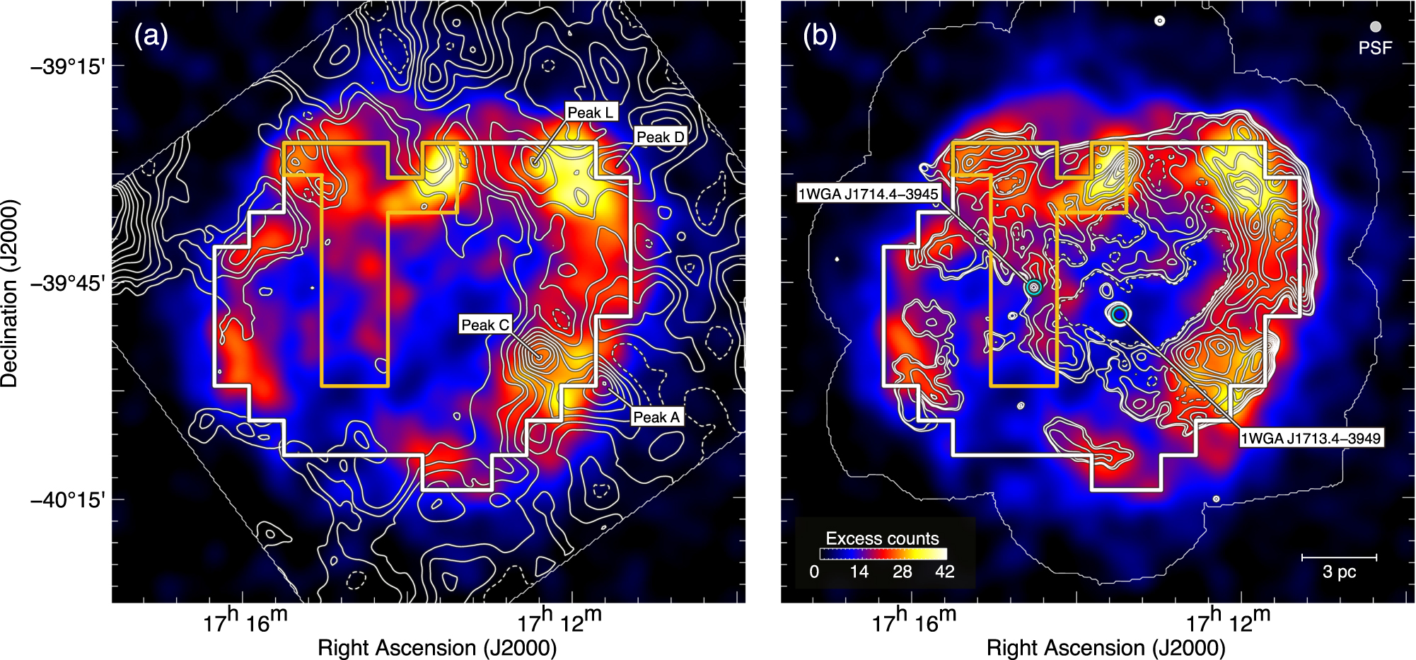⁴ Because the X-ray image in the energy band 1.0–5.0 keV is not subject to significant absorption by the ISM (see Figures 8 and 9 in Appendix B), we used the 1.0–5.0 keV image for the comparative analysis. In the present analyses, we flagged two bright point sources, 1WGA J1714.4−3945 and 1WGA J1713.4−394, considering their point-spread functions using the procedure "cheese" implemented in ESAS. We then rebinned the data to match grid size 48 of the H.E.S.S. gamma-ray data. Here we averaged data values of X-rays within each pixel area, except for the areas of the flagged point sources. The rebinned X-ray image is presented as Figure 1(b). The X-ray count N_x is given in units of 10² photons s⁻¹ deg⁻² and is used throughout the present paper.

The gamma-ray data consist of two energy ranges: above 250 GeV (broad energy band) and above 2 TeV (high energy band), which are the combined data taken in several sessions over 2004, 2005, 2011, and 2012 (H.E.S.S. Collaboration 2018). The angular resolution (FWHM) is 66 for the broad energy band and 48 for the high energy band, corresponding to spatial resolutions of 1.9 pc and 1.4 pc, respectively, at a distance of 1 kpc. We also used the previous H.E.S.S. data in Aharonian et al. (2007); the energy band is >300 GeV, similar to the broad energy band of H.E.S.S. Collaboration (2018), and the resolution is 84, corresponding to 2.5 pc.

The >2 TeV data set is named H.E.S.S.18(E > 2 TeV), which provides the highest resolution and largest number of pixels among the H.E.S.S. data available. The >250 GeV data set is named H.E.S.S.18(E > 250 GeV) and the previous H.E.S.S data are named H.E.S.S.07. In addition to H.E.S.S.18(E > 2 TeV) at $4\buildrel{\,\prime}\over{.} 8$ resolution, for testing the dependence on angular resolution and gamma-ray energy, we analyze five H.E.S.S. data sets with lower resolution as listed in Table 2; two of them are H.E.S.S.18(E > 2 TeV) smoothed to $6\buildrel{\,\prime}\over{.} 6$ resolution and H.E.S.S.18(E > 250 GeV) having $6\buildrel{\,\prime}\over{.} 6$ resolution (H.E.S.S. Collaboration 2018); the other three are H.E.S.S.18(E > 2 TeV) smoothed to $8\buildrel{\,\prime}\over{.} 4$ resolution, H.E.S.S.18(E > 250 GeV) smoothed to $8\buildrel{\,\prime}\over{.} 4$ resolution, and H.E.S.S.07 having $8\buildrel{\,\prime}\over{.} 4$ resolution. In the following analyses, all the X-ray data and the ISM data are binned to the same pixel size as the H.E.S.S. data. The gamma-ray count N_g is given in units of excess counts arcmin⁻² throughout this paper. The error was estimated as the square root of the total excess counts within each pixel in conjunction with correction for the oversampling effect.

Table 2. Summary of the Multiple Linear Regression

Data Set							F-test
Energy band	Pixel size	n	redr	a	b	R2	F	F0.01(2, n − 2)
(1)	(2)	(3)	(4)	(5)	(6)	(7)	(8)	(9)
H.E.S.S.18
E > 2 TeV	48	75	0.71	1.45 ± 0.17	1.02 ± 0.24	0.92	441.1	4.9
	66	36	0.74	1.39 ± 0.24	1.10 ± 0.34	0.97	660.0	5.3
	84	23	0.80	1.37 ± 0.28	1.05 ± 0.41	0.98	646.9	5.8
E > 250 GeV	66	36	0.74	10.6 ± 1.7	7.9 ± 2.4	0.97	641.3	5.3
	84	23	0.80	10.4 ± 1.8	8.1 ± 2.6	0.99	896.1	5.8
H.E.S.S.07
E ≳ 300 GeV a	84	23	0.80	1.87 ± 0.27	1.07 ± 0.40	0.97	383.0	5.8

Notes. Columns (1)–(3): energy band, pixel size, and number of pixels of the data set (see Section 2.2); (4) correlation coefficient between N_p and N_x; (5) and (6): regression coefficients estimated by Equation (C3) and their standard deviations (the square root of the diagonal elements of Equation (C4)); (7): coefficient of determination given by Equation (C5); (8): F-statistic given by Equation (C6); (9) critical F-value with (2, n − 2) degrees of freedom for 1% significance level. See Appendix C for further details.

^a We presumed the same energy threshold that was used for the spectral analysis in Aharonian et al. (2007).

Download table as:  ASCIITypeset image

The gamma-ray shell is peaked at ∼6 pc in radius, beyond which the gamma rays show a sharp decline. This suggests that the CR or electron energy density decreases beyond the peak (H.E.S.S. Collaboration 2018; F12). We assume that the CR energy density is nearly uniform within the shell and restrict the area of the analysis to within the gamma-ray peak. By this restriction we eliminate the outer region where the CR energy density decreases as shown by the white solid lines in Figure 1(a).

We follow F12 in calculating the ISM column density, which includes both molecular and atomic hydrogen. The molecular column density N(H₂) is calculated from the integrated intensity of the ¹²CO(J = 1–0) emission W(CO) (K km s⁻¹) for an X_CO factor 2 × 10²⁰ cm⁻² (K km s ⁻¹)⁻¹ (Bertsch et al. 1993), which is typically found in the Galaxy:

$$\begin{eqnarray}\begin{array}{rcl}{N}_{{\rm{p}}}({{\rm{H}}}_{2})\,({\mathrm{cm}}^{-2}) & = & 2\times N({{\rm{H}}}_{2})\\ & = & 4\times {10}^{20}\,W(\mathrm{CO})\,({\rm{K}}\,\mathrm{km}\,{{\rm{s}}}^{-1}).\end{array}\end{eqnarray} \tag{ 1 }$$

The atomic hydrogen column density N(H i) (cm⁻²) was calculated from the integrated intensity W(H i) (K km s⁻¹) of the 21 cm H i emission by adopting the optically thin approximation as follows:

$$\begin{eqnarray}&&N({\rm{H}}\,{\rm\small{I}})\,({\mathrm{cm}}^{-2})=1.832\times {10}^{18}\,W({\rm{H}}\,{\rm\small{I}})\,({\rm{K}}\,\mathrm{km}\,{{\rm{s}}}^{-1}).\end{eqnarray} \tag{ 2 }$$

In the present paper, we used the velocity integration range of W(CO) or W(H i) from −20 to 0 km s⁻¹, which is compatible with the previous study (F12).

Figure 1(c) shows the ISM column density distribution in units of 10²² cm⁻². We averaged values of column density within each pixel area, as with the X-ray data sets. We also correct for the H i self-absorption in the southeastern cold H i cloud by using the method in Sato & Fukui (1978), where the background H i emission is assumed to be a straight line as explained in F12. Some of the other positions may be subject to self-absorption. Figure 2 shows two cuts of H i profiles toward the region including H i with self-absorption, and indicates that a few spectra have clear dips and that some are also flat, e.g., E and F in cut 1 and cut 2. It is possible that the flat spectra are due to self-absorption, whereas there is no reliable way to assume background H i without self-absorption. If we assume a background H i emission, identical to that at position H in cut 2, we estimate that W(H i) becomes larger than in the optically thin case by a factor of 2, while the correction is arbitrary. We therefore selected 18 pixels by visual inspection as those with uncertain background emission as enclosed by the gray solid lines in Figure 1(c), and excluded them from the present analysis in order not to impair the accuracy. It is possible that the H i emission is affected by the optically thick H i (Fukui et al. 2014, 2015, 2018), whereas the direction of RX J1713 is in the Galactic plane, which does not allow us to make a direct estimate of the H i optical depth by using the Planck dust emission (Planck Collaboration 2014). We therefore did not attempt to apply the H i optical depth correction further.

Zoom In Zoom Out Reset image size

The total hydrogen column density is calculated as follows:

$$\begin{eqnarray}&&{N}_{{\rm{p}}}={N}_{{\rm{p}}}({{\rm{H}}}_{2}+{\rm{H}}\,{\rm\small{I}})=2\times {N}_{{\rm{p}}}({{\rm{H}}}_{2})\,+\,N({\rm{H}}\,{\rm\small{I}}).\end{eqnarray} \tag{ 3 }$$

Considering these ISM proton properties, we denoted the two regions as shown in Figure 1(c); the region where self-absorption is corrected for (14 pixels shown by the red solid lines) is included in the analysis, and that where correction for self-absorption is difficult due to a flat line shape, 18 pixels shown by the gray solid lines, is masked in the analysis. According to F12, the errors in the region with self-absorption are estimated to be <20%, while the errors elsewhere are mostly statistical ones and negligibly small. In Figure 1(d) we divide the pixels into five zones of N_p, which are used in Section 3. The total number of pixels after this masking is 75 in H.E.S.S.18(E > 2 TeV). A similar masking was also applied to H.E.S.S.07 and the total number of pixels is 32.

Details of the respective ISM observations are summarized below.

2.3.1. The NANTEN CO Data

2.3.2. The ATCA Plus Parkes H i Data

Motivated by the basic picture above regarding the gamma-ray origin, we formulate the gamma-ray counts as a combination of two terms, one proportional to N_p and the other proportional to N_x as a first approximation. Simple approximate relationships of N_g are given in a line of sight as follows: the number of hadronic gamma rays N_g(hadronic) via the p–p reaction is proportional to the CR proton column density N_p(CR) times the ISM proton column density N_p(ISM) (N_g(hadronic) ∝ N_p(CR) × N_p), and the number of leptonic gamma rays via the inverse Compton scattering N_g(leptonic) is proportional to the CR electron column density N_e(CR) times the uniform low-energy photon density N_photon(CMB) (N_g(leptonic) ∝ N_e(CR) × N_photon(CMB)). Noting that the nonthermal X-ray count N_x is proportional to N_e(CR) times the squared magnetic field flux density B² (N_x ∝ N_e(CR) × B²), N_g(leptonic) is hence proportional to N_x times (N_photon(CMB)/B²) (N_g(leptonic) ∝ N_x × (N_photon(CMB)/B²)) (e.g., Aharonian et al. 1997).

As a result, N_g for the combination is given by

$$\begin{eqnarray}&&{N}_{{\rm{g}}}={{aN}}_{{\rm{p}}}+{{bN}}_{{\rm{x}}},\end{eqnarray} \tag{ 4 }$$

where the coefficient a is proportional to N_p(CR) and coefficient b to N_photon(CMB)/B². Here, we can see that the coefficients a and b respectively encapsulate a global dependence on the cosmic-ray energy density and the CMB/B-field energy density ratio, as a way to provide estimates of the hadronic and leptonic fractions. We assume here that the magnetic field strength B is uniform in most of the volume as suggested by IYIF12. We consider that the CMB photon density is also uniform and that additional stellar photons are insignificant (e.g., Tanaka et al. 2008). In addition, the energy density of CRs is assumed to be uniform within the SNR shell, which is consistent with the model calculations (e.g., Zirakashvili & Aharonian 2010).

We apply Equation (4) to the data pixels in a 3D space of N_p–N_x–N_g. For this purpose, we developed the formulation for the least-squares fitting as given in Appendix C.1 in the present work and applied it to H.E.S.S.18(E > 2 TeV). As a result, we obtained a multiple linear regression plane given by the relation

$$\begin{eqnarray}&&\hat{{N}_{{\rm{g}}}}=(1.45\pm 0.17)\times {N}_{{\rm{p}}}+(1.02\pm 0.24)\times {N}_{{\rm{x}}},\end{eqnarray} \tag{ 5 }$$

for all the 75 pixels across the ISM/X-ray/gamma 3D space. The hat symbol ($\hat{}$) on N_g means that it is predicted by the regression. Table 2 lists a and b, and shows that the fitting is reasonably good with the coefficient of determination R² = 0.92 (see Appendix C.2), which means that 90% of the variance in N_g is predictable from N_p and N_x. Figure 4 shows the plane with the 75 pixels, and we confirm the good fitting. In Figure 5 we show a plot of ${\rm{\Delta }}{N}_{{\rm{g}}}={N}_{{\rm{g}}}-\hat{{N}_{{\rm{g}}}}$ as a function of $\hat{{N}_{{\rm{g}}}}$. This corresponds to a side view of the plane in Figure 4 from the direction of $\hat{{N}_{{\rm{g}}}}={\rm{constant}}$. ΔN_g is nearly zero for $\hat{{N}_{{\rm{g}}}}$ below 2.0, showing a good fit of the regression for most of the pixels. There seems to be a hint of slight decrease of ΔN_g for $\hat{{N}_{{\rm{g}}}}$ above 2.0, although the number of pixels in this range is 15. The uncertainty in $\hat{{N}_{{\rm{g}}}}$ for the ith pixel (i = 1, ⋯, 75) is given by

$$\begin{eqnarray}\begin{array}{rcl}\sigma ({\hat{N}}_{{\rm{g}},i}) & = & \left\{{\left({N}_{{\rm{p}},i}{\sigma }_{a}\right)}^{2}+{\left[a\sigma ({N}_{{\rm{p}},i})\right]}^{2}\right.\\ & & {\left.+{\left({N}_{{\rm{x}},i}{\sigma }_{b}\right)}^{2}+{\left[b\sigma ({N}_{{\rm{x}},i})\right]}^{2}\right\}}^{1/2},\end{array}\end{eqnarray} \tag{ 6 }$$

and that of ΔN_g by

$$\begin{eqnarray}&&\sigma ({\rm{\Delta }}{N}_{{\rm{g}},i})={\left[\sigma {\left({N}_{{\rm{g}},i}\right)}^{2}+\sigma {\left({\hat{N}}_{{\rm{g}},i}\right)}^{2}\right]}^{1/2}.\end{eqnarray} \tag{ 7 }$$

Here, σ(N_g), σ(N_p), and σ(N_x) are the uncertainties in N_g, N_p, and N_x, and σ_a and σ_b are the standard errors of the estimated a and b (Equation (C4) in Appendix C.1), respectively. Note that we have estimated σ(N_p,i ) from the rms noise in W(H i) and W(CO), without taking into account uncertainty in the X_CO factor.

Zoom In Zoom Out Reset image size

Zoom In Zoom Out Reset image size

Equation (5) allows us to make a first estimate of the gamma rays with hadronic and leptonic origins separately. The hadronic component is given by

$$\begin{eqnarray}&&{\hat{N}}_{{\rm{g}}}^{\mathrm{hadronic}}={{aN}}_{{\rm{p}}}\end{eqnarray} \tag{ 8 }$$

and its uncertainty is

$$\begin{eqnarray}\begin{array}{rcl}\sigma ({\hat{N}}_{{\rm{g}}}^{\mathrm{hadronic}}) & = & {\left\{{\left({\sigma }_{a}{N}_{{\rm{p}}}\right)}^{2}+{\left[a\sigma ({N}_{{\rm{p}}})\right]}^{2}\right\}}^{1/2}\\ & \sim & {\sigma }_{a}\,{N}_{{\rm{p}}},\end{array}\end{eqnarray} \tag{ 9 }$$

where we ignore the second term because σ(N_p)/N_p = 10⁻² is an order of magnitude smaller than σ_a /a. The leptonic component and its uncertainty are given in a similar manner,

$$\begin{eqnarray}&&{\hat{N}}_{{\rm{g}}}^{\mathrm{leptonic}}={{bN}}_{{\rm{x}}}\end{eqnarray} \tag{ 10 }$$

and

$$\begin{eqnarray}&&\sigma ({\hat{N}}_{{\rm{g}}}^{\mathrm{leptonic}})\sim {\sigma }_{b}\,{N}_{{\rm{x}}},\end{eqnarray} \tag{ 11 }$$

respectively. By using the coefficients a and b obtained in Section 3.1 (summarized in Table 2) and the spatially averaged gamma-ray count $\bar{{N}_{{\rm{g}}}}={\sum }_{i}{N}_{{\rm{g}},i}/n$, ISM proton column density $\bar{{N}_{{\rm{p}}}}={\sum }_{i}{N}_{{\rm{p}},i}/n$, and X-ray count $\bar{{N}_{{\rm{x}}}}={\sum }_{i}{N}_{{\rm{x}},i}/n$ listed in Table 3, it is estimated that the hadronic component constitutes (67 ± 8)% of the total gamma-ray count and the leptonic component (33 ± 8)%. Further discussion is given in Section 4.1.

Table 3. Estimate of the Gamma Rays with Hadronic and Leptonic Origin

Data Set				Hadronic Component			Leptonic Component
Energy Band	Pixel Size	$\langle \hat{{N}_{{\rm{g}}}}\rangle$	〈Np〉	${\hat{N}}_{{\rm{g}}}^{\mathrm{hadronic}}$	${\hat{N}}_{{\rm{g}}}^{\mathrm{hadronic}}/\langle \hat{{N}_{{\rm{g}}}}\rangle$	〈Nx〉	${\hat{N}}_{{\rm{g}}}^{\mathrm{leptonic}}$	${\hat{N}}_{{\rm{g}}}^{\mathrm{leptonic}}/\langle \hat{{N}_{{\rm{g}}}}\rangle$
(1)	(2)	(3)	(4)	(5)	(6)	(7)	(8)	(9)
H.E.S.S.18
E > 2 TeV	48	1.56 ± 0.02	0.72	1.04 ± 0.12	(67 ± 8)%	0.50	0.51 ± 0.12	(33 ± 8)%
	66	1.57 ± 0.04	0.73	1.01 ± 0.17	(65 ± 11)%	0.50	0.55 ± 0.17	(35 ± 11)%
	84	1.54 ± 0.07	0.74	1.01 ± 0.21	(66 ± 14)%	0.50	0.53 ± 0.20	(34 ± 13)%
E > 250 GeV	66	11.7 ± 0.3	0.73	7.7 ± 1.2	(66 ± 11)%	0.50	4.0 ± 1.2	(34 ± 10)%
	84	11.7 ± 0.4	0.74	7.6 ± 1.3	(65 ± 11)%	0.50	4.0 ± 1.3	(35 ± 11)%
H.E.S.S.07
E ≳ 300 GeV	84	1.92 ± 0.06	0.74	1.38 ± 0.20	(72 ± 11)%	0.50	0.54 ± 0.20	(28 ± 10)%

Note. Columns (1) and (2): energy band and pixel size of the data set; (3), (4) and (7): spatial averages of observed N_g (counts arcmin⁻²), N_p (10²² cm⁻²), and N_x (10² photons s⁻¹ deg⁻²), (5) and (8): predicted numbers of gamma rays with hadronic and leptonic origin (counts arcmin⁻²), (6) and (9): fractions of the hadronic and leptonic components.

Download table as:  ASCIITypeset image

We checked the effect of adding back the excluded 18 pixels and found that the fitted values for a = 1.20 ± 0.18 and b = 1.52 ± 0.24 (see Equation (4)) suggested hadronic and leptonic fractions of (52 ± 8)% and (48 ± 8)%, respectively. The hadronic fraction has decreased compared to our main result, as expected, because the lack of correction for self-absorption leads to an underestimate of N_p.

We have obtained the hadronic and leptonic gamma-ray counts in each pixel, and are able to compare (the fraction of the hadronic/leptonic gamma rays in the total gamma rays) and (N_p or N_x) over the SNR. In Figure 6, we present a scatter plot between the hadronic gamma-ray fraction and N_x in all 75 pixels for different ranges of N_p values. The hadronic fraction fitted by the model is expressed from Equation (4) as

$$\begin{eqnarray}&&\text{Hadronic gamma-ray fraction}\,=\,\displaystyle \frac{{{aN}}_{{\rm{p}}}}{{\hat{N}}_{{\rm{g}}}},\end{eqnarray} \tag{ 12 }$$

which indicates that the fraction increases with N_p and decreases with N_x. The relationships derived from Equation (12) are plotted as colored thin solid lines in Figure 6, and show a good correspondence with each pixel. The model includes both the hadronic and leptonic components, and Figure 6 naturally shows a mixed trend. We find that a high hadronic fraction of more than 70% is found toward low N_x < 0.6 and not only toward high N_p > 0.9. It is also notable that more than half of the pixels with a low hadronic fraction of less than 60% have high N_p > 0.9. These trends are likely caused by the enhanced X-rays toward dense ISM clumps. Figure 6 indicates that there are hadronic-dominated regions with fractions >70%, whereas there are no such regions dominated by leptonic emission to the same level. We also recognize these trends in Figures 7(a) and (b), which show overlays of the hadronic fraction with the distributions of N_p and N_x, respectively. The two figures are somewhat complicated to grasp simply, whereas we recognize that a high hadronic fraction is often found toward regions of low N_x, as is consistent with Figure 6; these are in the southeastern rim and in the east of the western bright X-ray shell. These comparisons will provide observational signatures of the two gamma-ray origins, which will be revealed in more depth at higher resolution in the era of the Cherenkov Telescope Array (CTA).

Zoom In Zoom Out Reset image size

Zoom In Zoom Out Reset image size

We made additional analyses of the five H.E.S.S. data sets at resolutions of 66 and 84 as listed in Table 2. The method explained in Section 3.1 is applied to them and regression flat planes derived are included in Table 2. The planes are used to derive the hadronic and leptonic gamma rays in the manner explained in Section 3.2.

In Table 3 we find that the hadronic and leptonic gamma rays show similar fractions of (65–72)%:(28–35)% or ∼6σ:3σ for each resolution. The overall results are consistent with each other and do not depend significantly on the resolution and energy. The H.E.S.S.18(E > 2 TeV) results yield hadronic and leptonic counts of ∼8σ:4σ at the highest resolution, and are of somewhat higher relative sensitivity than the results at lower resolution.

The present analysis revealed that the gamma rays in RX J1713 consist of a hadronic component and a leptonic component with a ratio of 7:3 in the gamma-ray counts. This is the first result that has quantified the two gamma-ray components, and it has opened a possibility to explore the physical processes operating in each part of the SNR. It is to be emphasized that the separation of the two gamma-ray components was achieved for the first time only by including explicitly the ISM proton column density. The hybrid origin was theoretically modeled by ZA10 (see their Figure 14). The present results indicate that the hadronic component is more significant than shown by ZA10, which assumed a small target mass of the ISM. In fact, ZA10 assumed the interacting molecular mass to be 100–1000 M_⊙, which comprises only the two individual molecular clouds C and D (Fukui 2008). The total ISM mass associated with the SNR, however, is ∼20,000 M_⊙ by summing up all molecular and atomic clouds interacting with the SNR (F12).

The principal aim of F12 was to clarify whether the target protons in the hadronic process in RX J1713 show good correspondence with the interstellar protons including H i in addition to H₂. The new feature was the inclusion of H i, and the spatial correspondence is the necessary condition of the hadronic gamma rays. It was also shown by IYIF12 that the magnetic field is likely as strong as 100 mG or higher, making the leptonic component unfavorable. Their azimuthal angle distribution of the gamma rays and ISM seems to be matched without invoking an additional contribution. ⁵ Accordingly, F12 concluded that the gamma rays are mainly of hadronic origin, while a contribution from the leptonic component was not excluded. Subsequent works on CTA simulations of the hadronic and leptonic origins pursued this issue and argued for a possibility of resolving the degeneracy originating from the shell-like distribution of the ISM and nonthermal X-rays (Acero et al. 2017). In two other TeV gamma-ray SNRs, HESS J1731−347 and RCW 86, the ISM and the nonthermal X-rays show significantly different spatial distributions, allowing one to separate the two origins (Fukuda et al. 2014; Sano et al. 2019), while another TeV gamma-ray SNR, RX J0852.0−4622, shows shell-like distributions of the ISM and nonthermal X-rays, making a case similar to RX J1713. In order to shed more light on the issue we applied the present method to the previous data H.E.S.S.07 used by F12, and find that the ratio of the hadronic and leptonic components is ∼(72 ± 11):(28 ± 10) in gamma-ray counts, which is similar to the present results. The 3σ significance of the leptonic component might place it at a marginal level, while the low spatial resolution and the small number of data pixels would make the analysis of H.E.S.S.07 crude at best.

A further issue is the possible suppression of the gamma rays by second-order effects that may make the gamma rays deviate from a simple proportionality to N_p or N_x. Such effects include the shock–cloud interaction and the penetration depth. Some other effects such as secondary particle acceleration may be operating, as suggested by Aharonian (2004), while these effects are not yet fully investigated/confirmed theoretically or observationally; such mechanisms include second-order Fermi acceleration (Fermi 1949), magnetic reconnection in the turbulent medium (Hoshino 2012), reverse shock acceleration (e.g., Ellison 2001), and the nonlinear effect of DSA (e.g., Malkov & Drury 2001). We shall not discuss them in the present paper.

IYIF12 made MHD numerical simulations of the shock front interacting with the clumpy ISM. Recent MHD simulations of dense cores overtaken by the shock by Celli et al. (2019) for a more realistic core density above that of IYIF12 confirmed the results of IYIF12. The interaction produces a highly turbulent velocity field around the dense cores, which amplifies the magnetic field up to 100 μG–1 mG. The effects are observationally confirmed by rim-brightened X-rays for a typical radius of the dense cores of 0.5 pc by Sano et al. (2013) through a detailed comparative study of the ISM and X-rays. The ∼100 μG B field will deplete CR electrons by synchrotron cooling and can lead to suppression of the leptonic gamma rays.

Gamma rays of hadronic origin are not always perfectly proportional to the ISM column density because CRs cannot penetrate freely into the dense cores, as pointed out by Gabici et al. (2007) and IYIF12. The expression for the penetration depth of CR protons into dense cores is given as follows (IYIF12):

$$\begin{eqnarray}\begin{array}{rcl}{l}_{\mathrm{pd}}\,(\mathrm{pc}) & = & 0.1\,{\eta }^{1/2}{\left(\displaystyle \frac{E}{10\mathrm{TeV}}\right)}^{1/2}\\ & & \times \ {\left(\displaystyle \frac{B}{100\mu {\rm{G}}}\right)}^{-1/2}\left(\displaystyle \frac{{t}_{\mathrm{age}}}{{10}^{3}\,\mathrm{yr}}\right),\end{array}\end{eqnarray} \tag{ 13 }$$

where l_pd is the penetration depth of cosmic rays, η is the CR gyro-factor, E is the cosmic-ray energy, B is the magnetic field strength, and t_age is the age of the SNR. If we adopt E = 10 TeV, ⁶ t_age = 1600 yr, B = 100 μG (Celli et al. 2019), and η = 1 (e.g., Tanaka et al. 2008; Tsuji et al. 2019), we estimate l_pd = 0.13 pc. The dense cores in RX J1713 have a typical radius of ∼0.5 pc (Sano et al. 2010, 2013) and l_pd is small enough to affect the CR injection into them. Here, the volume filling factor of the dense cores in RX J1713 is ∼10% by assuming 22 molecular clouds with typical radii of ∼1.4 pc and the SNR shell radius of 9 pc (Sano et al. 2013). The gamma-ray suppression is therefore not likely to be dominant overall.

Recently, Sano et al. (2020) revealed a high-resolution distribution of CO with the Atacama Large Millimeter/submillimeter Array (ALMA) toward part of the peak D cloud, and a small-scale (0.1–0.02 pc) clumpy distribution has been revealed. If such a highly clumpy distribution is common in the ISM, CRs may more easily penetrate into dense ISM and may increase the hadronic gamma rays more than inferred from an unresolved ISM distribution. So, it will be important to resolve the ISM at a sub-parsec scale in order to better understand the hadronic gamma rays.

In either case, the suppression is supposed to appear at high N_g, and the slight decrease of ΔN_g in only three pixels at around 2.5σ level in Figure 5 might be caused by these effects. The three pixels are indicated by green lines in Figure 1(a). This issue is to be clarified by future, more sensitive observations. Overall, the present methodology appears to describe the general behavior of N_g.

The present work used the ISM distribution consisting of both atomic and molecular hydrogen (F12). A problem we faced is that the accuracy of estimating N(H i) is limited by the H i self-absorption. By new identification of possible self-absorption in H i, we excluded 18 pixels from the analysis, where self-absorption effects are suspected. Since the accuracy in correction for self-absorption is limited by the uncertainty in the assumed H i background emission, it is impossible to achieve accuracy better than ∼20% for a correlation analysis if self-absorption is significant. If the correction is not adequate in some pixels of the present analysis, it leads to underestimation of the ISM column density and ${\hat{N}}_{{\rm{g}}}$ as well. Then, ΔN_g becomes overestimated in Figure 5. The four pixels with a deviation of more than 2.5σ in the range $\hat{{N}_{{\rm{g}}}}$ = 1.0–2.0 may show such a case. In order to correct such inaccuracies, we need to develop a new tracer for both H i and H₂. Inoue & Inutsuka (2012) made numerical simulations of the magnetohydrodynamics of colliding H i flows and traced the H i evolution leading to H₂ cloud formation. By synthetic observations of the numerical results of Inoue & Inutsuka (2012), Tachihara et al. (2018) and Fukui et al. (2018) show that the submillimeter transition of neutral carbon C i is a good tracer of all ISM protons (H i + H₂) in a density regime around 10³ cm⁻³ (see Figure 8 of Tachihara et al. 2018). We suggest that C i could serve as a useful probe of ISM protons in future and may become a promising tool in an ISM study of SNRs. This is particularly relevant in the CTA era, where more SNRs in the Galactic plane, subject to strong H i absorption, will be discovered.

Once a supernova occurs, CRs are accelerated by DSA in the SNR. Nonthermal X-rays are emitted by the synchrotron mechanism, and gamma rays by the p–p reaction or inverse Compton scattering. A general picture of the hadronic and leptonic gamma rays from a nonthermal X-ray SNR is that the gamma rays are proportional to either N_p or N_x. In RX J1713, the CRs are perturbed by interaction with the ISM. The distribution of the ISM is highly clumpy, with the dense cores having a small volume filling factor of ∼10% in RX J1713. The distribution was determined prior to the supernova by the cloud self-gravity, which may involve star formation as in peak C (Sano et al. 2010) and environmental effects including the progenitor's stellar winds over millions of years. Theoretical studies of the interaction show that the gamma rays and X-rays are significantly affected by the dense cores (Gabici et al. 2007; IYIF12; Celli et al. 2019). The secondary acceleration of CRs might also affect the X-rays, as suggested by a spectral analysis of X-rays by Sano et al. (2015), whereas there is no established picture for the acceleration.

The present hybrid picture is qualitatively consistent with the composite scenario by ZA10. Naturally, the fraction of leptonic gamma rays increases where the ISM density is low. In the other three TeV gamma-ray SNRs, HESS J1731−347 (HESS J1731), RX J0852.0−4622, and RCW86, spatial correspondence between the gamma rays and the ISM has been shown and the hadronic gamma rays are suggested to be dominant (Fukuda et al. 2014; Fukui et al. 2017; Sano et al. 2019). In two of them, HESS J1731 and RCW86, in a minor portion of the SNRs where the gamma-ray distribution shows correspondence with the nonthermal X-rays but not with the ISM, it is suggested that the gamma rays are mostly of leptonic origin (Fukuda et al. 2014; Sano et al. 2019). RX J1713 is a more complicated case where the nonthermal X-rays are heavily overlapped with the gamma rays and are not easily separable at the current resolution. The methodology proposed in the present work has provided a new tool to quantify the leptonic and hadronic gamma rays and will be applicable to the other SNRs. The present paper lends support to the vital role of the ISM in the production of HE and VHE energy radiation in an SNR, confirming that the inclusion of the ISM in an analysis is crucial for our understanding of the origin of the gamma rays.

Furthermore, numerical simulations of the gamma-ray spectral energy distributions in RX J1713 have been made by ZA10 as well as other authors (see references in ZA10). These simulations assumed the ratio of relativistic electrons to protons K_ep to be 10⁻² to 10⁻³ and obtained results that are not inconsistent with the present result. This suggests that the values assumed above satisfy the present requirement of the gamma-ray and X-ray results in addition to the ISM data, whereas it seems that better statistics of the gamma-ray data, which will be provided in the CTA era, would enable us to better constrain K_ep.

Equation (4) can be rewritten in a matrix form

$$\begin{eqnarray}&&\left(\begin{array}{c}{N}_{{\rm{g}},1}\\ \vdots \\ {N}_{{\rm{g}},n}\end{array}\right)=\left(\begin{array}{cc}{N}_{{\rm{p}},1} & {N}_{{\rm{x}},1}\\ \vdots & \vdots \\ {N}_{{\rm{p}},n} & {N}_{{\rm{x}},n}\end{array}\right)\left(\begin{array}{c}a\\ b\end{array}\right)+\left(\begin{array}{c}{\varepsilon }_{1}\\ \vdots \\ {\varepsilon }_{n}\end{array}\right),\end{eqnarray} \tag{ C1 }$$

or more simply

$$\begin{eqnarray}&&{\boldsymbol{y}}={\boldsymbol{Xb}}+{\boldsymbol{\varepsilon }},\end{eqnarray} \tag{ C2 }$$

where ${\boldsymbol{y}}={\left(\begin{array}{ccc}{N}_{{\rm{g}},1} & \cdots & {N}_{{\rm{g}},n}\end{array}\right)}^{{\rm{T}}}$ is a vector of n observations of the dependent variable N_g and the superscript T means transpose,

$$\begin{eqnarray*}{\boldsymbol{X}}=\left(\begin{array}{cc}{N}_{{\rm{p}},1} & {N}_{{\rm{x}},1}\\ \vdots & \vdots \\ {N}_{{\rm{p}},n} & {N}_{{\rm{x}},n}\end{array}\right)\end{eqnarray*}$$

is an n × 2 matrix where we have observations of two explanation variables, N_p and N_x, for n observations, ${\boldsymbol{b}}={\left(\begin{array}{cc}a & b\end{array}\right)}^{{\rm{T}}}$ is a vector of unknown coefficients that we want to estimate, and ${\boldsymbol{\varepsilon }}={\left(\begin{array}{ccc}{\varepsilon }_{1} & \cdots & {\varepsilon }_{n}\end{array}\right)}^{{\rm{T}}}$ is a vector of disturbances.

An estimate of the coefficients $\hat{{\boldsymbol{b}}}$ that minimize the sum of squared residuals ε ^T ε is given as

$$\begin{eqnarray}&&\hat{{\boldsymbol{b}}}={({{\boldsymbol{X}}}^{{\rm{T}}}{\boldsymbol{WX}})}^{-1}{{\boldsymbol{X}}}^{{\rm{T}}}{\boldsymbol{Wy}},\end{eqnarray} \tag{ C3 }$$

where an n × n diagonal matrix

$$\begin{eqnarray*}{\boldsymbol{W}}=\left(\begin{array}{ccc}{w}_{1} & & \\ & \ddots & \\ & & {w}_{n}\end{array}\right)\end{eqnarray*}$$

is the weight matrix, ${w}_{i}=\sigma {({N}_{{\rm{g}},i})}^{-2}$ (i = 1, ⋯, n). Here, we do not take into account σ(N_p) and σ(N_x) because they are relatively small: σ(N_p)/N_p = 10⁻² and σ(N_x)/N_x = 10⁻²–10⁻³, while σ(N_g)/N_g = 10⁻¹. The standard errors of the estimated coefficients, σ_a and σ_b , are given as the square root of the diagonal elements of a matrix

$$\begin{eqnarray}&&\displaystyle \frac{{\left({\boldsymbol{y}}-\hat{{\boldsymbol{y}}}\right)}^{{\rm{T}}}{\boldsymbol{W}}({\boldsymbol{y}}-\hat{{\boldsymbol{y}}})}{n-m}{\left({{\boldsymbol{X}}}^{{\rm{T}}}{\boldsymbol{WX}}\right)}^{-1},\end{eqnarray} \tag{ C4 }$$

where $\hat{{\boldsymbol{y}}}={\boldsymbol{X}}\hat{{\boldsymbol{b}}}={\left(\begin{array}{ccc}{\hat{N}}_{{\rm{g}},1} & \cdots & {\hat{N}}_{{\rm{g}},n}\end{array}\right)}^{{\rm{T}}}$ is a vector of predicted values of N_g and m = 2 is the number of explanation variables (N_p and N_x).

Taking into account the particularities of regression through the origin (briefly summarized in Appendix A of Legendre & Desdevises 2009), we calculate the coefficient of determination ⁷ as

$$\begin{eqnarray}&&{R}^{2}=\sum _{i=1}^{n}{\left({\hat{N}}_{{\rm{g}},i}\right)}^{2}/\sum _{i=1}^{n}{\left({N}_{{\rm{g}},i}\right)}^{2}\end{eqnarray} \tag{ C5 }$$

and the F-statistic associated with R² as

$$\begin{eqnarray}&&F=\displaystyle \frac{{R}^{2}/m}{(1-{R}^{2})/(n-m)}.\end{eqnarray} \tag{ C6 }$$

R² indicates how the variance in the dependent variable (N_g) can be explained by those in the explanation variables. It normally ranges from 0 to 1, and a high R² indicates a good fit. The derived F = 337.0 is much greater than the critical value of the F-distribution with (m, n − m) degrees of freedom, F_0.01(2, n − 2) = 4.9; therefore we can reject a null hypothesis a = b = 0, which means N_g is dependent on neither N_p nor N_x, at a significance level of 1%.

Multicollinearity is a well known problem that increases the variance of the coefficient estimates (σ_a and σ_b in the present study) and makes the estimates unstable. It occurs when the explanation variables in the regression model are highly correlated. A formal and widely accepted method for detecting the presence of multicollinearity is the use of a variance inflation factor (VIF). A VIF value greater than 10 is commonly used as an indicator of multicollinearity but a more conservative threshold of 5 or 3 is sometimes chosen.

There are only two explanation variables (N_p and N_x) in the regression model in the present study, so the VIF is given by

$$\begin{eqnarray}&&\mathrm{VIF}=\displaystyle \frac{1}{1-{r}^{2}},\end{eqnarray} \tag{ C7 }$$

where r is the correlation coefficient between N_p and N_x. A correlation coefficient of r = 0.71–0.80 gives a VIF of 2.0–2.8, which is an acceptable range.