


Abstract
We use a generic thermophysical model to study in detail the formation of water-ice frost in the near-surface layers of comet 67P/Churyumov-Gerasimenko. We show that nightly frost formation is a common phenomenon. In particular, while abrupt landscapes may be conducive to frost formation, they are not a requisite condition. We show that the process of subsurface frost formation is similar to that of the condensed ice layer, or crust, underneath. The sublimation of frost produces regular, enhanced outgassing early in the morning. In the case of 67P, this activity is subordinate to and precedes the daily peak sourced from the ice-rich layers located above the diurnal skin depth. In any case, frost activity should be a nominal component of comet water activity.
Export citation and abstract BibTeX RIS
1. Introduction
Water frost has been clearly observed on two cometary nuclei, namely, those of 9P/Tempel 1 and 67P/Churyumov-Gerasimenko (hereafter 67P; Sunshine et al. 2006; De Sanctis et al. 2015). Its formation is far more prevalent and has been substantiated or inferred on other planetary bodies, for instance, the Moon (Hayne et al. 2015; Fisher et al. 2017), Mars (Mellon & Jakosky 1993; Schörghofer & Aharonson 2005), Mercury (Paige et al. 2013), etc. During the extensive rendezvous of Rosetta with 67P, both short-lived and long-surviving surface ice had been frequently revealed in imaging observations (De Sanctis et al. 2015; Barucci et al. 2016; Oklay et al. 2017; Fornasier et al. 2017). De Sanctis et al. (2015) established the diurnal cycle of water ice in the subsurface. The frost, deposited (recondensed) near the surface layer by the rarifying yet persisting vapor flow during the night, sublimates instantly upon sunrise but could be discerned briefly along the terminator before depletion, an interpretation corroborated by model results presented therein. The phenomenon was widely observed throughout the rendezvous and seemed most distinguishable over irregular landscapes where the effects of topographic obstruction, or shadowing, are outstanding (Figure 1). On the bilobed comet, a propitious and well-reported site is the Hapi region, cradled between the two bulk masses (El-Maarry et al. 2015). Gas and dust coma simulations by Shi et al. (2018) showed that some exquisite, jetlike features of dust emissions along the morning terminators are attributed to the sublimation of frost alone (Figure 1). The ambient gas coma may be yet another source, or even driver, of frost deposition onto the surface and migration into the subsurface (Liao et al. 2018).
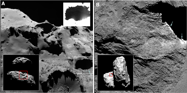
Figure 1. Frost and morning activity on the nucleus of 67P observed by Rosetta/OSIRIS. (a) Frost observed on the big lobe (highlighted by the arrow in the white rectangle). Dust activity from the frost band is seen in the contrast stretched in the upper right panel. The image was taken on 2015 January 23 at a heliocentric distance of 2.5 au inbound. (b) Frost on the small lobe along the terminator (light blue arrows). The fields of view are outlined by the red rectangles in the respective context images (lower left panels). The nucleus is roughly 4 km across. This image was taken on 2016 September 30 at an outbound heliocentric distance of 3.8 au. Credit: ESA/Rosetta/MPS for OSIRIS Team MPS/UPD/LAM/IAA/SSO/INTA/UPM/DASP/IDA. The first image is adapted from Hu et al. (2017a).
Download figure:
Standard image High-resolution imageIn this study, we concern ourselves with the behavior of frost migration in the subsurface. The general mechanism was probably responsible for the icy patches on Tempel 1 observed by Deep Impact years before (Sunshine et al. 2006). In the earliest study we have located that detailed the phenomenon, Prialnik et al. (2008) illustrated the plausible role of frost formation and sublimation in triggering some repeatedly observed "morning outbursts" on comet 9P/Tempel 1 (A'Hearn et al. 2005). The proposed mechanism for the sudden onset of activity upon sunrise preceded and was fully confirmed by the Rosetta findings. Observed in greater detail, the morning activities on 67P took a less remarkable yet still quite perceptible form of transient enhanced dust activity along the terminator with respect to the longer-illuminated surroundings (De Sanctis et al. 2015; Shi et al. 2018).
Frost formation and activity over orbital timescales were illustrated in the study of Yu et al. (2019), who investigated the thermophysical conditions for the activity of asteroid 3200 Phaethon producing the Geminid meteor showers. They showed that buildup of the dust mantle as a consequence of ice depletion in the upper subsurface yields a potential source of meteor particles; moreover, an orbital cycle of gas deposition and the subsequent intense ice sublimation at perihelion could trigger dust activity forming the tail.
Similar processes of cyclic redeposition are at work on larger objects, notably Mars, but with distinctly different material properties, atmospheric conditions, and stronger gravity (Mellon & Jakosky 1993; Schörghofer & Aharonson 2005). Nevertheless, the physical mechanisms of gas diffusion, phase change, and interactions with the ambient atmosphere, etc., governing energy distribution and material transport in the subsurface and the methodological treatment do not differ substantially from models for comets or other active small bodies.
Following these investigations, we demonstrate in this work based on a simple yet generic model that the occurrence of water frost near the subsurface is, in all likelihood, a prevalent phenomenon on comet nuclei. While its intensity must be influenced by numerous factors, for instance, local latitude, subsurface material properties, etc., the phenomenon is not restricted to abrupt landscapes with which, as it seems, frost has so far been most frequently associated. Our results conform to the findings of Prialnik et al. (2008) regarding the morning outbursts on Temple 1, triggered by exposure of nightly water frost at sunrise. In the case of 67P, where the dust mantle is only a few millimeters thick, the dominant component of the diurnal activity is still sourced from the ice-rich layers below the mantle. Frost sublimation manifests in a short-lived, lesser peak in the early morning prior to the daytime maximum and is thus principally compatible with the conclusions of De Sanctis et al. (2015) and Shi et al. (2018). We propose that the frost activity likely comprises an inherent regular component of nominal water activity on comets.
2. Thermophysical Model
The basic methodology of thermophysical modeling has been well established for decades in the cometary literature (Prialnik et al. 2004; Huebner et al. 2006). The main objective is to characterize the temperature and compositional and structural properties of the body and their evolution in response to time-varying energy input. In general, there are (at least) two fundamental equations to be formulated: (1) the heat equation accounting for conservation of the system energy and (2) a mass equation expressing the conservation of mass. Among numerous studies based on more or less the same treatment, we refer to, by no means exhaustively, the following: Mekler et al. (1990), Spohn & Benkhoff (1990), Kömle & Steiner (1992), Orosei et al. (1995), Enzian et al. (1997), Davidsson & Skorov (2002), Gortsas et al. (2011), and González et al. (2014).
We adopt the plane-parallel assumption and solve the equations in one dimension of depth only. The thermal inertia of the medium considered here (and of comet nuclei in general) is low. The influence between locations under different illumination conditions will be limited even over a distance of some decimeters (i.e., exceeding the diurnal thermal skin). As we do not consider topographic effects, it is all the more legitimate to disregard the lateral heat and mass transport and assume that the temperature and other physical quantities are horizontally homogenized.
2.1. Heat Equation
In what follows, we use the formulation of Mekler et al. (1990) with notation adapted to the present discussion, unless stated otherwise. The conservation of energy reads

where c and ρ are the bulk specific heat capacity and mass density of the medium, respectively, including solids and gases. The product is evaluated collectively as

where the integers s and g index, respectively, the solids and ice (gas) species. For the sake of brevity, we adopt the Einstein notational convention throughout the text, for example, cs ρs = ∑s cs ρs. If there are N gas species, it is convenient to designate them as g = 1, 2, ..., N; accordingly, the solid components are enumerated by s = 0, 1, ..., N, where s = 0 stands for refractory dust. In this work, water ice is considered as the only volatile species, for which s = g = 1.
Here Zg is the mass flux of gas diffusion through the pores, effected by the gradient of gas density,

In the Knudsen regime, the diffusion coefficient is

where  is the mass of a single gas molecule, kB is the Boltzmann constant, and d, ϕ, and ξ are the pore size, porosity, and tortuosity of the medium, respectively. On the right-hand side of Equation (1), q is the heat flux of conduction,

with κ being the thermal conductivity of the medium. The second term accounts for the heat consumed by ice sublimation or released by gas recondensation (deposition) occurring at a flux of ζg; ℓg is the latent heat of the species.
2.2. Mass Equation
Mass conservation is expressed as

Omitting the species index g for the time being (at little risk of confusion), ζ is the flux of bulk sublimation or deposition. Care must be taken here regarding its expression in our study. In a porous but purely icy medium, the flux is well known as

where PV is the saturation vapor pressure and ρV is the corresponding equilibrium gas density; the second equality follows directly from the ideal gas law,  . Here S is known as the surface–volume ratio that characterizes the surface area in a volume unit from which sublimation or recondensation occurs, whose expression depends the medium structure. For a capillary-filled structure, the surface–volume ratio is given by S = 4ϕ/d. It is worth noting that the ratio of a sphere-packed medium is 6(1 − ϕ)/d, with d being the diameter of the spheres (Huebner et al. 2006). Hence, the ratios are inversely proportional to d in both cases.
2.2.1. Role of Volumetric Ice Fraction
Let it be emphasized that Equation (7) is invalid in the case of a dusty medium because sublimation cannot take place everywhere (Fanale & Salvail 1984; Crifo 1997; Davidsson & Skorov 2002). Hence, the bulk phase change in Equation (6) is expressed as

Here f indicates the volumetric fraction of ice,

where ϱs is the density of compact ice. Note that f comes into effect only in the case of positive sublimation, when the local gas density, ρ, has yet to reach the saturation level, ρV; otherwise, when gas is being deposited, we have  because deposition may take place everywhere.
2.2.2. Adsorption
An additional mechanism that could strongly influence the mass transport is adsorption, where the volatile molecules adhere to or separate from the surface of the refractory components without undergoing phase changes. The adsorbate density can be evaluated as (Jakosky et al. 1997)

where the surface–volume ratio, S, is as defined in Equation (7) and M is the mass of an adsorbed monolayer of molecules over a unit area. The coefficients K0, α, and ν are material-dependent. For a preliminary assessment, we quote values from studies of water transport on Mars as follows: K0 = 1.57 × 10⁻⁸ Pa−1, α = 2573.9 K, and ν = 0.48 (Jakosky et al. 1997; Zent & Quinn 1997; Schörghofer & Aharonson 2005); in addition, we use M = 2.84 × 10⁻⁷ kg m−2 (Jakosky et al. 1997).
The consideration of adsorption necessitates an augmentation of the energy and mass equations as follows,


with  and hg being the change rate and the enthalpy of adsorption, respectively; the latter is set to 5.8 × 10⁵ J kg−1 (Zent & Quinn 1995). The adsorption rate in Equation (12) can be expressed as (Schörghofer & Aharonson 2005)

The expressions of  and
and  are given in Appendix A.
Needless to say, the mass loss of the ice components induced by sublimation is

with s = g for the same ice/gas species.
2.2.3. Gas Diffusion Timescale: With or Without Adsorption
The coupled partial differential Equations (1) and (6), or (11) and (12), are solved simultaneously, which ensures that the total energy and mass of the system in question are both conserved. The former solution based on the Crank–Nicolson method was presented in Hu et al. (2017b, 2019). Here we focus on the strategy of solving Equation (6) alongside Equation (1). Equation (14) requires no particular treatment.
There are two distinct timescales (Spohn & Benkhoff 1990; Gortsas et al. 2011),

where τT is for thermal conduction, τg is for gas diffusion, and l is the thickness of the medium of interest. In this study, l is on the order of a few centimeters. As a crude approximation, we take c = 1000 J kg−1 K−1, ρ = 500 kg m−3, and κ = 0.002 W m−1 K−1; τT is thus found to be on the order of 10,000 s. In comparison, in millimeter-sized pores at a temperature of 200 K, the diffusion of water vapor has a timescale of 10−3 s. The fact that τT ≫ τg by orders of magnitude suggests that gas density should be considered in a steady state of instant equilibration while solving Equation (6).
However, adsorption strongly affects the efficiency of gas diffusion. A more detailed consideration, as presented by Gortsas et al. (2011), for instance, is to rewrite Equation (6) in terms of dimensionless variables, say, t* = t/τT, x* = x/l, T* = T/T0, ρ* = ρ/ρV, and ζ* = ζ/ρV. Below is an expression adapted from the one presented by Gortsas et al. to account for the role of adsorption,
to which the adsorption rate given by Equation (13) is incorporated. Here T0 indicates a certain reference temperature (e.g., at the surface), and ρV is the corresponding equilibrium gas density; ρV is canceled out in the expression. Note that the partial derivatives  are not nondimensionalized. The coefficient of the third partial derivative on the left-hand side is none other than
  (see Equation (15)). Therefore, without adsorption, i.e., when
  , the contribution of the first term depends on the efficiency of thermal diffusion,
  or κ/(c
ρ), while that of the third term is proportional to
or κ/(c
ρ), while that of the third term is proportional to  . Because τT ≫ τg, the first term can be safely discarded, namely, the gas density will always be close to equilibrium.
However, it may be typical that the adsorbate density is orders of magnitude higher than the gas density (Schörghofer & Aharonson 2005; to be illustrated also in the following section), in which case,  is not negligible. In effect,
  scales down the diffusion coefficient.
2.3. Boundary Conditions
2.3.1. Heat
The surface boundary condition of the heat equation is expressed as
where the first term on the left-hand side is the heat flux of absorbed insolation, when the body is at a heliocentric distance of r⊙;  is the Bond albedo of the body; C⊙ is the solar constant; and φ⊙ is the elevation of the Sun. The second term describes the heat loss due to thermal emission, where ε is the body emissivity and σ is the Stefan–Boltzmann constant. Here T(0) and q(0) are the temperature and heat flux of conduction at the surface, respectively. The second term on the right-hand side, cg
Zg
T(0), is the heat loss due to water outgassing (i.e., g = 1). Here ζ(0) = ζ/S in the last term is the sublimation flux at the surface, present only if water ice is exposed (or f > 0 in the topmost layer; see Equation (7)); in the presence of a mantle, this term is practically always absent and included only for the sake of theoretical rigor.
is the Bond albedo of the body; C⊙ is the solar constant; and φ⊙ is the elevation of the Sun. The second term describes the heat loss due to thermal emission, where ε is the body emissivity and σ is the Stefan–Boltzmann constant. Here T(0) and q(0) are the temperature and heat flux of conduction at the surface, respectively. The second term on the right-hand side, cg
Zg
T(0), is the heat loss due to water outgassing (i.e., g = 1). Here ζ(0) = ζ/S in the last term is the sublimation flux at the surface, present only if water ice is exposed (or f > 0 in the topmost layer; see Equation (7)); in the presence of a mantle, this term is practically always absent and included only for the sake of theoretical rigor.
The condition at the lower boundary is that of adiabaticity, i.e.,

as is adopted in most thermal models. Here X should assume a large enough value in calculations.
2.3.2. Mass
We adopt constant boundary conditions for gas diffusion. Let  denote the gas density of the ambient coma at the surface boundary. Then, ρ0 = 0 corresponds to the case where gas escapes freely into vacuum. This is a common but, in fact, questionable assumption, as a coma exists around the active nucleus; moreover, the coma is not constant but displays structural complexity and temporal variability (Fougere et al. 2016). Deposition of coma vapor has been shown to contribute to surface ice content (Liao et al. 2018). Our goal here is to assess the phenomenon of frost formation, or, more exactly, migration due to mass transport and phase change in the subsurface. It can, however, be anticipated that the nonvacuous boundary condition will enhance frost formation, as the coma density impedes gas release from the nucleus. The impact of nonzero (but constant) ρ0 will be investigated here.
It is customary to assume that the diffusion flux vanishes at the lower boundary, i.e.,  .
.
2.3.3. Note on the Problem of Moving Boundaries
Activity of outgassing and triggered dust ejection erodes the nucleus. This can be ideally conceptualized as gas pressurization in the subsurface in excess of the overlying weight and the tensile strengths of the medium (Rosenberg & Prialnik 2009; Blum et al. 2017). With the removal of the topmost layer, the surface boundary changes abruptly, thus constituting a "moving boundary problem." On 67P, there exists a "reverse" process of dust deposition induced by a global transport of ejected but nonescaping particles (see, e.g., Davidsson et al. 2021). Regardless of their ice contents, such burials also cause an abrupt change of the boundary surface. The work of Gortsas et al. (2011) specifically addressed the problem of a moving boundary. They simulated the surface retreat as taking place simultaneously with that of ice and, therefore, registered no mantle or frost development in their results. In other words, the ice was always assumed to be exposed on the surface. Here we are interested in the behavior of the subsurface water ice, namely, its depletion and redistribution. The formulation and solution of the moving boundary problem will not be attended to. We hence effectively assume that the dust mantle remains stable (uneroded) over the simulated period of time (i.e., over several nucleus rotations or orbits). Nonetheless, this simplification does not undermine the validity of the analysis or conclusions when the goal is to reveal the cyclic behavior of the underground frost.
2.4. Numerical Procedure and Model Parameterization
The numerical solver is based on the Crank–Nicolson scheme. Worth a brief remark here is the treatment of heat flux and its gradient, as it directly impacts the spatial discretization and evaluation of many other quantities. We use a spatial grid where the depth at the center of the jth discrete layer is xj
for some positive integer j. The depths of the upper and lower boundaries of the layer are related to the central depth via  , where
  . Accordingly, we designate a variable at depth xj
as yj
= y(xj
) and that at the boundary as
. Accordingly, we designate a variable at depth xj
as yj
= y(xj
) and that at the boundary as  .
.
The conduction term in Equation (1), describing the net heat flux absorbed or released by the layer, is calculated as

where the heat flux of Equation (5) is evaluated at the layer boundaries,

The reasons for doing so are at least twofold. First, the irregular spatial grid can be conveniently accounted for; second, parameters that are dependent on state variables, e.g., temperature, density, etc., can be explicitly evaluated and updated at each step. One example is the heat conductivity, κj , that may comprise a radiative component with a strong temperature dependence, which was treated in the same prescription (Hu et al. 2019). In this study, the gas, ice densities, and gas flux are variables that are evaluated together with temperature at all depths. For instance, the flux of gas diffusion is discretized in the same manner as the heat flux,

according to Equation (3). The quantities are then used to discretize the second-order derivatives in Equations (6) or (12). For solving the mass equation, we employ the first-order implicit scheme, yielding a tridiagonal system similar to that of the Crank–Nicolson method. In the absence of adsorption, the solution effectively reduces to the equilibrium case as ∂ρg/∂t ≈ 0.
We note that the same or a similar numerical scheme has been used in other thermal models (see, e.g., model details by Schörghofer 2019).
2.4.1. Stepwise Iteration
The heat and mass equations are coupled. In evaluating the gas flux in Equation (21), for instance, temperatures in the adjacent layers are needed that are the solutions of the heat equation; the dependence is reciprocal for the heat equation where the energy is affected by the gas flux, among other quantities. Additionally, the surface boundary condition of Equation (17) explicitly requires the knowledge of instantaneous temperature, gas flux, etc., at the surface. The dependence can be addressed in multiple ways; for instance, the temperatures can be approximated via forward prediction. Alternatively, it can be solved iteratively at each time step (see, e.g., Gläser & Gläser 2019).
The latter approach was adopted in our calculations. Our experience indicates that the iterations are particularly useful when the cases of phase change and pure gas diffusion need to be distinguished every time. The issue lies with whether deposition may occur when the layer is dry (otherwise, in an icy layer, there is no such uncertainty whatsoever). Deposition occurs only if the local gas density exceeds the saturation vapor pressure dependent on temperature. We iterate solutions until both the temperature and gas density profiles have converged at every time step, so as to eliminate any ambiguity in the possibility of deposition.
2.4.2. Simulation Parameters
The subsequent model simulations were based on the parameters of comet 67P, measured by or inferred comprehensively from Rosetta data. A typical Jupiter-family comet, 67P is currently along a distinctly elliptical orbit that extends just beyond Jupiter. The rotation axis of the body is inclined with respect to its orbital plane by about 52° (Preusker et al. 2015). The elliptical orbit and obliquity of the rotational axis combined produce highly asymmetric seasonality on 67P, where the northern nucleus experiences a prolonged, cold summer encompassing aphelion passage while the south heats up briefly yet intensely only near perihelion (see, e.g., Keller et al. 2015). The orbital and rotational parameters are provided in Table 1. In spite of the highly irregular shape of 67P, we neglected the influence of topography on insolation in the present study (Equation (17)). In line with this simplification, the orbit and rotation axis of 67P were considered to be unchanging in space over simulated time.
Table 1. Orbital Elements and Rotation Parameters of 67P
| Parameters a (Symbols) | Values |
|---|---|
| Semimajor axis (a) | 3.46 au |
| Eccentricity (e) | 0.641 |
| Inclination (i) | 7.04° |
| Longitude of ascending node (Ω) | 50.2° |
| Argument of perihelion (ω) | 12.7° |
| Mean anomaly on Julian Date 2,456,981.5 (M) | 319.5° |
| Pole position (R.A., decl.) | 69.5°, 64.1° |
| Rotation period (tP) | 12.4 hr |
Note.
a Orbital elements from JPL Small-Body Database at https://ssd.jpl.nasa.gov/sbdb.cgi?sstr=67P (retrieved in 2020 June); rotational parameters taken from Preusker et al. (2015).Download table as: ASCIITypeset image
The subsurface of comet 67P has a low thermal inertia not far exceeding 100 W m−2 K−1 s1/2 (Schloerb et al. 2015; Spohn et al. 2015). If the (solid) mass densities and specific heat capacities are of no significant uncertainties (say, vary by less than an order of magnitude), such a low thermal inertia effectively constrains the heat conductivity. Taking the bulk values of c ≈ 1000 J K−1 kg−1 and ρ ≈ 500 kg m−3, the heat conductivity of 67P likely falls on the order of some 10−3 W K−1 m−1. We are aware that the heat capacity and conductivity are both temperature-dependent. However, even taking differences between various formulae in the literature into account, the variability reaches a factor of ∼2 (see a concise explanation in Hu et al. 2019). With this in mind, we will examine two values of 0.002 and 0.02 W K−1 m−1, encompassing a range between 30 and 100 W m−2 K−1 s1/2 in thermal inertia.
We considered the medium to be a mixture of dust and water ice with initial volumetric fractions of 0.2 and 0.1, respectively. This corresponds to a dust-to-ice ratio of about 4 and a bulk density close to 500 kg m−3 (Sierks et al. 2015; Pätzold et al. 2016). While water-ice content was treated as a variable, measured by its local density, and subject to erosion, the loss of the dust component was not considered (i.e., f0 was fixed). Two pore sizes were considered: 1 and 0.1 mm. The larger size is more or less compatible with the inferred range of pebble size for 67P (Blum et al. 2017). Strictly speaking, pore size must vary with ice content. This variation can be roughly assessed as follows. Suppose the medium effectively consists of capillaries whose diameters are d. The porosity arises from the volume fraction of the capillary network, namely,

where N is the number of capillaries over a unit surface area. Thus, the pore size varies with ϕ1/2 and only significantly when ϕ → 0. This did not occur in our simulations. For example, the water-ice density barely exceeded 200 kg m−3, amounting to a volumetric fraction of 0.2 and a bulk medium porosity of 0.6. The porosity varied between 0.6 and 0.8 in our simulations, in which case the temporal change of pore size is negligible.
We note that different structures, e.g., of packed spheres and capillaries, could be made equivalent through proper parameterization, also in the case of particle size distribution. We also note that the above two expressions differ by a factor of less than 3 at maximum in our simulation setting (for ϕ = 0.8), a discrepancy of little consequence for our results.
The thermophysical parameters for 67P used in the simulation are summarized in Table 2.
Table 2. Thermophysical Parameters for Simulation
| Parameters (Symbols) | Values |
|---|---|
| Conductivity (κ) | 0.002 or 0.02 W K−1 m−1 |
| Compact dust density (ϱ0) | 2000 kg m−3 |
| Compact water-ice density (ϱ1) | 920 kg m−3 |
| Dust volume fraction (f0) | 0.2 |
| Initial ice volume fraction (f1) | 0.1 |
| Dust heat capacity (c0) | 1000 J K−1 kg−1 |
| Water-ice heat capacity (cs=1) | 90 + 7.49T J K−1 kg−1 |
| Water-gas heat capacity (cg=1) | 1400 J K−1 kg−1 |
| Pore size (d) | 1 or 0.1 mm |
Tortuosity ( ) ) | 1.2 |
| Water saturation pressure a (PV) |
 Pa Pa |
| Water latent heat | 2.6 × 10⁶ J kg−1 |
Note.
a Gundlach et al. (2011).Download table as: ASCIITypeset image
2.5. Diurnal Solution: Retreat of Ice Front, Decrease of Water Activity
In former model applications, the water-ice front was treated as fixed over a time span of several comet rotations (Hu et al. 2017b). When volatile phase change and mass transport are taken into account, the ice front is no longer stationary.
Here we still seek iterative solutions; however, since the ice will continue to withdraw into the interior (even with frost formation near the surface), the imposition of the strict criterion of repetitive temperature and ice density profiles in the subsurface would be problematic. Granted, the condition is computationally not unachievable, e.g., when the ice has retreated far enough below the diurnal thermal skin depth so that further depletion over a rotation period becomes negligible. In this case, however, the diurnal variation of the water outgassing would be overall suppressed, which does not agree with the observed activity of 67P, ostensibly sourced from ice sublimation above the diurnal skin. Hence, it serves little purpose here to pursue fully repetitive thermal conditions for the sake of numerical convergence.
The strategy here was to propagate a solution over a number of rotations (or orbits) without applying specific criteria to terminate iterations. Desirably, this allowed us to analyze the evolutionary behavior of water ice, as well as assess the consistency of the numerical computation. We considered a location on the equator as a representative case for the diurnal solution as topographic influence was neglected. Figure 2 shows the evolution of the subsurface temperature, ice content, and outgassing flux over 10 body rotations at a heliocentric distance of 2 au; the subsolar point is at the equator. The simulation was initiated with a uniform subsurface temperature of 100 K, roughly corresponding to that at the orbital thermal skin depth of ∼1 m. The subsurface was assumed to be initially composed of water ice with a density of ρg = 100 kg m−3, which corresponds to a volumetric fraction of 11%. The heat conductivity was 0.002 W K−1 m−1.
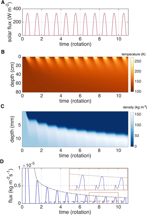
Figure 2. Evolution of insolation, subsurface temperature, water-frost content, and outgassing flux at the equator of comet 67P over 10 rotations.
Download figure:
Standard image High-resolution imageSeveral insights are gained from this preliminary result. The temperatures down to a shallow depth of about 20 cm were equilibrated quickly (panel (b)); after only three rotations or so, they exhibited a clear diurnal pattern, where the upper layers warmed up and cooled down before the layers underneath responded in kind. The diurnal fluctuations attenuated with depth and became indistinct below some 50 cm. The temperatures in deeper layers rose progressively as the heat penetrated and accumulated into the interiors.
At the beginning, the water ice retreated quickly when it was present in the upper layers where the highest temperatures occurred during daytime (panel (c)). As expected, an "apparent" ice front lowered at regular, (comet-)daily intervals. The ice seemed to be nearly stabilized at night. Meanwhile, the retreat slowed down visibly after several comet rotations, obviously because, after a dust mantle had built up, the ice became increasingly shielded from insolation and thereby experienced less intense sublimation. After 10 rotations, the ice front resided at a depth of some 7 mm. This is marginal to the mantle depth derived from the "thermal lag" of the subsurface, observed to sustain water activity for about an hour after sunset on 67P (Shi et al. 2016).
The evolution of the ice distribution in the subsurface is inherently connected with the variation of the outgassing (panel (d)). The peak outgassing flux decreased steadily over time, tracing a similar pattern to that of the ice "front." This epitomizes the insulating (and gas-resistant) effect(s) of the dust mantle that restricts the ice sublimation. A closer look at the outgassing curve reveals a secondary peak that became discernible after about five rotations (black dashed curve in the red rectangle). Unlike the primary peaks, the secondary gradually increased, albeit less notably, over time. Because the activities always occurred early in the day preceding the primary peak, we infer that they resulted from sublimation of nightly frost that had formed in the subsurface or, more specifically, in the dust mantle.
3. Formation of Diurnal Water Frost in the Subsurface
To confirm this interpretation, we focus on the results over the last (10th) body rotation in Figure 2. Figure 3 reexhibits the ice content in the top 10 mm below the surface but with a different color scale to reveal the minute variation. We observe a clear, diurnal formation of a frost layer whose density did not exceed 1 kg m−3 and is thus far lower than that at the ice front underneath (e.g., above 10 kg m−3). The frost disappeared during the day, concurrent with positive insolation, and so induced higher subsurface temperatures (panels (a) and (b)). As soon as insolation ceased, 3 the frost reappeared and quickly stabilized in like quantity. Figure 3(d) displays in higher spatial resolution the behavior of the ice front, initially located at about 7.2 mm but lowered visibly during the day.
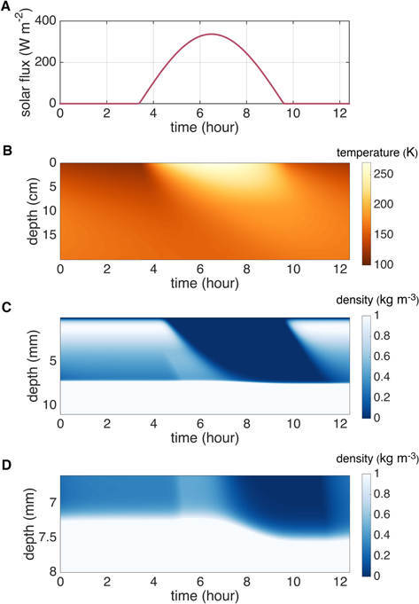
Figure 3. Diurnal insolation, temperature, and water-ice content in the subsurface at the equator of comet 67P.
Download figure:
Standard image High-resolution imageTwo things are worth noting. The peak of the frost density did not occur right at the surface but slightly underneath. This is because gas was assumed to diffuse outward directly into vacuum in the simulation, so that gas immediately below the surface escaped unhindered. Consequently, the frost formed most comfortably at a certain shallow depth, which was consistently less than 1 mm. The profile of the ice content will be discussed in more detail shortly. In Figures 3(c) and (d), the effect of a "backflow" is noticeable. The effect is reflected in an enhanced (slanted) column of frost that lies between the frost and ice fronts, beginning from slightly after 4 hr (about 5 hr in panel (d)) until the frost has completely depleted. It can be inferred that this enhancement was caused by frost sublimation; while part of the gas diffused upward before eventually escaping, the rest was transported inward and deposited, a phenomenon that is well known to result in the condensed ice "crust" (Prialnik & Mekler 1991).
3.1. Double Peaks in Ice Profile
It is instructive to examine more broadly the overall ice content as a function of depth. Figure 4(a) shows the profile of the ice density from the surface down to a depth of about 15 mm, after the ice profile had stabilized deep into the night. It is seen that the frost content was indeed quite insubstantial compared with the deeper, ice-rich layers, whose density reached over 150 kg m−3. Note that the initial ice density was 100 kg m−3; the excess then must have resulted from deposition of a backflow of water vapor. This region of enhanced density is reminiscent of the ice crust (Prialnik & Mekler 1991).
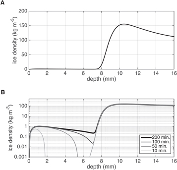
Figure 4. Characteristic profile of water-frost content in the subsurface and its evolution after local sunset at the equator of comet 67P.
Download figure:
Standard image High-resolution imageA better look at the plot is offered by rendering the density in logarithmic scale (Figure 4(b)). Here it is revealed that the profile consists of an additional peak for the frost, whose shape is analogous to that of the ice-rich layers underneath. Furthermore, when several profiles at intervals over time are shown, we may clearly trace the temporal development of the frost. The frost built up from shallow depths first and progressively pervaded lower layers. The process was completed at about 100 minutes after sunset (e.g., compared with the profile at 200 minutes).
Hence, the results suggest that the evolution of the frost layer is hardly distinct from that of the ice-rich layer in terms of mechanisms, apart from the difference in their abundances.
3.2. Consistency Check: Temporal Variation of Icy Fraction
Several tests were performed to check the consistency of our solutions, such as energy and mass conservation (Appendix B). One other test, in particular, turned out to be informative about the behavior of the frost. Figure 5(a) shows the same results as in Figure 3(c) but using a much coarser spatial discretization of Δx = xj+1 − xj = 1 mm. We see that the degradation of the spatial resolution did not cause significant errors in our solution. The pattern agrees well with that in Figure 3(c), albeit with a clear pixelated appearance. This agreement is confirmed by a comparison of the profiles for three resolutions of 1, 0.1, and 0.01 mm. Only the coarsest solution perceptibly deviates from the others; however, even in the worse case, the discrepancy is only in resolution, and no significant systematic deviation is present.
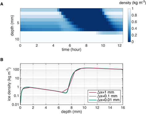
Figure 5. Impact of spatial resolution on the solution of subsurface frost content. (a) Same solution as in Figure 3(c) but with a depth increment of 1 mm instead of 0.01 mm. (b) Profiles of water-frost (ice) content solved with three spatial resolutions of 1, 0.1, and 0.01 mm, marked by red, black, and green lines, respectively.
Download figure:
Standard image High-resolution imageThe discrete pattern in Figure 5(a) accentuates the effect of the volumetric icy fraction (see Equation (9)), which characterizes the gradual decrease and accumulation of icy density in each layer. This phenomenon cannot be represented without the inclusion of the icy fraction. The omission of this factor is liable to inconsistency issues in the solution.
4. Morning Activity and "Nominal" Water Activity
Next, we reexamine the water outgassing flux as in Figure 2(d) over the last (10th) rotation. As noted, the flux crested shortly after 4 hr prior to the main peak (Figure 6(a)). When compared with the instantaneous subsurface gas density (Figure 6(b)), the first peak corresponds to the sublimation of the frost front (see the dash-lined slope in panel (b)). It is the very activity that drove the backflow of gas subsequently deposited, producing the concentrated frost in Figures 3(c) and (d) (also visible in Figure 5(a) in lower resolution).

Figure 6. Mass flux of water outgassing and gas density in the subsurface at the equator of comet 67P.
Download figure:
Standard image High-resolution imageThe ensuing primary activity corresponds to sublimation from the ice-rich layer, as evidenced by the highest gas density during the day. The depth of the highest gas density indeed seems to trace, or resulted effectively from, a sublimating ice front (nearly level, dashed line in Figure 6(b)). We note that the gas density exhibits a similar time-lag pattern to those of other states, such as temperature and ice density, expressed as a slant progression into deeper layers over time. After about 10 hr, the gas concentration had migrated inward; conceivably, such a flow (over several rotations) had contributed to enriching the ice layer underneath, e.g., producing the ice observed in Figure 4.
In Figure 7, the curves of outgassing flux for different heat conductivities and pore sizes are compared. The parameters strongly influence the behavior of water activity. As expected, with a tenfold higher conductivity of 0.02 W K−1 m−1, the outgassing intensified by a factor of about 3. The underamplification has been well noted in our previous studies. It reflects the mechanism of negative feedback; while heat conduction was 10 times more efficient, raising the interior temperature, part of the energy was consumed by stronger sublimation. As a result, the actual amplification of activity was always significantly smaller than 10. On the other hand, in a medium with smaller pores of 0.1 mm, the gas diffusion was more restricted. For instance, the flow resistance of a particulate medium is directly related to the number of particle layers (Gundlach et al. 2011). Hence, the smaller the particles or pores, the less efficient the gas diffusion through the medium. This is reflected in the reduction of the outgassing flux compared with the curve in the case of 1 mm sized pores. Due to negative feedback, we note that the reduction is less than 50%, once again, far less than a factor of 10, as in the case of increased conductivity.

Figure 7. Mass flux of water outgassing over one rotation of 67P for different heat conductivities and pore sizes. The units for conductivity are W K−1 m−1.
Download figure:
Standard image High-resolution imageIn every aspect, the morning activities shown here are the same as the regular morning outbursts presented by Prialnik et al. (2008), as the phenomena share the same mechanism. One difference seems to be in the relative magnitude of the frost sublimation. According to the results of Prialnik et al., the morning activities are stronger than the nominal activity. This can be easily explained by the much thicker mantle (of at least 3 cm) assumed in their model that quenched the activity. In our model, the mantle effect was much weaker and the daytime activity was sustained, as is compatible with the observed activity variation on 67P. On the other hand, both observations and the preliminary modeled results presented here indicate that the morning activity is an intrinsic component of the nominal diurnal activity. This is the case even in the absence of topography and thus without an abrupt change in illumination condition.
5. Effects of Adsorption and Nonzero Coma Density
5.1. Adsorption
The adsorption of water molecules was not considered in the results presented above. It has been well recognized that the density of the adsorbate may exceed the gas density in the pores (Schörghofer & Aharonson 2005). This condition is also observed in our simulations. As shown in Figure 8(a), the adsorbate water can reach the level of 10−5 kg m−3. The pattern is reminiscent of that of the gas density, as shown in Figure 6(b). The maximum corresponds to the highest gas density. Meanwhile, during daytime peak activity, the amount of adsorbate decreased steeply from maximum toward the surface. This deficiency corresponds to the dry layers where frost had already sublimated. These behaviors can be explained by the fact that adsorbate density increases with gas density but decreases with temperature (Schörghofer & Aharonson 2005). More specifically, in the shallow depths, above about 5 mm, the weak adsorption had resulted from a low gas density during the night but a high temperature during the day.

Figure 8. Absorbed water density in the subsurface and its impact on the ice density. (a) Evolution of absorbed density over a nucleus rotation. (b) Difference between ice densities in the presence or absence of adsorption. The black curve is for the case of millimeter-sized pores, while the gray curve is for 0.1 mm pores.
Download figure:
Standard image High-resolution imageThe impact of adsorption on the amount of frost formation is barely perceptible. The ice density profiles with and without adsorption are compared in Figure 8(b). The difference is orders of magnitude smaller than the ice density. This is understandable, since the adsorbate density itself, while larger than the gas density, is insignificant compared with the frost density on the order of 1 kg m−3. The difference in the case of smaller pores of 0.1 mm is greater by an order of magnitude (gray curve). The larger difference can be attributed to the fact that the adsorption is more effective in small pores, in which case the surface area, being inverse to the pore size, is larger (i.e., measured by the surface–volume ratio in Equations (7) and (10)). The peak adsorbate density is roughly an order of magnitude greater than that in the 1 mm pores but shares a similar pattern to that in Figure 8(a). The comparison of results illustrates that the impact of adsorption on frost formation should increase with its efficiency, i.e., with decreasing pore size.
5.2. Nonnegligible Gas Coma
It has been a common model assumption that gas diffuses into vacuum outside the nucleus, despite the fact that coma density may not be negligible, i.e., when the nucleus is active. The structure and evolution of the gas coma itself depend on the distribution of the outgassing flux and, essentially, the thermophysical and compositional properties of the nucleus subsurface. Rigorous characterization of the frost behavior would require simultaneous modeling of nucleus thermal behavior and the gas dynamics around it. While the task is beyond the scope of this study, it is instructive to examine in a simple case the impact of a nonzero, unvarying ambient density on frost formation in the nucleus subsurface.
Figure 9(a) and (b) compares the diurnal evolution of subsurface frost for ambient water densities of 10−10 and 10−9 kg m−3, respectively. With a higher density, more frost was accumulated immediately below the surface. Unlike the results in Figure 3, where it had formed and stabilized quickly after sunset, the frost here had continued to form throughout the night, as is clearly depicted in Figure 9(b) (less visibly so in panel (a)). The cause of this continuing enhancement is that outgoing gas could not escape (as easily as toward vacuum), and an inflow would even occur if the coma density was higher than the porous interior. The incoming gas was then deposited and enriched the frost reservoir starting from the shallow subsurface. Figure 9(c) comparatively shows the ice density profiles for the different coma densities at about 4 hr, i.e., deep into the night. As has been noted (Figure 4(b)), in the absence of a coma, the frost could not form in the outermost layers, as gas would escape rather than be deposited. When the coma had a density of 10−10 kg m−3, the outward diffusion became restricted, and frost could accumulate close to the surface (dark blue curve). For an even denser coma of 10−9 kg m−3, the significant and sustained nightly inflow caused an enhancement noticeable down to a greater depth of 2 mm (light blue curve). The steep profile gradient toward the surface indicates that the frost enhancement would have occurred in progressively deeper layers as well, if time had permitted.
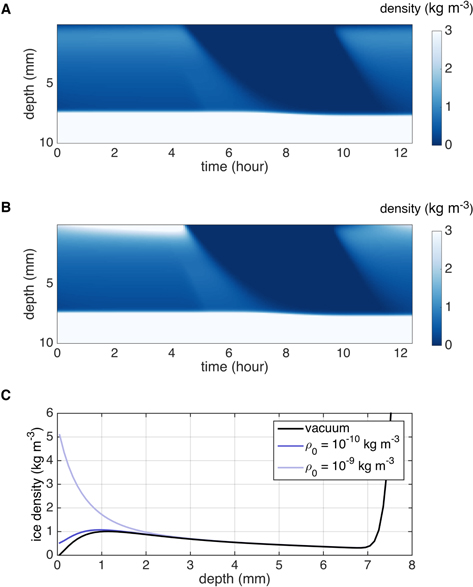
Figure 9. Diurnal evolution of water-frost density in the subsurface in the cases of nonzero ambient gas density. (a) Frost density in the case of an ambient gas density of ρ0 = 10−10 kg m−3. (b) Same as panel (a) but for ρ0 = 10−9 kg m−3. (c) Comparison of three ice density profiles for the vacuum case and those of nonnegligible coma densities.
Download figure:
Standard image High-resolution image6. Conclusion and Discussion
The main conclusions of this model investigation can be summarized as follows.
- 1.Water frost forms prevalently near the uppermost surface layers of 67P during the night. The condition of its occurrence is hardly restrictive. Most notably, the phenomenon does not rely on topographic irregularity whatsoever. The formation process is analogous to that of the condensed ice-rich layer underneath.
- 2.The nightly frost sublimates early in the morning and depletes quickly, often producing a discernible peak of outgassing flux. The dust mantle on 67P does not exceed the diurnal skin depth, and the water outgassing displays a distinct diurnal variation. The frost sublimation could amount to some tenths of the daily maximum flux. With a thick enough mantle, the frost activity may surpass that from underneath, as is the case of Tempel 1 (Prialnik et al. 2008). In either case, frost activity represents a regular, nominal component of the diurnal water outgassing.
- 3.The role of water adsorption is considered in the present analysis. For 67P, assumed to consist of large particles or pores, e.g., larger than 0.1 mm, the adsorption plays an insignificant role. However, this effect will increase in smaller pores.
As an aside, several aspects of water activity revealed in this analysis echoed our earlier findings based on a simplified thermal model assuming a constant dust mantle (Hu et al. 2017b). For example, the presence of the mantle strongly regulates the outgassing flux, and the heat consumed by activity is, in fact, marginal (see Appendix B). The effect of the thermal lag is evident (Figure 10; see also Shi et al. 2016). For evaluating the global activity behavior of 67P, such as its total gas production rate, the application of the dust mantle model should be acceptable with a reasonable parameterization.
Various details are left to be addressed by future studies. The amount of frost typically redistributed over a diurnal cycle in our model calculations seems to be scantier than the Rosetta observations by an order of magnitude. There could be several explanations. For example, while not required, topography may still play an important role in affecting the frost abundance. In addition, the influence of the gas coma may not be negligible, an investigation of which is underway.
We thank two reviewers for providing constructive criticism that led to an improved manuscript. The authors thank Dr. Holger Sierks and Dr. Carsten Güttler for many discussions concerning the analysis and interpretation of the Rosetta/OSIRIS imaging data. The authors express their gratitude to Dr. Ekkehard Kührt for stimulating discussions that facilitated this study. X.H. appreciates discussions with Dr. Philipp Gläser about stepwise iterations that offered a solution to the encountered problem of diffusion/deposition ambiguity.
Appendix A: Partial Derivatives of Adsorption Density
The partial derivatives in Equation (10) for the adsorbed density are


with shorthand

where P is the gas pressure according to the ideal gas law. The expression of Equation (A1) incurs a singularity in case ρg = 0. For this reason, the initial values of the gas density were set to the saturation level, ρV g, in the simulation, in which case the change rate of adsorption depends solely on temperature (and its change rate), namely,

Appendix B: Heat Budget and Mass Loss
The tests of the energy conservation and mass balance are briefly presented here for the diurnal case. In the former, we examined three quantities. First, the heat flux of thermal emission is  in Equation (17). Second, the heat loss via water outgassing is cg
Zg
T(0) + ℓg
ζg(0) (g = 1) in the same expression; note that the second component of surface sublimation is practically always zero. Third, the internal energy is given by the integral
in Equation (17). Second, the heat loss via water outgassing is cg
Zg
T(0) + ℓg
ζg(0) (g = 1) in the same expression; note that the second component of surface sublimation is practically always zero. Third, the internal energy is given by the integral  , where U(x) = c
ρ(x)T(x). The sum of the three quantities is theoretically equal to the flux of the energy input. Figure 10 shows the diurnal variation of the quantities together with the energy input of insolation. It is observed that most of the heat was emitted via thermal radiation. On the other hand, the energy loss due to outgassing was insignificant, in this case, less than 1% of the maximum insolation. The heat balance, here indicative of our numerical errors, reached 0.4 W m−2 at maximum, amounting to about 0.1% of the total heat. We note that, while comparable to the heat consumption of outgassing, this error is accumulated over all depths and does not indicate an absolute uncertainty in the outgassing flux or mass balance (or ice loss).
, where U(x) = c
ρ(x)T(x). The sum of the three quantities is theoretically equal to the flux of the energy input. Figure 10 shows the diurnal variation of the quantities together with the energy input of insolation. It is observed that most of the heat was emitted via thermal radiation. On the other hand, the energy loss due to outgassing was insignificant, in this case, less than 1% of the maximum insolation. The heat balance, here indicative of our numerical errors, reached 0.4 W m−2 at maximum, amounting to about 0.1% of the total heat. We note that, while comparable to the heat consumption of outgassing, this error is accumulated over all depths and does not indicate an absolute uncertainty in the outgassing flux or mass balance (or ice loss).
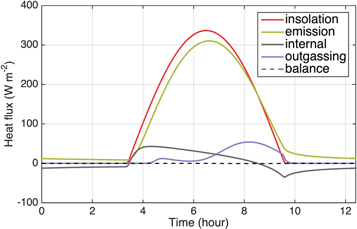
Figure 10. Energy budget of the system over a comet rotation. Note that heat loss by outgassing is magnified by a factor of 100 for the purpose of comparison.
Download figure:
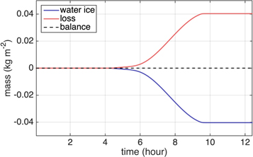
Standard image High-resolution imageTo test the mass balance, we derived the accumulated water-ice loss due to outgassing. In Figure 11, the ice loss is compared with the remainder of the ice mass in the subsurface. For the purpose of comparison, the latter is calibrated by subtracting the initial total mass. In the ideal case, the two should be of opposite signs; in reality, their sum is a measure of numerical errors. Here the maximum is 2 × 10⁻⁶ kg m−2, indicating an error on the level of 0.1% commensurate with that for energy balance (Figure 10).
Figure 11. Water-ice loss over a comet rotation compared with the remainder mass.
Download figure:
Standard image High-resolution image
Footnotes
- 3
More specifically, the frost started to form shortly before dark, when the surface had already cooled down with vanishing insolation at dusk. Note that, because no topographic obstruction is considered, the attenuation of insolation is gradual.