


Abstract
We present X-SHOOTER near-IR spectroscopy of a large sample of 38 luminous (M1450 = −29.0 to −24.4) quasars at 5.78 < z < 7.54, which have complementary [C ii]158μm observations from ALMA. This X-SHOOTER/ALMA sample provides us with the most comprehensive view of reionization-era quasars to date, allowing us to connect the quasar properties with those of its host galaxy. In this work we introduce the sample, discuss data reduction and spectral fitting, and present an analysis of the broad emission line properties. The measured Fe ii/Mg ii flux ratio suggests that the broad-line regions of all quasars in the sample are already enriched in iron. We also find the Mg ii line to be on average blueshifted with respect to the [C ii] redshift with a median of −391 km s−1. A significant correlation between the Mg ii−[C ii]158μm and C iv−[C ii]158μm velocity shifts indicates a common physical origin. Furthermore, we fRequently detect large C iv–Mg ii emission line velocity blueshifts in our sample with a median value of −1848 km s−1. While we find all other broad emission line properties not to be evolving with redshift, the median C iv–Mg ii blueshift is much larger than found in low-redshift, luminosity-matched quasars (−800 km s−1). Dividing our sample into two redshift bins, we confirm an increase of the average C iv–Mg ii blueshift with increasing redshift. Future observations of the rest-frame optical spectrum with the James Webb Space Telescope will be instrumental in further constraining the possible evolution of quasar properties in the epoch of reionization.
Export citation and abstract BibTeX RIS
1. Introduction
Quasars are the most luminous nontransient light sources in the universe. They are galaxies in which mass accretion onto a supermassive black hole (SMBH) dominates UV and optical emission, and they can be discovered well into the epoch of reionization (z > 6; Fan et al. 2006). In this last major phase transition of the universe, neutral hydrogen is being ionized by UV emission of the first generation of galaxies and accreting SMBHs. High-redshift quasars at z > 6 not only provide a window into the formation and early growth of SMBHs but also facilitate the study of massive high-redshift galaxy evolution, probe the onset of BH host galaxy coevolution, and shed light on the process of reionization.
The advent of wide-area photometric surveys has increased the number of known quasars at z > 6 to ∼200 by today (e.g., Fan et al. 2001; Bañados et al. 2016; Matsuoka et al. 2019a; Reed et al. 2019; Yang et al. 2019; Wang et al. 2019). Above z = 7 only seven quasars are known to date (Mortlock et al. 2011; Wang et al. 2018; Matsuoka et al. 2018, 2019b; Yang et al. 2019, 2020), with ULAS J1342+0928 at z = 7.54 (Bañados et al. 2018) being the most distant quasar known.
Rest-frame UV and optical spectra of quasars have been key to identifying the origin of the emission as mass accretion onto an SMBH (Lynden-Bell 1969). We now understand that the broad emission lines (FWHM ≳ 1000 km s−1) seen in the spectra originate from mostly virialized gas orbiting the central SMBH at subparsec scales, the so-called broad-line region (BLR). Narrow emission lines (FWHM ≲ 500 km s−1) often seen in addition to the broad lines emanate from gas at kiloparsec scales, known as the narrow-line region (NLR). The kinematics of the BLR imprinted on the broad emission lines allow us to estimate the SMBH mass and further understand the dynamics of the accretion process (Peterson 1993; Peterson et al. 2004).
At z > 6 the rest-frame UV spectrum is shifted into the optical/near-IR (NIR) wavelength range, and the region blueward of 1216 Å, including parts of the the Lyα line, is strongly absorbed by the intergalactic medium owing to the resonant nature of Lyα photons in neutral hydrogen (e.g., Michel-Dansac et al. 2020). Therefore, NIR spectroscopy is necessary to fully characterize the quasar's spectrum and exploit the information provided by the broad and narrow emission lines. Many high-redshift quasars have thus been followed up either individually or in small (N < 10) samples (e.g., Jiang et al. 2007; Kurk et al. 2007; De Rosa et al. 2014; Onoue et al. 2019). However, the discovery of hundreds of quasars above z ≈ 6 has paved the way for studies of increasingly larger samples (De Rosa et al. 2011; Mazzucchelli et al. 2017; Becker et al. 2019), enabling first insights into the population properties of high-redshift quasars. The largest study at z ≳ 5.7 to date (Shen et al. 2019b) presents NIR spectra and measured properties for a total of 50 quasars.
Studies of z > 6 quasars have revealed large SMBH masses, ∼108–1010 M⊙ (e.g., Wu et al. 2015; Onoue et al. 2019), only 1 Gyr after the big bang, setting strong constraints on models of BH formation and evolution (for a review see Volonteri 2012). The majority of z > 6 quasars are found to have high accretion rates as characterized by their high Eddington luminosity ratios of Lbol/LEdd ≥ 0.1. Interestingly, general properties (spectral shape, maximum SMBH mass, BLR metallicity, Fe ii/Mg ii flux ratio) of quasars at z > 6 show no or only a weak evolution with redshift (e.g., Jiang et al. 2007; De Rosa et al. 2011, 2014; Mazzucchelli et al. 2017; Shen et al. 2019b). The only exception seems to be the C iv–Mg ii velocity shift. It was already known that a large fraction of z ≳ 6 quasars exhibit highly blueshifted C iv emission compared to their Mg ii redshift (e.g., De Rosa et al. 2014; Mazzucchelli et al. 2017; Reed et al. 2019), indicative of an outflowing component in the C iv emission line (e.g., Gaskell 1982). A comparison across (luminosity-matched) quasar samples at different redshifts (Meyer et al. 2019) has highlighted that large C iv blueshifts are much more common in z > 6.5 quasars than at lower redshifts.
On the other hand, it is currently unclear whether this evolution is an intrinsic change or induced by selection effects. Quasars at z > 6 are predominantly selected by the strong Lyα break in their spectrum. In addition, available photometry limits z > 6 quasar searches to the bright end (M1450 ≤ −25.5) of the quasar distribution (Wang et al. 2019). Only the Canada-France High-z Quasar Survey (Willott et al. 2010) and the recent efforts of the Subaru High-z Exploration of Low-luminosity Quasars (SHELLQs) project (e.g., Matsuoka et al. 2016, 2019a) have provided a first look at the fainter z > 6 quasar population. These lower-luminosity quasars show on average less massive SMBHs (∼107–109 M⊙; e.g., Willott et al. 2017; Onoue et al. 2019) compared to their luminous counterparts. Unfortunately, only a handful of NIR spectroscopic measurements exist to date for low-luminosity z > 6 quasars.
Investigations of high-redshift quasars are often complemented with studies of the host galaxy gas via rotational transitions of the carbon monoxide (CO) molecule or the fine-structure line of singly ionized carbon [C ii] at 158 μm, which enters the 1.2 mm atmospheric window for quasars at z ≳ 6. Millimeter observations so far provide the only direct probes for the host galaxy in high-redshift quasars. As the [C ii] line is the main coolant of the cool (<1000 K) interstellar material, it is a very bright line easily detectable at cosmological distances. The [C ii] line and the underlying far-IR (FIR) dust continuum emission allow measurements of precise [C ii] redshifts, estimates of the dynamical masses, and star formation rates. Since the first [C ii] line detection at z > 0.1 in the host galaxy of J1148+5251, a quasar at z = 6.4 (Maiolino et al. 2005), the [C ii] line has become a widely used diagnostic for high-redshift quasar hosts (e.g., Walter et al. 2009; Venemans et al. 2012; Wang et al. 2013; Willott et al. 2013, 2015; Bañados et al. 2015; Venemans et al. 2016; Mazzucchelli et al. 2017; Izumi et al. 2018, 2019; Eilers et al. 2020; Venemans et al. 2020).
We here present the analysis of the NIR spectra of 38 quasars, capitalizing on new and archival VLT/X-SHOOTER data. All quasars in our sample have also been targeted and observed at millimeter wavelengths to detect the [C ii] emission. Successful detection of 34 of our 38 quasars (Decarli et al. 2018; Eilers et al. 2020; Venemans et al. 2020) thus complements our sample with precise systemic redshifts and additional information on the cold interstellar medium (ISM) and dust emission of the host galaxy. The combined information on the quasar and its host provides us with a comprehensive view on the full quasar phenomenon, unique to the X-SHOOTER/ALMA sample. In this paper we present the X-SHOOTER NIR spectral analysis of the quasar sample and an in-depth discussion of the quasars' rest-frame UV properties. A companion paper (E. P. Farina et al. 2020, in preparation) will present the SMBH masses and discuss them in context with their host galaxies. That paper will also put the sample in context with VLT/MUSE observations (REQUIEM; Farina et al. 2019), which probe the immediate environment in Lyα emission (see also Drake et al. 2019). Data reduction of the optical quasar spectra taken by the X-SHOOTER visual arm (VIS) is ongoing and will be presented in a future publication.
In Section 2 we give an overview of the quasar sample and describe the data reduction. We lay out our spectral fitting methodology in detail in Section 3 and describe the analysis of the fits in Section 4. Section 5 is devoted to a discussion on the biases inherent in adopting different iron pseudocontinuum templates. We analyze the iron enrichment of the BLR in Section 6.1 and examine the properties of the broad C iv and Mg ii lines in Section 6.2. Our findings are summarized in Section 7.
Throughout this work we adopt a standard flat ΛCDM cosmology with H0 = 70 km s−1 Mpc−1, ΩM = 0.3, and ΩΛ = 0.7 in broad agreement with the results of the Planck mission (Planck Collaboration et al. 2016). All magnitudes are reported in the AB photometric system.
2. The X-SHOOTER/ALMA Sample
The sample we present herein consists of 38 quasars with redshifts between z = 5.78 and z = 7.54 (median z = 6.18). They were selected to have both NIR X-SHOOTER spectroscopy and ALMA millimeter observations of the quasar host. The millimeter observations are crucial, as they allow us to place the quasar (BH mass, Eddington ratio, line redshifts, etc.) in context with the galaxy (systemic redshift, dynamical mass, gas mass, etc.). While the millimeter ALMA results have been previously published (Venemans et al. 2017; Decarli et al. 2018; Bañados et al. 2019a; Venemans et al. 2019, 2020; Eilers et al. 2020), a large fraction of the X-SHOOTER spectroscopy is presented here for the first time. An overview of the sample is given in Tables 1 and 2.
Table 1. X-SHOOTER/ALMA Sample of High-redshift Quasars—General Quasar Properties
| Quasar Name | R.A. (J2000) | Decl. (J2000) | zsys | Method | Reference | Cross | Modeled Lines | J Band |
|---|---|---|---|---|---|---|---|---|
| (hh:mm:ss.sss) | (dd:mm:ss.ss) | (zsys) | (zsys) | Reference | (AB mag) | |||
| PSO J004.3936+17.0862 | 00:17:34.467 | +17:05:10.70 | 5.8165 ± 0.0023 | [Cii] | Eilers et al. (2020) | g | C iv(1G), C III], Mg ii | 20.67 ± 0.16 |
| PSO J007.0273+04.9571 | 00:28:06.560 | +04:57:25.68 | 6.0015 ± 0.0002 | [Cii] | Venemans et al. (2020) | f | C iv, C III], Mg ii | 19.77 ± 0.11 |
| PSO J009.7355–10.4316 | 00:38:56.522 | −10:25:53.90 | 6.0040 ± 0.0003 | [Cii] | Venemans et al. (2020) | C iv(1G) | 19.93 ± 0.07 | |
| PSO J011.3898+09.0324 | 00:45:33.568 | +09:01:56.96 | 6.4694 ± 0.0025 | [Cii] | Eilers et al. (2020) | g | C iv(1G), Mg ii | 20.80 ± 0.13 |
| VIK J0046–2837 | 00:46:23.645 | −28:37:47.34 | 5.9926 ± 0.0028 | Mgii | This work | Mg ii | 20.96 ± 0.09 | |
| SDSS J0100+2802 | 01:00:13.027 | +28:02:25.84 | 6.3269 ± 0.0002 | [Cii] | Venemans et al. (2020) | e | Mg ii | 17.64 ± 0.02 |
| VIK J0109–3047 | 01:09:53.131 | −30:47:26.31 | 6.7904 ± 0.0003 | [Cii] | Venemans et al. (2020) | b,c,e | C iv(1G), Mg ii | 21.27 ± 0.16 |
| PSO J036.5078+03.0498 | 02:26:01.875 | +03:02:59.40 | 6.5405 ± 0.0001 | [Cii] | Venemans et al. (2020) | c,e | Si iv, C iv(1G), Mg ii | 19.51 ± 0.03 |
| VIK J0305–3150 | 03:05:16.916 | −31:50:55.90 | 6.6139 ± 0.0001 | [Cii] | Venemans et al. (2019) | b,c,e | C iv(1G), Mg ii | 20.68 ± 0.07 |
| PSO J056.7168–16.4769 | 03:46:52.044 | −16:28:36.88 | 5.9670 ± 0.0023 | [Cii] | Eilers et al. (2020) | g | C iv, C III], Mg ii | 20.25 ± 0.10 |
| PSO J065.4085–26.9543 | 04:21:38.049 | −26:57:15.61 | 6.1871 ± 0.0003 | [Cii] | Venemans et al. (2020) | C iv(1G), Mg ii | 19.36 ± 0.02 | |
| PSO J065.5041–19.4579 | 04:22:00.995 | −19:27:28.69 | 6.1247 ± 0.0006 | [Cii] | Decarli et al. (2018) | C iv(1G), Mg ii | 19.90 ± 0.15 | |
| SDSS J0842+1218 | 08:42:29.430 | +12:18:50.50 | 6.0754 ± 0.0005 | [Cii] | Venemans et al. (2020) | a,f | C iv, Mg ii | 19.78 ± 0.03 |
| SDSS J1030+0524 | 10:30:27.098 | +05:24:55.00 | 6.3048 ± 0.0012 | LyaH | Farina et al. (2019) | a,e | C iv, Mg ii | 19.79 ± 0.08 |
| PSO J158.69378–14.42107 | 10:34:46.509 | −14:25:15.89 | 6.0681 ± 0.0024 | [Cii] | Eilers et al. (2020) | g | C iv, Mg ii | 19.19 ± 0.06 |
| PSO J159.2257–02.5438 | 10:36:54.190 | −02:32:37.94 | 6.3809 ± 0.0005 | [Cii] | Decarli et al. (2018) | C iv, Mg ii | 20.00 ± 0.10 | |
| SDSS J1044–0125 | 10:44:33.041 | −01:25:02.20 | 5.7846 ± 0.0005 | [Cii] | Venemans et al. (2020) | e,f | C iv(1G), C III] | 19.25 ± 0.05 |
| VIK J1048–0109 | 10:48:19.082 | −01:09:40.29 | 6.6759 ± 0.0002 | [Cii] | Venemans et al. (2020) | Mg ii | 20.65 ± 0.17 | |
| ULAS J1120+0641 | 11:20:01.478 | +06:41:24.30 | 7.0848 ± 0.0004 | [Cii] | Venemans et al. (2020) | b,c,e | Si iv, C iv, C III] | 20.36 ± 0.05 |
| ULAS J1148+0702 | 11:48:03.286 | +07:02:08.33 | 6.3337 ± 0.0028 | Mgii | This work | f | C iv, Mg ii | 20.30 ± 0.11 |
| PSO J183.1124+05.0926 | 12:12:26.984 | +05:05:33.49 | 6.4386 ± 0.0002 | [Cii] | Venemans et al. (2020) | e | C iv(1G), Mg ii | 19.77 ± 0.08 |
| SDSS J1306+0356 | 13:06:08.258 | +03:56:26.30 | 6.0330 ± 0.0002 | [Cii] | Venemans et al. (2020) | a,e | C iv, C III], Mg ii | 19.71 ± 0.10 |
| ULAS J1319+0950 | 13:19:11.302 | +09:50:51.49 | 6.1347 ± 0.0005 | [Cii] | Venemans et al. (2020) | e | C iv, C III], Mg ii | 19.70 ± 0.03 |
| ULAS J1342+0928 | 13:42:08.105 | +09:28:38.61 | 7.5400 ± 0.0003 | [Cii] | Bañados et al. (2019a) | e | Si iv, C iv(1G), C III] | 20.30 ± 0.02 |
| CFHQS J1509–1749 | 15:09:41.779 | −17:49:26.80 | 6.1225 ± 0.0007 | [Cii] | Decarli et al. (2018) | e | C iv, C III], Mg ii | 19.80 ± 0.08 |
| PSO J231.6576–20.8335 | 15:26:37.838 | −20:50:00.66 | 6.5869 ± 0.0004 | [Cii] | Venemans et al. (2020) | c,e | Mg ii | 19.66 ± 0.05 |
| PSO J239.7124–07.4026 | 15:58:50.991 | −07:24:09.59 | 6.1097 ± 0.0024 | [Cii] | Eilers et al. (2020) | g | C iv, Mg ii | 19.35 ± 0.08 |
| PSO J308.0416–21.2339 | 20:32:09.994 | −21:14:02.31 | 6.2355 ± 0.0003 | [Cii] | Venemans et al. (2020) | C iv, Mg ii | 20.17 ± 0.11 | |
| SDSS J2054–0005 | 20:54:06.490 | −00:05:14.80 | 6.0389 ± 0.0001 | [Cii] | Venemans et al. (2020) | C iv(1G), C III], Mg ii | 20.12 ± 0.06 | |
| CFHQS J2100–1715 | 21:00:54.619 | −17:15:22.50 | 6.0807 ± 0.0004 | [Cii] | Venemans et al. (2020) | g | C iv(1G), Mg ii | 21.42 ± 0.10 |
| PSO J323.1382+12.2986 | 21:32:33.189 | +12:17:55.26 | 6.5872 ± 0.0004 | [Cii] | Venemans et al. (2020) | c,e | Si iv, C iv, C III], Mg ii | 19.74 ± 0.03 |
| VIK J2211–3206 | 22:11:12.391 | −32:06:12.95 | 6.3394 ± 0.0010 | [Cii] | Decarli et al. (2018) | C iv(1G), Mg ii | 19.62 ± 0.03 | |
| CFHQS J2229+1457 | 22:29:01.649 | +14:57:09.00 | 6.1517 ± 0.0005 | [Cii] | Willott et al. (2015) | g | C iv | 21.95 ± 0.07 |
| PSO J340.2041–18.6621 | 22:40:49.001 | −18:39:43.81 | 6.0007 ± 0.0020 | LyaH | Farina et al. (2019) | C iv, C III],Mg ii | 20.28 ± 0.08 | |
| SDSS J2310+1855 | 23:10:38.880 | +18:55:19.70 | 6.0031 ± 0.0002 | [Cii] | Wang et al. (2013) | f | C iv(1G), Mg ii | 18.88 ± 0.05 |
| VIK J2318–3029 | 23:18:33.103 | −30:29:33.36 | 6.1456 ± 0.0002 | [Cii] | Venemans et al. (2020) | C iv(1G), Mg ii | 20.20 ± 0.06 | |
| VIK J2348–3054 | 23:48:33.336 | −30:54:10.24 | 6.9007 ± 0.0005 | [Cii] | Venemans et al. (2020) | b,c,e | C iv(1G), C III], Mg ii | 21.14 ± 0.08 |
| PSO J359.1352–06.3831 | 23:56:32.452 | −06:22:59.26 | 6.1719 ± 0.0002 | [Cii] | Venemans et al. (2020) | g | C iv(1G), Mg ii | 19.85 ± 0.10 |
Note. Quasar coordinates are available in decimal degrees in an online table summarized in Table 9. Redshift method abbreviations: [Cii]—peak of the [C ii]158μm line; Mgii—peak of the Mgii λ2798 line; LyaH—determined from the Lyα halo.
References. The cross-references in the table denote previous publications analyzing NIR spectroscopy of these quasars. The references are: a = De Rosa et al. (2011), b = De Rosa et al. (2014), c = Mazzucchelli et al. (2017), d = Onoue et al. (2019), e = Meyer et al. (2019), f = Shen et al. (2019b), g = Eilers et al. (2020).
Download table as: ASCIITypeset image
Table 2. X-SHOOTER/ALMA Sample of High-redshift Quasars—Information on X-SHOOTER Spectroscopy and Discovery Reference
| Quasar Name | Exp. Time (s) | X-SHOOTER Proposal ID | PI | Discovery Ref. |
|---|---|---|---|---|
| PSO J004.3936+17.0862 | 3600 | 0101.B-0272(A) | Eilers | Bañados et al. (2016) |
| PSO J007.0273+04.9571 | 2400 | 098.B-0537(A) | Farina | Bañados et al. (2014); Jiang et al. (2015) |
| PSO J009.7355–10.4316 | 4800 | 097.B-1070(A) | Farina | Bañados et al. (2016) |
| PSO J011.3898+09.0324 | 3600 | 0101.B-0272(A) | Eilers | Mazzucchelli et al. (2017) |
| VIK J0046–2837 | 12000 | 097.B-1070(A) | Farina | Decarli et al. (2018) |
| SDSS J0100+2802 | 10800 | 096.A-0095(A) | Pettini | Wu et al. (2015) |
| VIK J0109–3047 | 24000 | 087.A-0890(A), 088.A-0897(A) | De Rosa, De Rosa | Venemans et al. (2013) |
| PSO J036.5078+03.0498 | 14400 | 0100.A-0625(A), 0102.A-0154(A) | D'Odorico, D'Odorico | Venemans et al. (2015) |
| VIK J0305–3150 | 16800 | 098.B-0537(A) | Farina | Venemans et al. (2013) |
| PSO J056.7168–16.4769 | 7200 | 097.B-1070(A) | Farina | Bañados et al. (2016) |
| PSO J065.4085–26.9543 | 2400 | 098.B-0537(A) | Farina | Bañados et al. (2016) |
| PSO J065.5041–19.4579 | 4800 | 097.B-1070(A) | Farina | Bañados et al. (2016) |
| SDSS J0842+1218 | 7200 | 097.B-1070(A) | Farina | De Rosa et al. (2011); Jiang et al. (2015) |
| SDSS J1030+0524 | 4800 | 086.A-0162(A) | D'Odorico | Fan et al. (2001) |
| PSO J158.69378–14.42107 | 4320 | 096.A-0418(B) | Shanks | Chehade et al. (2018) |
| PSO J159.2257–02.5438 | 4800 | 098.B-0537(A) | Farina | Bañados et al. (2016) |
| SDSS J1044–0125 | 2400 | 084.A-0360(A) | Hjorth | Fan et al. (2000) |
| VIK J1048–0109 | 4800 | 097.B-1070(A) | Farina | Wang et al. (2017) |
| ULAS J1120+0641 | 72000 | 286.A-5025(A), 089.A-0814(A), 093.A-0707(A) | Venemans, Becker, Becker | Mortlock et al. (2011) |
| ULAS J1148+0702 | 9600 | 098.B-0537(A) | Farina | Jiang et al. (2016) |
| PSO J183.1124+05.0926 | 4800 | 098.B-0537(A) | Farina | Mazzucchelli et al. (2017) |
| SDSS J1306+0356 | 41400 | 084.A-0390(A) | Ryan-Weber | Fan et al. (2001) |
| ULAS J1319+0950 | 36000 | 084.A-0390(A) | Ryan-Weber | Mortlock et al. (2009) |
| ULAS J1342+0928 | 80400 | 098.B-0537(A), 0100.A-0898(A) | Farina, Venemans | Bañados et al. (2018) |
| CFHQS J1509–1749 | 24000 | 085.A-0299(A), 091.C-0934(B) | D'Odorico, Kaper | Willott et al. (2007) |
| PSO J231.6576–20.8335 | 2400 | 097.B-1070(A) | Farina | Mazzucchelli et al. (2017) |
| PSO J239.7124–07.4026 | 3600 | 0101.B-0272(A) | Eilers | Bañados et al. (2016) |
| PSO J308.0416–21.2339 | 9600 | 098.B-0537(A) | Farina | Bañados et al. (2016) |
| SDSS J2054–0005 | 7200 | 60.A-9418(A) | Ryan-Weber | Jiang et al. (2008) |
| CFHQS J2100–1715 | 12000 | 097.B-1070(A) | Farina | Willott et al. (2010) |
| PSO J323.1382+12.2986 | 7200 | 098.B-0537(A) | Farina | Mazzucchelli et al. (2017) |
| VIK J2211–3206 | 5280 | 096.A-0418(A), 098.B-0537(A) | Shanks, Farina | Decarli et al. (2018) |
| CFHQS J2229+1457 | 6000 | 0101.B-0272(A) | Eilers | Willott et al. (2010) |
| PSO J340.2041–18.6621 | 9600 | 098.B-0537(A) | Farina | Bañados et al. (2014) |
| SDSS J2310+1855 | 2400 | 098.B-0537(A) | Farina | Wang et al. (2013); Jiang et al. (2016) |
| VIK J2318–3029 | 9600 | 097.B-1070(A) | Farina | Decarli et al. (2018) |
| VIK J2348–3054 | 9200 | 087.A-0890(A) | De Rosa | Venemans et al. (2013) |
| PSO J359.1352–06.3831 | 4800 | 098.B-0537(A) | Farina | Bañados et al. (2016); Wang et al. (2016a) |
Download table as: ASCIITypeset image
With the exception of four sources, we adopt systemic redshifts measured from the [C ii]158μm emission line. As shown in Figure 4 of Decarli et al. (2018), the [C ii]158μm-based redshifts provide a substantial improvement over the quasar discovery redshifts. Their comparison includes a large fraction of our sample.
Figure 1 shows the X-SHOOTER/ALMA sample in the plane of bolometric luminosity and redshift, compared to other samples with NIR spectroscopy from the literature. The quasars in our sample can be considered luminous with a median absolute magnitude of M1450 = −26.5 (−29.0 to −24.4), as determined from their spectral fits. With the exception of SDSS J0100+2802 ( ), all other quasars lie in a narrow range of bolometric luminosities,
  to 47.67 (median 47.26). Details on how the bolometric luminosity was calculated from the spectra are provided in Section 4.

Figure 1. Quasars at z > 5.5 with available NIR spectroscopy as a function of their bolometric luminosity and redshift. Quasars of this study are highlighted as orange circles. Filled orange circles refer to objects with successful continuum fits, whereas open orange circles refer to the five objects where we could not fit the continuum shape with a power law. Quasars from other studies are represented with blue and green symbols according to the legend.
Download figure:
Standard image High-resolution imageThe recently published compilation of 50 quasars with GNIRS spectroscopy (Shen et al. 2019b) is shown as blue diamonds in Figure 1. Compared to our work, their quasar sample is at slightly lower redshifts (median z = 5.97) and on average less luminous (median  ).
).
2.1. The X-SHOOTER Spectroscopy
The X-SHOOTER spectrograph (Vernet et al. 2011) covers the wavelength range from 300 to 2500 nm with three spectral arms (UVB: 300–559.5 nm; VIS: 559.5–1024 nm; NIR: 1024–2480 nm). By design the spectral format for the three arms is fixed, resulting in the same wavelength coverage for all observations.
For the purpose of this work we focus on the NIR spectroscopy to study the broad Si iv, C iv, C iii], and Mg ii quasar emission lines. The X-SHOOTER NIR spectroscopy of our sample was collected from a variety of observing programs listed in Table 2. Total exposure times of the NIR observations vary between 2400 and 80,400 s (median 7200 s). The observations were taken with slit widths of 0 6, 09, and 12, resulting in resolutions of R ∼ 8100, ∼5600, and ∼4300, respectively, for the NIR arm.
2.2. Data Reduction of the X-SHOOTER Near-infrared Spectroscopy
In order to guarantee a homogeneous analysis, we reduce the X-SHOOTER NIR spectra using the newly developed open-source Python Spectroscopic Data Reduction Pipeline, PypeIt13 (Prochaska et al. 2019, 2020). We include six quasar spectra in our sample, which were already reduced with PypeIt and presented in Eilers et al. (2020). The pipeline uses supplied flat-field images to automatically trace the echelle orders and correct for the detector illumination. Difference imaging of dithered AB pairs and a 2D BSpline fitting procedure are used to perform sky subtraction on the 2D images. Object traces are automatically identified and extracted to produce 1D spectra using the optimal spectrum extraction technique (Horne 1986). We apply a relative flux correction to all 1D spectra using X-SHOOTER flux standards, which were taken at most 6 months apart from the observations. All flux-calibrated 1D spectra of each quasar are then co-added and corrected for telluric absorption using PypeIt. A telluric model is fit to correct the absorbed science spectrum up to a best-fit PCA model (Davies et al. 2018) of said spectrum. The telluric model is based on telluric model grids produced from the Line-By-Line Radiative Transfer Model (LBLRTM4; Clough et al. 2005; Gullikson et al. 2014). In the last step we apply an absolute flux calibration to the fully reduced quasar spectra. All quasars in our sample have available J-band photometry measurements in the literature, while only a subset has K-band measurements. Therefore, we normalized the spectra using the J-band magnitudes (see Table 1). The NIR quasar spectra were not corrected for Galactic extinction, which is negligible at the observed wavelengths.
2.3. Properties of the X-SHOOTER/ALMA Sample
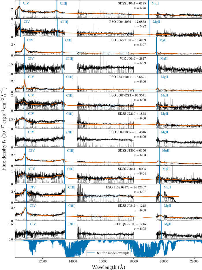
Figures 2 show the NIR spectra of all quasars in the X-SHOOTER/ALMA sample. We overplot our model fits (see Section 3) in solid orange lines and highlight the positions of the broad C iv, C iii], and Mg ii emission lines based on the quasar systemic redshift. The spectra are sorted in redshift beginning with the lowest-redshift spectrum. Wavelength ranges affected by strong telluric absorption, as seen in the telluric model example in each figure, have been removed from the spectra for display purposes. Detailed descriptions of the fits for individual quasars are provided in Appendix B.
Download figure:
Standard image High-resolution image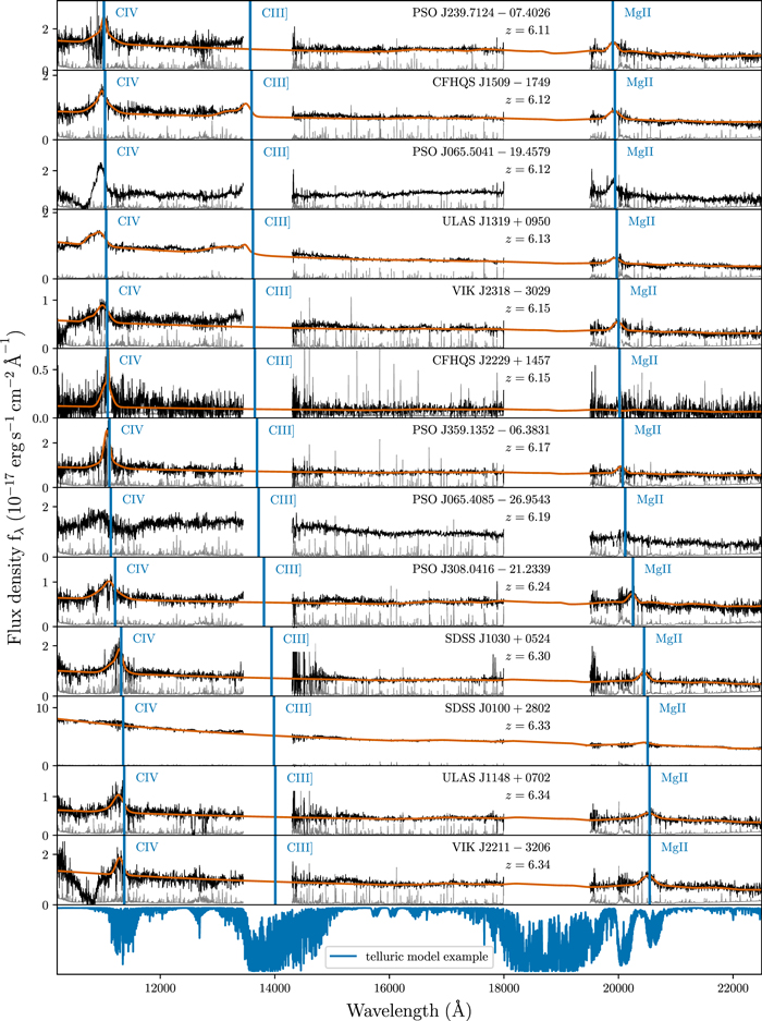
Download figure:
Standard image High-resolution image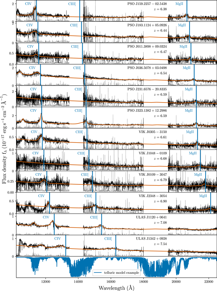
Figure 2. We display the NIR X-SHOOTER spectra of all 38 quasars in our sample. The spectra have been binned by 4 pixels, and we show the flux uncertainty in gray. Model fits are overplotted in orange for all cases where fitting the continuum with a power-law model was possible. We also highlight the positions of the broad C iv, C III], and Mg ii lines according to the systemic redshift. We have removed wavelength ranges of strong telluric absorption as highlighted by the telluric model example in the bottom panel.
Download figure:
Standard image High-resolution imageFor five quasar spectra we were not able to fit the continuum with our power-law and Balmer continuum model across the full wavelength range. These objects are PSO J009.7355–10.4316, VIK J0046–2837, PSO J065.4085–26.9543, PSO J065.5041–19.4579, and CFHQS J2100–1715 (see classification "D" in Table 2 of Appendix A). In these cases the quasar continuum flux declines blueward of the C iii] (≲1900 Å) complex. This behavior could be attributed to extinction by the quasar host galaxy or by obscuring material just outside the BLR, e.g., associated with broad absorption lines (BALs). We provide the properties of the broad C iv and Mg ii lines and the fluxes and luminosities at 1450 and 3000 Å for these five quasars by fitting the regions around the C iv line and the Mg ii line separately. Due to their intrinsic attenuation, the observed continuum luminosities should be regarded as lower limits for these quasars. Throughout this work we clearly state when these quasars are included in the analysis, and we specifically highlight them in figures with open, instead of filled, orange circles. After fully excluding instrumental effects, an in-depth study of these five sources, including a model for their extinction, is needed to further understand their nature. This is beyond the scope of this paper.
Three quasars in our sample were previously classified as BAL quasars: VIK J2348–3054 (De Rosa et al. 2014), SDSS J1044–0125 (Shen et al. 2019b), and PSO J239.7124–07.4026 (Eilers et al. 2020). We visually classify PSO J065.5041–19.4579 and VIK J2211–3206 as BAL quasars by their strong absorption blueward of C iv. An additional quasar, VIK J2318–3029, shows an absorption feature at the very blue edge of the spectrum, which potentially indicates a BAL. We will revisit its classification once the optical X-SHOOTER spectrum has been analyzed. While our sample is not a complete account of high-redshift quasars in this redshift and luminosity range, the BAL fraction of 5/38 ≈ 13% is roughly consistent with lower-redshift studies (e.g., Trump et al. 2006; Maddox et al. 2008).
Additionally, three quasars in our sample show features associated with proximate damped Lyα absorbers (pDLAs): SDSS J2310+1855 (D'Odorico et al. 2018), PSO J183.1124+05.0926 (Bañados et al. 2019b), and PSO J056.7168–16.4769 (Davies 2020; Eilers et al. 2020).
3. Modeling of the NIR Spectra
Before we start the model fitting, we pre-process the spectra. The majority of the X-SHOOTER NIR spectra have a relatively low signal-to-noise ratio (S/N) in the J band (median S/N = 6.2, 12500–13450 Å). Therefore, we bin the spectra by a factor of 4 in wavelength, increasing the median J-band S/N to 11.8. Additionally, iterative sigma clipping (>3σ) masks out the residuals of strong sky lines or intrinsic narrow absorption lines to allow for better fit results.
We then fit the NIR spectra using a custom fitting code, which is based on the LMFIT Python package (Newville et al. 2014). The code enables the user to interactively adjust the fit regions and allowed parameter ranges. A few spectral regions have to be excluded from the fit. We begin by masking out the reddest order of the X-SHOOTER NIR arm (λobs = 22500–25000 Å), which is strongly affected by high background noise from scattered light. In addition, we mask out regions with generally low S/N, which includes wavelength windows with strong telluric absorption and the blue edge of the NIR spectrum. These masked regions are λobs = 13450–14300 Å, λobs = 18000–19400 Å, and λobs ≤ 10250 Å. A figure set showing the best-fit models for each quasar, including the regions considered in the continuum and emission-line fits, accompanies this article online. An example of our best-fit model to SDSS J1306+0356 is shown in Figure 3.
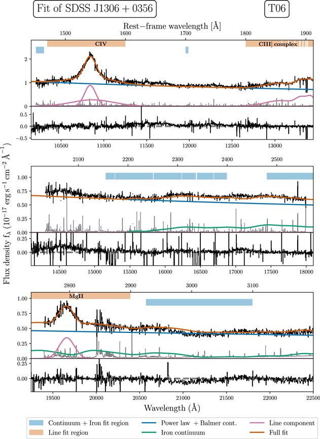
Figure 3.
Best fit to the NIR spectrum of the quasar J1306+0356 at z = 6.033. The spectrum, binned by 4 pixels, is depicted in black, with flux errors in gray. The combined fit of the continuum and the emission lines is shown as the dark-orange line. The combined power-law and Balmer continuum model is highlighted in blue, while we show the iron pseudocontinuum in green. Models for the individual emission lines are shown in purple. Light-blue and light-orange bars at the top of each panel show the regions that constrain the fit for the continuum and emission-line models, respectively. As our study focuses on the C iv and Mg ii emission lines, we have not included some other emission features seen in this spectrum. For example, the emission lines between C iv and C iii] (e.g., He ii at 1640 Å or O iii] at 1663 Å; rest frame) or the broad Fe iii features at 2000–2100 Å and 2430 Å (rest frame) are not included in the fit. We further note the iron template used in this fit in the upper right corner (T06). Best-fit figures for all quasars are available as a figure set (75 images) accompanying this paper in the online journal. (The complete figure set (75 images) is available.)
Download figure:
Standard image High-resolution imageThe spectral modeling is a two-stage process. In a first step we model the continuum components and the broad Si iv, C iv, C iii], and Mg ii emission lines. The best-fit model is saved. In the second step we estimate the uncertainties on the fit parameters. We resample each spectrum 1000 times and then draw new flux values on a pixel-by-pixel basis from a Gaussian distribution, where we assumed the original flux value to be the mean and the flux errors as its standard deviation. Each resampled spectrum is then automatically fit using our interactively determined best fit as the initial guess.
In this section we describe the assumptions and method of the fitting process. In Section 4 we briefly discuss how we measure the spectral properties and derive related quantities published along with this paper from the fits. Additional details on the spectral modeling of individual quasars are given in Appendix B.
3.1. Continuum Model
The rest-frame UV/optical spectrum of quasars is dominated by radiation from the accretion disk, which is well modeled as a single power-law component. Additionally blended high-order Balmer lines and bound-free Balmer continuum emission give rise to a Balmer pseudocontinuum, which is a nonnegligible component in the wavelength range of our NIR spectra. Transitions of single- and double-ionized iron atoms (Fe ii and Fe iii) produce an additional iron pseudocontinuum, which is especially strong around the broad Mg ii emission line. Our model of the quasar continuum includes all three components as discussed below. We do not include emission from the stellar component of the quasar host, as this can be regarded as negligible in comparison to the central engine. In general, intrinsic absorption by the quasar host can attenuate the UV/optical spectrum. However, at this point we do not consider dust attenuation in our model.
The full continuum model is fit to regions that are chosen to be free of narrow and broad quasar emission lines. Discussions of these line-free regions are provided in many references in the literature (e.g., Vestergaard & Peterson 2006; Decarli et al. 2010; Shen et al. 2011; Mazzucchelli et al. 2017; Shen et al. 2019a). As our continuum model includes contributions from the Balmer and iron pseudocontinua, we generally fit our continuum model to the following wavelength windows: λrest = 1445–1465 Å, 1700–1705 Å, 2155–2400 Å, 2480–2675 Å, and 2900–3090 Å. These continuum windows are interactively adjusted on a case-by-case basis to exclude regions with strong sky residuals, unusually large flux errors, or broad absorption features.
3.1.1. Power-law and Balmer Continuum
We model the emission of the accretion disk as a power law normalized at 2500 Å:
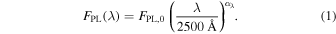
Here FPL,0 is the normalization and αλ is the slope of the power law.
The X-SHOOTER NIR arm spectral coverage only allows us to reach rest-frame wavelengths of <3400 Å for our quasar sample. As our spectra do not cover the Balmer break at λBE = 3646 Å, we only model the bound-free emission of the Balmer pseudocontinuum. For this we follow the description of Dietrich et al. (2003), who assumed that the Balmer emission arises from gas clouds of uniform electron temperature that are partially optically thick:
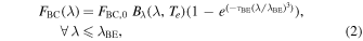
where Bλ(Te) is the Planck function at the electron temperature of Te, τBE is the optical depth at the Balmer edge, and FBC,0 is the normalized flux density at the Balmer break (Grandi 1982). Dietrich et al. (2003) discuss that the strength of the Balmer emission (FBC,0) can be estimated from the flux density slightly redward of the Balmer edge at λ = 3675 Å after subtraction of the power-law continuum. However, our wavelength range does not cover this region in the spectra. Therefore, we follow previous studies (De Rosa et al. 2011; Mazzucchelli et al. 2017; Onoue et al. 2020) and fix the Balmer continuum contribution to 30% (Dietrich et al. 2003; Kurk et al. 2007; De Rosa et al. 2011; Shin et al. 2019; Onoue et al. 2020) of the power-law flux at the Balmer edge by requiring

This choice does not affect the final results as discussed in Onoue et al. (2020). We further fix the electron temperature and the optical depth to values of Te = 15,000 K and τBE = 1, common values in the literature (Dietrich et al. 2003; Kurk et al. 2007; De Rosa et al. 2011; Mazzucchelli et al. 2017; Shin et al. 2019; Onoue et al. 2020).
3.1.2. Iron Pseudocontinuum
Careful analysis of the quasar continuum and the properties of the broad emission lines is complicated by the presence of atomic and ionic iron in the BLR. The large number of electron levels in iron atoms leads to a multitude of emission-line transitions, especially from Fe ii, throughout the entire spectral region probed in this study. Due to the large velocities of the BLR clouds, the weak iron emission lines are broadened and blend into a pseudocontinuum, hindering our analysis of the C iv, C iii], and Mg ii emission lines. Empirical and semiempirical iron templates, derived from the narrow-line Seyfert 1 galaxy I Zwicky 1 (Boroson & Green 1992; Vestergaard & Wilkes 2001; Tsuzuki et al. 2006), allow us to easily incorporate iron emission into spectral fitting routines. For our analysis we use both the Tsuzuki et al. (2006, hereafter T06) template and the Vestergaard & Wilkes (2001, hereafter VW01) template.
T06 and VW01 discuss that subdividing the iron template into segments may be necessary as the individual emission strengths of the iron multiplets vary across the spectrum. VW01 discuss that their undivided iron template overpredicts the iron emission in the λrest = 1400–1530 Å region. Based on this insight, we divided the iron template into two segments, one covering the C iv (VW01) line and one covering the Mg ii (T06) line, and performed test fits on a few spectra. We discovered that we were not able to constrain the weak iron emission around the C iv at rest-frame wavelengths of λrest = 1200–2200 Å. Therefore, we only incorporate an iron template in our continuum model to separate the Mg ii line from the underlying iron pseudocontinuum at rest-frame wavelengths of λrest = 2200–3500 Å.
In contrast to the purely empirical VW01 template, in which iron emission beneath the broad Mg ii line is not included, T06 were able to model this iron contribution using a spectral synthesis code and add it to their template. The difficulties in fitting the Fe contribution in quasar spectra are discussed in many studies throughout the literature (e.g., Boroson & Meyers 1992; Vestergaard & Wilkes 2001; Tsuzuki et al. 2006; Woo et al. 2018; Shin et al. 2019; Onoue et al. 2020). A detailed analysis on covariance between the iron contribution and the power-law fit is given in De Rosa et al. (2011). We will expand on this discussion based on the quantitative results of our sample in Section 5.
The original iron emission in the I Zwicky 1 templates has an intrinsic width of FWHM ≈ 900 kms−1. Therefore, to accurately model the iron emission in our spectra, we broaden the iron templates by convolving them with a Gaussian kernel to match the FWHM of the broad Mg ii line:
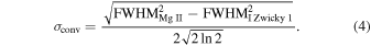
While the broadening of the iron emission is necessary to study quasars (e.g., Boroson & Green 1992), our approach is most similar to T06 and Shin et al. (2019), who also use the FWHM of the Mg ii line as a proxy for the velocity dispersion of the BLR. Shin et al. (2019) compare how a similar assumption influences the measurement of the Fe ii/Mg ii flux ratio. The authors constrain the Fe ii pseudocontinuum velocity dispersion within 10% of the Mg ii FWHM and find Fe ii/Mg ii flux ratios consistent with each other within 7% compared to leaving the iron FWHM as a free parameter. Hence, we are confident that this assumption only has a minor influence on our best-fit measurements.
In addition to the FWHM, we also set the iron template redshift to the redshift of the broad Mg ii line. As the iron template and the Mg ii fits are interdependent, we iteratively fit the full continuum model and the Mg ii line. In each step we update the iron template parameters after the Mg ii line fit until the FWHM and the redshift of the Mg ii line converge.
3.2. Emission-line Models
Our analysis focuses on the broad emission lines Si iv, C iv, C iii], and Mg ii. All four lines are doublets. However, their broad nature, along with the modest S/N of our spectra, does not allow us to resolve them. Therefore, these lines are modeled as single broad lines at rest-frame wavelengths of 1396.76 Å for Si iv, 1549.06 Å for C iv, 1908.73 Å for C iii], and 2798.75 Å for Mg ii (see Vanden Berk et al. 2001). We provide an overview of the lines modeled in each quasar spectrum in Table 1.
3.2.1. Mg ii Emission Line
The majority of the analyzed X-SHOOTER NIR spectra detect the Mg ii line with a low S/N (median S/N = 8.6) even in the binned spectra. Hence, we decided to model the Mg ii line with a single Gaussian profile only. The line is generally fit over rest-frame wavelengths of λrest = 2700–2900 Å, similar to Shen et al. (2019a). We adjust this wavelength range to mask out regions with absorption lines, bad sky subtraction, or noisy telluric correction. We vary the model parameters to find the best fit of the redshift, the FWHM, and the amplitude of the Gaussian profile, assuming a rest-frame central wavelength of 2798.75 Å (Vanden Berk et al. 2001).
3.2.2. C iv Emission Line
In comparison to the Mg ii emission line, the C iv line is known to often exhibit asymmetric line profiles associated with an outflowing wind component (e.g., Richards et al. 2011). We always start by using two Gaussian profiles to model the C iv line, which allows us to account for this asymmetry. However, not all lines are asymmetric, and spectra with very low S/Ns or strong absorption lines often cannot constrain a two-component model. Therefore, we fit the C iv line with a single Gaussian component (1G) in nearly half of our sample (see Table 1). We fit the C iv line in a rest-frame wavelength window of λrest = 1470–1600 Å. Quasars at high redshift are known to exhibit highly blueshifted C iv compared to their other emission lines (e.g., Meyer et al. 2019). Therefore, we have slightly extended the fitting range blueward compared to Shen et al. (2011, 2019a). Equivalent to the Mg ii line fit, the central wavelength (redshift), the FWHM, and the amplitude of each Gaussian component are optimized independent of each other to find the best fit. The line properties are then determined from the combined components of the line fit.
3.2.3. C iii] Emission Line
The C iii] emission line falls into the telluric absorption window between the J and H bands in the redshift range of z ≈ 6–6.5. Thus, we were able to determine properties related to the line only for a subset of our X-SHOOTER spectra. In addition, the proximity of the Al iii λ1857.40 and Si iii] λ1892.02 emission lines to the C iii] λ1908.73 line complicates the modeling. This is especially true in quasar spectra, where these lines are usually blended owing to the large velocity dispersion of the broad emission lines. Each of the three lines is modeled with a single Gaussian profile. While we allow for independent variations of the amplitude and FWHM of the three Gaussian profiles, they are fit to the same redshift using the rest-frame line centers provided above. The region over which the lines are fit is always adjusted manually owing to the proximity to wavelength regions with strong telluric absorption.
The combination of the three lines provides a reasonable fit in most cases. However, the individual line contributions of the strongly degenerate Si iii] and C iii] lines cannot be separated with certainty. Therefore, we only extract peak redshift measurement from the C iii] complex (sum of all three line models) fits and disregard other properties. In order to properly fit the C iii] complex in a few quasar spectra, it was necessary to set the contributions of the Al iii and Si iii] lines to zero. These details are given in Appendix B.
3.2.4. Si iv Emission Line
In quasars at z ≳ 6.4 the broad Si iv λ1396.76 emission line redshifts into the wavelength range of the X-SHOOTER NIR spectra. The broad nature of the Si iv line results in a line blend with the close-by semiforbidden O IV] λ1402.06 transition. Because we cannot disentangle the two lines, we decided to model their blend, Si iv+O IV] λ1399.8,14 using one Gaussian component.
The throughput and thus the S/N decline toward the blue edge of the X-SHOOTER NIR spectra. In addition, strong BALs blueward of the C iv line complicate the continuum modeling in a few cases. As a result, we were only able to successfully fit the Si iv line in the spectra of four quasars: PSO J036.5078+03.0498, ULAS J1120+0641, ULAS J1342+0928, and PSO J323.1382+12.2986 (see Tables 7 and 8).
3.3. Overview of the Fitting Process
We briefly summarize the steps of the fitting process:
- 1.We bin every 4 pixels of the fully reduced X-SHOOTER NIR spectra and mask out strong sky-line residuals with iterative sigma clipping.
- 2.We mask out all regions of strong telluric absorption.
- 3.We add the power-law and Balmer continuum model to the fit. The power-law and Balmer continuum redshift is set to the [C ii] or Lyα halo redshift. In the few cases where no accurate systemic redshift is available, we set the continuum redshift to the best systemic redshift in the literature and reevaluate this redshift based on our fit to the Mg ii emission line.
- 4.We further add the iron template and set the initial redshift to the systemic redshift from the literature and provide an initial guess for the FWHM.
- 5.We fit the full continuum model (power law + Balmer continuum + iron template).
- 6.Then, we add the Mg ii emission-line model and fit it to determine its FWHM and redshift.
- 7.We iteratively refit the full continuum model and the Mg ii emission line (steps 5 and 6), applying the Mg ii FWHM and redshift to the iron template until the Mg ii line fit converges. This takes about four to six iterations.
- 8.In the next step we include the C iv model and if possible the C iii] and Si iv models in the line fit.
- 9.The best model fit and its parameters are then saved. A separate routine resamples the science spectrum 1000 times using its noise properties, bins the spectrum by every 4 pixels, and then refits it using the saved model with the best-fit parameters as the first guess.
4. Analysis of the Fits
For each best fit in the refitting process we not only determine the values of all fit parameters but also calculate all derived quantities. This extends, for example, to BH mass estimates and Fe ii/Mg ii flux ratios. We resample and refit each spectrum 1000 times, resulting in distributions for each fit parameter and derived quantity. The results presented in this paper quote the median of this distribution, and the associated uncertainties are the 15.9 and 84.1 percentile values. A machine-readable online table summarizes all fit results. Table 9 in Appendix C presents the columns of this table for an overview.
4.1. Continuum
We derive the flux densities and luminosities at wavelengths 1350 Å, 1400 Å, 1450 Å, 2100 Å, 2500 Å, and 3000 Å from the power-law continuum model, including the Balmer continuum contribution. In the case of the five spectra, for which we could not model the continuum with a power law, we perform local fits to the continuum around the regions of the C iv and Mg ii lines to determine the continuum fluxes at 1400 Å, 1450 Å, and 3000 Å.
Based on the flux density at 1450 Å, we also calculate the apparent and absolute magnitudes, m1450 and M1450. In some cases the flux densities at 1350 Å (z ≲ 6.59), 1400 Å (z ≲ 6.32), and 1450 Å (z ≲ 6.08) were measured by extrapolating the fit blueward, outside of the spectral range of the X-SHOOTER NIR arm.
For our main analysis we estimate the bolometric luminosity following Shen et al. (2011):

We further determine the integrated flux and the luminosity of the Fe ii pseudocontinuum in the wavelength range of 2200–3090 Å, to construct Fe ii/Mg ii flux ratios as discussed in Section 6.1.
4.1.1. Emission Lines
For the Si iv, C iv, and Mg ii lines we calculate the peak wavelength from the maximum flux value of the full-line model (all components). As most of the C iv line models consist of two Gaussian components, these are added before the peak of the line model is determined. The line redshift follows from the peak wavelength of the line model and the corresponding rest-frame wavelength of the line. Velocity shifts of the lines are derived from their line redshift in comparison to the systemic [C ii] redshift using linetools (Prochaska et al. 2016) including relativistic corrections. We also compute the FWHM, equivalent width (EW), integrated flux, and integrated luminosity of all lines using the full-line model, hence taking into account all line components. In the resampling process catastrophic fits of multicomponent lines can occur, where the component peaks are too separated to allow a successful determination of the FWHM. These cases are rare and not taken into account for the final FWHM measurements. All FWHM measurements are corrected for instrumental line broadening introduced by the resolution of the X-SHOOTER spectrograph.
We already discussed the complications in inferring line properties of the strongly blended lines in the C iii] complex. Therefore, we only extract the C iii] complex redshift from the peak flux of the full C iii] complex (sum of all three lines).
4.1.2. Black Hole Mass Estimates
We provide estimates of the BH masses along with this paper. While these results will be discussed in detail in E. P. Farina et al. (2020, in preparation), we include a discussion on how they were estimated in Appendix D for completeness.
5. Systematic Effects on Mg ii Measurements Introduced by the Choice of the Iron Template
The broad Mg ii line lies in a spectral region where a plethora of Fe ii emission lines form a strong pseudocontinuum in many quasar spectra. Hence, it is important to take the contribution of Fe ii emission into account when modeling the Mg ii line to derive unbiased properties. This can be achieved by either using scaled and broadened (semi)empirical iron templates or calculating full model spectra using a spectral synthesis code. In this work we have chosen the former approach, adopting the iron templates of VW01 and T06. The empirical iron template of VW01 has been widely used in the literature (e.g., De Rosa et al. 2011; Mazzucchelli et al. 2017). It is derived from the spectrum of the narrow-line Seyfert 1 galaxy I Zwicky 1 and covers the entire UV rest-frame range of the AGN. However, at the time the authors were not able to estimate the strength of the Fe ii pseudocontinuum beneath the Mg ii line. Therefore, they made the conscious decision to underestimate the iron continuum contribution and set it to zero beneath the Mg ii line (see their Section 3.4.1 in VW01). A few years later T06 used the spectral synthesis code CLOUDY (Ferland et al. 1998) to model the iron contribution beneath the Mg ii line and created a semiempirical iron template based on these synthetic iron spectra and the observed spectrum of I Zwicky 1. Differences in the iron flux contribution of various iron templates in the literature account for one of the major uncertainties in modeling the Mg ii line, as well as the iron flux itself (e.g., Dietrich et al. 2003; Kurk et al. 2007; Woo et al. 2018; Shin et al. 2019).
In fitting each of our spectra with both the VW01 iron template and the T06 iron template, we assess these differences quantitatively to understand possible biases in our measurements. In Figure 4 we show both fits around the Mg ii line for ULAS J1148+0702 at z = 6.339. Solid lines refer to the fit with the T06 template, and dashed lines refer to the model fit using the VW01 iron template. This example highlights how the full fit of both models (orange solid and gray dashed lines) is nearly identical. On the other hand, the line fit component (purple lines) and the iron template component (green lines) are significantly different. All derived fit parameters of the Mg ii line (FWHM, integrated line flux, and central wavelength), as well as the integrated flux of the iron component, are affected.
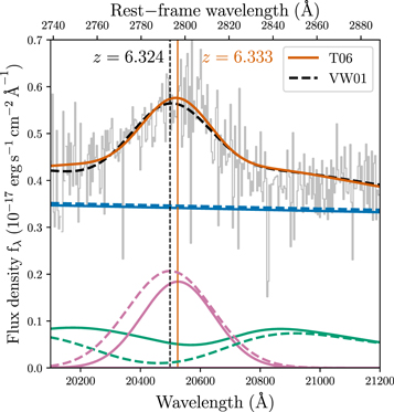
Figure 4. Comparison of the model fits to quasar ULAS J1148+0702 using the two different iron templates of T06 and VW01. Solid lines denote the T06 model fit, while dashed lines show the VW01 model fit. The model fit components are colored as in Figure 3. While the full fit (black/orange) lines are very similar, the iron template (green) and the Mg ii line components (purple) differ considerably, resulting in different best-fit parameters for the width, amplitude, and center of the line.
Download figure:
Standard image High-resolution imageIn Figure 5 we compare the model fit results for each template in a subsample of 28 quasars, which have both successful Mg ii line fits and [C ii] redshifts. These 28 quasars are marked in Table 5 for reproducibility. Orange colors in Figure 5 refer to the T06 iron template and blue colors to the VW01 template. Dashed–dotted lines in the figure depict the median values of each property, which we also compare in Table 3.
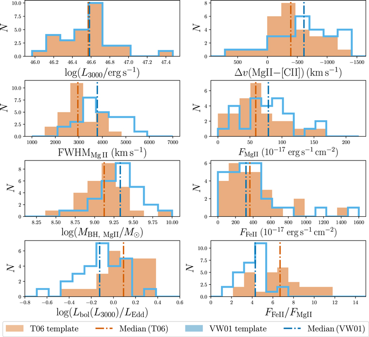
Figure 5. Histograms of the main Mg ii and Fe ii properties highlighting the differences due to the use of either the T06 or the VW01 iron template in the model fit. The FWHM of Mg ii and its integrated flux, FMgii, are most affected by the choice of the iron template. By extension, all dependent properties are affected as well. A total of 27 quasars with a successful fit of the Mg ii line and secure [C ii] redshifts contribute to the histograms. The dashed–dotted lines show the median of the distributions. Results based on the T06 template are colored orange, while results from the VW01 template are colored blue. The panels, from top left to bottom right, show the luminosity at 3000 Å (L3000), the blueshift of Mg ii with respect to the [C ii] line, the FWHM of Mg ii, the Mg ii integrated flux, the derived BH mass using the relation of Vestergaard & Osmer (2009), the integrated flux of the iron template between 2200 and 3090 Å, the Eddington luminosity ratio based on the shown BH mass, and the flux ratio of the iron and Mg ii fluxes.
Download figure:
Standard image High-resolution imageTable 3. Comparison of the Best-fit Properties Based on Model Fits with Two Different Iron Templates
| Property | Median | Median |
|---|---|---|
| T06 Template | VW01 Template | |
|
46.57 | 46.58 |
| Δv(Mgii − [Cii])/(km s−1) | −390.61 | −612.17 |
| FWHMMg II/(km s−1) | 2955.52 | 3785.64 |
| log (MBH,Mgii/M⊙) | 9.12 | 9.33 |
| Lbol(L3000)/LEdd | 1.23 | 0.75 |
| FMgii/(10−17 erg s−1 cm−2 Å−1) | 59.10 | 78.84 |
| FFeII/(10−17 erg s−1 cm−2 Å−1) | 363.25 | 319.06 |
| FFeII/FMgii | 6.70 | 4.30 |
Note. We contrast the median values for a subsample of 28 quasars with secure [Cii] redshifts.
Download table as: ASCIITypeset image
As suggested by the example fit in Figure 4, measurements of the joint power-law and Balmer continuum model (solid and dashed blue lines) remain largely unaffected by the choice of the iron template. The median values of L3000 measured from the two different templates are nearly identical (see top left panel of Figure 5 and Table 3).
Figure 5 highlights how all other properties show systematic differences. We illustrate the influence of the templates on the Mg ii redshift by analyzing the Mg ii velocity shift with respect to the systemic redshift of the [C ii] line, Δv(Mgii − [Cii]). The distributions for the velocity shifts appear similar (Figure 5, top right) at first, but the difference in median velocity shift is nonnegligible between the templates, ∼200 km s−1 (see Table 3), considering that the absolute values for the median velocity shifts are around −400 to −600 km s−1. In consequence, measurements of the C iv–Mg ii velocity shift will be affected. However, the often large C iv blueshifts of ∼1000 km s−1 will render this bias less relevant. The reason for these differences is the asymmetry in the iron contribution underlying the Mg ii line in the T06 template, whereas the missing iron emission in the VW01 template is largely symmetric around the line. The comparison of the iron templates (green lines) in Figure 4 highlights this difference. Hence, the choice of the iron template has an effect on the best-fit redshift of the Mg ii line.
As previously discussed in Woo et al. (2018), the measured FWHM of the Mg ii is also affected by the iron template used. The model fits of the Mg ii (purple lines) in Figure 4 emphasize this. The choice of the VW01 template results in a broader line fit. The histogram of the FWHMMgii in Figure 5 (second panel in the left column) makes this systematic shift toward broader FWHMMgii evident. Compared to the T06 template, the median FWHMMgii measured with the VW01 template is broader by ∼800 km s−1 (Table 3). Consequently, the derived BH masses and Eddington luminosity ratios are shifted as can be seen in the lower two panels in the left column of Figure 5. We have derived the BH mass estimates using the relation of Vestergaard & Osmer (2009), which was established using the iron template of VW01. The scaling relation and the conversion to Eddington luminosity both use the continuum luminosity at 3000 Å, L3000, which is largely unaffected by the choice of the iron template. Therefore, the shifts in distributions and medians of the BH masses and Eddington luminosity ratios are a direct consequence of the difference in the measured FWHMMgii. The larger FWHMMgii values from the use of the VW01 template result in larger BH masses and lower Eddington luminosity ratios. It is worth noting that the use of the VW01 template compared to the T06 template moves the median of the Eddington luminosity ratio from a super-Eddington value to a sub-Eddington value for this subset of the X-SHOOTER/ALMA sample.
5.1. The Effect on the Fe ii/Mg ii Ratio
The choice of the iron template has its most profound effect on the Fe ii/Mg ii flux ratio, a proxy for the Fe/Mg abundance and therefore for the iron enrichment of BLR gas in high-redshift quasars (see, e.g., Dietrich et al. 2003). Figure 4 shows that the model fits using the two templates result in a nearly equivalent fit of the Mg ii region. The difference between the fits is the flux contribution of the line model and the Fe ii pseudocontinuum to the total fit. Using the VW01 template results in significantly larger Mg ii and smaller Fe ii fluxes as can be seen in Figure 5 (middle panels in the right column) or in panel (a) of Figure 6. The trends have also been discussed in the literature (Dietrich et al. 2003; Shin et al. 2019). As a consequence, the resulting Fe ii/Mg ii flux ratios are much smaller compared with the T06 template (Figure 5, bottom right panel). However, the effect does not simply shift the FMgii toward larger values when changing from the T06 template to the VW01 template. Panel (a) of Figure 6 clearly shows that quasars with stronger Fe ii emission are affected more significantly. As a result, the distribution of FMgii in Figure 5 (second panel in the right column) also changes its shape and the median value increases strongly from ∼59 × 10−17 ergs−1 cm−2 to ∼79 × 10−17 erg s−1 cm−2. Most model fits to the spectra will result in an equally good fit for both templates. Therefore, a larger FMgii has to result in a reduced iron continuum flux, FFeII. This is indeed seen in both panel (a) of Figure 6 and Figure 5 (third panel in the right column). The effect on the FFeII does not appear significant at first. Integrated over rest-frame wavelengths of 2200 to 3090 Å, the iron median flux is much larger than that of the Mg ii line. However, both effects conspire to result in a severe systematic effect on the Fe ii/Mg ii flux ratio, FFeII/FMgii. Using the VW01 template, FFeII/FMgii reaches a median value of 4.30, which increases by a factor of ∼1.5 to FFeII/FMgii = 6.70 when the T06 template is assumed. Panel (b) of Figure 6 shows how FFeII/FMgii changes between the two different templates. In an attempt to characterize the relationship between the Fe ii/Mg ii flux ratios resulting from the two different templates, we have fit the data in Figure 6(b) with orthogonal distance regression15 modeled by a second-order polynomial model without the constant term:
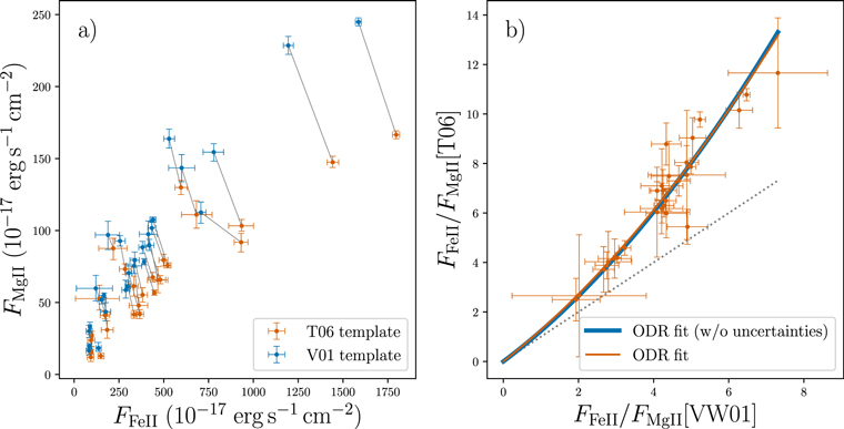
Figure 6. Influence of the iron template on the FFeII/FMgii ratios. (a) Mg ii flux as a function of Fe ii flux. The change from the T06 (orange) to the VW01 (blue) template introduces a diagonal shift (gray line) of the data points toward lower Fe ii and higher Mg ii flux. (b) Comparison between the flux ratios calculated with both templates. We show our best fit using orthogonal distance regression as the orange solid line. The solid blue line shows the same fit excluding the measurement errors. The FFeII/FMgII ratio data based on the T06 template clearly lie above the 1:1 relation (gray dotted line).
Download figure:
Standard image High-resolution imageThe model assumes that both flux ratios are equal at the origin. The blue lines in panel (b) of Figure 6 show our fit results with (orange line; a = 0.083 ± 0.021, b = 1.198 ± 0.111) and without (blue line; a = 0.094 ± 0.032, b = 1.136 ± 0.152) including the uncertainties on the flux ratios. The nonzero second-order component in both model fits shows that the scaling between the flux ratio values from one template to the other is distinctly nonlinear. The majority of quasars in our sample have flux ratios between 4 and 5 based on the VW01 template, resulting in scale factors of 1.53−1.61, in good agreement with the median scaling of the flux ratios determined earlier (∼1.56). These model fits allow us to compare literature values of FFeII/FMgii based on the VW01 template to our new values derived using the T06 template in Section 6.1.
5.2. On the Future Use of Different Iron Templates
Because the T06 iron template includes the Fe ii continuum contribution beneath the Mg ii line, we adopt it for our line analysis. Future studies focused on the Mg ii line properties (FWHM, redshift, line flux), the Fe ii continuum, and the FFeII/FMgII should consider using the T06 iron template or any equivalent iron template, which includes the Fe ii continuum beneath the Mg ii line.
However, one has to be very careful when it comes to the derivation of BH mass estimates and, subsequently, Eddington luminosity ratios based on the Mg ii line. The majority of single-epoch virial estimators (e.g., Vestergaard & Osmer 2009; McLure & Dunlop 2004, both applied in this work) use the VW01 iron template, when constructing the scaling relations of Mg ii from the Hβ line. Therefore, estimates of BH masses derived from the Mg ii line need to be based on the same iron template, with which the scaling relation was originally established. Otherwise, one will risk systematic biases in the BH masses and Eddington luminosity ratios as shown in Figure 5. For example, the use of the T06 template in combination with the Vestergaard & Osmer (2009) scaling relation erroneously gave the impression that our sample has a large fraction of quasars showing super-Eddington accretion. At last, we should remind ourselves that both the T06 and VW01 templates are based on a single, low-redshift, low-luminosity Seyfert galaxy and thus may have limited applicability for the high-redshift quasar population.
6. Results
6.1. Iron Enrichment Traced by High-redshift Quasars
One possible way to trace the buildup of metals in the galaxy's ISM is by measuring the abundance ratio of iron to α-process elements. While α-process elements are predominantly produced in core-collapse Type II supernovae (SNe II), which have massive star progenitors, Fe is released into the ISM mainly from Type Ia supernovae, which follow the evolution of intermediate, binary stars. The difference in evolutionary lifetimes leads to a delay of the enrichment of iron compared to α-process elements, which has been estimated to be around 1 Gyr (e.g., Matteucci & Greggio 1986). However, it has also been shown that this delay can be as short as ∼0.2–0.6 Gyr (Matteucci 1994; Friaca & Terlevich 1998; Matteucci & Recchi 2001) in the case of elliptical galaxies.
In high-redshift quasars we can measure the Fe ii/Mg ii flux ratio, which has been widely used in the literature as a proxy for the Fe/Mg abundance ratio to estimate iron enrichment in the quasar's BLR (e.g., Dietrich et al. 2002; Iwamuro et al. 2002; Barth et al. 2003; Dietrich et al. 2003; Freudling et al. 2003; Maiolino et al. 2003; Iwamuro et al. 2004; Kurk et al. 2007; De Rosa et al. 2011, 2014; Mazzucchelli et al. 2017; Sameshima et al. 2017; Shin et al. 2019, and references therein).
We construct the Fe ii/Mg ii flux ratio from the total integrated flux of the Mg ii line model and the flux of the iron template integrated over the wavelength range of 2200–3090 Å. The wavelength range has been chosen to be comparable to the literature on this topic, as the choice impacts the Fe ii/Mg ii flux ratio measurement. We provide the measured Fe ii and Mg ii fluxes and the Fe ii/Mg ii flux ratio measured with both the VW01 and T06 templates in Table 4. We were able to successfully fit the Mg ii line and the iron pseudocontinuum in 32 quasars from our sample and calculate FFeII/FMgii for these objects.
Table 4. Fe ii/Mg ii Flux Ratios
| Quasar Name | FFeIIa (T06) | FMgiib (T06) | FFeII/FMgiic | FFeIIa (VW01) | FMgiib (VW01) | FFeII/FMgiic |
|---|---|---|---|---|---|---|
| (10−17 erg s−1cm2) | (T06) | (10−17 erg s−1cm2) | (VW01) | |||
| PSO J007.0273+04.9571 |

|

|

|

|

|

|
| PSO J011.3898+09.0324 |

|

|

|

|

|

|
| VIK J0046–2837 |

|

|

|

|

|

|
| SDSS J0100+2802 |

|

|

|

|

|

|
| VIK J0109–3047 |

|

|

|

|

|

|
| PSO J036.5078+03.0498 |

|

|

|

|

|

|
| VIK J0305–3150 |

|

|

|

|

|

|
| PSO J056.7168–16.4769 |

|

|

|

|

|

|
| PSO J065.4085–26.9543 |

|

|

|

|

|

|
| PSO J065.5041–19.4579 |

|

|

|

|

|

|
| SDSS J0842+1218 |

|

|

|

|

|

|
| SDSS J1030+0524 |

|

|

|

|

|

|
| PSO J158.69378–14.42107 |

|

|

|

|

|

|
| PSO J159.2257–02.5438 |

|

|

|

|

|

|
| VIK J1048–0109 |

|

|

|

|

|

|
| ULAS J1148+0702 |

|

|

|

|

|

|
| PSO J183.1124+05.0926 |

|

|

|

|

|

|
| SDSS J1306+0356 |

|

|

|

|

|

|
| ULAS J1319+0950 |

|

|

|

|

|

|
| CFHQS J1509–1749 |

|

|

|

|

|

|
| PSO J231.6576–20.8335 |

|

|

|

|

|

|
| PSO J239.7124–07.4026 |

|

|

|

|

|

|
| PSO J308.0416–21.2339 |

|

|

|

|

|

|
| SDSS J2054–0005 |

|

|

|

|

|

|
| CFHQS J2100–1715 |

|

|

|

|

|

|
| PSO J323.1382+12.2986 |

|

|

|

|

|

|
| VIK J2211–3206 |

|

|

|

|

|

|
| PSO J340.2041–18.6621 |

|

|

|

|

|

|
| SDSS J2310+1855 |

|

|

|

|

|

|
| VIK J2318–3029 |

|

|

|

|

|

|
| VIK J2348–3054 |

|

|

|

|

|

|
| PSO J359.1352–06.3831 |

|

|

|

|

|

|
Notes.
aThe Fe ii flux is calculated from the iron pseudocontinuum integrated over the wavelength range of 2200–3090 Å. bThe Mg ii flux has been integrated over the complete Mg ii line model. cThe Fe ii/Mg ii flux ratio is calculated during the resampling process. Therefore, the median value of the flux ratio might deviate from the ratios of the median flux values.Download table as: ASCIITypeset image
We now turn to comparing our results with other measurements in the literature to cover a wide redshift range 0 ≤ z ≤ 7.5 as shown in Figure 7. A comparison between Fe ii/Mg ii flux ratios across many studies is often complicated by differences in their measurements (see, e.g., Kurk et al. 2007; De Rosa et al. 2011; Shin et al. 2019; Onoue et al. 2020, for discussions). Fitting methodology (algorithms, assumed iron template, iron integration wavelength range) varies from study to study, resulting in differences in the measured Fe ii/Mg ii flux ratio (Section 5). A good discussion on the impact of the assumed Balmer continuum strength is given in Onoue et al. (2020). The authors find that reducing the strength of the Balmer continuum model only slightly lowers the measured Fe ii/Mg ii flux ratio. We first select studies that provide an Fe ii/Mg ii flux ratio measurement with the T06 iron template and the same Fe ii flux integration range used in our work (Shin et al. 2019; Onoue et al. 2020). Then, we add measurements, for which the VW01 template was used in the same integration range (Dietrich et al. 2003; Maiolino et al. 2003; Mazzucchelli et al. 2017). To compare these data with our Fe ii/Mg ii flux ratios, we scale the mean literature values using Equation (6). We further use the results of De Rosa et al. (2011), of a sample of quasars at z ≈ 4.5–5 and z ≈ 5.8–6.5. The authors use the same rest-frame wavelength range to integrate the Fe ii flux and the VW01 template, but they add a constant flux density at 2770–2820 Å equal to 20% of the mean flux density of the template between 2930 and 2970 Å (see also Kurk et al. 2007). This modification to the VW01 template was motivated by the missing Fe flux beneath the Mg ii line. As discussed in Shin et al. (2019), this modification only slightly increases the average Fe ii/Mg ii flux ratio by ∼6%. We therefore reduce the Fe ii/Mg ii accordingly and then apply Equation (6) to the De Rosa et al. (2011) results. To populate the redshift range below z = 2, we add the median values of Iwamuro et al. (2002) to our comparison. However, this comparison is not ideal, as the authors extracted their own iron template from the Large Bright Quasar Survey composite spectrum (Francis et al. 1991) and integrated the fitted template over a rest-frame wavelength of 2150–3300 Å to calculate the Fe ii flux.
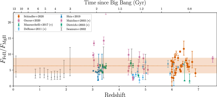
Figure 7. Fe ii/Mg ii flux ratio as a function of redshift. The z > 2 data do not show any significant evolutionary trend with redshift. Our measurements using the T06 iron template are shown as filled and open orange circles. The open circles refer to spectral fits, in which the continuum was only approximated locally around the Mg ii, including the iron contribution. We further display the median value of our sample with the dashed orange line and the 16th to 84th percentile region in light orange. Different colored data points show literature values from previous studies (Dietrich et al. 2003; Maiolino et al. 2003; De Rosa et al. 2011; Mazzucchelli et al. 2017; Shin et al. 2019; Onoue et al. 2020), which either are using the T06 template as well or are scaled appropriately (*) from the VW01 template using Equation (6). At lower redshift we display the median values from the study of Iwamuro et al. (2002), which are based on their own iron template. We discuss the comparability of the different measurements in Section 6.1 in more detail.
Download figure:
Standard image High-resolution imageFigure 7 shows our results as open and filled orange circles. The open circles refer to quasars, which could not be modeled with a continuous power-law model from C iv to Mg ii (see Section 2.3). The uncertainties on the flux ratio measurement reflect the S/N of the binned spectra. Different colored symbols show previous results from the literature (Dietrich et al. 2003; Maiolino et al. 2003; De Rosa et al. 2011; Mazzucchelli et al. 2017; Shin et al. 2019; Onoue et al. 2020, as discussed above). Gray data points are the median values from the study of Iwamuro et al. (2002).
Our results presented in context with the literature data in Figure 7 do not show any discernible evolutionary trend with redshift. Keeping in mind that the exact measurement (iron template, wavelength integration range, etc.) differs from study to study, our result echoes the findings of many previous studies (e.g., Barth et al. 2003; Dietrich et al. 2003; Freudling et al. 2003; Maiolino et al. 2003; Kurk et al. 2007; De Rosa et al. 2011, 2014; Mazzucchelli et al. 2017; Shin et al. 2019; Onoue et al. 2020). We measure a median value of  for our sample of 32 quasars. The errors denote the 16th to 84th percentile range on the median measurement. It should be noted that this value is different from the value in Table 3 (FFeII/FMgii = 6.70), as we now include four more quasars, whose systemic redshifts were determined from the Lyα halo or using the Mg ii line. Excluding the four quasars, whose continuum significantly deviates from a power law (open orange circles in Figure 7), we calculate a median value of
  . The median value is the same as before, but the 16th to 84th percentile range narrows significantly.
Our Fe ii/Mg ii flux ratios are similar to values from lower-redshift samples even if lower-luminosity quasars (Shin et al. 2019, with Lbol ≈ 46.5) are considered. The only exception are the results of Iwamuro et al. (2002) at z ≈ 1–2. In this redshift range the authors find median values up to FFeII/FMgii ∼ 5. However, their use of a different iron template might be the cause of the discrepancy in the measurements. At z = 7.54 we have included the FeII/Mgii flux ratio of ULAS 1342+0928 from Onoue et al. (2020) measured from a deep GNIRS spectrum. While this quasar is also part of our sample, the Mg ii line falls into the reddest order, which is dominated by the noise. Therefore, we were not able to constrain the Mg ii properties. The Fe ii/Mg ii flux ratio of ULAS 1342+0928 is relatively high compared to our median, but well within the 16th–84th percentile range.
6.1.1. Discussion
We have so far assumed that the Fe ii/Mg ii flux ratio in quasars is a good tracer of the Fe/Mg abundance ratio. Therefore, approaching higher and higher redshift, we would expect the Fe ii/Mg ii flux ratio to first peak and decline significantly following the predictions of Fe/α enrichment (e.g., Sameshima et al. 2017, their Figure 17). However, our results, along with the data from the literature (see Figure 7), do not show a significant evolution of FFeII/FMgii at the highest redshifts. As no decrease is evident with redshift, this would indicate, at face value, that the central part of the host galaxy is already sufficiently enriched in iron in all luminous quasars at z ∼ 7, ∼750 Myr after the big bang and even in the most distant quasar ULAS 1342+0928 (Onoue et al. 2020), another ∼70 Myr before. Given the delay time of ∼0.2–0.6 Gyr (Matteucci 1994; Friaca & Terlevich 1998; Matteucci & Recchi 2001), this would indicate that the first episode of star formation in these quasar hosts would have had to have occurred at z ≳ 9.
However, this result only holds if the physical conditions for the excitation of Fe ii and Mg ii are the same (or at least similar) in all quasars at all redshifts and if the Fe ii/Mg ii flux ratio actually traces the Fe/Mg abundance. Photoionization calculations (Verner et al. 2003; Baldwin et al. 2004) suggest that the Fe ii/Mg ii flux ratio does depend on physical parameters of the BLR, like gas density, microturbulence, and the properties of the radiation field. Photoionization models of Sameshima et al. (2017) further indicate that the Mg ii line strength is dependent on the density of the BLR gas. In their sample of ∼17,000 quasars at z = 0.72–1.63 they identify an observational anticorrelation between the Fe ii/Mg ii flux ratio and the Eddington luminosity ratio. The authors suspect the accretion rate and the gas density to be interdependent, which in turn leads to the anticorrelation with the Eddington luminosity ratio.
We evaluated the Pearson correlation coefficient and found both properties to be uncorrelated with ρ = 0.02 and p = 0.93 in our sample. Yet we should keep in mind that our quasars only sample a small range of Eddington luminosity ratios. As studies continue to identify nonabundance dependencies of the Fe ii/Mg ii flux ratio on the physical conditions of the BLR, there is no doubt that we need to be careful when interpreting it in the context of iron enrichment. However, ALMA observations of high-redshift quasar host galaxies have detected large amounts of dust (e.g., Venemans et al. 2017), also suggesting that their ISM is already sufficiently enriched in metals. Future work combining the Fe ii/Mg ii flux ratio with the ALMA data will shed new light on the chemical enrichment of the highest-redshift quasars.
6.2. Velocity Shifts of the Broad Emission Lines
We focus on the C iv and Mg ii lines, which are available in the majority of the NIR spectra. For these lines we measure the peak redshift, the FWHM, and the rest-frame EW. These results are summarized in Table 5. In a few spectra we were also able to fit the C iii] complex and the Si iv line. These results are available in Table 7 (see Appendix A). For the Si iv line we provide the peak redshift, the FWHM, and the EW. However, due to the blended nature of the Si iii] and C iii] lines, we only report the peak redshift of the entire C iii] complex.
Table 5. Properties of the Broad C iv and Mg ii Emission Line Fits Using the Tsuzuki et al. (2006) Iron Template
| Quasar Name | zCIV | FWHMCIV | EWCIV | zMgii | FWHMMgii | EWMgii | Δv(CIV − Mgii) | Δv(CIV − [Cii]) | Δv(Mgii − [Cii]) |
|---|---|---|---|---|---|---|---|---|---|
| (km s−1) | (Å) | (km s−1) | (Å) | (km s−1) | (km s−1) | (km s−1) | |||
| PSO J004.3936+17.0862 |

|

|

|
⋯ | ⋯ | ⋯ | ⋯ |

|
⋯ |
| PSO J007.0273+04.9571a |

|

|

|

|

|

|

|

|

|
| PSO J009.7355–10.4316 |

|

|

|
⋯ | ⋯ | ⋯ | ⋯ |

|
⋯ |
| PSO J011.3898+09.0324a |

|

|

|

|

|

|

|

|

|
| VIK J0046–2837 | ⋯ | ⋯ | ⋯ |

|

|

|
⋯ | ⋯ | ⋯ |
| SDSS J0100+2802a | ⋯ | ⋯ | ⋯ |

|

|

|
⋯ | ⋯ |

|
| VIK J0109–3047a |

|

|

|

|

|

|

|

|

|
| PSO J036.5078+03.0498a |

|

|

|

|

|

|

|

|

|
| VIK J0305–3150a |

|

|

|

|

|

|

|

|

|
| PSO J056.7168–16.4769a |

|

|

|

|

|

|

|

|

|
| PSO J065.4085–26.9543a |

|

|

|

|

|

|

|

|

|
| PSO J065.5041–19.4579a |

|

|

|

|

|

|

|

|

|
| SDSS J0842+1218a |

|

|

|

|

|

|

|

|

|
| SDSS J1030+0524 |

|

|

|

|

|

|

|

|

|
| PSO J158.69378–14.42107a |

|

|

|

|

|

|

|

|

|
| PSO J159.2257–02.5438a |

|

|

|

|

|

|

|

|

|
| SDSS J1044–0125 |

|

|

|
⋯ | ⋯ | ⋯ | ⋯ |

|
⋯ |
| VIK J1048–0109a | ⋯ | ⋯ | ⋯ |

|

|

|
⋯ | ⋯ |

|
| ULAS J1120+0641 |

|

|

|
⋯ | ⋯ | ⋯ | ⋯ |

|
⋯ |
| ULAS J1148+0702 |

|

|

|

|

|

|

|
⋯ | ⋯ |
| PSO J183.1124+05.0926a |

|

|

|

|

|

|

|

|

|
| SDSS J1306+0356a |

|

|

|

|

|

|

|

|

|
| ULAS J1319+0950a |

|

|

|

|

|

|

|

|

|
| ULAS J1342+0928 |

|

|

|
⋯ | ⋯ | ⋯ | ⋯ |

|
⋯ |
| CFHQS J1509–1749a |

|

|

|

|

|

|

|

|

|
| PSO J231.6576–20.8335a | ⋯ | ⋯ | ⋯ |

|

|

|
⋯ | ⋯ |

|
| PSO J239.7124–07.4026a |

|

|

|

|

|

|

|

|

|
| PSO J308.0416–21.2339a |

|

|

|

|

|

|

|

|

|
| SDSS J2054–0005a |

|

|

|

|

|

|

|

|

|
| CFHQS J2100–1715a |

|

|

|

|

|

|

|

|

|
| PSO J323.1382+12.2986a |

|

|

|

|

|

|

|

|

|
| VIK J2211–3206a |

|

|

|

|

|

|

|

|

|
| CFHQS J2229+1457 |

|

|

|
⋯ | ⋯ | ⋯ | ⋯ |

|
⋯ |
| PSO J340.2041–18.6621 |

|

|

|

|

|

|

|

|

|
| SDSS J2310+1855a |

|

|

|

|

|

|

|

|

|
| VIK J2318–3029a |

|

|

|

|

|

|

|

|

|
| VIK J2348–3054a |

|

|

|

|

|

|

|

|

|
| PSO J359.1352–06.3831a |

|

|

|

|

|

|

|

|

|
Note.
aThese 27 quasars were used in the analysis of Section 5.Download table as: ASCIITypeset image
We complement our NIR measurements of the broad emission lines with the millimeter results on the [C ii] line from ALMA, where available. The forbidden [C ii] transition traces the cold gas component of the quasar's host galaxy and provides the best estimate of the systemic redshift. In Figure 8 we compare the line models of the broad C iii], C iv, and Mg ii lines with the host galaxy's [C ii] emission-line fit. We have adopted the [C ii] redshift as the systemic redshift and normalized the peak flux of all lines to the same value. It has been shown that the [C ii] redshift is a much more accurate measure (σz ∼ 10 km s−1; Venemans et al. 2020) for the systemic redshift than the broad emission lines (σz ∼ 200 km s−1; Shen et al. 2016). This visual comparison illustrates the narrow nature of the [C ii] line compared to the broad emission lines and highlights its value in determining the quasar's systemic redshift. In addition, the velocity shifts of the broad lines become strikingly apparent, with the C iv line exhibiting extreme blueshifts in nearly all quasars.

Figure 8. Line models fit to the CIII], C iv, and Mg ii broad emission lines in comparison to the Gaussian line fits of the [C ii] line from millimeter observations for each quasar. We adopted the [C ii] redshift as the systemic redshift and normalized the peak flux of all lines for a better visual comparison between the line widths and velocity shifts. The figure highlights the accuracy of the [C ii] redshift with respect to the broad UV emission lines.
Download figure:
Standard image High-resolution image6.2.1. The C iv–Mg ii Velocity Shift
Contrary to some studies in the literature (e.g., Richards et al. 2011; Mazzucchelli et al. 2017), all broad-line velocity shifts discussed in this paper are given in the observer's frame. From this perspective a negative C iv velocity shift with respect to Mg ii, Δv(CIV − Mgii) < 0 km s−1, could be attributed to an outflowing component with positive velocity, as seen from the point of view of the quasar's SMBH.
Systematic velocity shifts between quasar emission lines were discovered many years ago (e.g., Gaskell 1982) and are still a widely discussed topic in the literature (e.g., Vanden Berk et al. 2001; Richards et al. 2002; Hewett & Wild 2010; Richards et al. 2011; Meyer et al. 2019; Yong et al. 2020). Correlations between the magnitude of the emission-line velocity shifts and their ionization potential (Tytler & Fan 1992; McIntosh et al. 1999; Vanden Berk et al. 2001) point toward a common physical origin. Curiously, these correlations are found not only within lines associated with the quasar's BLR close to the accretion disk but also in forbidden narrow lines like [OIII] (e.g., Zakamska et al. 2016) commonly associated with the NLR at kiloparsec scales, centered on the quasar. The broad high-ionization lines like C iv or Si iv are known to exhibit especially large blueshifts compared to the broad lower-ionization lines (e.g., Mg ii) or the narrow lines. These line shifts are thought to originate from an outflowing component (Gaskell 1982) driven by X-ray radiation and/or line-driven winds (e.g., Krolik & Begelman 1986; Murray et al. 1995).
The C iv high-ionization, broad emission line has received special attention in the literature. Not only does the line show the most prominent velocity shifts (Richards et al. 2002, 2011), but it is also commonly used to estimate the BH masses of high-redshift quasars (Vestergaard & Peterson 2006). Strong C iv–Mg ii blueshifts are ubiquitously found in samples of high-redshift quasars (De Rosa et al. 2014; Mazzucchelli et al. 2017; Meyer et al. 2019; Reed et al. 2019; Shen et al. 2019b). In the recent study by Meyer et al. (2019), the authors discuss an intriguing redshift evolution in the mean velocity shifts of the C iv line compared to lower-ionization quasar emission lines (C ii, O i, and Mg ii). They found the mean C iv–Mg ii blueshift between their z ∼ 6 and z ∼ 7 samples to increase significantly from −1322 to −3082 km s−1. We display the C iv–Mg ii velocity shifts as a function of Mg ii redshift in the left panel of Figure 9. We show data on 28 quasars of our sample (open and filled orange circles). The individual values are provided in Table 5. Where we fit Gaussian profiles to the emission lines and derive the peak redshifts, Meyer et al. (2019) used a spline fitting algorithm to determine the peak redshifts of the lines. The mean C iv–Mg ii velocity shifts of Meyer et al. (2019) are provided as light-green squares, emphasizing the evolution at the highest redshifts. Our sample spans a narrower redshift range, and for a valid comparison we cut the Meyer et al. (2019) "z6" and "z7" samples at the minimum and maximum Mg ii redshift of our sample. We then divide our sample using the redshift boundary between their "z6" and "z7" samples (z ≈ 6.35). We show the mean velocity shifts for our (orange) and the redshift-restricted sample of Meyer et al. (2019, green) including the sample standard deviation (gray error bars) with squares in the left panel of Figure 9. We further summarize the subsample mean properties in Table 6. While our z > 6.35 redshift subsample resembles the "z7" Meyer et al. (2019) sample (6/9 overlap), our z ≤ 6.35 subsample has 4 times as many quasars, leading to improved sample statistics. Not only do our subsamples have virtually the same mean redshift, compared to the Meyer et al. (2019) redshift-restricted samples, but they also show very similar Δv(CIV − Mgii). In the higher-redshift bin, where our samples strongly overlap, this agreement emphasizes the consistency between their and our measurement methods. Based on our two subsamples, we can confirm a potential evolution of Δv(CIV − Mgii) at the highest redshifts, as the mean velocity shift decreases (the velocity blueshift increases) with redshift by ∼500 km s−1. We should note, however, that there are small differences in the bolometric luminosity and Eddington ratio of the two subsamples (see Table 6).
Figure 9. Left panel: C iv–Mg ii velocity shifts of individual high-redshift quasars as a function of the Mg ii redshift. Our results are shown in orange. We calculate the mean (orange square) and standard deviation (dark-gray error bars) C iv–Mg ii for two subsamples split at z = 6.35. The error bars in the redshift direction show the redshift bin. We contrast these results with the mean results of the samples of Meyer et al. (2019) (light-green squares). For an appropriate comparison we restrict the z6 and z7 Meyer et al. (2019) samples to the same redshift ranges as our sample and recompute the mean (green squares), yielding very good agreement with our data. All velocity shift measurements are based on the peak redshifts of the emission lines. Right panel: logarithmic C iv–Mg ii velocity shift histograms. We compare our results (orange) to the high-redshift sample of Shen et al. (2019b) (blue). Both measurements are contrasted with low-redshift data from Shen et al. (2011) at 1.5 ≤ z ≤ 2.2 and restricted to  for a valid comparison to the high-redshift quasars. The colored dashed lines show the median of the three distributions, as well as the combined z6 and z7 samples of Meyer et al. (2019) (green).
Download figure:
Standard image High-resolution imageTable 6. Comparing the C iv–Mg ii Velocity Shift in Two Subsamples Divided at z = 6.35
| Property | z < 6.35 | z ≥ 6.35 |
|---|---|---|
| This Work | ||
| Number of quasars | 20 | 8 |
| Mean redshift | 6.12 | 6.57 |
| Mean Δv(CIV − Mgii)/(km s−1) | −1958.74 | −2501.35 |
| Mean MBH/(109 M⊙) | 2.2 | 1.9 |
| Mean Lbol/LEdd | 0.89 | 0.83 |
| Mean Lbol/(1047 erg s−1) | 2.2 | 1.5 |
| Overlap with Meyer et al. (2019) | 4 | 6 |
| Meyer et al. (2019) z_6 and z_7 Redshift-restricted Samples | ||
| Number of quasars | 5 | 9 |
| Mean redshift | 6.11 | 6.60 |
| Mean Δv(CIV − Mgii)/(km s−1) | −1869.91 | −2712.78 |
Download table as: ASCIITypeset image
Furthermore, we also display the mean C iv–Mg ii velocity shift calculated from the Shen et al. (2019b) quasar sample. Equivalent to our approach, the emission-line redshifts provided in Shen et al. (2019b) are also measured from the peak of their emission-line models. The 27 quasars from their sample, for which both the C iv and the Mg ii redshift were measured, have roughly the same mean redshift (z = 6.10) as our lower-redshift subsample. On the other hand, their average C iv–Mg ii blueshift, Δv(CIV − Mgii) = −666 km s−1, is substantially lower than ours. The differences between our and their quasar sample are shown more clearly in the blue and orange histograms in the right panel of Figure 9. Their sample includes a larger number of quasars that show either no or even positive velocity shifts. This results in a median velocity shift of −234 km s−1 (dashed line), which is strikingly different from the median velocity shift of our or the Meyer et al. (2019) quasars (Δv(CIV − Mgii) ≈ −1800 km s−1; orange and green dashed lines). In addition, their sample includes fewer quasars with extreme velocity shifts Δv(CIV − Mgii) < −4000 km s−1.
As we will discuss below (see Section 6.2.5), the C iv–Mg ii blueshift has been shown to correlate with quasar luminosity. The mean bolometric luminosity of the Shen et al. (2019b) sample, Lbol = 0.9 1047 erg s−1, is a factor of two lower than our z ≤ 6.35 redshift subsample. Therefore, the luminosity difference between the two samples could be a driving factor for the smaller C iv–Mg ii blueshifts found in their sample. However, that does not mean that biases due to different modeling strategies can be excluded. For example, Shen et al. (2019b) add a third-order polynomial to model the continuum, while they do not include a Balmer continuum contribution. Furthermore, the broadening of the iron template is a free parameter in their model, while we fix this parameter to the FWHM of the Mg ii line. This changes the continuum model and thus leads to differences in the continuum-subtracted emission-line profiles. As a result, different peak redshifts will be measured even when the same iron template is used. Quantifying these differences requires a full fit of their sample with our methodology, which is beyond the scope of this work.
We also compare our results with a luminosity-matched sample of 12,099 low-redshift SDSS quasars at 1.52 ≤ z ≤ 2.2 (Shen et al. 2011, in gray). For a detailed description on the construction of the low-redshift comparison sample, see Appendix E. The velocity shifts for the low-redshift sample are also measured from the peak of the multiple-Gaussian model fit to the broad component, equivalent to our measurement method. A histogram of the low-redshift velocity shifts is shown in gray in Figure 9. While the velocity shift distribution of our sample is fairly flat (median Δv(CIV − Mgii) ≈ −1800 km s−1), the low-redshift quasars show a peaked distribution with a median of Δv(CIV − Mgii) ≈ −800 km s−1. While both quasar samples span a large range of velocity shifts, we do not find notable C iv–Mg ii velocity redshifts (Δv(CIV − Mgii) > 0 km s−1 ) for any quasar in our sample. On the other hand, quasars with extreme blueshifts (Δv(CIV − Mgii) ≈ −5500 km s−1) are well represented in the low-redshift sample. In other words, it is always possible to identify low-redshift analogs to all of our high-redshift quasars in terms of bolometric luminosity and velocity shift.
6.2.2. Properties of the C iv Emission Line and the C iv–Mg ii Velocity Shift
While the presented X-SHOOTER/ALMA quasar sample is largely homogeneous in terms of its bolometric luminosity and shows mostly high Eddington luminosity ratios (Lbol/LEdd > 0.1), it exhibits a large range of C iv–Mg ii velocity shifts. We show the plane of C iv EW and the C iv–Mg ii velocity shift, the so-called C iv plane, in the left panel of Figure 10. Our quasar sample is shown with filled and open orange circles. We also display all high-redshift quasars of Shen et al. (2019b) and Mazzucchelli et al. (2017), which are not included in the X-SHOOTER/ALMA sample. For comparison we show the low-redshift SDSS quasar sample (as in Figure 9) with gray dots and contours. Richards et al. (2011) discussed that quasars with stronger C iv–Mg ii velocity blueshifts show weaker C iv EWs and quasars with weaker velocity blueshifts show stronger C iv EWs. However, there is also a population of quasars in the lower left part of the plane, quasars with both weak C iv EWs and weak velocity shifts, while the upper right part of the plane is not populated at all. Our high-redshift quasars follow the same low-redshift trends. The objects with larger Δv(CIV − Mgii) have generally lower rest-frame C iv EWs. However, a large fraction of the high-redshift quasars in our sample occupy a region outside of the low-redshift contours with very large blueshifts and predominantly weak C iv EWs. This behavior might well be related to the quasar's luminosity. According to Baldwin (1977; the Baldwin effect), the EW of high-ionization lines, like C iv, is inversely correlated with the quasar's UV luminosity. Stronger UV emission has also been linked to larger velocity shifts for resonant lines driven by radiation pressure (see Section 6.2.5).
Figure 10. Left panel: C iv EW as a function of the C iv–Mg ii velocity shift. We show our data with 68th percentile uncertainties as open and filled orange circles. The open circles refer to spectral fits, in which the continuum was only approximated locally around the C iv and Mg ii lines but not fit across the entire spectrum. Quasars from the recent study of Shen et al. (2019b) are shown as blue diamonds, and objects of Mazzucchelli et al. (2017) not covered in our study are shown as green triangles. The gray contours and gray dots show the luminosity-matched low-redshift comparison sample as in Figure 9 (also see Appendix E). Our sample generally follows the low-redshift distribution but preferably occupies a region with low EWs and high C iv–Mg ii blueshifts. Right panel: C iv FWHM as a function of the C iv–Mg ii velocity shift. The symbols are analogous to the left panel. Our sample of high-redshift quasars shows a significant correlation between the C iv FWHM and the C iv–Mg ii blueshift, possibly indicating a strong nonvirial component in the C iv emission (e.g., Shen et al. 2008; Richards et al. 2011; Coatman et al. 2016).
Download figure:
Standard image High-resolution imageWe already discussed that the Shen et al. (2019b) quasar sample shows overall more moderate C iv–Mg ii blueshifts. The left panel of Figure 10 reveals that for the same C iv–Mg ii blueshifts their quasars also show a tendency for larger EWs. As their quasar sample includes less luminous quasars than ours, this systematic difference could possibly be related to the Baldwin effect. However, as discussed above, systematic effects introduced by different data and model fitting techniques cannot be excluded.
In the right panel of Figure 10, we show the relation between the C iv FWHM and the C iv–Mg ii velocity shift. The data are colored analogously to the left panel of the same figure. Large samples of SDSS quasars (Shen et al. 2008, 2011) revealed a significant anticorrelation between the C iv–Mg ii velocity shift and the C iv FWHM, indicating a possibly nonvirialized component in the C iv line (Shen et al. 2008, 2011; Richards et al. 2011). A nonvarying component of C iv was later discovered in reverberation mapping data (Denney 2012). The comparison sample of low-redshift SDSS quasars shows that the stronger the C iv–Mg ii blueshift is, the larger is the measured FWHM of the C iv line. While outliers do populate the upper left region of the figure with weak C iv velocity shifts and very broad lines, the lower right is largely empty. Our sample of high-redshift quasars shows a large range of C iv–Mg ii velocity shifts and displays a prominent anticorrelation with the measured C iv FWHM, reminiscent of the luminous 2 ≤ z ≤ 2.7 quasar sample of Coatman et al. (2016). Similar to the C iv plane, half of our sample falls into regions that are sparsely populated by the low-redshift comparison sample of strong C iv–Mg ii blueshifts and large C iv FWHM. As many z > 5 quasars show considerable C iv–Mg ii blueshifts, which possibly indicate that the C iv line is not fully virialized in these objects, BH mass estimates based on this emission line should be considered with great caution. To mitigate potential biases due to the C iv blueshift–FWHM correlation, Coatman et al. (2017) developed a correction, which we apply to C iv-based BH masses in our sample. However, we caution against an overinterpretation of the values, as these empirical corrections may have limited applicability (Mejía-Restrepo et al. 2018).
6.2.3. Broad-line Velocity Shifts Relative to the Host Galaxy [C ii] Line
Measurements of the 158 μm [C ii] line probe the cold, dense gas of the quasar host galaxy and define a precise systemic redshift independent of the NIR spectral properties. This redshift measurement allows us to study the velocity shifts of the broad Si iv, C iv, C iii], and Mg ii lines with respect to the galaxy's rest frame. Our measurements are reported in Tables 5 and 7.
Velocity blueshifts of the Mg ii line with respect to the [C ii] transition have been observed in a number of z > 6 quasars (Willott et al. 2013; Bañados et al. 2015; Willott et al. 2015; Venemans et al. 2016; Wang et al. 2016b; Willott et al. 2017; Venemans et al. 2017; Mazzucchelli et al. 2017; Decarli et al. 2018). Recently, Nguyen et al. (2020) found similar blueshifts for their sample of z ∼ 4.8 quasars. In Figure 11 we compare the Mg ii–[C ii] velocity shifts of our sample to other z ≳ 6 quasars in the literature, as well as to the z ∼ 4.8 sample of Nguyen et al. (2020). The left panel of this figure shows the Mg ii–[C ii] velocity shift at z ≳ 6 as a function of [C ii] redshift, while the right panel summarizes the Mg ii–[C ii] velocity shift distributions in histograms. Our sample (orange filled and open circles) consists of 28 quasars and shows a median velocity shift of Δv(Mgii − [Cii]) = −390.61−455.34256.02 km s−1. Open circles refer to quasars, where we could not fit a power-law continuum over the full spectral range and approximated the continuum only closely around the Mg ii line (see Section 2.3). We compare our sample to other z > 6 quasars in the literature (Willott et al. 2013, 2015; Mazzucchelli et al. 2017; Willott et al. 2017; Onoue et al. 2019; Nguyen et al. 2020; Onoue et al. 2020). In the right panel of Figure 11 we compare the velocity shift distributions of our sample (orange) to all z > 6 quasars (gray; our sample and the literature data) and to the sample of z ∼ 4.8 quasars (Nguyen et al. 2020). The Mg ii–[C ii] velocity shift histogram of our sample shows a strong peak (10 quasars) in the −560 to −340 km s−1 bin with a broad range of values between −1250 and 700 km s−1. The z ∼ 5 quasar sample of Nguyen et al. (2020) shows a large range of velocity shifts, but the median of their sample (Δv(Mgii − [Cii]) = −367 km s−1) agrees well with our result.
Figure 11. Left panel: Mg ii–[C ii] velocity shifts of individual high-redshift quasars as a function of the [C ii] redshift. Our results are shown in orange. We include other quasars in the literature with different colored symbols. The velocity shift of ULAS J1120+0641 is based on the Mg ii redshift published by Meyer et al. (2019) and the [C ii] redshift of Venemans et al. (2020). We excluded J1208–0200 from the sample of Onoue et al. (2019). This quasar shows an extreme positive velocity shift, which is likely biased owing to the weak Mg ii emission and contamination by an OH sky line. Right panel: histograms of the Mg ii–[C ii] velocity shift. The data from our sample are shown in orange, while all z > 6 quasars shown in the left panel result in the gray distribution. We contrast the z > 6 quasars with the z ∼ 5 sample of Nguyen et al. (2020). On average all quasar distributions show blueshifted Mg ii emission with respect to the [C ii] redshift. The median Mg ii–[C ii] velocity shift of our sample (dashed–dotted orange line) is −415.95 km s−1 and shows good agreement with the z ∼ 5 quasars (blue dashed–dotted line).
Download figure:
Standard image High-resolution imageThe broad Si iv and C iv lines, as well as the C iii] complex, also show significant blueshifts with respect to the host galaxy's [C ii] emission (see Tables 5 and 7). We display their respective velocity shifts as a function of the Mg ii–[C ii] velocity shift in Figure 12. Velocity shifts of the C iv line are shown with orange circles, while we display velocity shifts of the Si iv line and the C iii] complex with blue squares and green diamonds, respectively. The figure shows a correlation between the C iv–[C ii] and Mg ii–[C ii] velocity shifts. We calculated the Pearson correlation coefficient ρ for the 25 values and found the correlation to be significant with an ρ = 0.71 and a p-value of p = 7 × 10⁻⁵.
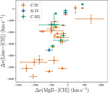
Figure 12. Velocity shifts of the C iv (orange circles), Si iv (blue squares), and C iii] complex peak (green diamonds) with respect to the Mg ii velocity shift. All velocity shifts are measured with respect to the systemic redshift from the [C ii] line. Si iv, C iv, and C iii] are all high-ionization lines, while Mg ii is regarded as a low-ionization line and therefore supposed to originate at a different location in the BLR and under different physical conditions. In addition, the highly blueshifted C iv line is suspected to originate in an outflowing wind. The correlation of the C iv and Mg ii velocity shifts with respect to the [C ii] line redshift potentially indicates a common physical origin of the line velocity shifts.
Download figure:
Standard image High-resolution imageWhile the C iv–Mg ii velocity shifts of our high-redshift quasars show a strong anticorrelation with the C iv FWHM, we do not find an analogous anticorrelation between the Mg ii–[C ii] velocity shift and the Mg ii FWHM (ρ = 0.18, p = 0.36). As Mg ii-based BH masses are based on the assumption that the line traces virialized gas, it is reassuring that the Mg ii FWHM does not correlate with the Mg ii–[C ii] velocity shift (see Figure 14).
The C iii]–[C ii] velocity shifts also show a positive trend with the Mg ii–[C ii] velocity shifts and seem to track the C iv–[C ii] velocity shifts closely. Richards et al. (2011) also noted that the C iii] velocity shifts track the C iv velocity shifts if measured in the same reference system. The authors discuss that the C iii] complex velocity shift is partly due to a relative flux change of the Si iii] and C iii] lines. In their Figure 11 they show that the strength of the Si iii] line increases with C iv blueshift, leading to a stronger velocity blueshift of the entire C iii] complex (see also Shen et al. 2016). Unfortunately, our data did not allow us to resolve the different contributions of the Si iii] and C iii] lines. Hence, we cannot distinguish between real C iii] velocity shifts and the effect of Si iii]-to-C iii] line ratio changes in our sample.
6.2.4. Broad-line Velocity Shifts in Relation to Other Quasar Properties
The presented X-SHOOTER/ALMA quasar sample spans a rather narrow range of high bolometric luminosity ( , with the exception of SDSS J0100+2802). At these luminosities we have measured a large range of C iv–Mg ii velocity shifts (−5000 to 0 km s−1). We have tested whether the continuum luminosity at 3000 Å and the C iv–Mg ii velocity shift are correlated, but we did not find any evidence for it (ρ = 0.015, p = 0.94; see also Figure 15 in Appendix F).
Conversely, previous work on large samples of lower-redshift quasars (Richards et al. 2011; Shen et al. 2016) found significant anticorrelations between the velocity shifts of the high-ionization He ii, Si iv, and C iv lines (with respect to Mg ii) and the quasar luminosity, albeit in lower-luminosity samples and over a larger luminosity range (Shen et al. 2016;  ). These anticorrelations of the velocity shifts with luminosity have been associated with accretion-driven dynamical and/or radiative processes in the BLR that could be responsible for the observed blueshifts (Richards et al. 2011).
The observational bias toward mostly luminous quasars propagates to our observed distribution of Eddington luminosity ratios as calculated from Mg ii-based BH masses. Therefore, our sample shows mostly high Eddington luminosity ratios (0.1 ≲ Lbol/LEdd ≲ a few). Coatman et al. (2016) suggested that quasars with strong C iv–Mg ii blueshifts are indicative of high Eddington luminosity ratios. We do not find any indication for a significant correlation between the C iv–Mg ii, C iv–[C ii], and Mg ii–[C ii] velocity shifts and the Eddington luminosity ratio in our sample. Overall we can summarize that broad lines of luminous high Eddington luminosity ratio quasars exhibit a large range of observed velocity (blue)shifts (see also Mazzucchelli et al. 2017).
Vanden Berk et al. (2001) reported a correlation between ionization potential and line velocity shifts based on their low-redshift composite spectrum of z ∼ 1 SDSS quasars. Based on a deep GNIRS spectrum of ULAS J1342+0928, Onoue et al. (2020) highlighted that the amounts of line blueshifts are proportional to their respective ionization potentials and their values are much larger compared to the Vanden Berk et al. (2001) composite spectrum. In Figure 13 we show Mg ii–[C ii] and C iv–[C ii] velocity shifts for our quasars in comparison to both the Vanden Berk et al. (2001) composite and ULAS J1342+0928 (Onoue et al. 2020). The velocity shifts from our sample span the entire range between the composite spectrum and ULAS J1342+0928.
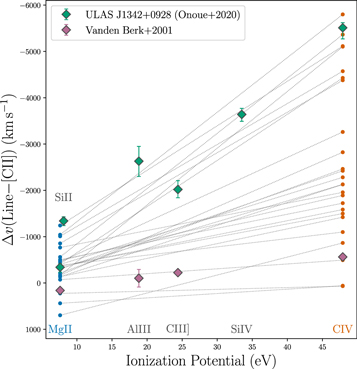
Figure 13. Velocity shifts of emission lines as a function of ionization potential. We only show show Mg ii–[C ii]158μm and C iv–[C ii]158μm velocity shifts of quasars of our sample with filled blue and orange points, respectively. Measurements of the same quasar are connected with a dotted gray line. We compare these measurements with various velocity shifts from ULAS J1342+0928 (Onoue et al. 2020), which were also measured with respect to [C ii]158μm in green. The purple data points show velocity shifts with respect to [O iii] λ5007 from the low-redshift quasar composite of Vanden Berk et al. (2001). Quasars from our sample show a large range of blueshifts.
Download figure:
Standard image High-resolution imageThere are 12 radio-quiet quasars in our high-redshift quasar sample. So far no quasar is confirmed to be radio-loud, while the radio observations are not yet deep enough to classify the remaining 24 objects. Work on low-redshift (z ≤ 1) type 1 AGNs (Sulentic et al. 2007) showed that radio-quiet sources were associated with stronger C iv blueshifts, whereas their sample of radio-loud sources showed C iv velocity shifts around 0 km s−1. Their radio-quiet AGNs also showed a first tentative correlation with C iv blueshift and C iv FWHM not seen in their radio-loud counterparts. We have discussed this correlation in our high-redshift sample (see Figure 10, right panel). Similar trends with radio-loudness were seen in the SDSS quasar sample (Richards et al. 2002), in which radio-loud quasars show on average smaller C iv blueshifts. If the properties of low-redshift AGNs and quasars are any guide, the strong C iv–Mg ii blueshifts in high-redshift quasars go hand in hand with the large observed fraction of radio-quiet objects. However, currently no statistically significant sample of radio-loud objects with NIR spectroscopy at z = 6–7 exists to confirm these correlations with their C iv emission-line properties.
6.2.5. Discussion
The large C iv blueshifts seen in some quasars at lower redshifts emerge as a prominent feature in luminous z ≥ 6 quasar samples. The common interpretation explains these blueshifts in the context of an outflowing, potentially nonvirialized component of the C iv line (e.g., Richards et al. 2002, 2011; Mazzucchelli et al. 2017). This is one reason why the validity of C iv-based BH mass estimates has been scrutinized (e.g., Mejía-Restrepo et al. 2018). Not only does the X-SHOOTER/ALMA sample show a large range of C iv blueshifts, but we also find the Mg ii line, on average, to be blueshifted with respect to the [C ii] emission of the quasar host galaxy. This has been observed in individual objects or small samples at z > 6 (Wang et al. 2016b; Venemans et al. 2016; Mazzucchelli et al. 2017; Onoue et al. 2020) and was recently reported for quasars at z ∼ 4.8 (Nguyen et al. 2020). However, our larger sample size highlights the high frequency of these blueshifts in luminous, reionization-era quasars. Furthermore, we discovered a significant correlation between the C iv–[C ii] and Mg ii–[C ii] velocity shifts, strongly suggesting a common origin likely tied to the physical conditions of the BLR and the accretion process. While we could not find correlations of the velocity shifts with either the quasar's luminosity or Eddington luminosity ratio, such correlations have been observed in lower-redshift samples (Richards et al. 2011). Shen et al. (2016) found the quasar luminosity to be strongly correlated with the He ii, C iv, and Si iv blueshifts, whereas they note that the Mg ii velocity shift is luminosity independent. In their sample of 2 < z < 2.7 quasars Coatman et al. (2016) observed that large C iv blueshifts are associated with high Eddington luminosity ratios. Indeed, studies of very luminous z = 2–4 quasars (WISSH quasar sample; Bischetti et al. 2017; Vietri et al. 2018) find correlations of the C iv blueshift with both bolometric luminosity and Eddington luminosity ratio. As bolometric luminosity and Eddington luminosity ratio are related quantities, the authors conduct a more detailed analysis and conclude that the fundamental variable is the luminosity rather than the Eddington ratio. In addition, they observe a clear correlation between the C iv blueshift and the UV-to-X-ray continuum slope (αOX), as discussed in Richards et al. (2011). Thus, quasars with large C iv blueshifts show a less ionizing spectral energy distribution dominated by UV rather than by X-ray emission. Such a spectrum would naturally be able to produce winds through radiation line driving (Murray et al. 1995).
Let us consider that the broad emission originates from a wind, which emerges from the accretion disk in helical streamlines driven by radiation pressure (Murray et al. 1995). The wind moving toward the observer is responsible for the blueshifted emission, while the receding side is blocked by the optically thick accretion disk. According to this model, the innermost streamlines with gas in the highest ionization states have the largest rotational and radial velocities, which can naturally explain the larger FWHM of C iv with respect to Mg ii, as well as the stratification of the BLR in reverberation mapping observations. The authors also predict that high-ionization lines should be blueshifted relative to low-ionization lines. While this model might have its shortcomings, it offers a compelling picture to explain the observations of the blueshifted quasar emission lines, especially regarding their correlation with ionization potential (Tytler & Fan 1992; McIntosh et al. 1999; Vanden Berk et al. 2001; Onoue et al. 2020).
Emission-line velocity shifts in an axisymmetric wind model naturally open up discussions on orientation measures based on the C iv, Mg ii, and other quasar emission lines (e.g., Richards et al. 2002; Meyer et al. 2019; Yong et al. 2020). However, the complex nature of the BLR and the limited number of observational data sets make it hard to disentangle orientation effects, variations in the physical conditions of the BLR, and biases of the quasar samples.
It is a worthwhile endeavor to expand the presented analysis to quasars at lower redshift and lower luminosities to further investigate the kinematic information provided by emission-line velocity shifts, as they may provide a way to constrain the quasar's orientation.
7. Summary
We presented new and archival X-SHOOTER NIR spectroscopy for 38 quasars at 5.78 < z < 7.54, of which 34 have complimentary [C ii] detection with ALMA. We have discussed the spectral modeling in detail and provide a machine-readable master table online, which includes all measured and derived quantities. An overview of that table is given in Appendix C.
- 1.We have investigated the systematic effects on the Mg ii line and Fe ii pseudocontinuum properties inferred from different iron templates. We specifically compared the VW01 and T06 iron templates. The VW01 template does not include Fe ii emission beneath the Mg ii, whereas the T06 template does. As a consequence, the Mg ii flux and FWHM are overestimated using the VW01 template and the iron contribution is underestimated. Any inclusion of the Fe ii emission beneath the Mg ii line leads to a more realistic estimate of the spectral properties, e.g., for the calculation of the Fe ii/Mg ii flux ratio.
- 2.For estimating SMBH masses, care has to be taken to measure the Mg ii FWHM or σ using the same iron template, which was used to establish the single-epoch virial estimators. We provide a relation that allows us to scale the Fe ii/Mg ii flux ratios as measured with the VW01 template up to measurements with the T06 template.
- 3.We analyzed the Fe ii/Mg ii ratio, a proxy for the BLR iron enrichment for our sample, and found a median value of
 , where uncertainties give the 16th to 84th percentile region. We conclude that the BLRs of all quasars presented in this study are already enriched in iron.
 - 4.We investigated the properties of the broad emission lines with a focus on velocity shifts and the broad C iv and Mg ii lines. We find that high-redshift quasars show a large range of C iv–Mg ii velocity shifts with an emphasis on large blueshifts, which sets them apart from a luminosity-matched sample of 1.52 < z < 2.2 quasars. We calculate a median C iv–Mg ii velocity shift of ∼−1800 km s−1, whereas the low-redshift quasars have a median of ∼−800 km s−1. We further find the Mg ii line to be often blueshifted with respect to the [C ii] of the host galaxy measured with ALMA. The velocity shift distribution shows a clear peak around the median,.
- 5.We find the velocity shifts of C iv and Mg ii, both with respect to the host galaxy [C ii] line, to be significantly correlated, indicating a common origin likely tied to the physical properties of the BLR and the accretion process.
- 6.We did not find evidence for correlations between between the line velocity shifts and the bolometric luminosity or the Eddington ratio, keeping in mind that our sample is dominated by luminous, high Eddington luminosity ratio quasars.
![${\rm{\Delta }}v(\mathrm{MgII}-[\mathrm{CII}])=-{390.61}_{-455.34}^{256.02}\,\mathrm{km}\,{{\rm{s}}}^{-1}$](https://content.cld.iop.org/journals/0004-637X/905/1/51/revision1/apjabc2d7ieqn492.gif)
7.1. Do Quasar Emission-line Properties Evolve with Redshift?
As we discover more and more high-redshift quasars deep within the era of reionization, it would not be surprising if we saw their emission-line properties evolve. Yet quasar spectra at z ∼ 6 bear surprising resemblance to their low-redshift (z ≈ 1–2) counterparts (Shen et al. 2019b). Probing quasars at even higher redshifts than Shen et al. (2019b), our analysis takes a close look at the C iv and Mg ii lines, as well as the Fe ii contribution. As seen from Figure 7, our median Fe ii/Mg ii flux ratio agrees well with measurements at lower redshifts (z = 3–5), showing no significant redshift evolution. In Figure 11 our data show significant blueshifts between the measurements of the Mg ii–[C ii] lines. Yet this is also not unique to z ≳ 6 quasars, as similar results are found at z ∼ 4.8 (Nguyen et al. 2020). Many quasars in our sample also show large C iv–Mg ii velocity blueshifts (Δv(CIV − Mgii) < −2000 km s−1) that correlate with smaller C iv EW and larger C iv FWHM (see Figure 10). Judging from this figure, we can always identify low-redshift (z = 1.52–2.2) quasars occupying the same region of the C iv–Mg ii/EW or the C iv–Mg ii/FWHM parameter space. However, the average sample C iv–Mg ii velocity shift does seem to decrease significantly at the highest redshifts (Figure 9). This trend, first reported and discussed in Meyer et al. (2019), is supported by our analysis on a larger high-redshift sample. Yet it is unclear whether this apparent redshift evolution presents a physical change in the BLR conditions or a selection bias affecting the highest-redshift quasars. The advent of the James Webb Space Telescope will open up possibilities to probe the rest-frame optical emission of high-redshift quasars, providing access to the hydrogen Balmer lines. These measurements will be instrumental for a comprehensive comparison of high-redshift quasars with the low-redshift quasar population.
The authors thank R. Meyer for providing line redshifts with improved accuracy for the "z6" and "z7" quasar samples in Meyer et al. (2019). J.Y. and X.F. acknowledge the support from the NASA ADAP grant NNX17AF28G. A.C.E. acknowledges support by NASA through the NASA Hubble Fellowship grant No. HF2-51434 awarded by the Space Telescope Science Institute, which is operated by the Association of Universities for Research in Astronomy, Inc., for NASA, under contract NAS5-26555. F.W. acknowledges support provided by NASA through the NASA Hubble Fellowship grant No. HST-HF2-51448.001-A awarded by the Space Telescope Science Institute, which is operated by the Association of Universities for Research in Astronomy, Incorporated, under NASA contract NAS5-26555.
Facility: VLT:Kueyen (X-SHOOTER). -
Software: Astropy (Astropy Collaboration et al. 2013, 2018), SciPy (Virtanen et al. 2020), Numpy (van der Walt et al. 2011; Harris et al. 2020), Pandas (pandas development team 2020; McKinney 2010), LMFIT (Newville et al. 2014), Pypeit (Prochaska et al. 2019, 2020), Extinction (Barbary 2016).
Appendix A: Additional Tables
We present additional tables detailing further properties of the X-SHOOTER/ALMA sample in this section. Table 7 includes measurements on the C iii] and Si iv lines, and Table 8 summarizes additional information on the quasar fits, their continuum measurements, and information on classifications.
Table 7. Properties of the C iii] and Si iv Emission Lines
| Quasar Name | zCIII] | Δv(CIII] − [Cii]) | zSiIV | FWHMSiIV | EWSiIV | Δv(SiIV − [Cii]) |
|---|---|---|---|---|---|---|
| (km s−1) | (km s−1) | (Å) | (km s−1) | |||
| PSO J004.3936+17.0862 |

|

|
⋯ | ⋯ | ⋯ | ⋯ |
| PSO J007.0273+04.9571 |

|

|
⋯ | ⋯ | ⋯ | ⋯ |
| PSO J009.7355–10.4316 | ⋯ | ⋯ | ⋯ | ⋯ | ⋯ | ⋯ |
| PSO J011.3898+09.0324 | ⋯ | ⋯ | ⋯ | ⋯ | ⋯ | ⋯ |
| VIK J0046–2837 | ⋯ | ⋯ | ⋯ | ⋯ | ⋯ | ⋯ |
| SDSS J0100+2802 | ⋯ | ⋯ | ⋯ | ⋯ | ⋯ | ⋯ |
| VIK J0109–3047 | ⋯ | ⋯ | ⋯ | ⋯ | ⋯ | ⋯ |
| PSO J036.5078+03.0498 | ⋯ | ⋯ |

|

|

|

|
| VIK J0305–3150 | ⋯ | ⋯ | ⋯ | ⋯ | ⋯ | ⋯ |
| PSO J056.7168–16.4769 |

|

|
⋯ | ⋯ | ⋯ | ⋯ |
| PSO J065.4085–26.9543 | ⋯ | ⋯ | ⋯ | ⋯ | ⋯ | ⋯ |
| PSO J065.5041–19.4579 | ⋯ | ⋯ | ⋯ | ⋯ | ⋯ | ⋯ |
| SDSS J0842+1218 | ⋯ | ⋯ | ⋯ | ⋯ | ⋯ | ⋯ |
| SDSS J1030+0524 | ⋯ | ⋯ | ⋯ | ⋯ | ⋯ | ⋯ |
| PSO J158.69378–14.42107 | ⋯ | ⋯ | ⋯ | ⋯ | ⋯ | ⋯ |
| PSO J159.2257–02.5438 | ⋯ | ⋯ | ⋯ | ⋯ | ⋯ | ⋯ |
| SDSS J1044–0125 |

|

|
⋯ | ⋯ | ⋯ | ⋯ |
| VIK J1048–0109 | ⋯ | ⋯ | ⋯ | ⋯ | ⋯ | ⋯ |
| ULAS J1120+0641 |

|

|

|

|

|

|
| ULAS J1148+0702 | ⋯ | ⋯ | ⋯ | ⋯ | ⋯ | ⋯ |
| PSO J183.1124+05.0926 | ⋯ | ⋯ | ⋯ | ⋯ | ⋯ | ⋯ |
| SDSS J1306+0356 |

|

|
⋯ | ⋯ | ⋯ | ⋯ |
| ULAS J1319+0950 |

|

|
⋯ | ⋯ | ⋯ | ⋯ |
| ULAS J1342+0928 |

|

|

|

|

|

|
| CFHQS J1509–1749 |

|

|
⋯ | ⋯ | ⋯ | ⋯ |
| PSO J231.6576–20.8335 | ⋯ | ⋯ | ⋯ | ⋯ | ⋯ | ⋯ |
| PSO J239.7124–07.4026 | ⋯ | ⋯ | ⋯ | ⋯ | ⋯ | ⋯ |
| PSO J308.0416–21.2339 | ⋯ | ⋯ | ⋯ | ⋯ | ⋯ | ⋯ |
| SDSS J2054–0005 |

|

|
⋯ | ⋯ | ⋯ | ⋯ |
| CFHQS J2100–1715 | ⋯ | ⋯ | ⋯ | ⋯ | ⋯ | ⋯ |
| PSO J323.1382+12.2986 |

|

|

|

|

|

|
| VIK J2211–3206 | ⋯ | ⋯ | ⋯ | ⋯ | ⋯ | ⋯ |
| CFHQS J2229+1457 | ⋯ | ⋯ | ⋯ | ⋯ | ⋯ | ⋯ |
| PSO J340.2041–18.6621 |

|

|
⋯ | ⋯ | ⋯ | ⋯ |
| SDSS J2310+1855 | ⋯ | ⋯ | ⋯ | ⋯ | ⋯ | ⋯ |
| VIK J2318–3029 | ⋯ | ⋯ | ⋯ | ⋯ | ⋯ | ⋯ |
| VIK J2348–3054 |

|

|
⋯ | ⋯ | ⋯ | ⋯ |
| PSO J359.1352–06.3831 | ⋯ | ⋯ | ⋯ | ⋯ | ⋯ | ⋯ |
Table 8. Additional Properties of the X-SHOOTER/ALMA Quasar Sample
| Quasar Name | Classification | Class. Reference | Power-law Slope | M1450 | L1450 | L3000 | Lbol |
|---|---|---|---|---|---|---|---|
| (AB mag) | (1046 erg s−1) | ||||||
| PSO J004.3936+17.0862 | Y | f, This work |

|

|

|

|

|
| PSO J007.0273+04.9571 | ⋯ | ⋯ |

|

|

|

|

|
| PSO J009.7355–10.4316 | D | This work | ⋯ |

|

|

|

|
| PSO J011.3898+09.0324 | ⋯ | ⋯ |

|

|

|

|

|
| VIK J0046–2837 | D | This work | ⋯ |

|

|

|

|
| SDSS J0100+2802 | Y | b |

|

|

|

|

|
| VIK J0109–3047 | ⋯ | ⋯ |

|

|

|

|

|
| PSO J036.5078+03.0498 | ⋯ | ⋯ |

|

|

|

|

|
| VIK J0305–3150 | ⋯ | ⋯ |

|

|

|

|

|
| PSO J056.7168–16.4769 | pDLA | f, g |

|

|

|

|

|
| PSO J065.4085–26.9543 | D | This work | ⋯ |

|

|

|

|
| PSO J065.5041–19.4579 | BAL, D | This work | ⋯ |

|

|

|

|
| SDSS J0842+1218 | ⋯ | ⋯ |

|

|

|

|

|
| SDSS J1030+0524 | ⋯ | ⋯ |

|

|

|

|

|
| PSO J158.69378–14.42107 | Y | f |

|

|

|

|

|
| PSO J159.2257–02.5438 | ⋯ | ⋯ |

|

|

|

|

|
| SDSS J1044–0125 | BAL | d |

|

|

|

|

|
| VIK J1048–0109 | ⋯ | ⋯ |

|

|

|

|

|
| ULAS J1120+0641 | ⋯ | ⋯ |

|

|

|

|

|
| ULAS J1148+0702 | ⋯ | ⋯ |

|

|

|

|

|
| PSO J183.1124+05.0926 | pDLA | e |

|

|

|

|

|
| SDSS J1306+0356 | ⋯ | ⋯ |

|

|

|

|

|
| ULAS J1319+0950 | ⋯ | ⋯ |

|

|

|

|

|
| ULAS J1342+0928 | ⋯ | ⋯ |

|

|

|

|

|
| CFHQS J1509–1749 | ⋯ | ⋯ |

|

|

|

|

|
| PSO J231.6576–20.8335 | ⋯ | ⋯ |

|

|

|

|

|
| PSO J239.7124–07.4026 | BAL | f |

|

|

|

|

|
| PSO J308.0416–21.2339 | ⋯ | ⋯ |

|

|

|

|

|
| SDSS J2054–0005 | ⋯ | ⋯ |

|

|

|

|

|
| CFHQS J2100–1715 | Y, D | f, This work | ⋯ |

|

|

|

|
| PSO J323.1382+12.2986 | ⋯ | ⋯ |

|

|

|

|

|
| VIK J2211–3206 | BAL | This work |

|

|

|

|

|
| CFHQS J2229+1457 | ⋯ | ⋯ |

|

|

|

|

|
| PSO J340.2041–18.6621 | BAL | This work |

|

|

|

|

|
| SDSS J2310+1855 | pDLA | c |

|

|

|

|

|
| VIK J2318–3029 | ⋯ | ⋯ |

|

|

|

|

|
| VIK J2348–3054 | BAL | a |

|

|

|

|

|
| PSO J359.1352–06.3831 | ⋯ | ⋯ |

|

|

|

|

|
References.—Quasar classification: broad absorption line quasar (BAL), proximate damped Lyman-alpha absorber (pDLA), young quasars (Y), quasar continuum not described by power law (D). The classification references are: a = De Rosa et al. (2014), b = Eilers et al. (2017), c = D'Odorico et al. (2018), d = Shen et al. (2019b), e = Bañados et al. (2019a), f = Eilers et al. (2020), g = Davies (2020).
Appendix B: Notes on the Spectral Modeling of Individual Quasars
In this appendix we provide additional information on the model fits of individual quasars. As the redshift and the S/N of the X-SHOOTER spectrum vary from object to object, additional assumptions and limitations were necessary to provide an adequate fit.
For example, in a range of spectra we do not use the fit weights, which are taken to be the squared inverse flux uncertainties, for the continuum model. In these spectra the continuum fit was dominated by higher S/N in the continuum regions around the Mg ii line. As a consequence, the continuum around the C iv line was not properly fit. Disabling the fit weights for the continuum allowed for a proper fit of the continuum model.
An overview of which lines were modeled in each quasar is provided in Table 1. In the table we also indicate, in parentheses, in which quasars the C iv emission line was fit with only one Gaussian component (1G) instead of two.
B.1.1. PSO J004.3936+17.0862
In the spectrum of this quasar the Mg ii line falls into one of the telluric absorption bands. To properly fit the continuum, including the iron contribution, we have assumed an FWHM for the iron template of FWHMFeII = 2500 km s−1 and set the Fe ii redshift to the systemic redshift. The low S/N of this spectrum did not justify using more than one Gaussian component to model the C iv line.
B.2. PSO J007.0273+04.9571
To properly fit the continuum over the entire observed wavelength range, we disabled the fit weights for the continuum model. While we do fit the C iii] line complex, the redward part of the C iii] line falls into a window of strong telluric absorption. We caution against overinterpreting the resulting C iii] properties in this case.
B.3. PSO J009.7355–10.4316
This quasar has especially weak lines, and the continuum does not resemble a power-law shape. Hence, we approximated the continuum around the C iv line with a simple power law and fit the line with one Gaussian profile. The Mg ii line lies very close to one telluric absorption band, and model fits were not able to constrain the line properties.
B.4. PSO J011.3898+09.0324
This quasar has a relatively low S/N, allowing us to fit the C iv with one Gaussian component only.
B.5. VIK J0046–2837
This quasar has especially weak lines, and the continuum does not resemble a power-law shape. We approximated the continuum around the Mg ii line with a simple power law and fit for the line. The low S/N in the J band did not allow us to constrain the properties of C iv or C iii] line.
B.6. SDSS J0100+2802
This spectrum has a high S/N. As a consequence, the monolithic iron template around the Mg ii line (2200–3500 Å) was not able to properly model the continuum. Therefore, we divided the iron template into three regions similar to those of Tsuzuki et al. (2006) (2200–2660 Å, 2660–3000 Å, 3000–3500 Å) and modeled their amplitudes separately. Furthermore, the telluric correction algorithm was not able to fully correct the region around the C iv line (11000–11600 Å). This strongly affects any attempts to model the C iv line, and we decided against including a C iv line model.
B.7. VIK J0109–3047
Even though the redshift of this quasar would allow us to fit the C iii] complex, we cannot securely constrain the model owing to the low S/N of the spectrum. Hence, we only fit the C iv and Mg ii, modeling C iv with one Gaussian component.
B.8. PSO J036.5078+03.0498
We have included an Si iv line model (single Gaussian component) for this fit and modeled the C iv with one Gaussian component only.
B.9. VIK J0305–3150
While the redshift of this quasar would allow us to include the Si iv line in the fit, the shape of the spectrum deviates from a power law blueward of the C iv line. Hence, the Si iv line was not included in our fit. The C iv line was modeled with a single Gaussian component.
B.10. PSO J056.7168–16.4769
This spectrum has a relatively high S/N, which allowed us to fit the C iv, C iii], and Mg ii lines.
B.11. PSO J065.4085–26.9543
The continuum strongly deviates from a power-law shape. We approximated the continuum around the Mg ii and C iv lines and fit them separately with individual continuum models. The C iv line is rather broad in this spectrum and shows a broad redward absorption feature that might well be the result of a poor telluric correction in the 11000–11600 Å region. We fit the C iv line using a single Gaussian component and caution against overinterpreting the fit results.
B.12. PSO J065.5041–19.4579
In the spectrum of this quasar the continuum strongly deviates from a power-law shape. We approximated the continuum around the Mg ii and C iv lines and fit them separately with individual continuum models. The C iv line is partially absorbed by a strong blueward absorption trough. Thus, we restricted the line fit to the redward half of the line and approximated the C iv line using only one Gaussian component.
B.13. SDSS J0842+1218
In order to properly fit the continuum over the entire wavelength range, it was necessary to disable the fit weights for the continuum model. The blueward wing of the C iii] complex is outside of the telluric absorption band, but its peak is not. Therefore, any line fit would be associated with high uncertainties, and we decided against modeling of the C iii] in this quasar.
B.14. PSO J158.69378–14.42107
To properly fit the continuum over the entire wavelength range, it was necessary to disable the fit weights for the continuum model.
B.15. SDSS J1044–0125
To properly fit the continuum over the entire wavelength range, it was necessary to disable the fit weights for the continuum model. In this spectrum the Mg ii line falls into one of the telluric absorption bands. To properly fit the continuum, including the iron contribution, we have assumed an FWHM for the iron template of FWHMFeII = 2500 km s−1 and set the Fe ii redshift to the systemic redshift of the quasar. The C iv line is partially absorbed by a strong blueward absorption trough. Thus, we restricted the line fit to the redward half of the line and approximated the C iv line using only one Gaussian component. The C iii] complex has a very broad structure in this spectrum.
B.16. VIK J1048–0109
The overall low S/N of this spectrum did not allow us to model the C iv line.
B.17. ULAS J1120+0641
Unfortunately, the Mg ii line of this spectrum falls in the gap between the last two orders of the X-SHOOTER spectrograph. Due to the faint nature of the quasar, the extracted traces of the last orders do not overlap and strong artifacts plague the echelle order boundary. Hence, we were unable to fit the Mg ii line. To properly fit the continuum, including the iron contribution, we have assumed an FWHM for the iron template of FWHMFeII = 2500 km s−1 and set the Fe ii redshift to the systemic redshift of the quasar. The high redshift of this quasar allows us to successfully model the Si iv line (single Gaussian component), as well as the C iii] complex.
B.18. PSO J183.1124+05.0926
In this spectrum the C iv line falls into the wavelength range of 11000–11600 Å, where either telluric absorption features could not be fully corrected or intrinsic absorption is present. We further see absorption in the profile of the Mg ii line. We exclude the worst residuals from both the C iv and Mg ii line fits and approximate the C iv line using only one Gaussian component.
B.19. SDSS J1306+0356
To properly fit the continuum over the entire range, it was necessary to disable the fit weights for the continuum model.
B.20. ULAS J1319+0950
While we have included the C iii] complex in the fit, we would like to caution against overinterpreting its fit results, as it partially falls in a region of strong telluric absorption. In addition, our best fits seems to overpredict the Fe ii pseudocontinuum redward of the Mg ii line.
B.21. ULAS J1342+0928
The Mg ii line is not detected in this spectrum, as it falls close to the red edge of the last echelle order, which is dominated by noise. However, we are able to include the Si iv line in our model. Due to the extremely broad nature of the Si iv and C iv lines, both were modeled using only a single Gaussian component each.
B.22. CFHQS J1509–1749
To properly fit the continuum over the entire range, it was necessary to disable the fit weights for the continuum model. Additionally, the C iii] complex falls partly in a region of strong telluric absorption, and therefore we caution against overinterpreting the resulting C iii] properties in this case.
B.23. PSO J231.6576–20.8335
The low S/N of this spectrum did not allow us to model the C iv line successfully.
B.24. PSO J239.7124–07.4026
To properly fit the continuum over the entire range, it was necessary to disable the fit weights for the continuum model.
B.25. SDSS J2054–0005
To properly fit the continuum over the entire range, it was necessary to disable the fit weights for the continuum model. The low S/N of this spectrum did not justify using more than one Gaussian component to model the C iv line. For the same reason we set the contribution of the Si iii] line to the C iii] complex to zero.
B.26. CFHQS J2100–1715
The low S/N of this spectrum did not justify using more than one Gaussian component to model the C iv line.
B.27. PSO J323.1382+12.2986
The higher redshift of this quasar allows us to successfully model the Si iv line with a single Gaussian component. The C iii] complex falls partially in one of the bands of strong telluric absorption. As a consequence, we set the contribution of the Al iii line to the C iii] complex to zero and caution against overinterpreting the C iii] complex properties with the exception of the peak redshift.
B.28. VIK J2211–3206
In this spectrum the C iv line falls into the wavelength range of 11000–11600 Å, where telluric absorption features could not be fully corrected. We exclude the worst residuals from the line fit and approximate the C iv line using only a single Gaussian component. We also note that a strong absorption feature blueward of the C iv line complicates the modeling. Hence, we have excluded part of this region from the fit for the line.
B.29. CFHQS J2229+1457
The low-S/N spectrum did not allow us to constrain the Mg ii with a fit. The strong C iv emission was modeled with two Gaussian components.
B.30. PSO J340.2041–18.6621
The C iv line and the C iii] complex show strong absorption features within their profiles, which have been excluded from the fit. While we have included the C iii] complex in the fit, we would like to caution against overinterpreting its fit results, as the complex partially falls in a region of strong telluric absorption.
B.31. SDSS J2310+1855
The C iv line and the C iii] line are unusually broad in this spectrum. In addition, the blue edge of the C iv line is affected either by the declining throughput at the blue edge of the spectrum or by absorption. Therefore, we decided to model the C iv line with only a single Gaussian component and exclude the C iii] complex from the fit. To properly fit the continuum over the entire wavelength range, it was necessary to disable the fit weights for the continuum model.
B.32. VIK J2318–3029
To properly fit the continuum over the entire range, it was necessary to disable the fit weights for the continuum model. Absorption features within the C iv line were masked for the fit.
B.33. VIK J2348–3054
The C iv line is partially absorbed by a strong blueward absorption trough. Thus, we restricted the line fit to the redward half of the line and approximated the C iv line using only a single Gaussian component. To properly fit the C iii] complex, we mask a strong absorption doublet in its center.
B.34. PSO J359.1352–06.3831
In the spectrum of this quasar the Mg ii line falls into a region of strong residuals from telluric absorption features (19900–20200 Å), potentially biasing the derived line properties. We mask out the strongest feature for the fit.
Appendix C: The X-SHOOTER/ALMA Master Table
The X-SHOOTER/ALMA master table of the NIR spectral analysis is available as a machine-readable table online. It has 175 columns, detailed in Table 9 below. For all fit properties we provide the median (_med) value, as well as the differences from the median to the 16th (_low) and 84th (_upp) percentile values. Hence, each fit property has three columns in the table. The shorthand VW01 refers to fit properties derived from fits with the VW01 iron template. All other fit properties were derived using the T06 iron template.
Table 9. Description of the Online-only Master Table of the X-SHOOTER/ALMA Sample of Quasars in the Epoch of Reionization
| Column | Name | Unit | Description |
|---|---|---|---|
| 1 | Name | ⋯ | Quasar name |
| 2 | Zsys | ⋯ | Systemic redshift |
| 3 | Zsys_e | ⋯ | Systemic redshift error |
| 4 | Z_method | ⋯ | Method for systemic redshift |
| 5 | z_ref | ⋯ | Reference for systemic redshift |
| 6 | RA | decimal degrees | Right ascension |
| 7 | Decl | decimal degrees | decl. |
| 8 | J | AB mag | J-band magnitude |
| 9 | Je | AB mag | J-band magnitude error |
| 10 | disk_ref | ⋯ | Discovery reference |
| 11–13 | flux_1350 | 10−17 erg s−1 cm−2 Å−1 | Continuum model flux at 1350 Å |
| 14–16 | L_1350 | 1046 erg s−1 | Continuum model luminosity at 1350 Å |
| 17–19 | flux_1450 | 10−17 erg s−1 cm−2 Å−1 | Continuum model flux at 1450 Å |
| 20–22 | L_1450 | 1046 erg s−1 | Continuum model luminosity at 1450 Å |
| 23–25 | flux_2500 | 10−17 erg s−1 cm−2 Å−1 | Continuum model flux at 2500 Å |
| 26–28 | L_2500 | 1046 erg s−1 | Continuum model luminosity at 2500 Å |
| 29–31 | flux_3000 | 10−17 erg s−1 cm−2 Å−1 | Continuum model flux at 3000 Å |
| 32–34 | L_3000 | 1046 erg s−1 | Continuum model luminosity at 3000 Å |
| 35–37 | Lbol | 1046 erg s−1 | Bolometric luminosity |
| 38–40 | m1450 | AB mag | Apparent magnitude at 1450 Å |
| 41–43 | M1450 | AB mag | Absolute magnitude at 1450 Å |
| 44–46 | Plslope | ⋯ | Continuum model power-law slope |
| 47–49 | CIV_wav_cen | Å | C iv peak wavelength |
| 50–52 | CIV_z_cen | ⋯ | C iv peak redshift |
| 53–55 | CIV_vshift | km s−1 | C iv velocity shift to Zsys |
| 56–58 | CIV_FWHM | km s−1 | C iv FWHM |
| 59–61 | CIV_EW | Å | C iv rest-frame EW |
| 62–64 | CIV_FWHM_corr | km s−1 | C iv corrected FWHM (Coatman et al. 2017) |
| 65–67 | CIV_flux | erg s−1 cm−2 Å−1 | Integrated C iv flux |
| 68–70 | CIV_L | erg s−1 | Integrated C iv luminosity |
| 71–73 | CIV_BHM_V06 | 109 M⊙ | C iv BH mass (Vestergaard & Peterson 2006) |
| 74–76 | CIV_EddR_V06 | ⋯ | C iv Eddington luminosity ratio (Vestergaard & Peterson 2006) |
| 77–79 | CIV_BHM_Co17 | 109 M⊙ | C iv BH mass (Coatman et al. 2017) |
| 80–82 | CIV_EddR_Co17 | ⋯ | Mg ii Eddington luminosity ratio (Coatman et al. 2017) |
| 83–85 | MgII_wav_cen | Å | Mg ii peak wavelength |
| 86–88 | MgII_z_cen | ⋯ | Mg ii peak redshift |
| 89–91 | MgII_vshift | km s−1 | Mg ii velocity shift to Zsys |
| 92–94 | MgII_FWHM | km s−1 | Mg ii FWHM |
| 95–97 | MgII_EW | Å | Mg ii rest-frame EW |
| 98–100 | MgII_flux | erg s−1 cm−2 Å−1 | Integrated Mg ii flux |
| 101–103 | MgII_L | erg s−1 | Integrated Mg ii luminosity |
| 104–106 | FeII_flux | erg s−1 cm−2 Å−1 | Integrated Fe ii flux |
| 107–109 | FeIIMgII_ratio | ⋯ | Fe ii/Mg ii flux ratio |
| 110–112 | CIII_z | ⋯ | C iii] complex model redshift |
| 113–115 | CIII_vshift | km s−1 | C iii] complex peak velocity shift to Zsys |
| 116–118 | SiIV_wav_cen | Å | Si iv peak wavelength |
| 119–121 | SiIV_z_cen | ⋯ | Si iv peak redshift |
| 122–124 | SiIV_vshift | km s−1 | Si iv velocity shift to Zsys |
| 125–127 | SiIV_FWHM | km s−1 | Si iv FWHM |
| 128–130 | SiIV_EW | Å | Si iv rest-frame EW |
| 131–133 | SiIV_flux | erg s−1 cm−2 Å−1 | Integrated Si iv flux |
| 134–136 | SiIV_L | erg s−1 | Integrated Si iv luminosity |
| 137–139 | VW01_MgII_wav_cen | Å | Mg ii peak wavelength |
| 140–142 | VW01_MgII_z_cen | ⋯ | Mg ii peak redshift |
| 143–145 | VW01_MgII_vshift | km s−1 | Mg ii velocity shift to Zsys |
| 146–148 | VW01_MgII_FWHM | km s−1 | Mg ii FWHM |
| 149–151 | VW01_MgII_EW | Å | Mg ii rest-frame EW |
| 152–154 | VW01_MgII_flux | erg s−1 cm−2 Å−1 | Integrated Mg ii flux |
| 155–157 | VW01_MgII_L | erg s−1 | Integrated Mg ii luminosity |
| 158–160 | VW01_MgII_BHM_VW09 | 109 M⊙ | Mg ii BH mass (Vestergaard & Osmer 2009) |
| 161–163 | VW01_MgII_EddR_VW09 | ⋯ | Mg ii Eddington luminosity ratio (Vestergaard & Osmer 2009) |
| 164–166 | VW01_MgII_BHM_S11 | 109 M⊙ | Mg ii BH mass (Shen et al. 2011) |
| 167–169 | VW01_MgII_EddR_S11 | ⋯ | Mg ii Eddington luminosity ratio (Shen et al. 2011) |
| 170 | Resolution | ⋯ | Lowest resolution of all used observations |
| 171 | Exptime | s | Total exposure time |
| 172 | ProgramIDs | ⋯ | ESO proposal program IDs |
| 173 | PIs | ⋯ | Principal Investigators |
| 174 | S/N_J | ⋯ | Mean S/N over 12500–13450 Å |
| 175 | S/N_J_binned | ⋯ | Mean S/N over 12500–13450 Å (binned) |
Only a portion of this table is shown here to demonstrate its form and content. A machine-readable version of the full table is available.
Appendix D: Derivation of the BH Masses
In this appendix we briefly discuss the calculation of our BH mass estimates. The derived BH masses are then presented and further discussed in E. P. Farina et al. (2020, in preparation).
The properties of the broad emission lines, probes of the BLR gas, allow for first-order estimates. Under the assumption that the line-emitting gas is in virial motion (e.g., a disk with Keplerian rotation) around the SMBH, the line-of-sight velocity dispersion of the gas, measured as the FWHM of the broad emission line (FWHMBLR), traces the gravitational potential of the SMBH mass (MBH):
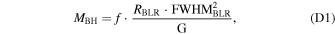
where RBLR denotes the radius from the SMBH to the line-emitting region for the particular emission line in question. Here the factor f encapsulates our ignorance on orientation, structure, and more complex kinematics of the BLR. While it is generally assumed to be of order unity (Peterson et al. 2004; Decarli et al. 2010; Mediavilla et al. 2020), it gives rise to significant systematic uncertainties (e.g., Krolik 2001). Reverberation mapping campaigns have found a strong correlation between RBLR and the quasar's continuum luminosity (e.g., Kaspi et al. 2000, 2005; Bentz et al. 2013) and been successful in measuring BH masses (e.g., Onken et al. 2004; Peterson et al. 2004). These results have been recently supported by spatially resolved observations of the BLR in 3C 273 (Gravity Collaboration et al. 2018). Based on the reverberation mapping results, scaling relations have been derived, which allow us to estimate a quasar's BH mass solely based on the velocity dispersion of a broad line and its continuum luminosity. These so-called single-epoch virial mass estimators allow us to estimate the BH mass of a quasar based on a single spectrum and are often written as
The zero-points zp and the parameter b depend on the broad emission line in question and the monochromatic continuum luminosity Lλ,x at a given rest-frame wavelength x. Single-epoch virial BH mass estimates have a considerable systematic uncertainty due to the unknowns encompassed in the f factor, which surface as scatter in the radius–luminosity relations. These systematic uncertainties can be as large as ∼0.55 dex (Vestergaard & Osmer 2009). We derive BH mass estimates from the properties of the broad Mg ii and C iv emission lines and the adjacent continuum.
Mg ii: For the Mg ii line we adopt the single-epoch virial mass estimators of Vestergaard & Osmer (2009, zp = 6.86, b = 0.5, x = 3000 Å) and (Shen et al. 2011, zp = 6.74, b = 0.62, x = 3000 Å). The scaling relation of Vestergaard & Osmer (2009) uses single or multiple Gaussian components to model and measure the FWHM of the Mg ii. In the cases of a multicomponent model the FWHM is calculated from the full-line model. The scaling relation of Shen et al. (2011) uses the radius–luminosity relationship of McLure & Dunlop (2004) and recalibrates the zero-point to the Hβ relation of Vestergaard & Peterson (2006). The FWHM of Mg ii is always determined with multiple components, with at least a narrow and a broad component both modeled with Gaussian profiles. While the S/N in our spectra does not justify a multicomponent fit for Mg ii, we still argue that both scaling relations are valid in our case as long as the emission line is properly represented by our fit.
We model the FWHM of the Mg ii line for BH mass estimates from both relations using the VW01 iron template for the Fe ii continuum. As we discuss in Section 5, the modeling of the iron pseudocontinuum introduces systematic effects on the measured FWHM of the Mg ii line. Therefore, our BH mass estimates are based on the FWHM determinations using the VW01 iron template analogous to the determinations of the scaling relations.
C iv: Contrary to lower-ionization lines, such as Hβ or Mg ii, the C iv emission line often shows highly asymmetric line profiles correlating with the quasar's luminosity and that are commonly associated with an outflowing wind component (e.g., Richards et al. 2011). Outflows that can possibly manifest as a nonreverberating component (Denney 2012) can significantly bias BH mass measurements based on C iv single-epoch virial estimators. Hence, extensive discussions (e.g., Shen 2013; Coatman et al. 2016; Mejía-Restrepo et al. 2018) revolve around the reliability of C iv-based BH masses and corrections for these biases (e.g., Denney 2012; Park et al. 2013; Runnoe et al. 2013; Mejía-Restrepo et al. 2016; Coatman et al. 2017; Zuo et al. 2020).
For a few quasars in our sample the Mg ii line could not be measured, as it falls into a region with extremely low S/N. In most cases these are telluric absorption regions of the reddest order of the X-SHOOTER NIR spectrum. Thus, we decided to use the C iv line to determine BH masses in these cases. We adopt the scaling relation of Vestergaard & Peterson (2006, zp = 6.66, b = 0.53, x = 1350 Å) and correct the BH masses according to Equations (4) and (6) of Coatman et al. (2017). While our measurement of the C iv line properties can be considered equivalent to Vestergaard & Peterson (2006), Coatman et al. (2017) modeled the C iv line with Gauss–Hermite polynomials. We judge the uncertainties introduced by the different fitting methodology likely to be small compared to the systematic uncertainty on the BH mass estimate itself. For their correction Coatman et al. (2017) measured the velocity blueshift from the C iv model centroid with respect to the Hα Balmer line, which is considered a good proxy of the systemic redshift of the quasar. Instead of the Hα line, we have used the systemic redshifts provided in Table 1 to derive the C iv blueshifts.
Appendix E: Construction of the Low-z Comparison Sample
The low-redshift comparison sample is constructed from the catalog of SDSS DR7 quasars published by Shen et al. (2011) using the updated redshift from Hewett & Wild (2010) 16
(see also Wild & Hewett 2005). We select a subsample of quasars broadly following Richards et al. (2011) and Mazzucchelli et al. (2017) to retrieve objects with secure C iv and Mg ii measurements. We only consider quasars in the redshift range 1.52 ≤ z ≤ 2.2, where both emission lines are covered by the SDSS spectrograph. We require the C iv and Mg ii line to be well detected: FWHMCIV > 1000 and FWHMCIV > 2σFWHM,CIV and EWCIV > 5 Å and EWCIV > 2σEW,CIV and FWHMMgII > 1000 and FWHMMgII > 2σFWHM,MgII and EWMgII > 2σEW,MgII. Additionally, we only consider quasars without BALs (BAL_FLAG == 0) and with valid C iv and Mg ii velocity shifts (VOFF_CIV_PEAK < 20000 and VOFF_BROAD_MGII < 20000) measured in relation to their systemic redshifts based on the SDSS pipeline (Stoughton et al. 2002). We have confirmed that the FWHMCIV > 1000 and FWHMMgII > 1000 criteria, which are responsible for removing ∼1% of the spectra, do not remove well-measured narrow lines. In the large majority of cases we find FWHM = 0 in the catalog. In the few cases where the catalog reports a nonzero FWHM, our visual inspection found that the automated model fits have failed. This subset was matched to the updated redshifts of Hewett & Wild (2010) to form a sample of 20,239 quasars. Finally, we further limit the low-redshift sample to a similar bolometric luminosity range for a fair comparison with our high-redshift quasars ( ). This reduces the low-redshift sample to 12,099, which we will use for comparison throughout Section 6.2.
Appendix F: Additional Figures of Broad Emission Line Properties
In this appendix we present additional figures showing broad emission-line properties. Figure 14 shows the Mg ii FWHM as a function of the Mg ii–[C ii] velocity shift. Figure 15 shows the luminosity at 3000 Å as a function of the C iv–Mg ii velocity shift. There is no indication for any correlations in both of the figures. Lastly, in Figure 16 we show the Mg ii–[C ii], Mg ii-C iv, and C iv–Mg ii velocity shifts as a function of the Eddington luminosity ratio. The Eddington luminosity ratio was determined from the Mg ii line using the Vestergaard & Osmer (2009) relation to the FWHM measured with the VW01 iron template. We tested for correlations and found none of the velocity shifts to be correlated with the Eddington luminosity ratio.
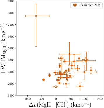
Figure 14. FWHM as a function of Mg ii–[C ii] velocity shift for quasars in our sample. Compared to Figure 10, the Mg ii line does not show a correlation with its velocity shift. Any positive correlation is driven by one outlier, CFHQS J2100–1715, whose continuum could not be fit with a power law.
Download figure:
Standard image High-resolution image
Figure 15. Luminosity at 3000 Å as a function of the C iv–Mg ii velocity shift for quasars in our sample. Our sample does not show a correlation between continuum luminosity and C iv–Mg ii blueshift.
Download figure:
Standard image High-resolution image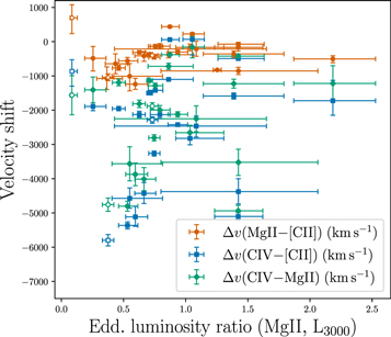
Figure 16. Velocity shifts as a function of the Eddington luminosity ratio calculated from the Mg ii line using the prescription of Vestergaard & Osmer (2009) and measured with the VW01 iron template. We tested for correlations using the Pearson correlation coefficient and found no significant correlations for Δv(CIV − [Cii]) (ρ = 0.14, p = 0.49), Δv(CIV − MgII) (ρ = −0.16, p = 0.45), and Δv(MgII − [Cii]) (ρ = 0.09, p = 0.64) with the Eddington luminosity ratio.
Download figure:
Standard image High-resolution image
Footnotes
- 13
- 14
- 15
We have used the ODR package in the scipy (Virtanen et al. 2020) Python library.
- 16