


Abstract
We perform a validation study of the latest version of the Alfvén Wave Solar atmosphere Model (AWSoM) within the Space Weather Modeling Framework. To do so, we compare the simulation results of the model with a comprehensive suite of observations for Carrington rotations representative of the solar minimum conditions extending from the solar corona to the heliosphere up to the Earth. In the low corona (r < 1.25  ), we compare with EUV images from both Solar-Terrestrial Relations Observatory-A/EUVI and Solar Dynamics Observatory/Atmospheric Imaging Assembly and to three-dimensional (3D) tomographic reconstructions of the electron temperature and density based on these same data. We also compare the model to tomographic reconstructions of the electron density from Solar and Heliospheric Observatory/Large Angle and Spectrometric Coronagraph observations (2.55 < r < 6.0
 ). In the heliosphere, we compare model predictions of solar wind speed with velocity reconstructions from InterPlanetary Scintillation observations. For comparison with observations near the Earth, we use OMNI data. Our results show that the improved AWSoM model performs well in quantitative agreement with the observations between the inner corona and 1 au. The model now reproduces the fast solar wind speed in the polar regions. Near the Earth, our model shows good agreement with observations of solar wind velocity, proton temperature, and density. AWSoM offers an extensive application to study the solar corona and larger heliosphere in concert with current and future solar missions as well as being well suited for space weather predictions.
Export citation and abstract BibTeX RIS
1. Introduction
Predicting space weather events and their geomagnetic effects requires accurate physics-based modeling of the solar atmosphere, extending from the upper chromosphere, into the corona and including the heliosphere. In the last few decades, extensive resources have been used to develop both analytic and numerical modeling techniques (Mikić et al. 1999; Groth et al. 2000; Roussev et al. 2003; Cohen et al. 2007; Feng et al. 2011; Evans et al. 2012). In addition, a wealth of observational data are now available (Air Force Data Assimilation Photospheric flux Transport—Global Oscillation Network Group (ADAPT–GONG), Arge et al. 2010; Solar Dynamics Observatory (SDO)/Atmospheric Imaging Assembly (AIA), Lemen et al. 2012; Solar-Terrestrial Relations Observatory (STEREO), Howard et al. 2008; Solar and Heliospheric Observatory (SOHO)/Large Angle and Spectrometric COronagraph (LASCO), Brueckner et al. 1995; InterPlanetary Scintillation (IPS), Jackson et al. 1998) to both drive and validate these models. The state-of-the-art three-dimensional (3D) extended MHD models that have been developed, improved and validated with observations over time provide a comprehensive understanding of the coronal structure, heating, and solar wind acceleration in the context of a fluid description.
Modern global models incorporate Alfvén wave turbulence, a physical mechanism for which the measurements of the Mariner 2, 4, 5 spacecraft established firm evidence of occurrence in the solar wind and the heliosphere (Coleman 1968; Belcher & Davis 1971). Based on this discovery, one-dimensional (1D) models incorporating Alfvén waves were developed (Alazraki & Couturier 1971; Belcher & Davis 1971), followed by two-dimensional models for the solar corona (Bravo & Stewart 1997; Ruderman et al. 1998; Usmanov et al. 2000). The interaction between forward-propagation and reflected Alfvén waves, leading to a nonlinear turbulent cascade and hence coronal heating, was first discussed in models described by Velli et al. (1989), Zank et al. (1996), Matthaeus et al. (1999), Suzuki & Inutsuka (2006), Verdini & Velli (2007), Cranmer (2010), Chandran et al. (2011), and Matsumoto & Suzuki (2012). Recently, 3D models simulating the solar corona have been developed (Lionello et al. 2009; Downs et al. 2010; van der Holst et al. 2010).
Another aspect vital to coronal modeling is energy partitioning among particle species. It is now known that the electron and ion temperatures are quite different beyond 2  , as the plasma becomes collisionless (Hartle & Sturrock 1968). The simplest description is a single fluid approach with separate temperatures for electrons and protons, which was developed by Tu & Marsch (1995), Laitinen et al. (2003), and Vainio et al. (2003) by including Alfvén waves accounting for the heating and acceleration of the solar wind plasma. Using remote observations from Ultraviolet Coronagraph Spectrometer, Kohl et al. (1998) and Li et al. (1998) showed the proton temperature anisotropy in the coronal holes. The perpendicular (to the local magnetic field direction) ion temperature was found to be much larger than the parallel ion temperature in the solar corona as well as the inner heliosphere, as seen in Helios observations (Marsch et al. 1982). This temperature anisotropy appeared in various 1D numerical models, e.g., Leer & Axford (1972) and Chandran et al. (2011) as well as in 2D models, e.g., Vásquez et al. (2003) and Li et al. (2004).
Our coronal and solar wind model, the Alfvén Wave Solar atmosphere Model (AWSoM) is a component within the Space Weather Modeling framework (SWMF; Tóth et al. 2012) and follows similar lines of development to provide a self-consistent physics-based global description of coronal heating and solar wind acceleration (Sokolov et al. 2013; van der Holst et al. 2014). AWSoM inherits many aspects of the model of van der Holst et al. (2010), including a description of low-frequency forward- and counter-propagating Alfvén waves that nonlinearly interact resulting in a turbulent cascade and dissipative heating. In addition, there are separate temperatures for electrons and protons with collisional heat conduction applied only to electrons and radiative losses based on the Chianti model (Dere et al. 1997). AWSoM is significantly advanced by extending the model to the base of the transition region and balanced turbulence (Sokolov et al. 2013). Later model advances (van der Holst et al. 2014; Meng et al. 2015) include a self-consistent treatment of Alfvén wave reflection and a stochastic heating model by Chandran et al. (2011) as well as a description of proton parallel and perpendicular temperatures and kinetic instabilities based on temperature anisotropy and plasma beta.
AWSoM is a data-driven model capable of simulating the detailed 3D structure of the corona with boundary conditions supplied by GONG or Helioseismic and Magnetic Imager (HMI) synoptic magnetic maps. These data, combined with the physical processes of wave dissipation, heat conduction, and radiative cooling, give AWSoM the capability of capturing the temperature and mass density structure of the corona. As a result, synthetic EUV images can be made with AWSoM, which reproduce multiwavelength observations including features such as coronal hole morphology and active region brightness (Sokolov et al. 2013; van der Holst et al. 2014), similar to those first produced by Downs et al. (2010). The model results have been compared to in situ observations from ACE, Wind, and STEREO data at 1 au (Meng et al. 2015; van der Holst et al. 2019) and to observations from Ulysses (Oran et al. 2013; Jian et al. 2016). In addition to steady-state conditions, our solar wind models have been applied to study coronal mass ejections (CMEs). Manchester et al. (2012) and Jin et al. (2013) applied the model of van der Holst et al. (2010) to show that the two-temperature model accurately reproduced the CME shock structure without unphysical heat precursors ahead of CMEs, which can appear due to electron heat conduction applied to ions. Manchester et al. (2014) and Jin et al. (2017) also simulated observed fast CME events with the Gibson-Low (GL) flux rope model (Gibson & Low 1998) and demonstrate the ability to reproduce many observed features near the Sun and at 1 au by comparing with observations from SDO, SOHO, and STEREO A/B.
In this paper, we follow the work of Jin et al. (2012) and perform a comprehensive validation of the coronal model. We describe the solar corona–inner heliosphere simulation results for solar minimum conditions using the latest version of the AWSoM model within the SWMF. The input is obtained from ADAPT–GONG global magnetic maps for Carrington rotations, CR 2208 (2018 September 02 to 2018 September 29) and CR 2209 (2018 September 29 to 2018 October 26). We compare the model predicted results with an extensive suite of observations ranging from near the Sun up to 1 au. The observations include STEREO-A EUVI and AIA images, tomographic reconstructions of electron density and temperatures from AIA data between 1.025 and 1.225  and reconstruction of the electron density from LASCO-C2 data between 2.55 to 6
  . We also include model comparisons with IPS data at 20
  , 100
, 100  , and 1 au. Finally, comparisons with OMNI data at 1 au are shown. The paper is organized as follows, Section 2 details the AWSoM model characteristics, input global photospheric magnetic field maps, and simulation parameters. In Section 3, we validate the results of the solar wind model for CR 2208 and CR 2209 with observations. We conclude with a summary and discussion in Section 4.
2. Computational Model and Simulation
2.1. Alfvén Wave Solar Atmosphere Model (AWSoM) Description
We describe here the main characteristics of the 3D global MHD AWSoM model included within the Space Weather Modeling Framework (Tóth et al. 2012). This model uses the numerical Block-Adaptive-Tree-Solarwind-Roe-Upwind-Scheme (BATS-R-US; Powell et al. 1999) to solve the MHD equations. AWSoM extends from the upper chromosphere, through the transition region, into the solar corona and the inner heliosphere (up to 1 au and beyond).
AWSoM includes isotropic electron temperature as well as anisotropic (distinct perpendicular and parallel) proton temperatures. It addresses the coronal heating and solar wind acceleration with low-frequency Alfvén wave turbulence. The wave pressure gradient accelerates the plasma and wave dissipation heats it. The model includes nonlinear interaction between outward-propagating and counter-propagating (reflected) Alfvén waves that gives rise to a transverse turbulent cascade from the outer scale to smaller perpendicular scales where dissipation and coronal heating takes place. To distribute the coronal heating among three temperatures, AWSoM uses the physics-based theories of linear wave damping and stochastic heating. At the proton gyro-radius scale the kinetic Alfvén wave turbulence has a range of parallel wave numbers, but for the damping rates we need to assign a single wave number. This wave number is determined by the critical balance condition in which we set the Alfvén wave frequency equal to the inverse of the cascade time of the minor wave (Lithwick et al. 2007). This is an improvement with respect to the energy partitioning used in Chandran et al. (2011) and van der Holst et al. (2014), where the cascade time of the major wave was used. This change leads to more electron heating and less solar wind acceleration, resulting in significantly improved model-data comparisons. Details of the changes in the energy partitioning will be reported in B. van der Holst et al. (2020, in preparation). No ad hoc heating functions are used. The model also includes the electron heat conduction both for the collisonal and collisonless regimes. MHD equations included in the AWSoM model are described in detail in van der Holst et al. (2014).
2.2. Input Global Magnetic Maps
The primary data input to solar MHD models is the synoptic magnetogram which provides estimates of the photospheric magnetic field of the Sun. These synoptic maps are essential for modeling the solar corona and the solar wind accurately for the purpose of prediction. Therefore, it is important that the magnetic field estimates of the Sun are reliable. GONG provides such standard synoptic magnetograms. These are full disk surface maps of the radial component of the photospheric magnetic field. To create a synoptic map, first the full disk line-of-sight images are merged and mapped to heliographic coordinates. It is assumed that the photospheric magnetic field is radial and that the Sun rotates as a solid body with a 27.27 day rotation rate. The remapped images are then merged together for a Carrington rotation with parts of the overlapping coordinates merged. In addition, as the polar fields are not well observed from the ecliptic, the processing in GONG maps estimates them by polynomial fits to the observed fields from neighboring latitudes leading to uncertainties. These uncertainties in the polar magnetic flux distribution propagate into the solar wind simulations in the coronal models (Bertello et al. 2014).
Worden & Harvey (2000) developed a model to create synchronic synoptic maps which evolve the magnetic flux on the Sun based on super-granulation, diffusion, differential rotation, meridional circulation, flux-emergence, and data merging. These processes are used in the model to provide missing data where observations are not available. The Air Force Data Assimilation Photospheric Flux Transport (ADAPT; Arge et al. 2010, 2013; Henney et al. 2012) model incorporates this Worden & Harvey (2000) model and the Los Alamos National Lab data assimilation code (Hickmann et al. 2015) to create synchronic maps based on observations and dynamic physical processes. The data assimilation technique produces multiple realizations of the magnetic field maps to account for different parameters and their uncertainties in the photospheric flux-transport model. ADAPT maps using observations from different instruments are available at https://www.nso.edu/data/nisp-data/adapt-maps/.
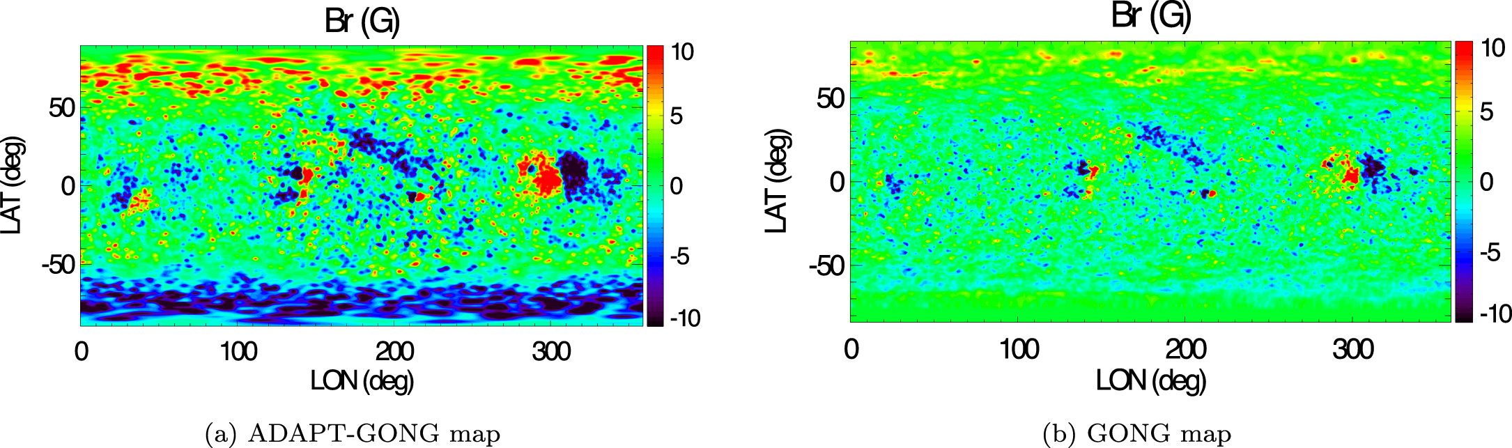
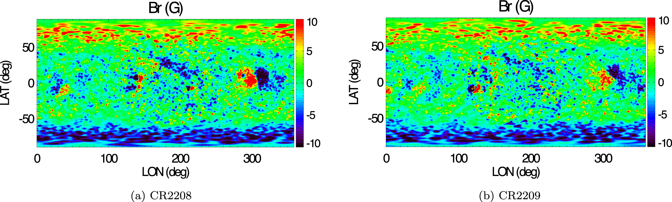
Figure 1 shows the ADAPT–GONG and GONG global maps for CR 2208. The two maps show significant differences, especially in the polar regions. We find that using ADAPT–GONG maps as input to the AWSoM model produces significantly better results in comparison to using GONG maps. Therefore, in this work we use ADAPT–GONG global magnetic maps for both CR 2208 and CR 2209. These are shown in Figure 2.
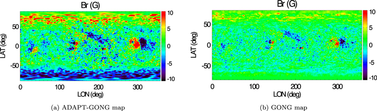
Figure 1. Radial magnetic fields for CR 2208 using one realization of the ADAPT–GONG ensemble of synchronic maps (left) and the GONG synoptic map (right) provided by the National Solar Observatory (NSO). The magnetic fields in this plot are saturated at ±10 G.
Download figure:
Standard image High-resolution image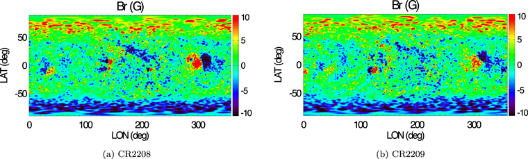
Figure 2. Input radial magnetic field maps for CR 2208 (left) and CR 2209 (right) using ADAPT–GONG global maps. The magnetic fields in this plot are saturated at ±10 G.
Download figure:
Standard image High-resolution image2.3. Simulation Parameters and Setup
In this section, we set up the solar wind model. The SWMF facilitates the simultaneous execution and coupling of different components of the space environment covering various physics models. Besides space weather applications for the Sun–Earth system, the SWMF has been used for many planetary, comet, and moon applications (Tóth et al. 2005). Tools for SWMF and numerical schemes of the BATS-R-US MHD solver are described in Tóth et al. (2012). We use the solar corona and inner heliosphere components of SWMF in this paper. The solar corona model uses a 3D spherical grid and the inner heliosphere model uses a Cartesian grid, with an overlapping buffer grid which couples the solutions from solar corona over to inner heliosphere. The computational domain for the solar corona model lies within the radial coordinate ranging from 1  to 24
to 24  using a radially stretched grid and the z-axis aligned with the rotation axis. The stretched grid, with a radial resolution of 0.001
  close to the Sun provides a high numerical resolution for the steep density gradients in the upper transition region. The Adaptive Mesh Refinement for solar corona, between 1.0
  and 1.7
  refines the angular cell size to
  . Outside this radial range, the grid is one level coarser, with an angular resolution of 2.8°. The MHD equations described in van der Holst et al. (2014) are solved in the heliographic rotating frame including contributions from the Coriolis and centrifugal forces. The heliospheric current sheet (HCS) is resolved with two extra levels of refinement with 1.4° cell size in the longitude and latitude directions. We decompose the solar corona domain into 6 × 8 × 8 grid blocks. The number of cells used in the solar corona component is of the order of 3 million and local time stepping is used for speeding up the convergence of the simulation to a steady-state solar wind solution.
The initial as well as the boundary condition for the magnetic field is specified by the synchronic ADAPT–GONG maps provided by NSO. We use a Potential Field Source Surface Model (PFSSM) to extrapolate the 3D magnetic field (from the 2D photospheric magnetic field maps), which we represent as spherical harmonics. The source surface is taken to be at r = 2.5  . Beyond the source surface the magnetic field is purely radial. The initial condition is specified by all the components of the magnetic field while the radial component of the magnetic field specifies the boundary condition. At the inner boundary, the radial component of the magnetic field is held fixed (according to the PFSSM solution) and the latitudinal and longitudinal components of the magnetic field are allowed to adjust freely in response to the interior dynamics.
The inner boundary of the model is at the base of the transition region (≈1.0  ) which is artificially broadened to obtain higher resolution near the Sun (Lionello et al. 2009; Sokolov et al. 2013). The density at the inner boundary is taken to be an overestimate, Ne = Ni = N⊙ = 2 × 10¹⁷ m−3 corresponding to the isotropized temperature values, Te = Ti = Ti∥ = T⊙ = 50,000 K. This ensures that the base is not affected by chromospheric evaporation and the upper chromosphere extends for the density to fall rapidly to correct (lower) values (Lionello et al. 2009). To account for the energy partitioning between electrons and protons, the stochastic heating exponent and amplitude are set to 0.21 and 0.18 respectively (Chandran et al. 2011). The Poynting flux of the outgoing wave sets the empirical boundary condition for the Alfvén wave energy density (w). As SA ∝ VA w ∝ B⊙, the proportionality constant is estimated as
  Wm−2T−1, where SA is the Poynting flux, VA is the Alfvén wave velocity, and B⊙ is the field strength at the inner boundary (Sokolov et al. 2013). The correlation length (L
 ) of the Alfvén waves (transverse to the magnetic field direction) is proportional to B−1/2. The proportionality constant,
  is an adjustable input parameter in the model and is set to 1.5 × 10⁵ m
  . To synthesize high-resolution line-of-sight (LOS) EUV images from the model, we use the fifth-order numerical scheme with MP5 limiter (Suresh & Huynh 1997; Chen et al. 2016) within 1.5
  , and the standard second-order shock-capturing schemes in the remainder of the solar corona region (Tóth et al. 2012).
The computational domain for the inner heliosphere component is a cube surrounding the spherical domain of solar corona extending −250  ≤ (x, y, z) ≤ 250
  . The adaptive Cartesian grid ranges from a cell size less than 0.5
  to ≈8
to ≈8  . The total number of cells for the inner heliosphere component is of the order of 8 million.
The solar corona component runs for 60,000 steps to reach a steady state. The solar corona and inner heliosphere components are then coupled once. Following which, solar corona is switched off and inner heliosphere runs for 5000 steps until it converges. In this paper, we show simulation results for Carrington rotations CR 2208 and CR 2209. The two Carrington rotations represent the near solar minimum conditions during the end of the decaying phase of solar cycle 24, close to the beginning of solar cycle 25. The ADAPT–GONG global magnetic maps used as input for these rotations are shown in Figure 2. The following section describes the results of the solar corona–inner heliosphere simulations when compared with an extensive set of observations ranging from the lower corona up to 1 au.
3. Comparisons with Observations
In this section, we present the results of steady-state solar wind simulations for both CR 2208 and CR 2209 representing solar minimum conditions. The results shown here use one of the 12 realizations of the ADAPT–GONG maps. We compare the steady-state AWSoM model simulations with observations at various radial distance ranges. Beginning from close to the Sun (Extreme Ultraviolet images, STEREO-A/EUVI and SDO/AIA), followed by tomographic reconstructions of plasma parameters using AIA data, SOHO/LASCO-C2 data, and IPS data. Finally, we compare the model results with 1 au observations (OMNI data).
3.1. Extreme UltraViolet Images (EUVI)
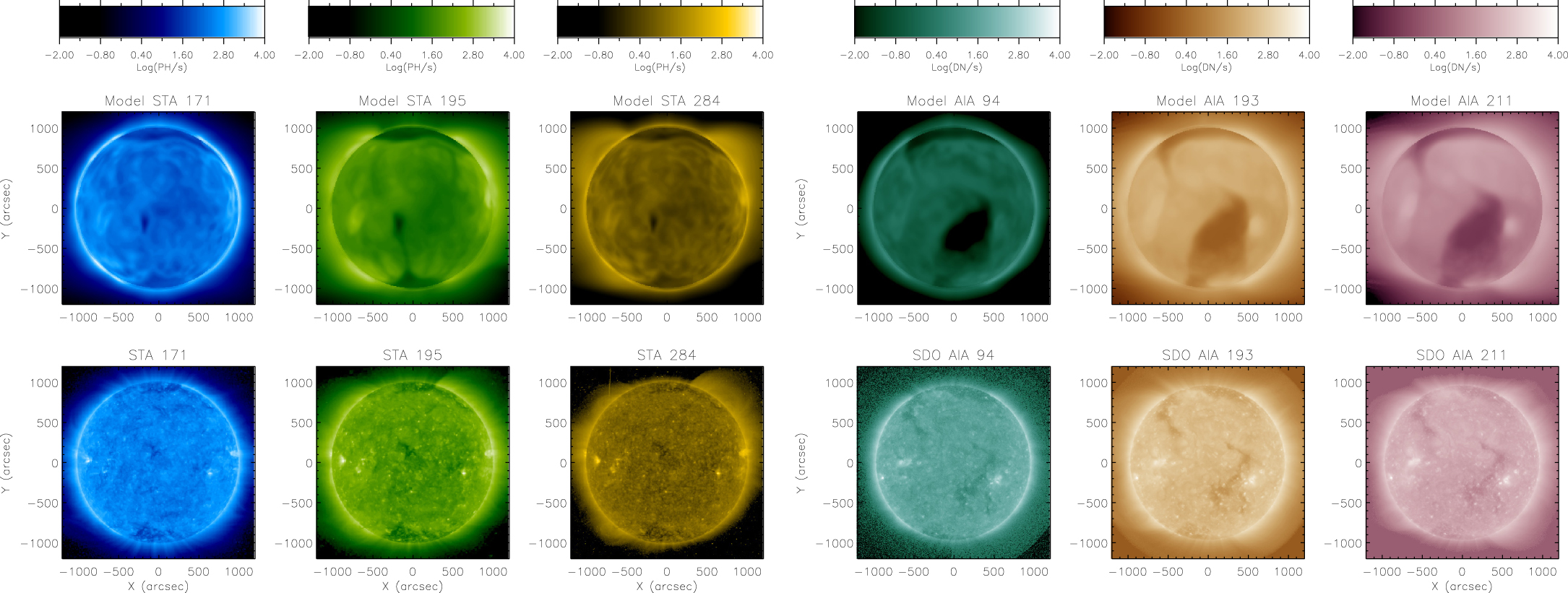
The model simulated electron density and temperature are used to synthesize extreme ultraviolet (EUV) line-of-sight (LOS) images. These are compared to the multiwavelength EUV observations from STEREO-A/EUVI and SDO/AIA. Figures 3 and 4 show these comparisons for CR 2208 and CR 2209 respectively. Synthetic images are shown corresponding to STEREO-A/EUVI, 171 Å, 195 Å, and 284 Å bands and SDO/AIA, 94 Å, 193 Å, and 211 Å bands, corresponding to Fe emission lines. The observation time for CR 2208 is ≈22: 00: 00 UT on 2018 September 15 and for CR 2209 it is ≈06: 00: 00 UT on 2018 October 13. These times coincide with the central meridian times of the ADAPT–GONG map used for the respective simulations. No STEREO-B images are available for comparison, as the spacecraft ceased to operate before these rotations.
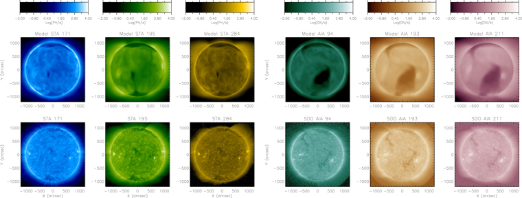
Figure 3. Comparison of model synthesized LOS EUV images with STEREO-A/EUVI (left) for 171, 195, and 284 Å and SDO/AIA extreme ultraviolet images (right) for 94, 193, and 211 Å for CR 2208. The top panels show the LOS images from the AWSoM model and the bottom panels show the observations.
Download figure:
Standard image High-resolution imageFor each rotation, the top row shows the model simulated LOS EUV image while the bottom row shows the observation. The corresponding wavelengths are indicated at the top of each panel. As mentioned before, this model accounts for the partial reflection of outward-propagating waves and their interaction with the counter-propagating (reflected) waves. This leads to turbulent cascade dissipation and hence, coronal heating. As a result, in regions of strong magnetic fields, such as, active regions, stronger reflection and therefore more dissipation occurs, which results in an intensified EUV emission.
The LOS images are produced under the assumption that for all wavelengths considered here, the plasma is optically thin. In general, there tends to be a dominant stray light component in EUV images caused by long-range scatter. Shearer et al. (2012) showed that 70% of the emission in coronal holes on the solar disk is made up of this stray light in EUVI. The STEREO-A/EUVI observations shown in Figures 3 and 4 are stray-light corrected. We see the extended coronal hole in the north reproduced in the model results. The narrow southern coronal hole is also visible in the model simulations in all wavelengths in the STEREO-A/EUVI images. The average brightness of the EUV images is captured quantitatively by the model simulations for both STEREO-A/EUVI and SDO/AIA images. However, our model results show coronal holes that are darker in comparison to the AIA observations, which is at least partially due to the neglected scattering in the synthetic EUV images.

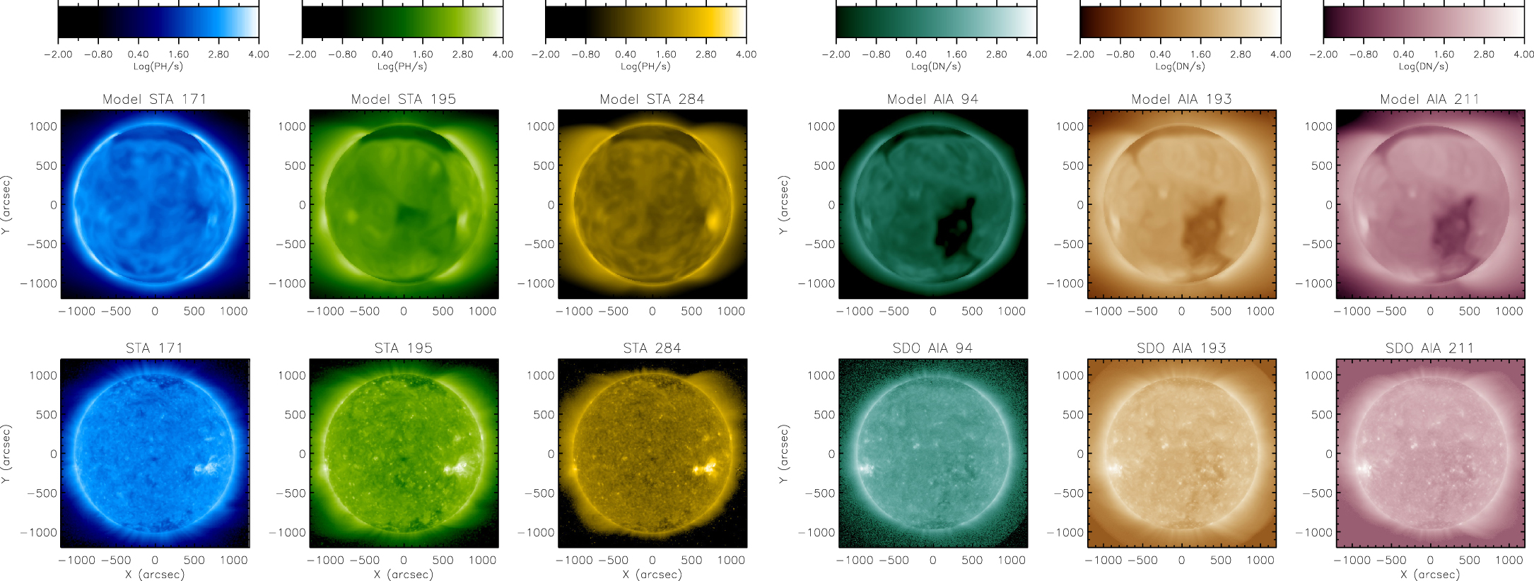
Figure 4. Comparison of model synthesized LOS EUV images with STEREO-A/EUVI (left) for 171, 195, and 284 Å and SDO/AIA extreme ultraviolet images (right) for 94, 193, and 211 Å for CR 2209. The top panels show the LOS images from the AWSoM model and the bottom panels show the observations.
Download figure:
Standard image High-resolution imageWith the exception that our model shows far less brightness in coronal holes, especially in comparison to AIA observations, we find that the coronal hole locations are pretty well captured in our analyses. As expected, the small-scale structure is partially captured, with larger active regions clearly reproduced. We note that the steady-state simulation is performed for a synchronic magnetic field map over a complete Carrington rotation whereas the observations are for particular time stamps, thus, the model cannot reproduce time-dependent activity during the rotation.
3.2. Differential Emission Measure Tomography (DEMT)
DEMT is a solar rotational tomography (SRT) technique which employs a time series of EUV images to reconstruct the 3D Differential Emission Measure (DEM) in the solar corona (Frazin & Kamalabadi 2005; Frazin et al. 2009; Vásquez 2016). DEMT combines the EUV tomography in several pass bands with local DEM analysis to produce 3D distributions of the coronal electron density and temperature in the radial range of 1.025–1.225  . Vásquez et al. (2010) and Lloveras et al. (2017) used DEMT for a comparative analysis of the coronal structure during solar minima.
In this study, the DEMT analysis for CR 2208 and CR 2209 uses the superior high-cadence SDO/AIA data to have better signal-to-noise ratio. In this work, the technique uses for the first time a newly implemented 3D regularization scheme instead of the latitude–longitude regularization scheme used in the previous DEMT efforts. This implies that the tomography results are now more trustworthy at the lowest heights and boundary-induced artifacts are minimized. For each instrument, the DEMT analysis entails a cross-validation study to determine the optimal regularization level. This level is different for each wavelength band and is sensitive to the activity level of the Sun. We obtained tomographic reconstructions for each of the rotations using 1/2 rotation of off-limb data, fully blocking the disk (hollow tomography). Here, we show comparisons with the hollow tomography reconstructions for both CR 2208 and CR 2209.
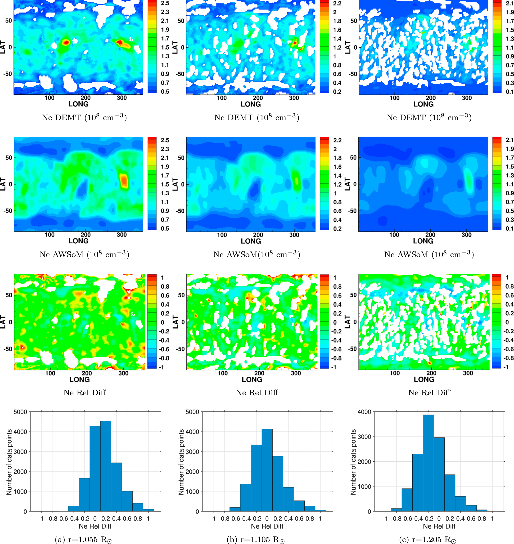
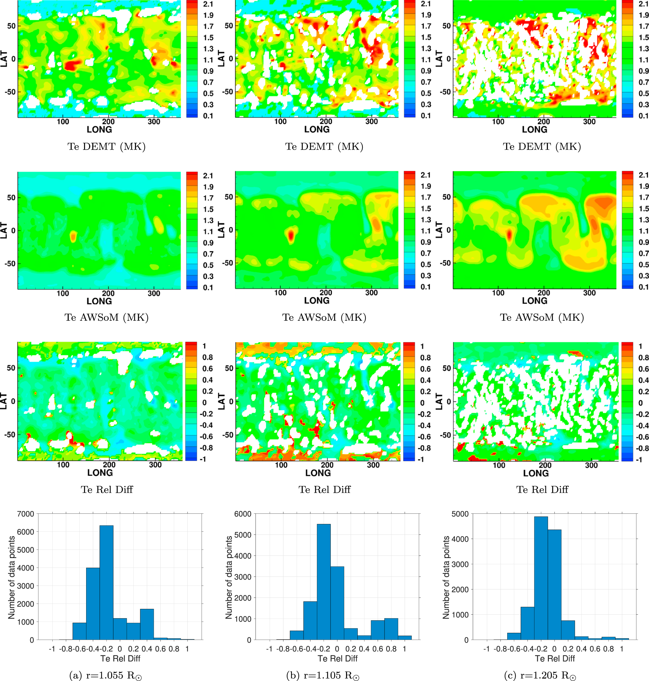
Figures 5 and 6 show the comparisons between the DEMT reconstructed electron density and temperature and the model output, respectively, at three radial distances, r = 1.055, 1.105, and 1.205  . The top two panels in Figure 5 show the longitude–latitude maps for the tomographic electron density (Ne DEMT) and model output (Ne AWSoM) in units of 108 cm−3. The white regions in the DEMT maps are zones not reliably reconstructed by the tomography, as discussed below. The bottom two panels show the relative difference in electron density, Ne Rel Diff
  and the corresponding histogram distribution. Figure 6 shows the same results for the electron temperature in units of MK. Top two panels show Te DEMT and Te AWSoM, and the bottom two panels show Te Rel Diff
  . Figures 7 and 8 show the same quantities for CR 2209.

Figure 5. Comparison of tomographic reconstructions of electron density from EUV observations and AWSoM model simulation results for CR 2208 at (a) 1.055  , (b) 1.105
  , and (c) 1.205
  . First and second rows show the 3D reconstructed density from SDO/AIA observations using DEMT (Ne DEMT) and the model predicted density (Ne AWSoM), respectively, in units of 108 cm−3. The third row depicts the relative difference between the observations and model results. The quantity shown is Ne Rel Diff =
  . Bottom row shows the histogram distribution for Ne Rel Diff.
Download figure:
Standard image High-resolution image
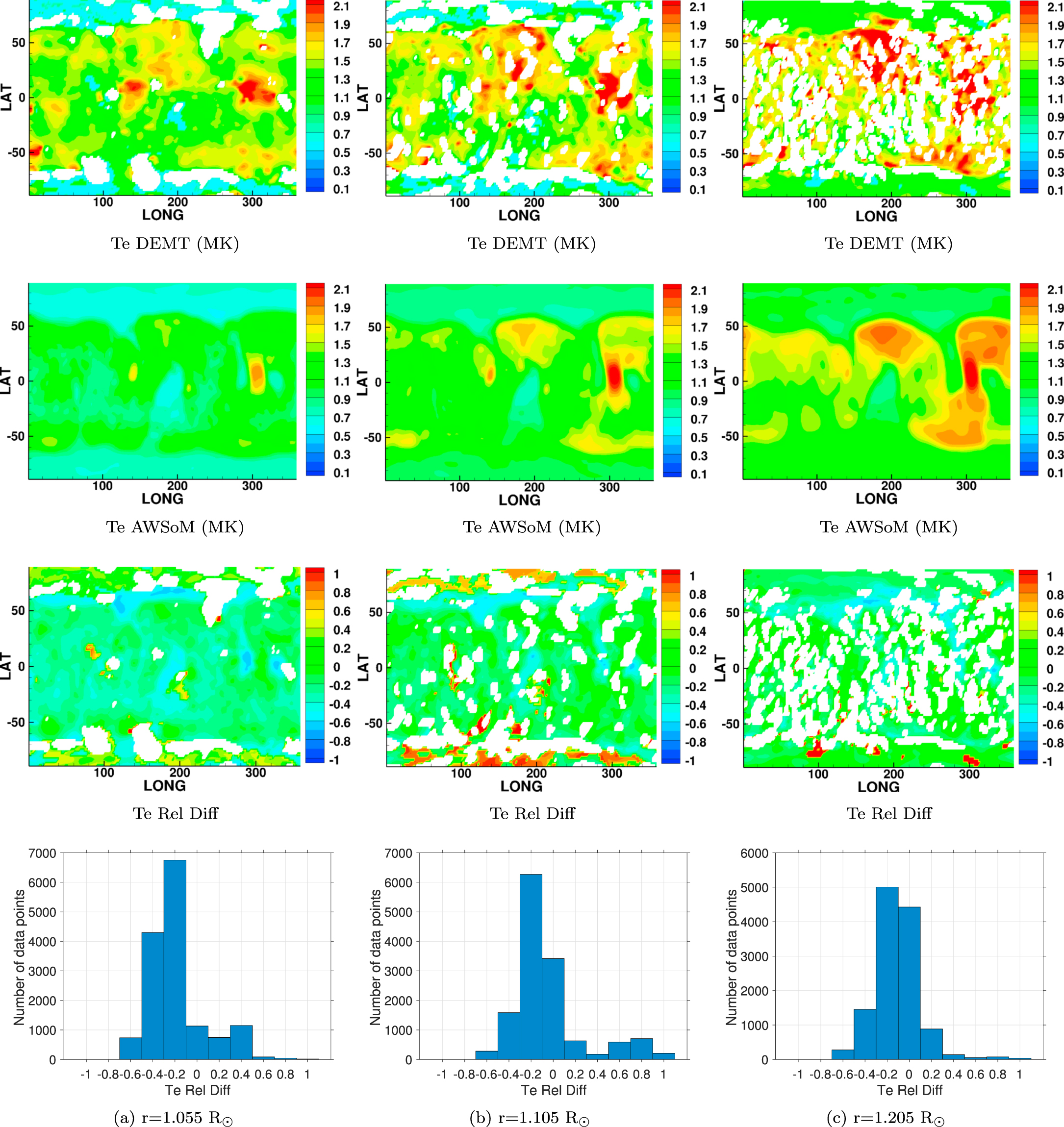
Figure 6. Comparison of tomographic reconstructions of electron temperature from EUV observations and AWSoM model simulation results for CR 2208 at (a) 1.055  , (b) 1.105
  , and (c) 1.205
  . First and second rows show the 3D reconstructed temperature from SDO/AIA observations using DEMT (Te DEMT) and the model predicted temperature (Te AWSoM), respectively, in units of 106 K (MK). The third row depicts the relative difference between the observations and model results. The quantity shown is Te Rel Diff =
  . Bottom row shows the histogram distribution for Te Rel Diff.
Download figure:
Standard image High-resolution image
Figure 7. Comparison of tomographic reconstructions of electron density from EUV observations and AWSoM model simulation results for CR 2209 at (a) 1.055  , (b) 1.105
  , and (c) 1.205
  . First and second rows show the 3D reconstructed density from SDO/AIA observations using DEMT (Ne DEMT) and the model predicted density (Ne AWSoM), respectively, in units of 108 cm−3. The third row depicts the relative difference between the observations and model results. The quantity shown is Ne Rel Diff =
  . Bottom row shows the histogram distribution for Ne Rel Diff.
Download figure:
Standard image High-resolution image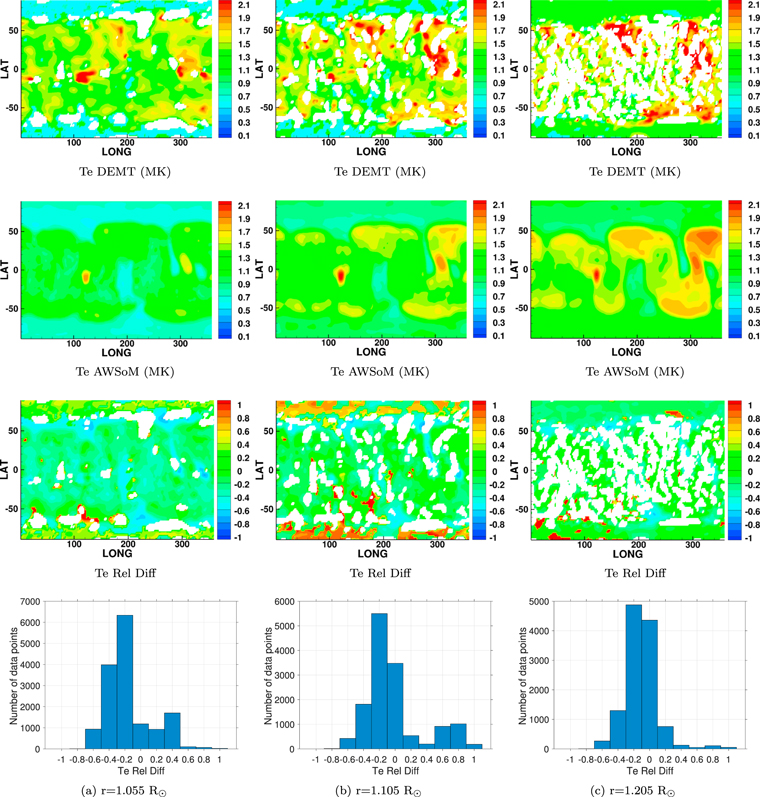
Figure 8. Comparison of tomographic reconstructions of electron temperature from EUV observations and AWSoM model simulation results for CR 2209 at (a) 1.055  , (b) 1.105
  , and (c) 1.205
  . First and second rows show the 3D reconstructed temperature from SDO/AIA observations using DEMT (Te DEMT) and the model predicted temperature (Te AWSoM), respectively, in units of 106 K (MK). The third row depicts the relative difference between the observations and model results. The quantity shown is Te Rel Diff =
  . Bottom row shows the histogram distribution for Te Rel Diff.
Download figure:
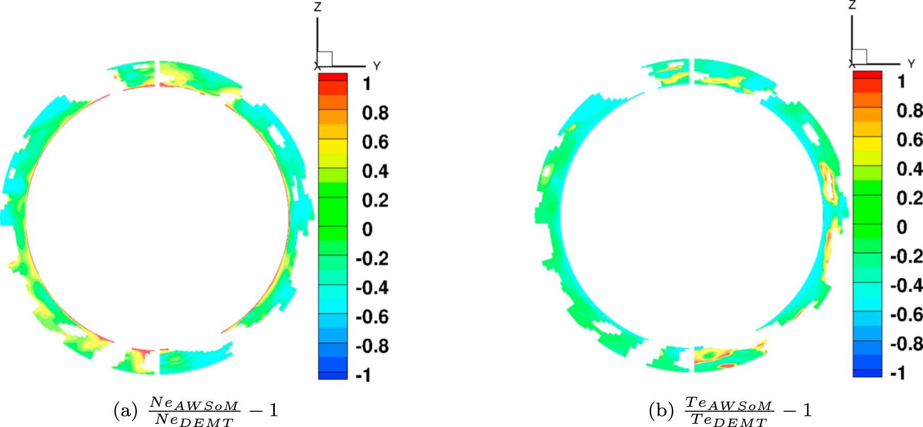
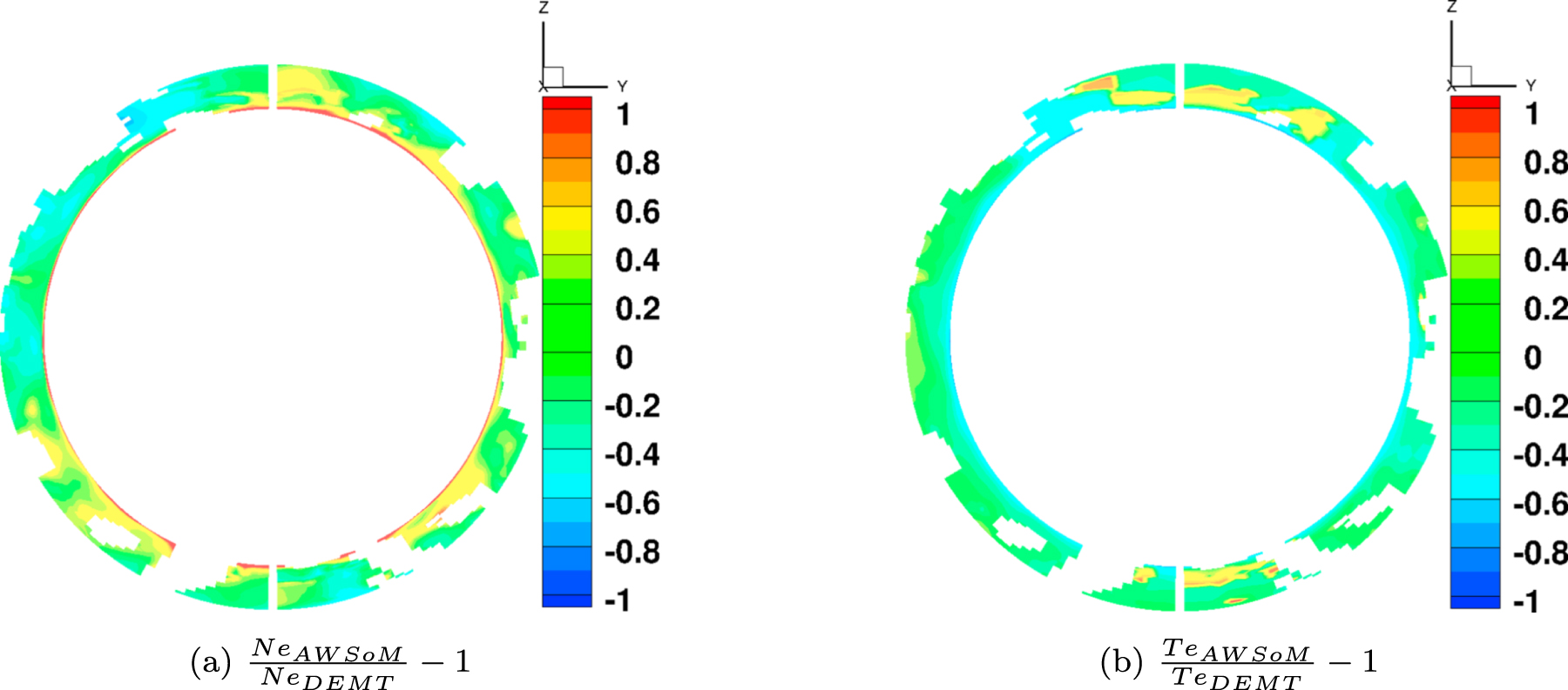
Standard image High-resolution imageThe white regions in the DEMT maps in Figures 5–10 are those for which the tomography cannot provide a reliable reconstruction. These regions include cells where the reconstructed emissivity, forced to be positive, is null in at least one of the bands. These are called zero-density-artifacts, which are caused by coronal dynamics not accounted by the DEMT technique (see, Frazin et al. 2009; Lloveras et al. 2017).

Figure 9. X = 0 slice for CR 2208 showing the relative difference in (a) electron density and (b) electron temperature for 1.025 < r < 1.225  .
.
Download figure:
Standard image High-resolution image
Figure 10. X = 0 slice for CR 2209 showing the relative difference in (a) electron density and (b) electron temperature for 1.025 < r < 1.225  .
.
Download figure:
Standard image High-resolution imageIn cells where DEMT provides positive emissivities, the local-DEM (LDEM) of each voxel is determined. The resulting DEM is then evaluated in each voxel for consistency with the tomographic reconstruction of the emissivity in all three bands. To that end, we define a quantity, R which is the fractional difference between the tomographic emissivity and the synthetic one predicted by the DEM of that voxel, averaged for three EUV bands. In other words, R is a measure of the degree of success of the LDEM in reproducing the tomographically reconstructed emissivity in all three bands. R lies between 0 and 1, where 0 means a good agreement. Regions that have R > 0.25 are excluded, which are the white regions in the data–model comparisons.
We also show the X = 0 slice for relative difference in density and temperature in Figure 9 for CR 2208 and Figure 10 for CR 2209. It can be seen that from the innermost boundary of the tomographic computational domain (r = 1.025  ) up to about 1.055
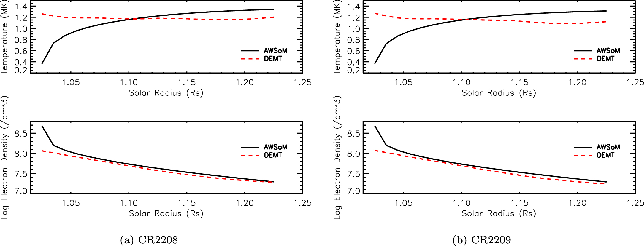
  , the model electron density is overestimated compared to the DEMT results. This overestimate is the result of artificial broadening of the transition region to be consistent with our limited numerical resolution. This is also evident from Figure 11, which shows the average (over all longitudes and latitudes) of temperature and density at different radial distances between 1.025
  and 1.225
  . The DEMT reconstructed data are shown in red and AWSoM results are shown in black for CR 2208 (left) and CR 2209 (right). We see that the model temperature converges to reconstructed values at lower heights, but the density cannot catch up. The comparisons get significantly better as we go higher radially.

Figure 11. Variation of the longitude–latitude averaged electron temperature (in MK) and log electron density (in cm−3) from AWSoM simulations (black) and DEMT reconstruction (red) for CR 2208 (left) and CR 2209 (right) with the radial distance ranging between 1.025 and 1.225 .
.
Download figure:
Standard image High-resolution imageThe steep gradients in temperature and density in the thin transition region require excessive numerical resources to resolve on a global scale. These gradients are a result of the balance of coronal heating, heat conduction, and radiative losses. Therefore, as described in Lionello et al. (2009) and Sokolov et al. (2013) the transition region is artificially broadened so as to be properly resolved with our finest grid resolution of ≈0.001  . This broadening of the transition region pushes the corona outwards. In addition, if the chromospheric density is too low, the transition region may evaporate. As described in Section 2.3, the density at the inner boundary (upper chromosphere) is taken to be an overestimate, which ensures that the base is not affected by chromospheric evaporation and the density of the upper chromosphere falls rapidly to correct (lower) values. At this level, the radiative losses are sufficiently low so that the temperature can increase monotonically with height and form the transition region. Thus, at low radial distances of about 1.025–1.055
  the AWSoM predicted density is still an overestimate compared to the DEMT reconstructed values using EUV data.
In addition, Alfvén wave heating also affects energy balance in the transition region. This heating can be improved upon, as the reflection physics through the transition region is not fully accounted for. Currently, we set an artificial upper bound for the wave reflection in the transition region based on the cascade rate (details in van der Holst et al. 2014). Hence, the coronal heating might be underestimated at the transition region which can further lower the temperature compared to the DEMT reconstructed values.
3.3. LASCO-C2 Solar Tomography
Time-dependent SRT is applied to white-light coronal images obtained with the LASCO-C2 coronagraph to produce the three-dimensional electron density distributions (Frazin et al. 2010; Vibert et al. 2016). We compare these tomographic reconstructions to the model simulated densities at heights between 2.55 and 6  . The LASCO-C2 images use most up-to-date superior instrumental corrections and calibration (Gardés et al. 2013; Lamy et al. 2017) as provided by the Laboratoire d'Astrophysique de Marseille (LAM).
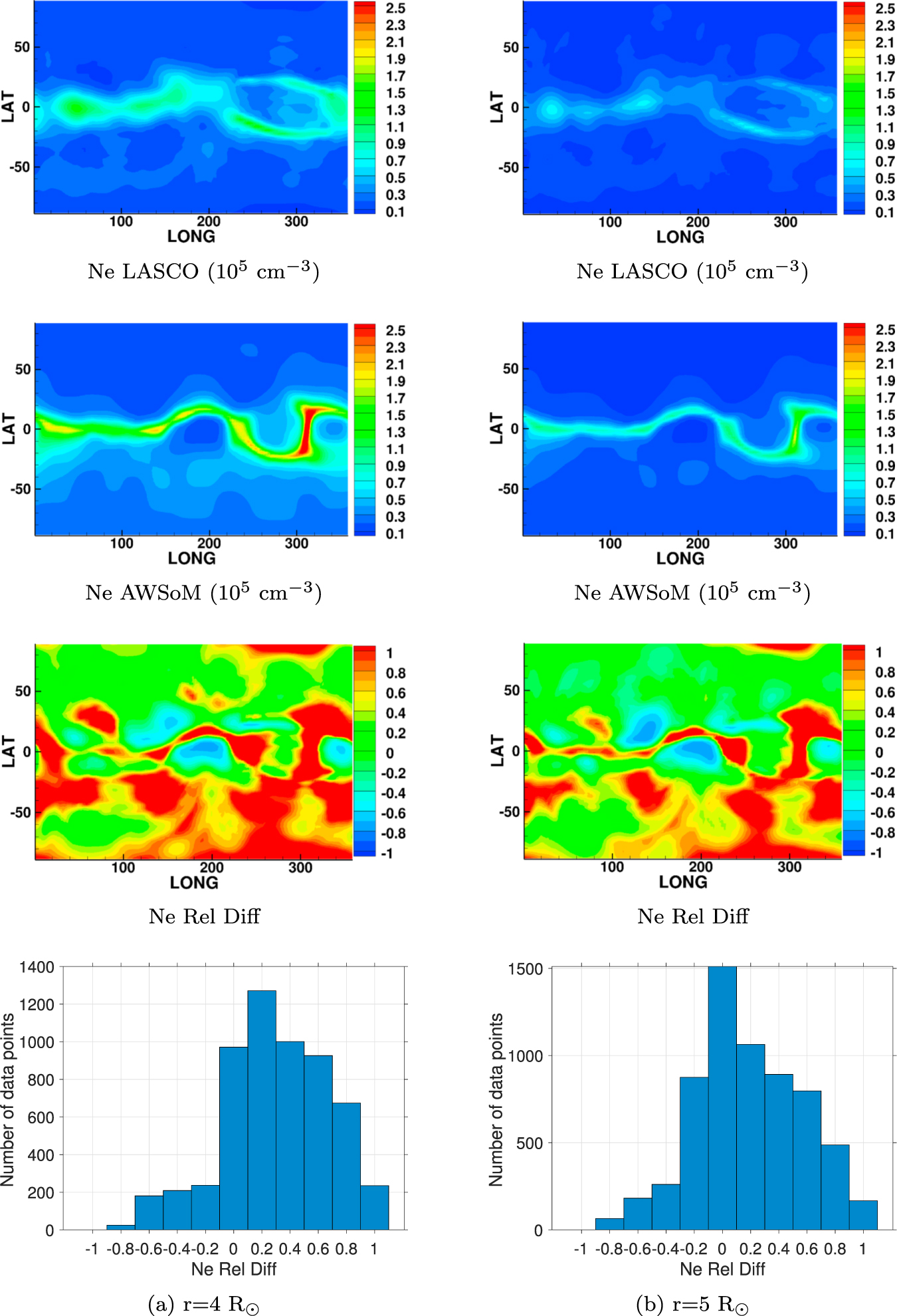
Figures 12 and 13 show the relative difference between the reconstructed coronal density and model results for CR 2208 and CR 2209 respectively. In each figure, the first two rows show the density obtained from tomography (Ne LASCO) and the density from AWSoM model results (Ne AWSoM), respectively, in units of 105 cm−3. Bottom two rows show the comparisons between tomography data and model solutions at (a) 4  and (b) 5
  and the corresponding histograms. The quantity shown here for comparison is the density difference relative to the observed tomographic density, Ne Rel Diff
  . We find that the predicted densities in the range of heliocentric heights within the LASCO FOV lie within ±20%–30% of the observed densities reconstructed from LASCO-C2. The larger discrepancy along the streamer cusp can be attributed to the underresolved features in the LASCO reconstructions. AWSoM results show a highly resolved thin current sheet with high density regions, compared to the features in LASCO that seem to be smeared out along the current sheet. Therefore, a cell-by-cell comparison shows differences that are way off in this region.

Figure 12. Comparison of LASCO-C2 reconstructed electron density and AWSoM model simulations for CR 2208 at (a) 4  and (b) 5
  . First and second rows show the LASCO 3D reconstructed density and the density predicted by the model, respectively, in units of 105 cm−3. Bottom two rows depict the quantity, Ne Rel Diff =
  , which is the relative difference between the model density and observations in the form of a latitude–longitude plot and a histogram distribution.
Download figure:
Standard image High-resolution image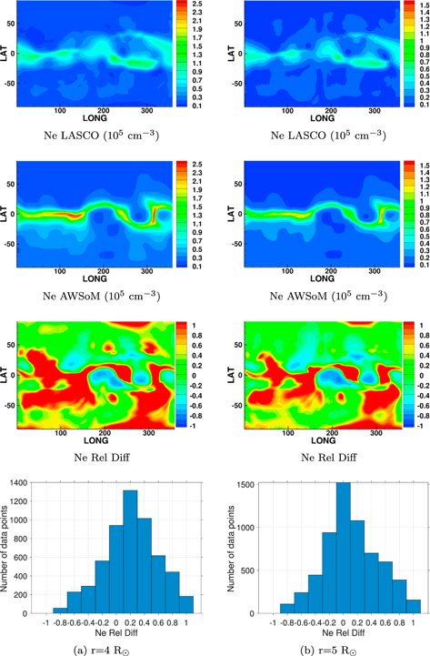
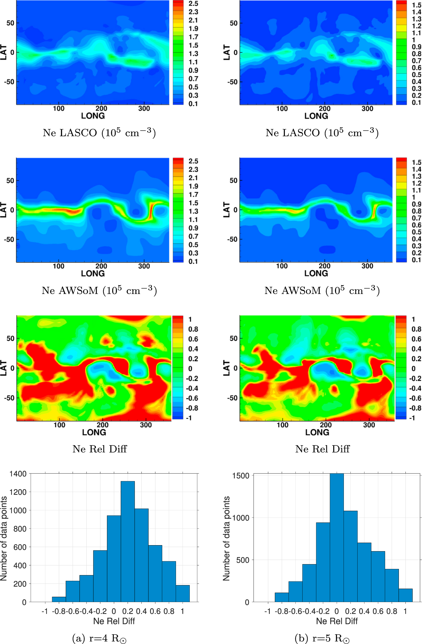
Figure 13. Comparison of LASCO-C2 reconstructed electron density and AWSoM model simulations for CR 2209 at (a) 4  and (b) 5
  . First and second rows show the LASCO 3D reconstructed density and the density predicted by the model, respectively, in units of 105 cm−3. Bottom two rows depict the quantity, Ne Rel Diff =
 , which is the relative difference between the model density and observations in the form of a latitude–longitude plot and a histogram distribution.
Download figure:
Standard image High-resolution imageWe find that that the AWSoM model produces an asymmetric density distribution between the two hemispheres, which is a direct consequence of the different sizes of the northern and southern coronal holes as seen in the EUV images. The polar asymmetry originates in the magnetic field maps for the two Carrington rotations, where the unipolar magnetic fields of the northern polar regions extend to lower latitudes compared to the southern pole. As a result, a more narrow coronal hole forms in the south for which the magnetic field has larger expansion, which in turn leads to a comparatively slower and denser solar wind. This can explain the over dense regions in the southern hemisphere of the AWSoM model results in the LASCO FOV compared to the LASCO reconstructions. This asymmetry in density (and speed) is also seen further out in the inner heliosphere (Section 3.4).
3.4. InterPlanetary Scintillation
We use the IPS time-dependent, kinematic 3D reconstruction technique to obtain the solar wind parameters in the inner heliosphere. Time-dependent results can be extracted at any radial distance within the reconstructed volume. Here, we show the IPS data and AWSoM model comparisons at r = 20  , 100
, 100  , and 1 au. The University of California, San Diego (UCSD), has developed an iterative Computer Assisted Tomography program (Jackson et al. 1998, 2003, 2010, 2011, 2013, Hick & Jackson 2004, Yu et al. 2015) that incorporates remote sensing data from Earth to a kinematic solar wind model to provide 3D reconstructed velocity distributions over the inner heliosphere.
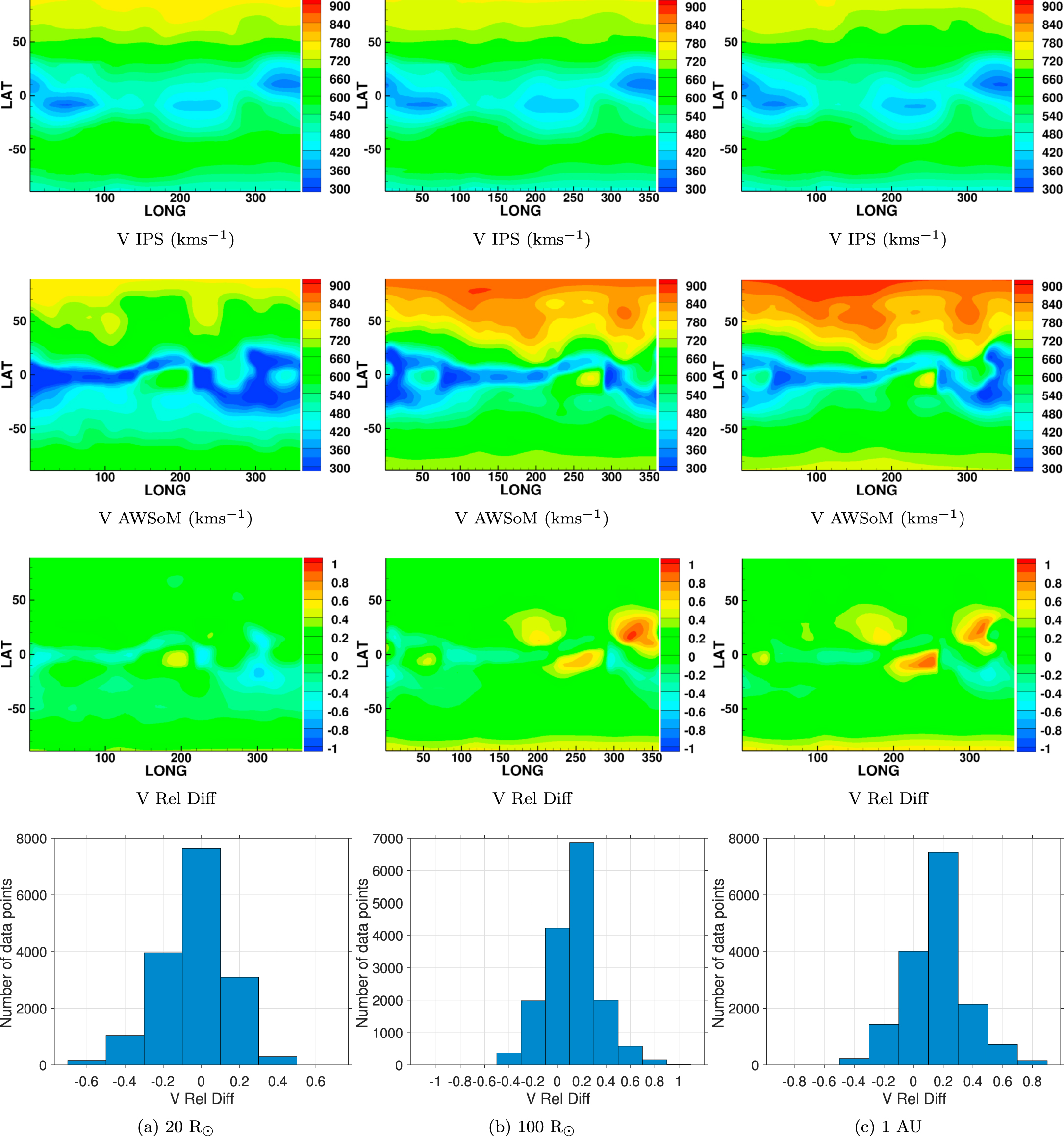
Figures 14 and 15 show the velocity comparisons of AWSoM model results for CR 2208 and CR 2209, respectively, with the IPS reconstructions at three radial distances, 20  , 100
, 100  , and 1 au. At each distance, the first row shows the IPS reconstructed velocity (V IPS in km s−1) and the second row shows the AWSoM model simulated velocity (V AWSoM in km s−1). The third and fourth rows show the longitude–latitude maps and the histogram, respectively, of the relative difference in the velocity, given by the quantity V Rel Diff
  . Each column depicts the results corresponding to (a) 20
  , (b) 100
  , and (c) 1 au. The radial evolution of velocities can also be seen from the figures. The major difference between AWSoM and IPS velocities arises in the low latitude regions, which is where the HCS is located. The histograms indicate that the relative difference is very close to zero, that is, the model predictions agree quite well with the IPS reconstructions, especially at 100
  and 1 au. At 20
  , the agreement is within 20%–30%. In particular, the excellent agreement near the poles corrects the large discrepancy found in previous AWSoM models in the inner heliosphere (Jian et al. 2016). We also see that the model predicts slower solar wind speeds in the southern hemisphere compared to the northern hemisphere which can be attributed to the input magnetic field maps that show asymmetric north and south polar regions.
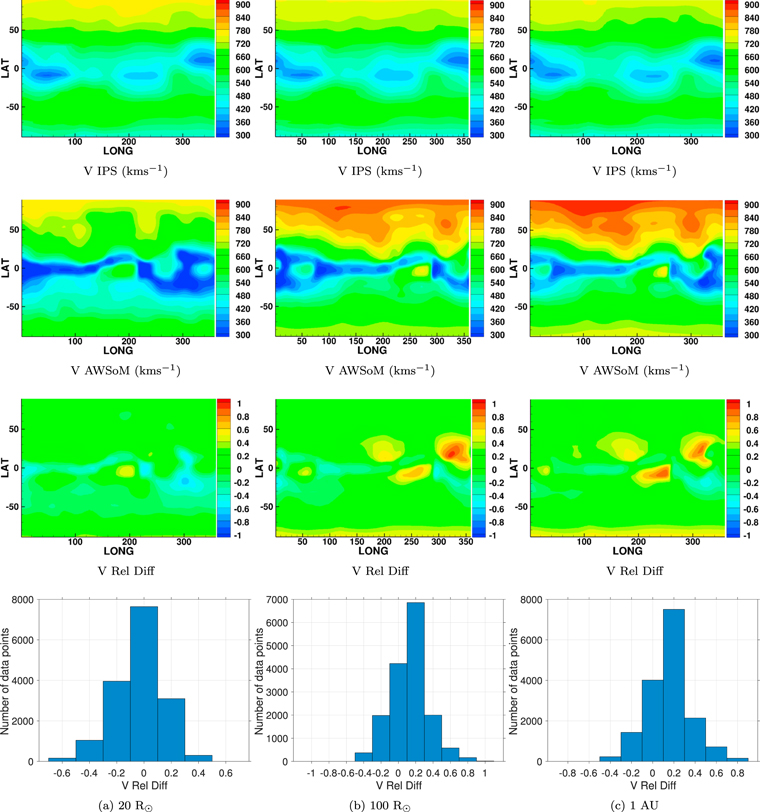
Figure 14. Comparison of reconstructed IPS velocity with AWSoM model simulations for CR 2208 at three radial distances. The three columns correspond to results at (a) 20  , (b) 100
  , and (c) 1 au respectively. The following quantities are shown in each succeeding row—IPS reconstructed solar wind velocity in kms−1 (V IPS), AWSoM predicted velocity in kms−1 (V AWSoM), relative velocity difference between IPS observations and model output, V Rel Diff =
  , and the histogram which shows how the relative difference is distributed.
Download figure:
Standard image High-resolution image
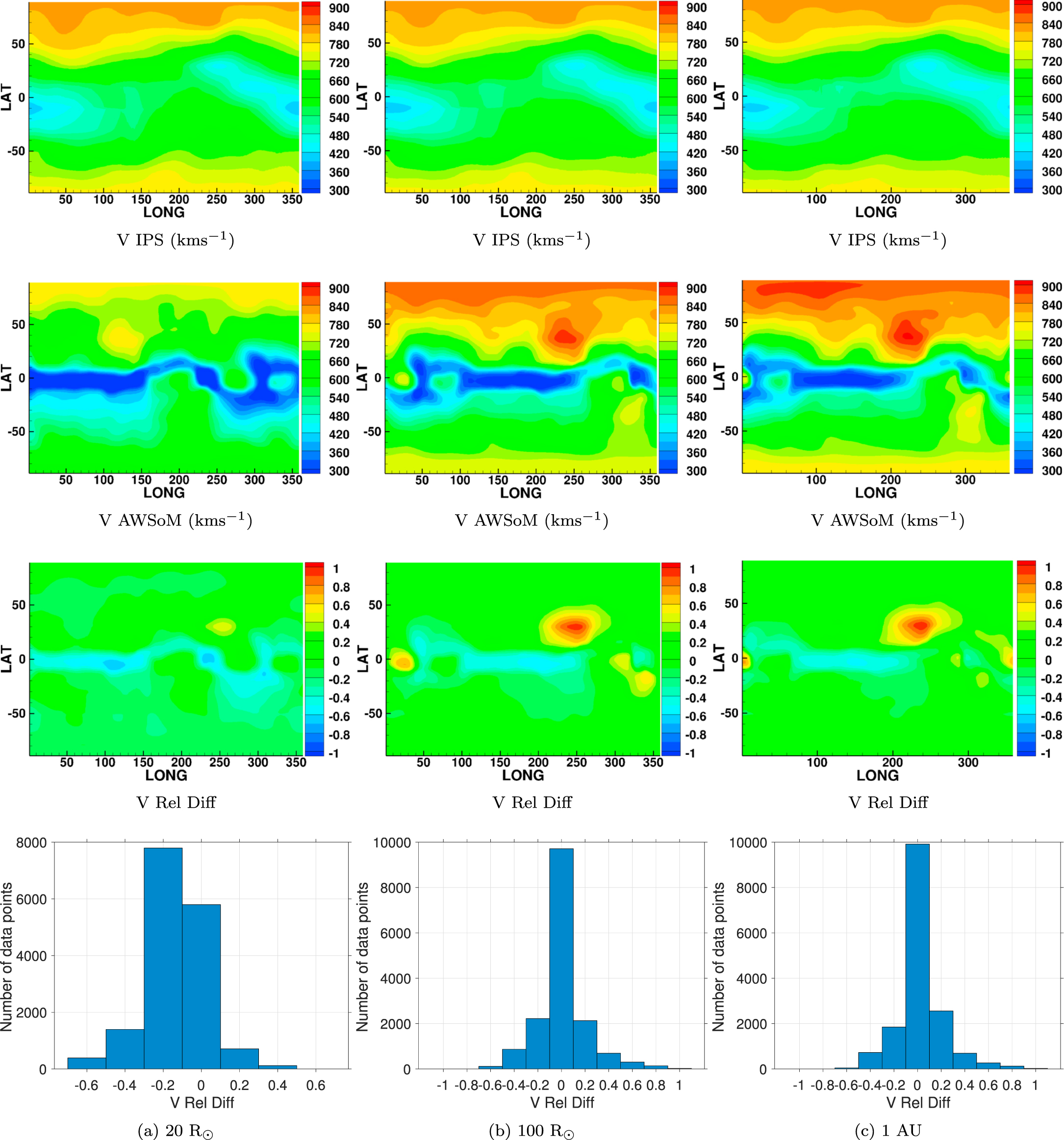
Figure 15. Comparison of reconstructed IPS velocity with AWSoM model simulations for CR 2209 at three radial distances. The three columns correspond to results at (a) 20  , (b) 100
  , and (c) 1 au respectively. The following quantities are shown in each succeeding row—IPS reconstructed solar wind velocity in kms−1 (V IPS), AWSoM predicted velocity in kms−1 (V AWSoM), relative velocity difference between IPS observations and model output, V Rel Diff =
  and the histogram which shows how the relative difference is distributed.
Download figure:
Standard image High-resolution imageThe IPS data shown here is averaged over the entire Carrington rotation for each radial distance. Data from remotely sensed IPS is the best near the Earth, since this is where the lines of sight emanate from, and the resolution of the tomography is only about 20degr × 20degr in longitude and latitude. Therefore, the analysis gets worse away from Earth. The analysis fits the in situ observations at Earth, but the OMNI data uses a mix of DSCOVR and ACE data, and sometimes these data sets differ greatly from one or another even at these low resolutions by a factor of 2 or sometimes more (Lugaz et al. 2018).
3.5. OMNI Data
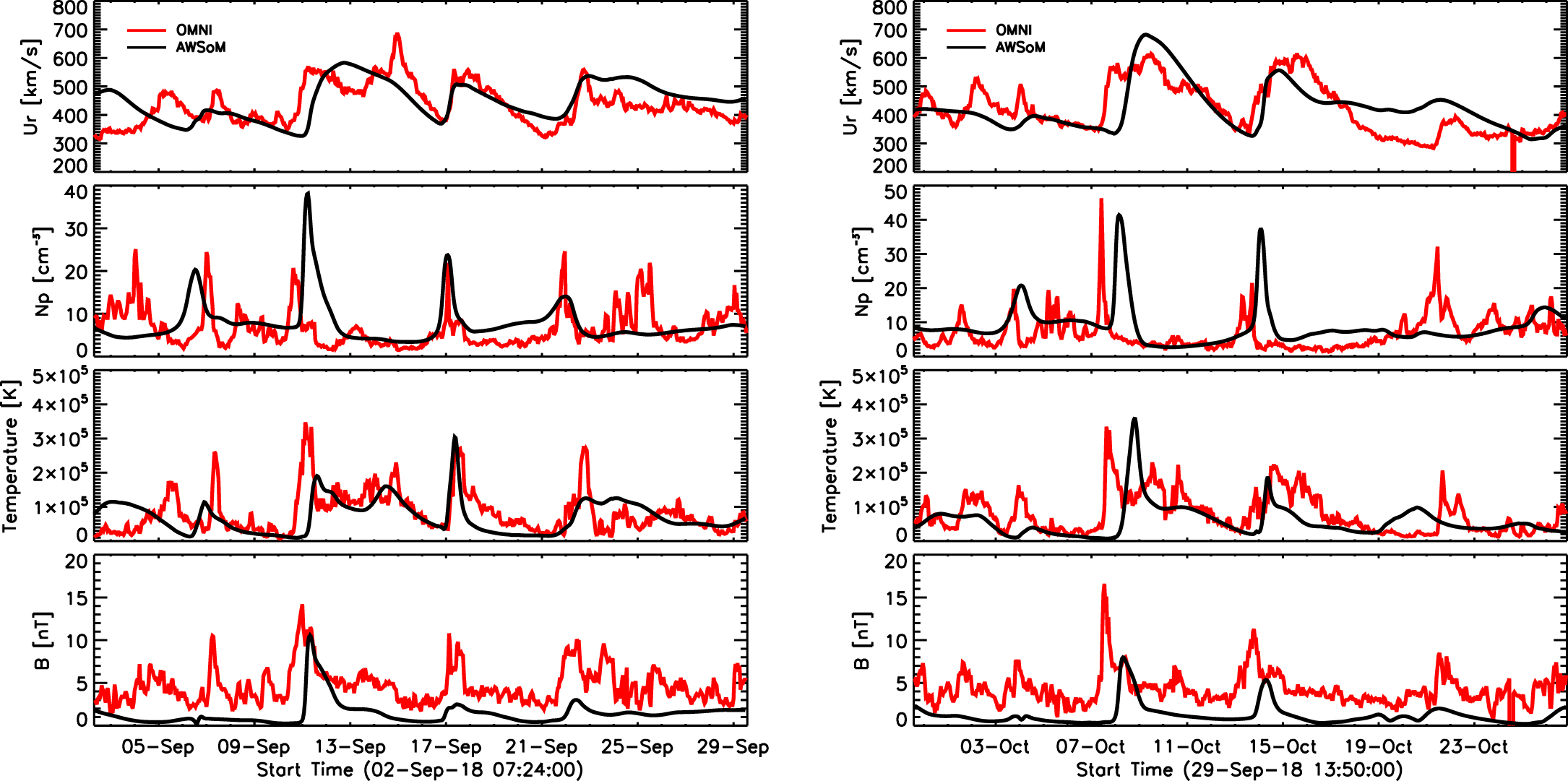
We compare the model predicted solar wind properties at 1 au with satellite observations using data from the OMNI database of the National Space Science Data Center. Figure 16 shows the comparisons of simulation results at 1 au for CR 2208 and CR 2209 with the hourly averaged OMNI data. The observation data set consists of near-Earth solar wind magnetic field and plasma parameter in situ data measured by several missions in L1 (Lagrange point) orbit. These spacecraft include the Advanced Composition Explorer (ACE), WIND, and Geotail. The spatial distance between the location of the L1 point and the Earth is taken to be negligible on heliospheric scales. Figure 16 shows the comparison of radial flow speed (Ur), proton number density (Np), proton temperature, and magnetic field strength (B) from OMNI data (red) with the AWSoM predicted results (black) at the end of the solar corona–inner heliosphere simulations. We find that the model successfully reproduces the observed solar wind conditions at 1 au. Most of the peaks in density, temperature, and magnetic field are successfully reproduced. The AWSoM results systematically overestimate the proton density for both Carrington rotations and underestimate the magnetic field. However, the overall flow speeds match reasonably well with the observations. The model also reproduces the corotating interaction regions (CIRs) represented as peaks in the density and temperature parameters quite well.

Figure 16. OMNI data (red) and AWSoM simulated solar wind parameters based on one realization of the ADAPT maps (black) at 1 au for CR 2208 (left) and CR 2209 (right).
Download figure:
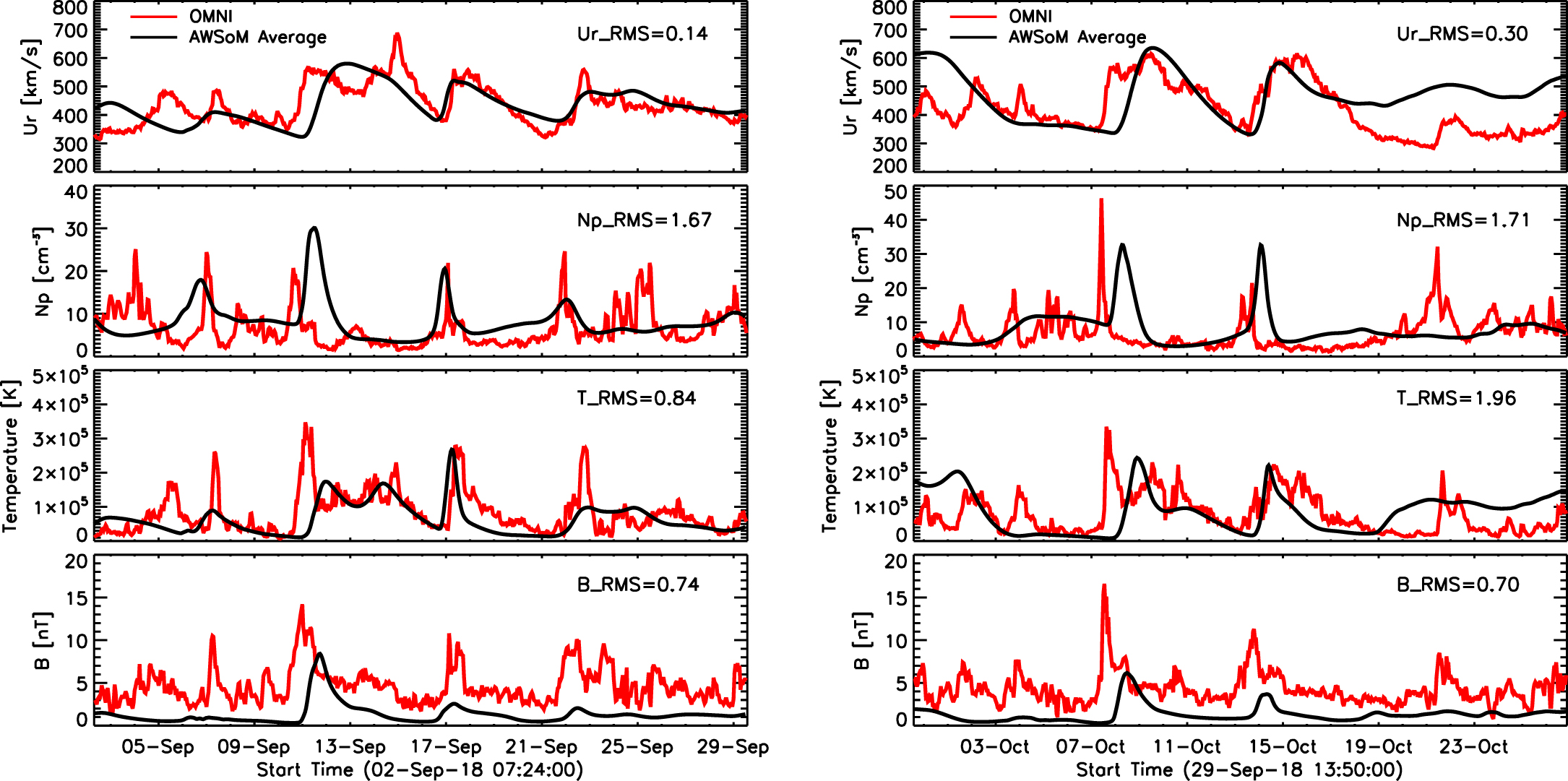
Standard image High-resolution imageADAPT–GONG maps have multiple realizations of the global magnetic field maps. For each rotation, the simulation results shown in Figure 16 are based on one realization of the ADAPT–GONG maps (shown in Figure 2). Figure 17 displays the comparison of the OMNI data (red) with the average of simulations using all 12 realizations of the ADAPT–GONG maps (black). To quantify the uncertainty in the simulation results due to the different realizations of the ADAPT maps, each panel in Figure 17 indicates the root-mean-square (rms) error between the observed (OMNI data) and the average of the simulation results using all 12 realizations of the ADAPT–GONG maps for each of the rotations. For each observed plasma parameter q, we calculate the relative rms error as
where  denotes the average of the simulation results based on all 12 ADAPT–GONG realizations. The plot shows OMNI data (red) and the average of all ADAPT map results (black) for all plasma parameters. The small rms values indicate that our model fits the observations quite well. Figure 18 shows the comparison of the OMNI data (red) to the results of the AWSoM model runs based on all 12 realizations of the ADAPT maps (gray), individually. An increase in the ensemble velocity spread is typically because of different current sheet crossing times between the realizations; that is, when the current sheet has a notable north–south alignment. However, there can also be periods when the current sheet is very close to the ecliptic. Most of the difference within the ensemble is driven by the poles, which can greatly influence the current sheet position.

Figure 17. Simulation results averaged over all realizations of ADAPT–GONG maps (black) compared with OMNI observations (red) at 1 au. The corresponding RMSE values for each parameter are informed in each panel for both CR 2208 and CR 2209.
Download figure:
Standard image High-resolution image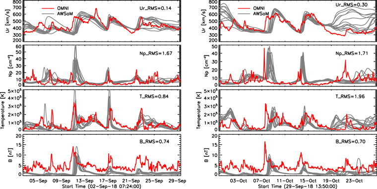
Figure 18. Simulation results from all 12 realizations of ADAPT maps (gray) compared with OMNI observations (red) at 1 au for both CR 2208 and CR 2209.
Download figure:
Standard image High-resolution imageIn general, the rms error,
between model results q1(t) and observations q2(t) over a time period T can be misleading if the curves have sharp peaks and are shifted relative to each other in time. Here q corresponds to one of the quantities of interest: density, velocity, temperature, or magnetic field. For example, in Figure 16, while the data and model results look reasonably close (for a single realization), the errors can be large because the peaks in density and temperature are shifted. We have defined a measure that evaluates the deviation between model results and observations in a more intuitive manner. We define a distance D between two curves in a plane that is independent of the coordinate system, so that the temporal and amplitude errors are treated the same way:

Here D1,2 is the average of the minimum distance between two curves integrated along curve 1:
where l1 and l2 are the coordinates along the two curves described by the (x1, y1)(l1) and (x2, y2)(l2) functions. The lengths of the curves are L1 and L2. D2,1 is defined similarly as the average minimum distance integrated along curve 2, so that D is a symmetric function of the two curves. Since time and the quantities of interest have different physical units, one needs to normalize them to the x and y coordinates. We choose X = 10 days as the normalization for time and Y = max(q) − min(q) for the normalization of quantity q, so that x = t/X and y = q/Y. This means that a time shift of 10 days is considered to be as bad as the difference between the smallest and largest amplitudes. We will use the above defined distance D to characterize the error between the observations and a particular model run.
The left panel of Figure 19 plots the errors D between the OMNI observations and the AWSoM model results for each plasma parameter for all 12 ADAPT–GONG map realizations for CR 2208 (black) and CR 2209 (red). Tables 1 and 2 list the correlation values between the errors of all parameter pairs for CR 2208 and CR 2209, respectively. We find that the distances D for solar wind velocity (Ur), temperature (T), and density (Np) are strongly correlated within each Carrington rotation; in other words the success or failure of the model in reproducing these parameters is highly correlated. Interestingly, the errors of these three plasma parameters do not correlate with the magnetic field error. We do not find a strong correlation between the errors of the corresponding ADAPT map realizations for the two consecutive Carrington rotations either, as shown in Table 3. That is, based on the two rotations that we study in this work, it cannot be said with any certainty that a particular ADAPT realization in one rotation that produces the best results will also be the best choice for a subsequent rotation.

Figure 19. Left panel: distance D between observations and model results for each ADAPT map realization for both CR 2208 (black) and CR 2209 (red). Right panel: OMNI data (red) and AWSoM simulated solar wind parameters at 1 au for CR 2208 using GONG magnetogram (cyan) and the "best" ADAPT–GONG map (black) as inputs.
Download figure:
Standard image High-resolution image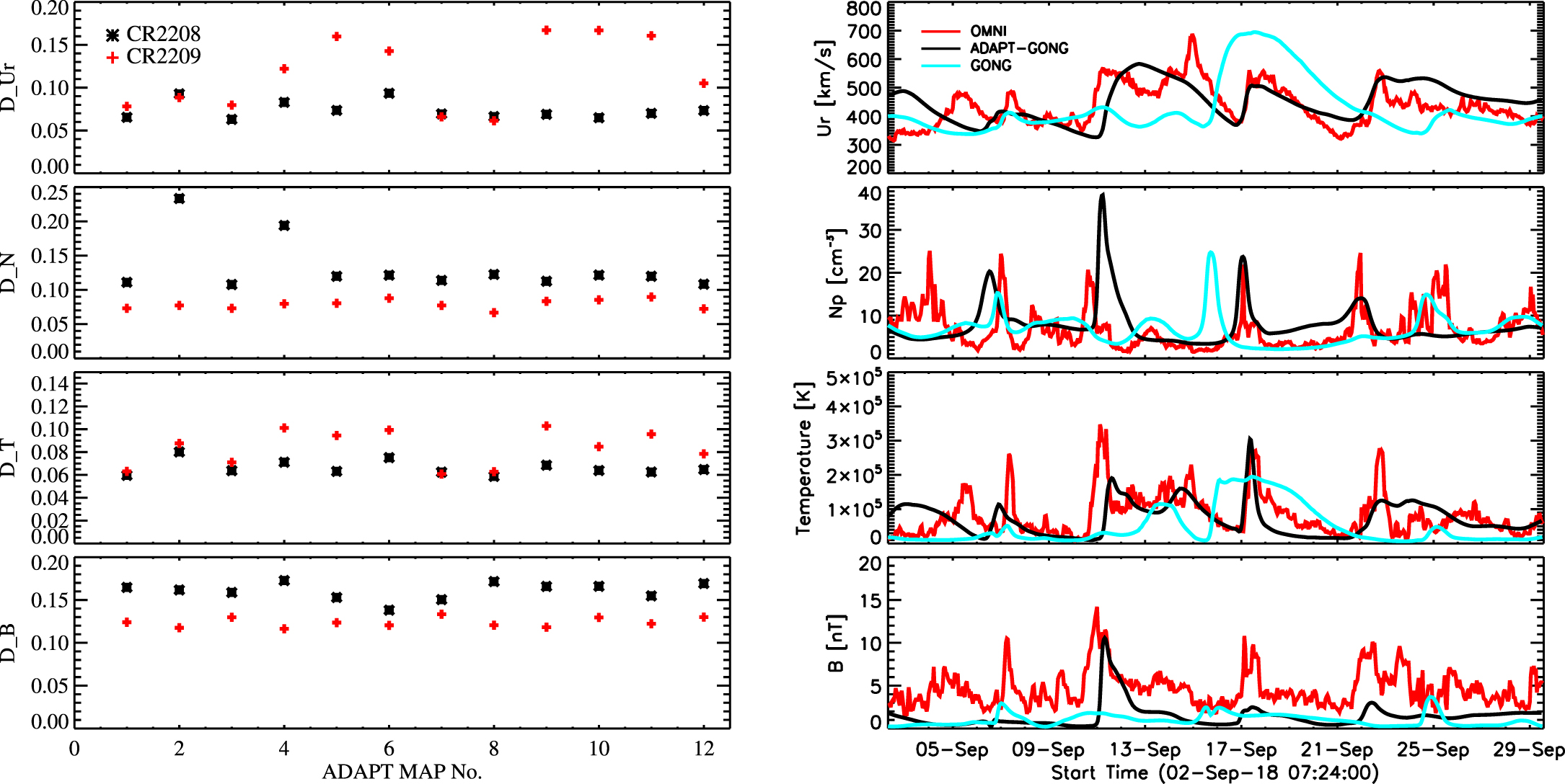
Table 1. Correlation for Errors (D) between Solar Wind Parameters for CR 2208
| CR 2208 | Np | T | B |
|---|---|---|---|
| Ur | 0.69 | 0.89 | −0.36 |
| Np | ⋯ | 0.74 | 0.22 |
| T | ⋯ | ⋯ | −0.22 |
Download table as: ASCIITypeset image
Table 2. Correlation for Errors (D) between Solar Wind Parameters for CR 2209
| CR 2209 | Np | T | B |
|---|---|---|---|
| Ur | 0.84 | 0.83 | −0.25 |
| Np | ⋯ | 0.75 | −0.19 |
| T | ⋯ | ⋯ | −0.60 |
Download table as: ASCIITypeset image
Table 3. Correlation for Errors between CR 2208 and CR 2209
| Ur | Np | T | B |
|---|---|---|---|
| 0.11 | 0.59 | 0.01 | −0.16 |
Download table as: ASCIITypeset image
Finally, we compare the performance of AWSoM with ADAPT–GONG map and GONG synoptic map. The right panel of Figure 19 shows the 1 au OMNI data (red) comparisons of simulation results for CR 2208 using GONG synoptic map (cyan) and one realization of the ADAPT–GONG synchronic map (black). It is clearly seen that by using the ADAPT–GONG maps AWSoM is able to capture much more faithfully many features of the observational data time series at 1 au, which is its ultimate goal.
4. Summary and Discussion
In this study, we show the AWSoM simulation results for CR 2208 and CR 2209 (representing solar minimum conditions) and compare them to observations. The simulations cover the domain from the solar chromosphere to the 1 au heliosphere. We compare our simulation results with a diverse set of observations ranging from low corona, into the inner heliosphere up to 1 au. These multispacecraft observations include data from SDO/AIA and STEREO-A/EUVI near the Sun, SOHO/LASCO, IPS, and OMNI. As a result, we show comparisons at various heliocentric distances from as low as 1.055–1.205  using EUV tomographic data, at 4 and 5
  using LASCO tomographic reconstructions, at 20
  , 100
, 100  , and 1 au using IPS reconstructions along with OMNI data at 1 au. The key features of AWSoM include the following: (1) Nonlinear interaction of forward propagating and partially reflected Alfvén waves leading to coronal heating due to turbulent cascade dissipation. The balanced turbulence at the apex of the closed field lines is also accounted for. (2) The model allows for anisotropic ion temperatures and isotropic electron temperature. (3) It uses the linear wave theory and nonlinear stochastic heating (Chandran et al. 2011) to distribute the turbulence dissipation to the coronal heating of these three temperatures. (4) For the isotropic electron temperature, the collisionless heat conduction is also included. There are no ad hoc heating functions.
In the past, HMI and GONG maps were used to provide the magnetic field input to the solar wind models. Here, we use the ADAPT–GONG maps, which are obtained by data assimilation that includes physical transport processes on the Sun. As a result, ADAPT maps provide more realistic estimates of the photospheric magnetic fields especially in the polar regions. We find that near the Sun, the location and extent of coronal holes and active regions are reproduced reasonably well by the model as shown in the synthesized EUV images. The average brightness of the synthetic and observed EUV images are also comparable.
Moving outwards into the corona, we compare our model to 3D DEMT reconstructions of the coronal density and temperature. Here, we find that at the lowest heights (r ≈ 1.025  ), the predicted density is elevated as an artificial extension of the transition region. However, we get excellent agreement (within ±30%) for electron density and temperature at heights above 1.055
  . At heights r = 4
  and 5
and 5  , we compare the model with the 3D electron density provided by SRT using LASCO-C2 observations. Here, we find AWSoM densities accurately match the reconstructions in the northern hemisphere, while the southern hemisphere densities are significantly higher. Further into the heliosphere, the solar wind speed predicted by our model is found to be within ±20% of the IPS reconstructed speeds at 20
  , 100
, 100  , and 1 au.
We show the plasma parameters as predicted by our model for each of the ADAPT–GONG realizations used as input. For both Carrington rotations, the proton density and temperature and solar wind speed are well-predicted by the model. However, we see that the magnetic fields are underestimated (Linker et al. 2017), and contrary to observations, the solar wind continues to accelerate in the inner heliosphere, even up to 1 au. This may be due to an overestimation of wave energy in our model. Suzuki & Inutsuka (2006) describe the Alfvén wave dissipation by addressing the mode conversion of Alfvén waves into slow (magnetoacoustic) waves. In our present model, we do not include this mode conversion and put the energy back into Alfvén waves. This can result in excess Alfvén wave energy which can lead to too much acceleration of the solar wind in the inner heliosphere.
We have shown the success of our model in reproducing the solar minimum conditions throughout the corona and inner heliosphere. These encouraging results with the AWSoM model show it to be a valuable tool to simulate solar minimum conditions. This work represents the achievement of the theoretical turbulence-based model, where self-consistent treatment of the physical processes can reproduce coronal and heliospheric observations over a tremendous range of conditions spanning orders of magnitude in density, temperature, and field strength. While this work describes the solar minimum conditions, our next validation work will focus on solar maximum conditions.
This work was primarily supported by the NSF PRE-EVENTS grant No. 1663800. W.M. was supported by NASA grants 80NSSC18K1208, NNX16AL12G, and 80NSSC17K0686. We acknowledge high-performance computing support from Cheyenne (doi:10.5065/D6RX99HX) provided by NCAR's Computational and Information Systems Laboratory, sponsored by the National Science Foundation and Frontera from NSF. W.M. acknowledges the NASA supercomputing system Pleiades. This work utilizes data produced collaboratively between Air Force Research Laboratory (AFRL) and the National Solar Observatory. The ADAPT model development is supported by AFRL. B.J. and H.-S.Y. thank M. Tokumaru and the ISEE, Japan, IPS group for making their data available for use in comparisons. B.J. is funded by NASA LWS grant 80NSSC17K0684 and AFOSR FA9550-19-1-0356 to UCSD. D.G.Ll. acknowledges CONICET doctoral fellowship (Res. Nro. 4870) to IAFE that supported his participation in this research. A.M.V. acknowledges ANPCyT grant 2012/0973 to IAFE that partially supported his participation in this research.