


Abstract
We present visible-light and ultraviolet (UV) observations of the supernova PTF 12glz. The SN was discovered and monitored in the near-UV and R bands as part of a joint GALEX and Palomar Transient Factory campaign. It is among the most energetic SNe IIn observed to date (≈1051 erg). If the radiated energy mainly came from the thermalization of the shock kinetic energy, we show that PTF 12glz was surrounded by ∼1 M⊙ of circumstellar material (CSM) prior to its explosive death. PTF 12glz shows a puzzling peculiarity: at early times, while the freely expanding ejecta are presumably masked by the optically thick CSM, the radius of the blackbody that best fits the observations grows at ≈7000 km s−1. Such a velocity is characteristic of fast moving ejecta rather than optically thick CSM. This phase of radial expansion takes place before any spectroscopic signature of expanding ejecta appears in the spectrum and while both the spectroscopic data and the bolometric luminosity seem to indicate that the CSM is optically thick. We propose a geometrical solution to this puzzle, involving an aspherical structure of the CSM around PTF 12glz. By modeling radiative diffusion through a slab of CSM, we show that an aspherical geometry of the CSM can result in a growing effective radius. This simple model also allows us to recover the decreasing blackbody temperature of PTF 12glz. SLAB-Diffusion, the code we wrote to model the radiative diffusion of photons through a slab of CSM and evaluate the observed radius and temperature, is made available online.
Export citation and abstract BibTeX RIS
1. Introduction
Type IIn supernovae (SNe) are characterized by prominent and narrow-to-intermediate width Balmer emission lines in their spectra (Schlegel 1990; Filippenko 1997; Smith 2014; Gal-Yam 2017). Rather than a signature of the explosion itself, this spectral specificity is presumably the result of the photoionization of a dense, hydrogen-rich, circumstellar medium (CSM) that is ejected from the SN progenitor prior to the explosion.
The Type IIn class is not a well-defined category of objects, as many SNe show the characteristic narrow Balmer lines in their spectra, sometime during their evolution. These lines are the signature of an external physical phenomenon highly dependent on the surrounding environment, rather than of any intrinsic property of the explosion. Depending on the spatial distribution and physical properties of the CSM, these lines may persist for days ("flash spectroscopy," Gal-Yam et al. 2014; Khazov et al. 2016; Yaron et al. 2017), weeks (e.g., SN 1998 s, Li et al. 1998; Fassia et al. 2000, 2001; SN 2005gl, Gal-Yam et al. 2007; SN 2010mc, Ofek et al. 2013a), or years (e.g., SN 1988Z, Danziger & Kjaer 1991; Stathakis & Sadler 1991; Turatto et al. 1993; van Dyk et al. 1993; Chugai & Danziger 1994; Fabian & Terlevich 1996; Aretxaga et al. 1999; Williams et al. 2002; Schlegel & Petre 2006; Smith et al. 2017; 2010 jl, Patat et al. 2011; Stoll et al. 2011; Gall et al. 2014; Ofek et al. 2014a).
In the last decades, the physical picture governing SN IIn explosions and the wider family of "interacting" SNe—SNe whose radiation can be partially or completely accounted for by the ejecta crashing into a dense surrounding medium—has become clearer (see, e.g., Chevalier 1982; Chugai & Danziger 1994; Chugai et al. 2004; Ofek et al. 2010; Chevalier & Irwin 2011; Ginzburg & Balberg 2014; Moriya & Maeda 2014). In recent years, there has been growing evidence that, in the majority of cases, the high-density CSM originates from explosive phenomena taking place in the months to years prior to the SN explosion. One piece of evidence supporting this conclusion is the direct detection of the so-called precursors (luminous outbursts) in the months to years prior to the SN explosion (e.g., Foley et al. 2007; Pastorello et al. 2007; Fraser et al. 2013; Ofek et al. 2013a, 2014b, 2016; Elias-Rosa et al. 2016; Thöne et al. 2017). Several theoretical mechanisms have been suggested to explain extreme mass-loss episodes in the final stages of stellar evolution (e.g., Woosley et al. 2007; Chevalier 2012; Quataert & Shiode 2012; Soker & Kashi 2016).
While in normal core-collapse SNe, the radiation-mediated shock breaks out upon reaching the stellar surface, producing a strong blast in the UV and X-rays (Nakar & Sari 2010; Rabinak & Waxman 2011), in the case of SNe IIn the ejecta may crash into the optically thick CSM. The radiation-dominated and radiation-mediated shock runs into the CSM surrounding the star and goes on propagating into it as long as τ ⪆ c/vsh, where τ is the optical depth from the shock to the edge of the wind, vsh is the shock velocity, and c is the speed of light (e.g., Ofek et al. 2010). When τ ∼ c/vsh (this condition is verified when the timescale for photons to diffuse from the shocked region to the photosphere becomes comparable to the dynamical timescale of the shock), the shock breaks out: photons diffuse ahead of the shock faster than the ejecta and radiation can escape ahead of the shock (Weaver 1976). After the shock breakout, in the presence of massive CSM above the shock, the radiation-dominated shock transforms into a collisionless shock (Katz et al. 2011; Murase et al. 2011, 2014). The collisionless shock slows down the ejecta and converts its kinetic energy into hard X-ray photons (Katz et al. 2011; Murase et al. 2011, 2014). If the optical depth of the CSM above the shock is high enough, the X-rays generated in the collisionless shock are converted into UV and visible radiation (e.g., Chevalier & Irwin 2012; Svirski et al. 2012). Without a sufficient optical depth, though, the bulk of the X-ray photons will not convert into optical photons.
As far as a spectral signature is concerned, the common picture explaining SNe IIn observations is as follows. As long as the CSM is optically thick, the photosphere that emits the continuum is located in the unshocked CSM, masking the observer's view of the shock. The radiation from the shock propagates upstream and photoionizes the slowly moving CSM, resulting in relatively narrow Balmer recombination emission lines in the SN spectrum. As the shock reaches the optically thin medium, broader components can appear in the spectrum—maybe arising from the shocked zone forming at the contact discontinuity between the decelerated ejecta and the shocked CSM (Chugai et al. 2004). Alternatively, if the CSM is optically thin, lines from the fast moving SN ejecta, generated in the inner regions, may become visible (e.g., Chevalier & Fransson 1994).
Observing SNe IIn at wavelengths where the collisionless shock radiates most—namely UV and X-rays—has the potential to unveil precious information about the explosion mechanism and the CSM properties (e.g., Ofek et al. 2013b). In particular, it may provide a much better estimate of the bolometric luminosity of the event. In this paper, we present and analyze the UV and visible-light observations of PTF 12glz, an SN IIn observed in a joint campaign by GALEX and the Palomar Transient Factory (PTF) and detected in the UV. PTF 12glz is one of the six SNe discovered during this campaign (Ganot et al. 2016). The survey was carried out as a proof-of-concept for the ULTRASAT mission (Sagiv et al. 2014).
Observations of SNe IIn are usually analyzed within the framework of spherically symmetric models of CSM. However, resolved images of stars undergoing considerable mass loss (e.g., η Carinae; Davidson & Humphreys 1997, 2012), as well as polarimetry observations (Leonard et al. 2000; Hoffman et al. 2008; Wang & Wheeler 2008; Reilly et al. 2017) suggest that asphericity should be taken into account for more realistic modeling. Asphericity of the CSM has recently been invoked to interpret the spectrocopic and spectropolarimetric observations of the Type IIn SN SN 2012ab (Bilinski et al. 2018) and SN 2009ip (Mauerhan et al. 2014; Levesque et al. 2014; Smith et al. 2014; Reilly et al. 2017). In this paper, we show that the light curve of PTF 12glz may be interpreted as evidence for aspherical CSM.
We present the aforementioned observations of PTF 12glz in Section 2. In Section 3, we present the analysis of these observations and the puzzling inconsistency between the spectroscopic and photometric observations. In Section 4, we model the radiative diffusion of photons through an aspherical slab and propose a solution to this puzzle. We then summarize our main results in Section 5. In the Appendix, we make available SLAB-Diffusion (Soumagnac 2018, Codebase: https://github.com/maayane/SLAB-Diffusion), a computer code for modeling radiation through a slab of CSM.
2. Observations and Data Reduction
In this section, we present the observations of PTF 12glz by the GALEX /PTF UV wide-field transient survey. This campaign, conducted during a nine-week period from 2012 May 24 through 2012 July 28, used the GALEX NUV camera to cover a total area of about 600 deg2 over 20 times with a three-day cadence, while PTF observed the same region with a two-day cadence (Ganot et al. 2016).
2.1. Discovery
PTF 12glz was discovered on 2012 July 7 by the PTF (Law et al. 2009; Rau et al. 2009) automatic pipeline reviewing potential transients in the data from the PTF camera mounted on the 1.2 m Samuel Oschin telescope (P48, Rahmer et al. 2008). The image processing pipeline is discussed in Laher et al. (2014) and the photometric calibration is described in Ofek et al. (2012). The SN is associated with an r = 18.51 mag galaxy, SDSS13
J155452.95+033207.5, shown in Figure 1 and modeled in Section 3.2. The coordinates of the object, measured in the PTF images are α = 15h54m53 04, δ = +03d32
 07
07 5 (J2000.0). The redshift z = 0.0799 and the distance modulus μ = 37.77 were obtained from the spectrum and the extinction was deduced from Schlafly & Finkbeiner (2011) and using the extinction curves of Cardelli et al. (1989). All these parameters are summarized in Table 1.

Figure 1. Top panels: (left to right) the discovery image, reference image, and subtracted P48 image of PTF 12glz. Lower panel: the SDSS image of J155452.95+033207.5, the host of the supernova PTF 12glz. The box encircles the host: α = 238 72100 and δ = 353542. Credit: SDSS.
Download figure:
Standard image High-resolution imageTable 1. Summary of PTF 12glz Observational Parameters
| Parameter | Value |
|---|---|
| R.A. α (J2000) | 238721000 |
| Decl. δ (J2000) | 3535421 |
| redshift z | z = 0.0799 |
| distance modulus μ | 37.77 mag |
| galactic extinction EB−V | 0.13 mag |
Download table as: ASCIITypeset image
Previous PTF observations were obtained in the years prior to the SN explosion, but no previous detection of any precursor outburst exists. The most recent nondetection was on 2012 June 25. We present a derivation of the explosion epoch in Section 3.4.
2.2. Photometry
PTF 12glz was observed in multiple bands for almost three years after discovery. The SN was monitored during a rising phase (t < 36 days) and a decay phase (t > 243 days) but not around peak luminosity. All the host-subtracted light curves are shown in Figure 2. The photometry is reported in electronic Table 2 and is available via WISeREP.14
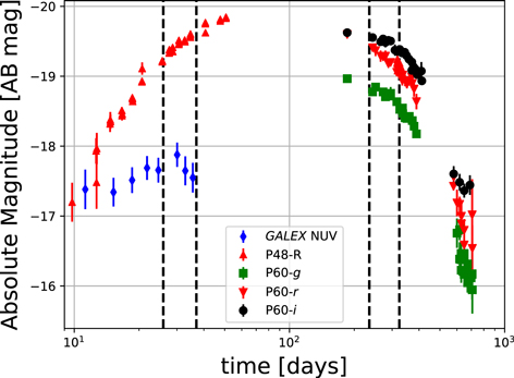
Figure 2. Light curve of PTF 12glz. Time is shown relative to the estimated epoch at which the extrapolated light curve (Equation (1)) is crossing zero: t0 = 2456097.58 (2012 June 19), as derived in Section 3.4. Black dashed lines indicate dates at which spectroscopic data exist.
Download figure:
Standard image High-resolution imageTable 2. Photometry
| Epoch (days) | Counts (arb.) | Mag (magAB) | Instrument |
|---|---|---|---|
| 11.24 | 0.75 ± 0.13 | 20.38 ± 0.28 | GALEX nUV |
| 9.71 | 362.30 ± 86.30 | 20.60 ± 0.26 | P48/R |
| 185.48 | ⋯ | 19.01 ± 0.06 | P60/g' |
| 185.48 | ⋯ | 18.85 ± 0.04 | P60/r' |
| 185.48 | ⋯ | 18.40 ± 0.05 | P60/i' |
Note. Time is shown relative to the estimated epoch at which the extrapolated light curve (based on Equation (1)) is crossing zero: t0 = 2456097.58 (2012 June 19), as derived in Section 3.4. To compute the apparent magnitudes from the counts, the zero-point for the nUV data is ZPnUV = 20.08 and the zero-point for the P48 data is ZPP48 = 27.00.
Only a portion of this table is shown here to demonstrate its form and content. A machine-readable version of the full table is available.
Download table as: DataTypeset image
GALEX observations of the PTF 12glz field started on 2012 May 26 and 15 observations were obtained with a cadence of ∼3 days. The GALEX NUV camera was operating in scanning mode and observed strips of sky in a drift-scan mode with an effective average integration time of 80 s, to an NUV limiting magnitude of 20.6 mag [AB]. The GALEX data reduction was done using tools15 by Ofek (2014).
The P48 telescope was used with a 12K × 12K CCD mosaic camera (Rahmer et al. 2008) and a Mould R-band filter. Data were obtained with a cadence of ∼2 days, to a limiting magnitude of R ≈ 21 mag [AB]. For the data reduction of the P48 data, we used a pipeline developed by Mark Sullivan (Sullivan et al. 2006; Firth et al. 2015).
The robotic 1.52 m telescope at Palomar (P60; Cenko et al. 2006) was used with a 2048 × 2048 pixel CCD camera and g', r', i' SDSS filters. Data reduction of the P60 data was performed using the FPipe pipeline (Fremling et al. 2016). We calibrated the P60 data in the following way. The r-band light curve was scaled so that its average value during the time window covered by both telescopes matches the average value of the P48 R-band photometric data. The g-band and i-band data were scaled to match the synthetic photometry of the calibrated spectroscopic data (Section 2.3). The synthetic photometry used for the calibration and for other purposes in this paper was computed with the PyPhot16 pipeline (M. Fouesneau 2019, in preparation).
Although the photometric data available for PTF 12glz do not cover the peak, the data during the rise and decay allow us to place an upper limit on the absolute magnitude at peak: with Mr ≲ −20, PTF 12glz is at the bright end of the observed SNe IIn, together with, e.g., SN 2006gy (Ofek et al. 2007; Smith & McCray 2007), SNe 2008fq (Thrasher et al. 2008; Taddia et al. 2013), or SN 2003ma (Rest 2009; Rest et al. 2011). In particular, it is brighter than all SNe in the sample by Kiewe et al. (2012), which was designed to be unbiased.
2.3. Spectroscopy
Four optical spectra of PTF 12glz were obtained using the telescopes and spectrographs listed in Table 3. The two first spectra were taken during the light-curve rise, and the two last ones during the decay, at the dates shown in Table 3. The spectra were used to determine the redshift z = 0.0799 from the narrow host lines (Hα and [O iii]). All the observations were corrected for a galactic extinction of EB−V = 0.13 mag, deduced from Schlafly & Finkbeiner (2011) and using Cardelli et al. (1989) extinction curves, with the parameter R ≡ A(V)/EB−V (i.e., the ratio of total to selective extinction at V) set to the value R = 3.1. In Section 3.3, we show that our qualitative results are not affected when varying R, e.g., within the interval given in Fitzpatrick (1999).
Table 3. Spectroscopic Observations of PTF 12glz
| Date | Phase | Facility | Reference |
|---|---|---|---|
| 2012 Jul 15 | +26.2 days | P200 | Oke & Gunn (1982) |
| 2012 Jul 26 | +36.9 days | P200 | ⋯ |
| 2013 Feb 9 | +235.1 days | LRIS | Oke et al. (1994) |
| 2013 May 9 | +324.0 days | LRIS | ⋯ |
Note. The phase is given from the explosion epoch derived in Section 3.4. The double-beam spectrometer (Oke & Gunn 1982) mounted on the 200'' Hale telescope at Palomar was used with a 1'' slit, the 5500 Å dichroic and the 316/7150 grating positioned at a grating angle of 24° 38.2 minutes. The Low-Resolution Imaging Spectrometer (LRIS; Oke et al. 1994) spectrometer mounted on the 10 m Keck I telescope was used with a 1'' slit, the 5600 Å dichroic and the 400/3400 grism on the blue side.
Download table as: ASCIITypeset image
The spectroscopic observations were calibrated in the following way: the first two and the last spectra, for which we have contemporaneous P48 R-band data, were scaled so that their synthetic photometry matches the P48 R-band value. The third spectrum was scaled in the same way using the overlapping P60 r-band data instead.
The first and last spectra are shown in Figure 3 (the first two spectra are very similar, as well as the last two spectra) and all spectra are available from the Weizmann Interactive Supernova data REPository17 (WISeREP, Yaron & Gal-Yam 2012).

Figure 3. Earliest (top) and latest (bottom) observed spectra of PTF 12glz. Both spectra were calibrated to the R-band photometric measurement. Dashed lines indicate the redshifted emission lines for the Balmer series. Black stars show the combination of the observed (NUV and P48 R-band) and synthetic (g, r, and i sdss bands) photometry. The dashed red line shows the blackbody curves that best fit the photometric data (and the best-fit values are shown in the box with dashed contours), while the green continuous line shows the blackbody curve that best fits the spectroscopic data (and the best-fit values are shown in the box with dashed contours).
Download figure:
Standard image High-resolution image
Figure 4. Hα line profile on 2012 July 15 (earliest spectrum). The bold black line shows the observed spectrum. The red dotted line and blue dashed line are the narrow Gaussian (G) and intermediate-width Lorentzian (L) whose linear combination (gray continuous line) best fits the data. The origin of the x-axis indicates the location of the Hα line at the host galaxy, at redshift z = 0.0799. The vertical lines indicate the center of each component: the narrow component is blueshifted by ∼−30 km s−1 and the intermediate-width component is blueshifted by ∼−50 km s−1.
Download figure:
Standard image High-resolution image3. Analysis
3.1. Spectroscopy
The two early spectra, obtained during the rise of the light curve, are characteristic of interacting SNe: a blue continuum with strong and narrow Balmer lines, as well as weak He i (5876, 7065 Å) narrow lines. At short wavelengths, the spectra show absorption from iron, as seen, for example, in SN 2010jl.18
We fitted a blackbody spectrum to the six-point spectral energy distribution (SED) (corrected for redshift and extinction) obtained by combining (1) the observed photometry in the NUV and P48 R-band (2) the synthetic photometry of the spectra in the g, i and r SDSS bands. The best-fit temperatures and radii are shown in Table 4 and Figure 7 (as stars). In Figure 3, we show the synthetic and observed photometry derived for the earliest spectrum, on which is superimposed the calibrated spectrum and the best blackbody fit.
Table 4. The Table shows the Best-fit Values of the Continuum and Hα Lines in the Four Spectra of PTF 12glz
| Date | Continuum | Hα narrow comp. | Hα intermediate comp. | Hα broad comp. | ||||
|---|---|---|---|---|---|---|---|---|
| TBB | RBB | Δv | FWHM | Δv | FWHM | Δv | FWHM | |
| (K) | (1015 cm) | (km s−1) | (km s−1) | (km s−1) | (km s−1) | (km s−1) | (km s−1) | |
| 2012 Jul 15 |

|

|
−35 | 110 | −50 | 680 | ⋯ | ⋯ |
| 2012 Jul 26 |

|

|
−80 | 240 | −100 | 530 | ⋯ | ⋯ |
| 2013 Feb 09 |

|

|
⋯ | ⋯ | −270 | 1990 | −1070 | 8580 |
| 2013 May 09 |

|

|
⋯ | ⋯ | −240 | 2310 | −830 | 7470 |
Note. The early spectra are best fit with a linear combination of a narrow Gaussian component (left column) and an intermediate-width Lorentzian component (central column). The late spectra are best fit with a linear combination of an intermediate-width Gaussian component (central column) and a broad Gaussian component (right column). Δz is the shift of the center of each component compared to the galaxy rest frame (the negative values mean that the component is blueshifted).
Download table as: ASCIITypeset image
Both early spectra show strong and narrow Balmer lines, which for SNe IIn are interpreted as coming from the slow, unshocked, photoionized CSM. Their broad Lorentzian wings may be the signature of electron scattering, as the Hα photons diffuse ahead of the shock through the dense CSM (e.g., Chugai 2001). After subtracting the best-fit continuum from the spectra, we fitted the narrow Hα lines. We tried several linear combinations of Gaussian and Lorentzian functions: the best fit is a superposition of a narrow Gaussian component with FWHM ≈ 100–200 km s−1 (i.e., unresolved), which we interpret as tracing the slow unshocked CSM and an intermediate Lorentzian component with FWHM ≈ 500–700 km s−1 (if some of the line-broadening comes from electron scattering, this is an upper limit of the CSM speed). The derived speeds and offsets are shown in Table 4. Figure 5 shows the line and the best fit for the latest spectrum.

Figure 5. Hα line profile on 2013 May 09 (latest spectrum). The bold black line shows the observed spectrum. The red dotted line and blue dashed line are the intermediate-width and broad Gaussian (G) components whose linear combination (in gray) best fits the data. The vertical lines indicate the center of each component: the narrow component is blueshifted by ≈−230 km s−1 and the intermediate-width component is blueshifted by ≈−830 km s−1.
Download figure:
Standard image High-resolution imageNo signature of expanding material is visible in the spectrum at this stage, which is consistent with a thick CSM obstructing the view of the SN ejecta at early times. We will show in Section 3.3 how the photometric data are inconsistent with this picture.
The fits mentioned above, as well as all those mentioned in the rest of this paper, were performed using the emcee algorithm (Foreman-Mackey et al. 2013) to sample from the posterior probability distribution. We then used the 10 combinations with the lowest χ2 from the Markov chain Monte Carlo as initial conditions for an optimization algorithm to compute the best-fit value (the maximum a posteriori value or "m.a.p.," in the terminology of Hogg et al. 2010). Note that we used MCMC to compute the posterior distribution and deduce the error bars on the one hand and, on the other hand, used a distinct optimization algorithm to solve for the set of parameters maximizing the posterior, i.e., find the m.a.p. (which coincides with the maximum likelihood value and the minimum χ2 value because the priors are uninformative). The reason we took this precaution—which turned out to be unnecessary—is that in the case of non-Gaussian or nonsymmetric marginalized posterior distribution, the m.a.p. may not fall necessarily close to the median of the posterior distribution. In such cases, computing the position of the m.a.p. can be problematic and challenging, all the more when the χ2 is noisy and full of local minima. The main challenge is then to choose an initial combination of parameter values to give a minimization algorithm (most minimization algorithms require an initial combination of parameters from which to start their search for the minimum). Here, we made the following choice of initial conditions (a reasonable yet somewhat arbitrary choice): we took the 10 sets of parameters from the chain corresponding to the lowest χ2. In the current case, because the posterior distribution is reasonably close to a Gaussian and is well-behaved, the m.a.p. coincides with the median of the posterior distribution.
When errors are noted, they correspond to the 1σ limits of the marginalized posterior distributions.
The interpretation of the late-time spectra of SNe IIn should be made with the complexity caused by CSM interaction in mind. In "normal" SNe II, the ejecta that become optically thin at late times are heated from the inside by two sources of energy: (1) remaining thermal deposition from the original heat of the explosion and (2) radioactivity. The late, or "nebular," spectrum shows no clear continuum, and its emission lines reflect the expansion of the ejecta in which they formed. In SNe IIn, the CSM interaction may continue to dominate the spectrum at late times, e.g., because the ejecta is heated by the shock wave propagating backward from the CSM into its outermost layers (Chevalier & Fransson 2003).
The two late-time spectra of PTF 12glz look similar (the latest spectrum is shown in Figure 3): they show a weak continuum in red, a pseudo-continuum presumably formed by the superposition of narrow [Fe ii] emission lines in the blue (e.g., Kiewe et al. 2012), and several broad emission lines. The temperatures and radii derived by fitting a blackbody curve to the observed spectrum are listed in Table 4 and compared to the parameters derived from photometry in Figure 7. Both spectra show broad Balmer emission lines. The derived speeds and redshifts are presented in Table 4. Figure 4 shows the line and the best fit for the earliest spectrum and Figure 5 shows them for the latest spectrum. The Hα lines are best fit by a linear combination of an intermediate-width Gaussian component with FWHM ≈ 2000 km s−1 that is offset to the blue by ≈250 km s−1 relative to the galaxy rest frame and a broad Gaussian component with FWHM ≈ 8000 km s−1 that is offset to the blue by ≈1000 km s−1 relative to the galaxy rest frame. The intermediate-width component could come from the shocked gas in a cold dense shell forming at the contact discontinuity between the decelerated ejecta and the shocked CSM, which is reheated by X-rays and UV radiation from the shock. The broad component velocities are too high to originate from the CSM: they are rather characteristic ejecta velocity values. We deduce from these velocities that the ejecta has—at least partially—emerged through the optically thick layers of the CSM.
Both late spectra also show emission from the the Ca ii IR triplet. This is commonly seen in late-time-interacting SNe, e.g., in the type IIn SN 2005ip (Boles et al. 2005; Stritzinger et al. 2012), the type Ic SN 2007dio (Kuncarayakti et al. 2018) and the type Ia-csm PTF 11kx (Dilday et al. 2012; Silverman et al. 2013; Graham et al. 2017), as well as in other types of SNe.
3.2. Host Galaxy
We retrieved science-ready imaging data from the several surveys, summarized in Table 5: the Galaxy Evolution Explorer (GALEX) general release 7 (GR7) (Martin et al. 2005), the Panoramic Survey Telescope and Rapid Response System (Pan-STARRS; PS1) data release 1 (DR1) (Flewelling et al. 2016) and the Sloan Digital sky survey data release 9 (DR9) (SDSS; Ahn et al. 2012). We used the software package LAMBDAR (Lambda Adaptive Multi-Band Deblending Algorithm in R; Wright et al. 2016) that is based on Bourne et al. (2012) to perform multiband matched aperture photometry (i.e., taking into account different pixel scales and point-spread functions). The absolute flux calibration was done against instrument-specific zero points (for details on the photometry, see S. Schulze et al. 2019, in preparation).
Table 5. Photometry of the Host Galaxy
| Instrument | Filter | Wavelength | Brightness |
|---|---|---|---|
| (Å) | (magAB) | ||
| GALEX | FUV | 1542.3 | 21.55 ± 0.46 |
| GALEX | NUV | 2274.4 | 21.23 ± 0.51 |
| SDSS | u' | 3594.9 | 19.88 ± 0.17 |
| SDSS | g' | 4640.4 | 18.59 ± 0.07 |
| SDSS | r' | 6122.3 | 17.96 ± 0.08 |
| PS1 | i' | 7439.5 | 17.75 ± 0.07 |
| SDSS | z' | 8961.5 | 17.59 ± 0.10 |
| PS1 | Y | 9603.1 | 17.23 ± 0.19 |
Note. The photometry is not corrected for Galactic reddening. The effective wavelengths were taken from the Spanish Virtual Observatory (https://svo.cab.inta-csic.es/).
Download table as: ASCIITypeset image
We modeled the SED of the host galaxy with the software packages Le Phare on the web portal GAZPAR19 (GAlaxy photometric redshifts (Z) and physical PARameters). We modeled the data using a grid of templates based on Bruzual & Charlot (2003) stellar population-synthesis models with the Chabrier initial-mass-function (Chabrier 2003), a star formation history that is approximated by a declining exponential function, and a Calzetti et al. (2000) dust attenuation curve.
Figure 6 shows the measured galaxy photometry and the best fit. The SED can be adequately described by a template with a stellar mass of  , a star formation rate of
  , and negligible attenuation
 ![$\left[E\left(B-V\right)=0\right]$](https://content.cld.iop.org/journals/0004-637X/872/2/141/revision1/apjaafe84ieqn11.gif) (χ2/number of filters = 1.3/8). Using the parameterization of the mass–metallicity relation by Andrews & Martini (2013), we estimate the galaxy metallicity to be ∼0.4–0.5 solar.
(χ2/number of filters = 1.3/8). Using the parameterization of the mass–metallicity relation by Andrews & Martini (2013), we estimate the galaxy metallicity to be ∼0.4–0.5 solar.

Figure 6. Spectral energy distributions of the host of PTF12glz from 1000 to 14000 Å. The observed magnitudes are displayed by the circles. The solid line displays the best-fit model of the SED with Le Phare. The squares are the model predicted magnitudes.
Download figure:
Standard image High-resolution image3.3. The Peculiar Evolution of the Blackbody Radius
Taking advantage of the multiple-band photometry coverage, we derived the temperature and radius of the blackbody that best fits the photometric data at each epoch (after correcting for redshift and extinction, interpolating the various data sets to obtain data coverage of coinciding epochs and deriving the errors at the interpolated points with Markov chain Monte Carlo (MCMC) simulations). The derived best-fit temperatures TBB and radii rBB are shown in Figure 7. For the temperature MCMC fit, we adopted a broad, uninformative (flat) prior T ∈ [5000, 25000]. The edge values of the prior were chosen to contain the range of temperatures observed, e.g., in the SNe IIn sample by Taddia et al. (2013). The best-fit temperatures TBB should be seen as a lower limit on the temperature, because the spectra of SNe typically show a deficit of flux due to line-blanketing by metal lines.
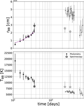
Figure 7. Evolution in time of (1) the radius (top panel) and (2) the temperature (lower panel) of a blackbody with the same radiation as PTF 12glz. The points were obtained by fitting a blackbody spectrum to the observed photometry, after interpolating the various data sets to obtain data coverage of coinciding epochs. The errors were obtained with MCMC simulations. The star symbols indicate the values derived by fitting a blackbody to the spectroscopic data. The dashed line in the top panel shows the best linear fit to the rising radius phase: a linear function with a slope of ≈7000 km s−1. At late times, the blackbody model for the spectral energy distribution may not be valid anymore (see, e.g., the right panel in Figure 3): these points are shown in gray to emphasize that they are less reliable and should be taken cautiously.
Download figure:
Standard image High-resolution imageIn most epochs, this method implies fitting a blackbody spectrum to a two-point SED. Comparison with results derived from more constraining data detailed in Section 3.1—either spectroscopy (shown in red) or a combination of observed and synthetic photometry (shown in green)—suggests that this method leads to a slight overestimation of the radius and underestimation of the temperature.
The temperature TBB drops from ≈15,000 K to ≈8000 K during the rise and is stable at ≈6000 K during the decay phase. The decrease of TBB at early times is well fitted by a power law tn with index n = −0.6 and is consistent with the temperature evolution observed in the sample by Taddia et al. (2013). However, PTF 12glz is relatively hot compared to the SNe IIn of this sample, where temperatures span between 11,500 K and 5500 K, and compared to other well studied SNe IIn (e.g., 2006gy, Ofek et al. 2007; Smith & McCray 2007; SN 2005ip, Smith et al. 2009; SN 2010jl, Ofek et al. 2014a).
The derived radius grows by an order of magnitude, from  cm to
cm to  cm during the rising phase and is ≈4 × 1015 cm during the light-curve decay phase. Such a rise is puzzling within a picture where the optically thick CSM is supposed to mask the shock and the expanding material. To our knowledge, the measured blackbody radius of all SNe IIn observed to date either stalls after a slight increase (e.g., 2005kj, 2006bo, 2008fq, 2006qq, Taddia et al. 2013; 2006tf, Smith et al. 2008), or stays relatively constant at early times (e.g., SN 2010jl Ofek et al. 2014a), or even supposedly shrinks (e.g., SN 2005ip; SN2006jd, Taddia et al. 2013). Whereas a constant radius is consistent with the continuum photosphere being located in the unshocked optically thick CSM, the possible presence of clumps in the CSM that may expose underlying layers has been invoked by Smith et al. (2008) to interpret observations of a stalling or shrinking radius.
In our case, the velocity at which rBB grows, reaches ≈7000 km s−1, a value too large to trace the unshocked layers of the CSM or even the reverse shock. One may naively think that if the CSM was optically thin, then the observed radius would grow. However, in this case, it would be hard to convert efficiently the hard X-ray produced by the collisionless shock into optical radiation. In Section 5 we propose one possible geometrical solution to this puzzle.
To investigate the effect of variations in the extinction and mimic the impact of errors in EB−V on this results, we reran the analysis for the two extreme values of the parameter R ≡ A(V)/EB−V mentioned in Fitzpatrick (1999): 2.2 and 5.8. We observed an offset in the radius and temperature, but our qualitative result—a growth in the radius at a velocity ⪆7000 km s−1 and a decrease in the temperature—is maintained.
3.4. Bolometric Light Curve
Based on the measurement of rBB and TBB, we were able to derive the luminosity  of the blackbody fits, shown in Figure 8. Since PTF 12glz was not observed at peak luminosity, we can only derive a lower limit on the peak luminosity
  . This makes PTF 12glz more luminous than SN 2008fq—the brightest SN of the Taddia et al. (2013) sample—and brighter than all but one SNe of the sample by Ofek et al. (2014c). This suggests that PTF 12glz is at the bright end of the SNe IIn luminosity range.
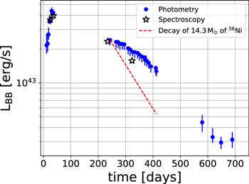
Figure 8. Evolution in time of the bolometric luminosity of a blackbody with the same radiation as PTF 12glz. The star symbols indicate the fits to the spectroscopic data. The dashed line shows the variation in luminosity caused by 14.3 M⊙ of 56Ni radioactively decaying to 56Co and then to 56Fe. LBB decays ≈2 times slower, which suggests that radioactive decay is not sufficient to explain the decay of the light curve and that interaction or other sources of radiation play a role.
Download figure:
Standard image High-resolution imageWe fitted the light curve during the rise time with a function of the form

(where t0 is the time of zero flux, Lmax is the maximum bolometric luminosity, and tc is the characteristic rise time of the bolometric light curve). This allowed us to estimate the epoch at which the extrapolated light curve is crossing zero, which is used throughout this paper as the reference time t0 (MJD) = 56097.58.
As shown in Figure 8, LBB decreases about twice as slowly as the 0.98 mag/100 d decline rate characteristic of the radioactive decay of 56Ni to 56Co and then to 56Fe. If this decline was produced by the radioactive decay of 56Ni, a nickel mass of at least  would be required to reach the bolometric luminosity of PTF 12glz (see Figure 8). The evolution of L should be taken cautiously, because at late time, a blackbody model for the SED may not be valid anymore, and so the temperatures and radii used to calculate L are less reliable. Although the late spectra analyzed in Section 3.1 suggest that the ejecta may have emerged through the CSM at late times, the slow decline of LBB hints at the fact that interaction may still play an important role in the radiation budget (this may happen through radiation from the reverse shock, or through processed radiation through the edge of the wind, or if the ejecta has only partially emerged through the CSM and is still interacting with it in some places).
3.5. Mass of the CSM
A very crude estimation of the swept-up CSM mass can be obtained by assuming that the ejecta mass is comparable to the mass of the CSM and that the bolometric luminosity L is accounted for by the conversion of the kinetic energy of the ejecta into radiation:

where MCSM is the mass of the CSM and ve is the velocity of the ejecta. To an order of magnitude, this estimate will not be very different than estimates based on more realistic treatment of the hydrodynamics (e.g., Ofek et al. 2014a). We use the width FWHM ≈ 8000 km s−1 of the broad Hα component at late time (see Section 3.1) as an approximation of the ejecta velocity ve. From the measured bolometric luminosity shown in Figure 8,  erg. Substituting this value in Equation (2) gives MCSM ≳ 2 M⊙.
In interacting SNe, the optically thick CSM masks the explosion, which may leave an ambiguity about the underlying explosion type. In particular, SNe Ia and core-collapse SNe exploding inside a thick CSM would result in similar observational signatures. The spectra would look similar at early times (as long as the explosion is masked by the CSM) and at very late times, when Ni has decayed and there is no more energy to illuminate the ejecta and create absorption lines in the spectrum. Here, the high value of the bolometric luminosity excludes the possibility that PTF 12glz is a masked SN Ia.
Another order of magnitude estimate of the mass can be obtained by assuming a wind density profile,  and using the photon diffusion timescale (e.g., Ofek et al. 2010),

where κ is the CSM opacity. We assume td ∼ tc, where tc is the characteristic rise time of the bolometric light curve. We estimate tc by fitting the rising part of the bolometric light curve with the exponential function defined in Equation (1) and assuming κ ≈ 0.34 cm2 g−1. We obtain tc ∼ 20 day, and K ≈ 1.5 × 10¹⁷ g cm−1, which corresponds to high values of the density  (or a particle density of n ∼ 1010 cm−3, assuming a mean number of nucleons per particle
  ) at the radii shown in Figure 7.
Measuring K allows us to estimate the mass of the CSM swept up by the ejecta, MCSM(r) ∼ 4πKr (assuming that the CSM extends on much higher scales than the stellar radius). Using the highest early-time radius rBB, shown in Figure 7, as a lower limit of the maximum size of the shell of CSM surrounding the explosion, gives MCSM ≳ 3 M⊙, in good agreement with the estimates obtained with Equation (2).
For a wind density profile,  , where vw is the velocity of the CSM. Therefore, measuring K also gives us an estimation of the mass-loss rate. Using the width of the narrow Hα component during rise time, FWHM ≈ 200 km s−1, as a proxi of vw (see Table 4), we obtain a large mass-loss rate
  ∼ 0.6 M⊙ yr−1, higher than the mass-loss rates observed in Taddia et al. (2013) and Kiewe et al. (2012) and comparable to the mass-loss rate of, e.g., iPTF13z (Nyholm et al. 2017). Combining these estimates suggests that the CSM mass was ejected on a timescale of 1–10 years prior to the SN explosion.
We wish to emphasize that we made several simplifying assumptions in this section. In particular, (1) we assumed a spherical symmetry of the CSM, (2) we assumed a wind profile of the CSM, and (3) we assumed that the kinetic energy of the ejecta converts efficiently into radiation. Therefore, the numbers above have to be considered as order of magnitude estimates.
3.6. Dust Formation?
At late times, the broad component of the Hα Balmer line is blueshifted by ≈1000 km s−1 relative to the galaxy rest frame. The intermediate component is also blueshifted, but by a velocity of ≈250 km s−1, which is consistent with a typical stellar velocity within the galaxy (see Table 4 and Figure 5). Several explanations have been proposed to explain the blueshift of emission line profiles in interacting SN. One possible explanation is the formation of dust, which increasingly blocks the receding parts of the ejecta (e.g., as proposed in the case of the Type IIn SN 2010 jl, Smith et al. 2012; Gall et al. 2014). In our case, the blueshift of the broad component does not grow with time (see Table 4), meaning that if there is dust, it may have formed before the epoch of the first nebular spectrum. In our case, testing the wavelength dependency of the blueshift—a blueshift caused by dust would be stronger at bluer wavelengths—is tricky because the blended iron emission lines mask the structure of the Hβ line profile. We tried to apply several filters on this area, to separate the possible broad Balmer components from Fe ii blend structures, but the results remained inconclusive.
Other explanations have been proposed for the blueshift of emission lines. Fransson et al. (2014), for example, attributed the blueshift of emission lines to radiative acceleration of the preshock gas by the SN radiation, whereas Smith et al. (2012) proposed a geometric explanation.
4. Radiative Diffusion through a Slab
The radiation from an SN exploding into a spherically symmetric CSM has been studied analytically, under simplifying assumptions (e.g., Chevalier 1982; Balberg & Loeb 2011; Ginzburg & Balberg 2014) and numerically (e.g., Falk & Arnett 1977; Moriya & Maeda 2014). The case of an aspherical CSM has been explored to a lesser extent (van Marle et al. 2010; McDowell et al. 2018). Exploring the expected effect of deviation from spherically symmetric CSM on the observables is all the more important because aspherical clouds of CSM around mass-ejecting stars seem to be common, e.g., in stars like η-Carinae (Davidson & Humphreys 1997) that have been proposed as SNe IIn progenitors (e.g., Gal-Yam et al. 2007; Gal-Yam & Leonard 2009). In this section, we attempt to determine whether a nonspherical geometry of the CSM around an SN can explain the growing radius and decreasing temperature observed in Section 3.3. Solving for the exact shape of the CSM from a few observables in an ill-conditioned problem. Therefore, here our goal is merely to verify that a nonspherical geometry can explain the evolution of the observables. Given this goal, we consider a simple aspherical structure: a three-dimensional slab, infinite in two-dimensions and perpendicular to the line of sight.
4.1. Model and Assumptions
We have written a three-dimensional computer program in python, SLAB-Diffusion, available online (Soumagnac 2018, Codebase: https://github.com/maayane/SLAB-Diffusion), in order to calculate the propagation of photons through a slab and simulate the main observables. The simple geometry we consider is illustrated in a cartoon in Figure 9. Following a similar approach as in Ginzburg & Balberg (2014), we replaced the hydrodynamical description of the SN explosion by a stationary model of the shock breakout. This is equivalent to neglecting the expansion of the gas due to the explosion and modeling the interaction between the shock and the CSM as an instantaneous deposition of energy in the slab.
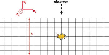
Figure 9. Sketch of the grid used to simulate radiative diffusion through a slab. The dimensions of the slab along the ex and ey coordinates are much larger than h, the dimension of the slab parallel to the line of sight. The initial energy of the explosion is deposited at z = 0, at a distance h/2 from the edge of the slab.
Download figure:
Standard image High-resolution imageThe assumption of an instantaneous release of energy is justified when td/te ≫ 1, where te is the timescale over which the energy of the ejecta is converted into radiation by deceleration, and td is the photon diffusion timescale Equation (3). The timescale te is given by

where Rc is the radius at which the accumulated CSM mass is comparable to the ejecta mass and v is the ejecta velocity. Since td/te = τv/c, the condition td/te ≫ 1 is satisfied, and the instantaneous energy deposition approximation is valid, as long as τ ≫ c/v ∼ 30. This is indeed the case for the model parameters we infer for PTF 12glz: a wind velocity v = 200 km s−1 (Section 3.1) with a mass-loss rate  ∼ 0.6 M⊙ yr−1 (Section 3.5), yielding
  cm and τ ∼ 200.
We assumed that the problem can be treated accurately within the diffusion approximation (i.e., assuming that τ ≈ 1 occurs close to the surface). Hence, the energy density u within the slab is described by the diffusion equation:

where D = c/(3κρ) is the diffusion coefficient. Here we explored three density profiles: a constant density profile, ρ, and two functions of the  coordinate:
  and ρ ∝ z−2, where the origin of the z-axis is at the center of the slab. We leave the treatment of the angular dependency of D to further extensions of this work.
At the boundaries, the energy escapes from the slab and the flux  is linked to the density of energy through

where α ≈ 1/4 (the case α = 1/4 corresponds to isotropic radiation). We discretized Equation (5) in a Cartesian, three-dimensional grid (illustrated in a cartoon in Figure 9), using an explicit forward Euler scheme with ΔtD/(Δd)2 < 0.1 where Δd is defined for each coordinate and is the size of the mesh in each direction  ,
,  , and
, and  . We assumed that D does not depend on the wavelength of the photons (i.e., we made the so-called gray approximation). We solved a dimensionless version of Equation (5):

where t' = tD(h)/h2 and D'(z) = D(z)/D(h). In this case the boundary conditions are

where vd = D(h)/h. A slab with a width h = 1016 cm, an opacity κ = 0.34 cm2 g−1, and a constant mass density ρ = 1 × 10⁻¹⁶ g cm−3 (corresponding, e.g., to 3 M⊙ of CSM in a slab with Lx = Ly = 8 h), corresponds to the unitless velocity v ≈ 1 and a diffusion time td = h23κρ/c = 94 days.
In order to minimize the effect of the finite size of the grid along  and
and  , we took several precautions. We chose the dimensions of the grid along the
  and
and  directions so that Lx = Ly and Lx ≫ h. We checked that Lx is large enough compared to h so that a change in Lx does not affect the results. Equation (8) only describes the boundary conditions along the
  direction. We checked that we can apply reflective boundary conditions (i.e.,
  at the boundaries) or absorbing boundary conditions (i.e., u = 0 at the boundary) along the
  and
and  directions, without affecting the results. We also checked for convergence of the code with respect to the time steps.
4.2. Results
As photons diffuse in the slab, they reach the z = h/2 surface visible to the observer (see Figure 9). In Figure 10, we show the evolution of the total flux of energy escaping from the surface of a slab with v = 1, in response to an instantaneous deposition of energy at t = 0. We use the full width at half maximum (FWHM) of the energy density u at the surface of the slab as a proxy for the radius seen by the observer (below we present another proxy for rBB). In Figure 11, we show that the FWHM grows in time for all three checked density profiles ρ = Const.,  and ρ ∝ z−2. We checked that varying the parameter v does not change this qualitative result.
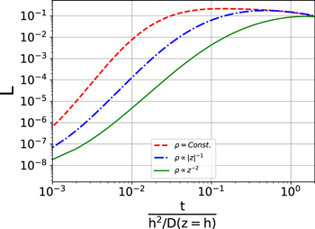
Figure 10. Luminosity  released at the surface of a slab with v = 1, normalized so that the initial energy in the slab is 1. The luminosity is shown for a slab with a constant density profile (dashed line), a density profile
  (dotted line), and a wind density profile ρ ∝ z−2 (continuous line).
Download figure:
Standard image High-resolution image
Figure 11. Full width at half maximum (FWHM) of the density of energy u at the surface of a slab with v = 1. The FWHM is used as a proxy for the blackbody radius measured by the observer. The FWHM is shown for a slab with a constant density profile (dashed line), a density profile  (dotted line) and a wind density profile ρ ∝ z−2 (continuous line).
Download figure:
Standard image High-resolution imageWe would like to check whether our model can reproduce the decrease of the blackbody temperature TBB observed in Figure 7, in addition to producing a growing radius. Here again, given the simplicity of our model geometry, we are interested in the evolution of TBB rather than trying to fit its actual values. By modeling each cell of the z = h/2 surface as a blackbody with temperature T ∝ u(x, y)1/4 and summing up all the cell spectra, we can compute the overall spectrum of the surface. The resultant spectrum is well represented by a blackbody spectrum, which allows us to deduce the blackbody temperature of the surface. This strategy also provides an additional way to recover the growing radius, by using:

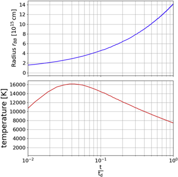
In Figure 12, we show the evolution of the temperature TBB and radius rBB, assuming h = 1 × 1015 cm, a constant mass density ρ = 3 × 10⁻¹⁴ g cm−3 and an input energy of 1051 erg. Using this energy (calculated in Equation (2)) as the energy initially deposited in the slab, is equivalent to assuming that all the energy radiated by the SN explosion is released by the time it starts diffusing out through the CSM. This is only correct within the assumption that the characteristic timescale for diffusion is much larger than the characteristic timescale for interaction between the ejecta and the CSM, which we showed is a correct assumption in the case of PTF 12glz. Figure 12 shows that the aspherical geometry of the slab allows us to recover the increase of the radius rBB and the decrease of the temperature TBB observed in Figure 7.
Figure 12. Evolution in time of: (1) the blackbody radius rBB (top panel) and (2) the blackbody temperature (lower panel) at the surface of a slab with constant density. The diffusion equation was solved with an input energy Ei = 1051 erg deposited in a slab of width h = 1016 cm and a constant mass density ρ = 1 × 10⁻¹⁶ g cm−3, corresponding to td = h23κρ/c = 94 days. The spectrum of the z = h/2 surface was deduced by summing the blackbody spectra of all the cells of the surface and TBB was then deduced by fitting a blackbody to the resultant spectrum. The blackbody radius rBB was deduced through the relation  . The aspherical geometry of the slab allows us to recover the increase of rBB and the decrease in TBB.
Download figure:
Standard image High-resolution image
5. Conclusions
We presented the observations of the supernova PTF 12glz by the GALEX space telescope and ground-based PTF. Radioactive decay is not sufficient to explain the decay of the light curve of PTF 12glz and therefore other physical mechanisms must be involved. One possible—yet difficult to verify—scenario is that an internal engine powers the light curve. Another possible scenario—the standard explanation invoked in the case of SNe IIn, is that the light curve is powered by interaction between the ejecta and the CSM surrounding the SN.
In the case of PTF 12glz, the spectroscopic analysis is consistent with the following picture: at early times (two first spectra) both the ejecta and the shock are initially masked by a thick, slowly moving, photoionized CSM. At later times (two last spectra), the ejecta have emerged through—at least some of—the optically thick layers and have reached CSM layers that are optically thin enough to expose the ejecta. CSM interaction may still play a role at late times, e.g., by heating the ejecta from the inside, and contributes to slowing the light-curve decay.
The evolution of rBB—the radius of the deepest transparent emitting layer—seems to contradict this picture. At early times, i.e., at the very time when the opaque CSM seemingly obstructs our view of any growing structure, rBB grows by an order of magnitude, at a speed of ∼8000 km s−1. In addition to being inconsistent with the spectroscopic analysis, this is also in contradiction—to our knowledge—with all previous observations of either a constant or stalling blackbody radius in SNe IIn (as detailed in Section 3.3).
If the bulk of the radiation from PTF 12glz does come from interaction, the explanation for the growing blackbody radius may be geometrical. The question then is whether any peculiar structure of the CSM around the progenitor can reproduce the observations. In this work, we considered a simple aspherical structure of CSM: a slab. We modeled the radiation from an explosion embedded in a slab of CSM by numerically solving the radiative diffusion equation in a slab with different density profiles: ρ = Const.,  and a wind density profile ρ ∝ z−2. Although this model is simplistic, it allows recovery of the peculiar growth of the blackbody radius rBB observed in the case of PTF 12glz, as well as the decrease of its blackbody temperature TBB. This configuration is not a unique geometrical solution and additional observations, e.g., of the polarization around PTF 12glz would have been necessary to make it less speculative.
As new wide-field transient surveys such as the Zwicky Transient Facility (e.g., Bellm et al. 2015; Laher 2018) are deployed, many more interacting SNe will be observed and quickly followed up with multiple-band observations. These may also be the brightest sources for the ULTRASAT UV satellite mission (Sagiv et al. 2014). Some of these interacting SNe may exhibit the same peculiarities as PTF 12glz. The methodology proposed in this paper offers a framework to analyze them. It could be elaborated upon, to model more complex aspherical geometries, e.g., η Carinae-like shapes of the CSM, and give more quantitative predictions of the observables.
M.T.S. thanks Jonathan Morag, Adam Rubin, Yi Yang, Doron Kushnir, Anders Nyholm, and Chalsea Harris for useful discussions. M.T.S. acknowledges support by a grant from IMOS/ISA, the Ilan Ramon fellowship from the Israel Ministry of Science and Technology and the Benoziyo center for Astrophysics at the Weizmann Institute of Science.
E.O.O. is grateful for the support by grants from the Israel Science Foundation, Minerva, Israeli Ministry of Science, the US-Israel Binational Science Foundation, the Weizmann Institute and the I-CORE Program of the Planning and Budgeting Committee and the Israel Science Foundation.
A.G.-Y. is supported by the EU via ERC grant No. 725161, the Quantum Universe I-Core program, the ISF, the BSF Transformative program, IMOS via ISA and by a Kimmel award.
This work is partly based on tools and data products produced by GAZPAR (https://gazpar.lam.fr) operated by CeSAM-LAM and IAP.
Footnotes
- 13
Sloan Digital Sky Survey; York et al. (2000).
- 14
- 15
MATLAB Astronomy & Astrophysics Toolbox, https://webhome.weizmann.ac.il/home/eofek/matlab/.
- 16
- 17
- 18
- 19