


Abstract
We present optical light curves, redshifts, and classifications for  spectroscopically confirmed Type Ia supernovae (SNe Ia) discovered by the Pan-STARRS1 (PS1) Medium Deep Survey. We detail improvements to the PS1 SN photometry, astrometry, and calibration that reduce the systematic uncertainties in the PS1 SN Ia distances. We combine the subset of
  PS1 SNe Ia (0.03 < z < 0.68) with useful distance estimates of SNe Ia from the Sloan Digital Sky Survey (SDSS), SNLS, and various low-z and Hubble Space Telescope samples to form the largest combined sample of SNe Ia, consisting of a total of
  SNe Ia in the range of 0.01 < z < 2.3, which we call the "Pantheon Sample." When combining Planck 2015 cosmic microwave background (CMB) measurements with the Pantheon SN sample, we find
  and
and  for the wCDM model. When the SN and CMB constraints are combined with constraints from BAO and local H0 measurements, the analysis yields the most precise measurement of dark energy to date:
  and
and  for the
  CDM model. Tension with a cosmological constant previously seen in an analysis of PS1 and low-z SNe has diminished after an increase of 2× in the statistics of the PS1 sample, improved calibration and photometry, and stricter light-curve quality cuts. We find that the systematic uncertainties in our measurements of dark energy are almost as large as the statistical uncertainties, primarily due to limitations of modeling the low-redshift sample. This must be addressed for future progress in using SNe Ia to measure dark energy.
Export citation and abstract BibTeX RIS
1. Introduction
Combining measurements of Type Ia supernova (SN Ia) distances (Riess et al. 1998; Perlmutter et al. 1999) with measurements of the baryon acoustic peak in the large-scale correlation function of galaxies (e.g., Eisenstein et al. 2005; Anderson et al. 2014) and the power spectrum of fluctuations in the cosmic microwave background (CMB; e.g., Bennett et al. 2003; Planck Collaboration et al. 2016a) indicates that our universe is flat, accelerating, and primarily composed of baryons, dark matter, and dark energy. Together, this evidence points to a "standard model of cosmology," yet an understanding of the nature of dark energy remains elusive. Due to improved determinations of cosmological distances, it is now possible to precisely constrain, to better than 10%, the equation of state of dark energy, characterized by the parameter  , where p is its pressure and ρ is its energy density. Furthermore, new measurements (e.g., Betoule et al. 2014, hereafter B14) have begun to place constraints on the evolution of the equation of state with redshift (e.g., with
  ). However, some recent combinations of cosmological probes (e.g., Planck Collaboration et al. 2016a; Riess et al. 2016) do not appear to be consistent with the
  model. To help understand this tension and make a direct measurement of w, SN analyses must both build up the statistics of their samples and examine in greater detail the nature of their systematics.
The leverage on cosmological constraints from SN samples stems from the combination of low-redshift SNe with high-redshift SNe. Over the past 20 yr, there have been a number of SN surveys that together probe a large range in redshift. Many groups have worked on assembling large sets of low-redshift (0.01 < z < 0.1) SNe (e.g., CfA1-CfA4, Riess et al. 1999; Jha et al. 2006; Hicken et al. 2009a, 2009b, 2012; CSP, Contreras et al. 2010; Folatelli et al. 2010; Stritzinger et al. 2011; LOSS, Ganeshalingam et al. 2013). There have been four main surveys probing the z > 0.1 redshift range: ESSENCE (Miknaitis et al. 2007; Wood-Vasey et al. 2007; Narayan et al. 2016), SNLS (Conley et al. 2011; Sullivan et al. 2011), the Sloan Digital Sky Survey (SDSS; Frieman et al. 2008; Kessler et al. 2009a; Sako et al. 2014), and PS1 (Rest et al. 2014; Scolnic et al. 2014a). These surveys have overlapping redshift ranges of 0.1 ≲ z ≲ 0.4 for SDSS, 0.2 ≲ z ≲ 0.7 for ESSENCE, 0.03 ≲ z ≲ 0.68 for PS1, and 0.3 ≲ z ≲ 1.1 for SNLS. Furthermore, there are now high-z data (z > 1.0) from the SCP survey (Suzuki et al. 2012) and both the GOODS (Riess et al. 2004, 2007) and CANDELS/CLASH surveys (Graur et al. 2014; Rodney et al. 2014; Riess et al. 2018). These surveys extend the Hubble diagram out to z = 2.26, from a dark-energy-dominated universe to a dark-matter-dominated universe.
In this paper, we present the full set of spectroscopically confirmed PS1 SNe Ia and combine this sample with spectroscopically confirmed SNe Ia from CfA1-4, CSP, PS1, SDSS, SNLS, and Hubble Space Telescope (HST) SN surveys. The samples included in this analysis are ones that have been cross-calibrated with PS1 in Scolnic et al. (2015, hereafter S15) or have data from HST. While there have been many analyses that combine multiple SN Ia samples, this analysis reduces calibration systematics substantially by cross-calibrating all of the SN samples used (S15). In Betoule et al. (2014), a cross-calibration of SDSS and SNLS (Betoule et al. 2013) was used, but none of the other samples were cross-calibrated. This is particularly important because calibration has been the dominant systematic uncertainty in all recent SN Ia cosmology analyses (B14).
The statistical and systematic uncertainties in recent SN Ia cosmology analyses have been roughly equal. The growing size of the sample has motivated more focus on the systematic uncertainties and also allowed for an examination of various subsamples of the SN Ia population. These tests include probing relations between luminosity and properties of the host galaxies of the SNe (e.g., Kelly et al. 2010; Lampeitl et al. 2010; Sullivan et al. 2010) and analyses of the light-curve fit parameters of SNe and how these parameters relate to luminosity (e.g., Mandel et al. 2017; Scolnic & Kessler 2016). Many of the associated systematic uncertainties of these effects are on the 1% level, and considering that a typical SN distance modulus is measured with roughly 15% precision, it is difficult to properly analyze these effects without SN samples in the hundreds.
This analysis relies heavily on the work by Rest et al. (2014) and Scolnic et al. (2014a), hereafter R14 and S14, respectively. R14 and S14 analyzed the first 1.5 yr of PS1 SN Ia data and combined it with a compilation of low-z surveys. R14 and S14 chose not to analyze any of the higher-z surveys (SDSS, SNLS, HST) so as to focus on the PS1 data sample. Almost every facet of those papers is improved in this analysis. For one important example, the PS1 collaboration recently released photometry of all detected stellar sources (Chambers et al. 2016; Flewelling et al. 2016; Magnier et al. 2016a, 2016b, 2016c; Waters et al. 2016) with subpercent-level relative calibration across 3π sr of the sky; the photometry and calibration of our present analysis are ensured to be consistent with that of the public release.
The SNe Ia presented in this paper include all SNe discovered during the PS1 survey (2009 September–2014 January) that have been spectroscopically confirmed as SNe Ia. The SNe Ia presented in R14 make up roughly 40% of the SNe Ia presented in this paper. Our sample does not include likely SNe Ia in the PS1 sample without spectroscopic classifications. The first effort to analyze these photometric-only SNe was presented in Jones et al. (2017), which is used to improve the PS1 survey simulations in this work. Furthermore, a follow-up analysis of Jones et al. (2017) that determines the cosmological parameters from the full PS1 photometric-only SN sample of ∼1200 SNe (Jones et al. 2018) is a companion analysis to ours and uses multiple pieces of our analysis.
With the set of spectroscopically confirmed SNe Ia discovered by PS1 and multiple other subsamples, we analyze the combined sample to determine cosmological parameters. Due to the number of steps and samples in the analysis, we show Figure 1 to demonstrate the analysis steps. The paper is organized as follows. In Section 2, we present improvements to the PS1 search, photometry, and calibration pipelines. In Section 3, we estimate distances from the PS1 SN sample and discuss simulations of the light curves. In Section 4, we combine the PS1 sample with other samples. In Sections 5 and 6, the full assessment of systematic uncertainties and constraints on cosmology are given. In Sections 7 and 8, we present our discussions and conclusions.

Figure 1. An overview of the various analysis steps in this paper. A common set of steps is done for both the PS1 sample and the combined Pantheon sample.
Download figure:
Standard image High-resolution image2. The PS1 Search, Photometry, and Calibration Pipeline
2.1. Overview of the PS1 Survey
The PS1 data presented here are from the PS1 Medium Deep (MD) Survey, which observes SNe in gri with an average cadence of 7 days per filter.22
This cadence provides well-sampled, multiband light curves. The description of the PS1 survey is given in Kaiser et al. (2010). The PS1 Image Processing Pipeline system (Magnier et al. 2013) performs flat-fielding on each individual image and determines an initial astrometric solution. The full description of these algorithms is given in Chambers et al. (2016), Magnier et al. (2016a, 2016b, 2016c), Flewelling et al. (2016), and Waters et al. (2016). Once done, images are processed in Photpipe (Rest et al. 2005) with updated methodology given in R14.
with an average cadence of 7 days per filter.22
This cadence provides well-sampled, multiband light curves. The description of the PS1 survey is given in Kaiser et al. (2010). The PS1 Image Processing Pipeline system (Magnier et al. 2013) performs flat-fielding on each individual image and determines an initial astrometric solution. The full description of these algorithms is given in Chambers et al. (2016), Magnier et al. (2016a, 2016b, 2016c), Flewelling et al. (2016), and Waters et al. (2016). Once done, images are processed in Photpipe (Rest et al. 2005) with updated methodology given in R14.
The discovery pipeline is explained in R14. The main difference between the pipeline in the first and second half of the survey is that, as the survey went along, the average nightly seeing improved by 0 12 (due to camera/operation improvements) and better templates (>0.5 mag deeper) were used for the transient search. The improved templates also had better artifact removal, which significantly reduced the number of false positives in the transient candidate lists.
The spectroscopic selection over the full survey is similar to that outlined in R14. Spectroscopic observations of PS1 targets were obtained with a variety of instruments: the Blue Channel Spectrograph (Schmidt et al. 1989) and Hectospec (Fabricant et al. 2005) on the 6.5 m MMT, the Gemini Multi-Object Spectrographs (GMOS; Hook et al. 2004) on both Gemini North and South, the Low Dispersion Survey Spectrograph-3 (LDSS323 ) and the Magellan Echellette (MagE; Marshall et al. 2008) on the 6.5 m Magellan Clay telescope, the Inamori-Magellan Areal Camera and Spectrograph (IMACS; Dressler et al. 2011) on the 6.5 m Magellan Baade telescope, the ISIS spectrograph on the WHT,24 and DEIMOS (Faber et al. 2003) on the 10 m Keck telescope.
Since there were a multitude of spectroscopic programs without a well-defined algorithm to determine which candidates to observe, an empirical algorithm is retroactively determined that best describes our selection of spectroscopic targets. This is discussed further in Section 3, but we note here that the spectroscopic selection for the full survey is very similar to that of the first 1.5 yr of the PS1 survey described in R14. The one exception was a program by PI Kirshner (GO-13046) to observe HST candidates for infrared follow-up specifically at z ∼ 0.3. A table of the spectroscopically confirmed SNe Ia that includes the dates of the observations and the telescopes used is given in Appendix A.
The distribution of redshifts of the confirmed SNe Ia is shown in Figure 2. The median redshift is 0.3, which is Δz ∼ 0.05 smaller than the median redshift of likely photometric SNe Ia discovered during the survey (Jones et al. 2017). As shown in Figure 2, the observed candidates are well dispersed over the focal plane with no systematic grouping at one focal position. It is also shown in Figure 2 that the majority of candidates are discovered before peak. A discovery (defined as three detections with signal-to-noise ratio (S/N) > 4) after peak does not exclude the possibility that there were pre-explosion images acquired, only that the object was not detected at that time.

Figure 2. Histograms comparing the set of all spectroscopically confirmed SNe Ia against the subset that is deemed cosmologically useful. Filled bars indicate the full spectroscopic sample of  SNe Ia, while outlined bars indicate the
  used for our cosmology analysis. Top: distribution of redshift. Middle: distribution of radial angular distance from center of focal plane. Bottom: distribution of the age at discovery as determined from the date of peak brightness subtracted from the discovery date.
Download figure:
Standard image High-resolution image2.2. Improvements to PS1 Photometry
The photometry pipeline used in this analysis is a modified version of that described in R14. The overall process used is summarized as such:
- 1.Template Construction. For each PS1 chip, templates are constructed from stacking multiple, nightly, variance-weighted images from all but a single survey year around the SN explosion date. The seasonal templates are made of ∼60+ images and reach 5σ depths of 25.00, 25.1, 25.15, and 24.80 mag in gri
 . Excluding a particular year removes the possibility that >1 mmag of SN flux is included in the template. We develop a scene-modeling pipeline (e.g., Holtzman et al. 2008) as an independent cross-check on the template construction. This is presented in Appendix B.
 - 2.Astrometric Alignment. All nightly images and templates are astrometrically aligned with an initial catalog provided by the PS1 survey. For all bright stars and galaxies observed on each CCD with an SN observation, an astrometry catalog is recreated with the average locations of each of the stars and galaxies over the full survey. Then an astrometric solution for each nightly image and template is determined to match the improved catalog.
- 3.Stellar Zero-points. Point-spread function (PSF) photometry is performed on the image at the positions of the stars from the final catalog; there is no re-centroiding of the star's position per image, such that "forced" photometry is done. The PSF module is based on a Python implementation (Jones et al. 2015) of the DAOPhot package (Stetson 1987). A comparison of the photometry of these stars to updated PS1 stellar catalogs is used to find the zero-point of each image. Forced photometry on the stars is necessary so that a consistent procedure is done for both the stars and the SNe. The PSF is determined for each epoch from neighboring stars of the SN. Due to the fast-varying PSF on CCDs near the center of the focal plane (<0
 4), the region cutout to find neighboring stars is roughly 1/4 the area of the chip. For CCDs away from the center of the focal plane (>04), the full area of the 12
 5 chip is used.
 - 4.Template Matching. Templates are convolved with a PSF to match the nightly images (Becker 2015). The convolved templates are then subtracted from the nightly images.
- 5.Forced SN Photometry. A flux-weighted centroid is found for each SN position. Forced photometry is performed at the position of the SN. The nightly zero-point is applied to the photometry to determine the brightness of the SN for that epoch. Small adjustments are made to the SN photometry based on the expectation value from the astrometric uncertainty of the SN centroid. Forced photometry is also applied to random positions in the difference image to empirically determine the amount of correlated noise in the image. The SN photometry uncertainties are then increased to account for this correlated noise.
- 6.Flux Adjustment. The errors and the baseline flux of the SN measurements are adjusted so that the mean pre-explosion baseline flux level is 0 and the reduced χ2 is near unity. The prescription for this step is described in R14.

The most significant changes relative to R14 are the additions of iterative astrometric alignment, forced photometry of stars with an updated PSF fitting routine, an updated Ubercal catalog, and a reduction in the area from which neighboring stars are drawn for building PSF models. These steps improve the accuracy of the astrometric solution, alleviate systematic uncertainties in the photometry due to uncertainties in the astrometry, and account for the fast-varying PSF near the center of the focal plane, respectively.
Improvements to understand the systematic uncertainties in this process are discussed below. The systematic uncertainties in the photometry analysis are given in Table 1.
Table 1.
The Dominant Systematic Uncertainties in Defining the Pan-STARRS1 Photometric System. Each of the Numbers given is the Average Over the Four Filters gri . The bandpass uncertainties are 7 Å
| Source | Uncertainty |
|---|---|
| (mmag) | |
| SN Photometry | |
| Astrometric uncertainty | 1 |
| Template construction | 1 |
| Photometric nonlinearity | 2 |
| Internal Calibration | |
| Ubercal zero-points | 1 |
| Spatial variation | 1 |
| Temporal variation | 1 |
| Focal plane variation | 2 |
Download table as: ASCIITypeset image
2.2.1. Astrometry
The recovered position of an SN detection can be different from the true SN centroid for the following reasons: accuracy of the WCS for a given image, the limited number of observations of the SN, Poisson noise from sky, host galaxy, and SN and difference image artifacts. Unlike in R14, forced photometry is performed on both stars and SNe, so the errors on SN positions and stellar position are similar and do not propagate to additional biases. However, uncertainties that affect only the SN position are treated separately.
R14 shows that the astrometric uncertainty of objects depends on both the FWHM and S/N of the object. Because of the S/N dependence, the astrometric uncertainty of the higher-redshift SNe is larger than the astrometric uncertainty of the lower-redshift SNe. This astrometric uncertainty will propagate to a photometric bias because the expected average offset from the true centroid value causes biased photometric measurements. To understand this trend, the astrometric uncertainty of the individual detections is quantified. This is done in R14 by first finding the linear relation between astrometric uncertainty (e.g.,  , here denoted as
  ) and
) and  :
:

where the astrometric uncertainty σa in pixels of a given detection has a floor mostly due to pixelization ( ), and in addition a random error σa2. R14 conservatively uses σa1 =0.20 pixels and σa2 = 1.5 to calculate the astrometric uncertainty of a single detection. In Figure 3, it is clear that the quantified relation from R14 is too high by a factor of 2 for our sample owing to our improved astrometry such that we find the uncertainty of astrometry as we find a σa1 = 0.1 and σa2 = 0.75. Much of this improvement is from the iterative astrometric alignment discussed above.

Figure 3. Top: plot of the variance of recovered pixel offsets in one dimension (y) vs. (FWHM/S/N)2. A similar overestimation of the astrometric error by R14 is seen in the x direction as well. Bottom: necessary photometric bias correction vs. redshift of the SN due to the expected astrometric uncertainty of the central position of an SN from the combined series of images of that SN in one filter. A best-fit line is overlaid in yellow.
Download figure:
Standard image High-resolution imageThe relation in Figure 3 is used to determine the astrometric uncertainty of each SN observation to properly determine the centroid accuracy of the SN. With a more appropriate estimate of the astrometric uncertainty, the centroids and centroid errors are recalculated for each SN detection. To remove the expected bias in the photometry from the centroid error, a conversion from R14 is applied between the astrometric uncertainty  and the bias in photometry
  from Equation (1) such that

where PDF(σa, t) is the probability density function with sigma  and pixel variable t, assuming that h is constant and independent of S/N. The value of h (0.043) is taken from R14 and is found to be a reliable first-order approximation. The corrections to the photometry for each SN are shown in the bottom panel of Figure 3. The maximum correction is 6 mmag.
2.3. Improvements to Photometric Calibration
The absolute calibration of the PS1 photometric system has been improved in a series of PS1 analyses. The basis for the PS1 absolute calibration is first presented in Tonry et al. (2012), and a full review of subsequent improvements is given in Scolnic et al. (2015). The relative calibration across the sky of the PS1 survey is determined by the Ubercal process (Schlafly et al. 2012; Finkbeiner et al. 2016). For the MD fields, we made a custom Ubercal star catalog of all of the data from the MD fields in the same way as those produced in Schlafly et al. (2012) but with a higher-resolution nightly flat field, a lower threshold for masking of problematic areas of the focal plane, and a per-image zero-point. These catalogs are released with results from this paper at doi:10.17909/T95Q4X and are consistent with Schlafly et al. (2012) in relative calibration on degree scales to the 1 mmag level. Scolnic et al. (2015), using the same catalogs as in this current analysis, show in comparisons with SDSS and SNLS that the likely systematic uncertainty of the zero-points of each MD field for each filter is ∼3 mmag.
The nightly photometry is transferred onto the PS1 system using a zero-point measured by comparing the photometry with stellar magnitudes from the Ubercal catalog. The result of this process is shown in Figure 4, which presents differences between our PS1 catalogs and the final nightly photometry. As the Ubercal catalogs are used to determine both the calibration of the HST Calspec standards and the MD fields, Figure 4 demonstrates the consistency of the nightly photometry with that used to create the PS1 calibration across 3π of the sky. We find that the nightly photometry and Ubercal catalogs are consistent across 4 mag to levels of ∼2 mmag, though with a trend in the discrepancy of ∼1 mmag per mag as shown with a linear fit overlaid on the left panel of Figure 4. It is unclear what is causing this trend, and it is possible that this small trend is partly due to selection effects in the cuts made to make the catalogs. This trend is therefore included as part of our systematic error budget. Image zero-points for each observation are determined using stars brighter than 21.5, 21.0, 21.0, and 21.0 in  , respectively. Future analyses may try to use an S/N cut instead of a magnitude cut to reduce the Malmquist bias. Possible nonlinearity has been tested in Scolnic et al. (2015) in comparisons of PS1 with SDSS, SNLS, and multiple low-z surveys: using our PS1 stellar catalogs, linearity behaves to better than 3 mmag in gri
 between 15 and 21 mag. Further discussions of PS1 detector nonlinearity are in Waters et al. (2016).

Figure 4. Agreement between g-band nightly photometry and Ubercal photometry of  million stars and the dependence on magnitude, MJD, airmass, and focal plane position. Different colors of the points represent bins of stellar colors. In the right panel, arrows indicate that the R14 discrepancy with the catalog photometry near the center of the focal plane was >0.1 mag.
Download figure:
Standard image High-resolution imageSystematic uncertainties in our photometry, due to spatial variation of the throughput across the focal plane, as well as temporal variation of the filters over the entire survey, are examined here as well. There is no evidence (<1 mmag) of differences in the system photometry over the full course of the survey. There is also excellent agreement (<1 mmag) between the stellar photometry from our pipeline and the Ubercal catalogs across the focal plane. A much larger effect (>0.15 mag) was seen in R14 owing to the fast-varying PSF (change of 1 pixel in FWHM over 04) near the center of the focal plane that was not accounted for. Therefore, in R14, SNe near the center (r < 04) of the focal plane were not used in the analysis. This problem has been fixed by reducing the area for choosing neighboring stars from which to build a PSF near the center of the focal plane. Furthermore, there is little dependence (<2 mmag) on the airmass of the nightly observations.
In S14, the filters used to measure the SN light curves are those given at the median radial position across the field of view. From measuring the expected photometry of synthetic SN spectra integrated through the known PS1 passbands at various focal positions, differences in the photometry of the SN dependent on focal plane position increase scatter by 0.01 mag. However, S14 showed that there is only a 2 mmag bias with redshift due to the different passbands. Further corrections based on the airmass of each observation, as done in Li et al. (2016), may be implemented in the future; however, it is shown in Figure 4 that the impact is on the 1 mmag scale. All uncertainties are summarized in Table 1.
3. PS1 Light-curve Fitting and Simulation
We measured photometry of the total set of  confirmed SNe Ia. In Figure 5, three representative PS1 SN Ia light curves are shown. All light curves are available in machine-readable format at doi:10.17909/T95Q4X.

Figure 5. Representative light curves of SNe from the PS1 survey: PS1-520022, PS1-370394, and PS1-380040 from top to bottom, respectively. These SNe have redshifts of z = 0.12, 0.33, and 0.68. The points shown are data from the PS1 survey, and the curves shown are fits using SALT2. The flux units are given for a zero-point of 27.5 mag in each band.
Download figure:
Standard image High-resolution image3.1. Blinding the Analysis
It is difficult to fully blind an analysis of this sort, since any update in photometry, calibration, etc., of a sample has a direct, and sometimes obvious, impact on recovered cosmological parameters. As discussed later in this section, we use the BEAMS with Bias Corrections (BBC) method (Kessler & Scolnic 2017) to recover binned Hubble residuals with redshift, with respect to a reference cosmology. Therefore, to blind the analysis, the reference cosmology is randomly chosen. So that a full analysis can be completed without introducing any further SN systematics based on a highly unlikely cosmology, the reference cosmology is randomly chosen from a Gaussian distribution of values of the matter density Ωm and equation of state of dark energy w (discussed in Section 5) centered around the recovered values in the B14 analysis of w = −1.02 and Ωm = 0.307 with a standard deviation of σw = 0.06 and  , where the standard deviation is determined from the uncertainties on the cosmological parameters in the B14 analysis. We use the B14 analysis to choose the blinding parameters rather than R14 because the full sample that this paper will analyze is more consistent with that in B14 than that in R14 and has lower uncertainties.
3.2. Light-curve Fitting
While multiple light-curve fitters can be used to determine accurate distances (e.g., Jha et al. 2007; Guy et al. 2010; Burns et al. 2011; Mandel et al. 2011), we use SALT2 (Guy et al. 2010) for this analysis, as it has been trained on the JLA sample (B14) and it is easy to assess various systematic uncertainties with this fitter. We use the most up-to-date published version of SALT2 presented in B14 and implemented in SNANA25 (Kessler et al. 2009b). Differences between the SALT2 spectral model in Guy et al. (2010) and that in B14 are mainly due to calibration errors in the light curves used for the model training. The models differ the most at rest-frame wavelengths <4000 Å and are described in detail in B14. Three values are determined in the light-curve fit that are needed to derive a distance: the color c, the light-curve shape parameter x1 and the log of the overall flux normalization mB. The solid lines in Figure 5 show the respective light-curve fits with SALT2 for three representative PS1 SNe Ia.
The SALT2 light-curve fit parameters are transformed into distances using a modified version of the Tripp formula (Tripp 1998),

where μ is the distance modulus, ΔM is a distance correction based on the host galaxy mass of the SN, and ΔB is a distance correction based on predicted biases from simulations. Furthermore, α is the coefficient of the relation between luminosity and stretch, β is the coefficient of the relation between luminosity and color, and M is the absolute B-band magnitude of a fiducial SN Ia with x1 = 0 and c = 0. Motivated by Schlafly & Finkbeiner (2011) and following S14, we modify SALT2 by replacing the "CCM" (Cardelli et al. 1989) Milky Way (MW) reddening law with that from Fitzpatrick (1999).
The total distance error of each SN is

where  is the photometric error of the SN distance,
  is the distance uncertainty from the mass step correction,
  is the uncertainty from the distance bias correction,
  is the uncertainty from the peculiar velocity uncertainty and redshift measurement uncertainty in quadrature,
  is the uncertainty from stochastic gravitational lensing, and
  is the intrinsic scatter. For this analysis,
  as given in Jönsson et al. (2010).
For this analysis, we require every SN Ia to have adequate light-curve coverage to accurately constrain light-curve fit parameters, as well as properties that limit systematic biases in the recovered distance. We follow the light-curve requirements in B14 such that the only SNe allowed in the sample have −3 < x1 < 3, −0.3 < c < 0.3,  , and σx1 < 1 (where
  is the uncertainty on the rest-frame peak date and
  is the uncertainty on x1). Most of the cuts, as shown in Table 2, are motivated by B14. The cuts are somewhat different than those used in R14 that require observations before and after the peak brightness date. These updated requirements are more stringent than those used in R14, though three of the SNe Ia that do not pass the R14 cuts do pass these new cuts. These three SNe Ia are all at low z, where it was unclear if there were observations taken before peak owing to uncertainty in the peak date, though the i-band peak was measured accurately. A related issue due to uncertainty in the peak date was pointed out in Dai & Wang (2016), which finds ∼10 SNe with double-peak probability distribution functions of the light-curve parameters of the SALT2 fits. We find that many (8/10) of these SNe would be removed from our set if we place an additional cut enforcing observations after post-maximum brightness. Therefore, we include a cut such that there is an observation at least 5 days after peak brightness. B14 also places a requirement for
  . This does not apply to the PS1 SN sample but will apply to other samples, as all the MD fields have low extinction, and as discussed in S14, this constraint is loosened to
  owing to improved nonlinear modeling of high extinction (Schlafly & Finkbeiner 2011). Furthermore, in B14, a cut on the fit likelihood is placed on the SDSS SNe Ia but not on the SNLS sample in B14. We follow the strategy for the SDSS sample and place a cut on the χ2/NDOF < 3.0. Finally, there is one last additional cut from the BBC method that removes three of the SNe because their x1 and c parameters do not fall in the expected distribution—this is discussed in Section 3.5. Applying these cuts, only
  SNe Ia from the initial sample of
  spectroscopically confirmed Pan-STARRS1 objects remain in our sample for a cosmological analysis.
Table 2.
Impact of Various Cuts Used for Cosmology Analysis. Both the Number Removed from Each cut and the Number Remaining After Each Cut are Shown. The "Quality fit" Includes Both the Light Curves that are Rejected by the SNANA Fitter Owing to Poorly Converged fits and those with a fit 
| Discarded | Remaining | |
|---|---|---|
| Initial | ⋯ |

|
| Quality fit |

|

|

|

|

|

|

|

|

|

|

|
| −3 < x1 < 3 |

|

|

|
0 |

|

|

|

|
| BBC cut | 3 |

|
Download table as: ASCIITypeset image
The SALT2 parameters for the entire set of cosmologically useful SNe Ia from the PS1 sample are presented in Appendix A. A table with the full output of each SNANA fit with SALT2 is included at doi:10.17909/T95Q4X.
3.3. Survey Simulations
To correct for biased distance estimates, the PS1 SN survey must be accurately simulated. Following S14, we simulate the PS1 survey with SNANA using cadences, observing conditions, spectroscopic efficiency, etc., from the data. Following Jones et al. (2017), we include a complete library of observations of the PS1 survey, noise contributions from the host galaxies of the SNe Ia, and a newly modeled SN discovery efficiency. The noise contributions from the host galaxies were modeled for the PS1 photometric sample, which is a good approximation for the confirmed sample, as the average host galaxy magnitudes for the confirmed and photometric samples are within 0.1 mag.
To model the spectroscopic selection of the PS1 SN survey, an efficiency function must be empirically determined. Similar to R14, we find that it is well modeled with a dependence on the peak r-band magnitude of the SN. The function is shown in the top panel of Figure 6. The method to determine this function is analogous to the approach taken in Scolnic & Kessler (2016, hereafter SK16) for determining the underlying color populations. We simulate PS1 without a spectroscopic efficiency function and divide the distribution of r magnitudes at the peak of the light curves from the data by that from the simulation. The ratio is the spectroscopic efficiency function, and the final curve shown in Figure 6 is smoothed from the recovered function. A coherent shift of the selection function by 0.25 mag in one direction is found to reduce the match between the predicted and actual redshift distribution by 1σ, and this error is overlaid in Figure 6.

Figure 6. Top: PS1 spectroscopic selection efficiency as a function of peak r-band magnitude. The shaded band denotes the 1σ uncertainty on the function. Bottom: predicted distance bias that is caused from the selection effects using the Tripp estimator from simulations with two different intrinsic scatter models. The average distance bias between the two is also displayed.
Download figure:
Standard image High-resolution image3.4. Populations and Intrinsic Scatter Models
The underlying population of the stretch and color of the PS1 light curves is redetermined for the full data sample according to the process described in SK16. These are given in Table 3 for two different models of the Gaussian intrinsic scatter of SNe Ia: the "C11" model that is composed of 75% chromatic variation and 25% achromatic variation (Chotard et al. 2011), and the "G10" model that is composed of 30% chromatic variation and 70% achromatic variation (Guy et al. 2010). Besides scatter models that have 100% of one type of variation, the C11 and G10 models are the only two published models available for this type of analysis, and either of them may accurately represent the PS1 SN population. To use these models in simulations, Kessler et al. (2013) convert broadband models into spectral variation models. The color population parameters in Table 3 show agreement within 1σ between this analysis and that derived for the PS1 R14 sample (SK16). The stretch population parameters appear to be slightly discrepant, though this difference is exaggerated because we do not report covariances between  ,
,  , and
, and  : the mean of the distribution of recovered x1 values for the full PS1 sample is Δx1 ∼ 0.03 from the mean of the x1 distribution from R14.
Table 3.
Underlying Populations of SN Ia x1 and c Parameters for the Full PS1 Sample and those Found in SK16. The First Column Shows the Analysis, and the Second Column Shows the Scatter Model Used in the Simulation. The First Part of the Table Shows the Recovered Values of the Underlying Color (c) Population, and the Second Part of the Table Shows the Recovered Values of the Underlying Stretch (x1) Distribution. These Parameters Define the Asymmetric Gaussian for the Color and Light-Curve Shape Distributions: ![${e}^{[-{(x-\bar{x})}^{2}/2{\sigma }_{-}^{2}]}$](https://content.cld.iop.org/journals/0004-637X/859/2/101/revision1/apjaab9bbieqn73.gif) for
for  and
and ![${e}^{[-{(x-\bar{x})}^{2}/2{\sigma }_{+}^{2}]}$](https://content.cld.iop.org/journals/0004-637X/859/2/101/revision1/apjaab9bbieqn75.gif) for
for 
| Analysis | Scat. |

|

|

|
|---|---|---|---|---|
| This work | G10 | −0.068 ± 0.023 | 0.034 ± 0.016 | 0.123 ± 0.022 |
| This work | C11 | −0.100 ± 0.004 | 0.003 ± 0.003 | 0.134 ± 0.016 |
| SK16 | G10 | −0.077 ± 0.023 | 0.029 ± 0.016 | 0.121 ± 0.019 |
| SK16 | C11 | −0.103 ± 0.003 | 0.003 ± 0.003 | 0.129 ± 0.014 |

|

|

|
||
| This work | G10 | 0.365 ± 0.208 | 0.963 ± 0.162 | 0.514 ± 0.140 |
| This work | C11 | 0.384 ± 0.200 | 0.987 ± 0.155 | 0.505 ± 0.135 |
| SK16 | G10 | 0.604 ± 0.183 | 1.029 ± 0.138 | 0.363 ± 0.121 |
| SK16 | C11 | 0.589 ± 0.179 | 1.026 ± 0.137 | 0.381 ± 0.117 |
Download table as: ASCIITypeset image
The population parameters given here are derived from simulations that assume a  model. SK16 found that changes in the input cosmology within typical statistical uncertainties have a <0.2σ effect on the recovered populations. R. C. Wolf et al. (2018, in preparation) improves on the analysis of SK16 by attempting to fit for cosmological parameters and these population parameters simultaneously.
Figure 7 shows how well simulations model the data by comparing the distribution of redshift, constraint on time of maximum light, color error, and peak S/N distribution compared to the data. Comparisons of the color and stretch distributions, as well as their trends with redshift, are also shown. There is substantial improvement from S14 in how well the simulations and data match owing to more statistics in our sample and better modeling methods.

Figure 7. Comparison of distributions for PS1 data (points) and simulations (histograms), where each simulation distribution is scaled to have the same sample size as the data. We show the simulation of the survey assuming a G10 scatter model for the intrinsic dispersion (red) and assuming a C11 scatter model (green). The distributions are shown over redshift, error in the peak MJD, error in the color c, peak S/N of the light curve, fitted SALT2 color (c), and light-curve shape parameter (x1). The bottom two panels show the SALT2 color (c) and shape parameter (x1) vs. redshift.
Download figure:
Standard image High-resolution image3.5. BBC Method
SK16 and Kessler & Scolnic (2017, hereafter KS17) show that the Tripp estimator does not account for distance biases due to intrinsic scatter and selection effects. KS17 introduces the BBC method to properly correct these expected biases and simultaneously fit for the α and β parameters from Equation (3). The method relies heavily on Marriner et al. (2011) but includes extensive simulations to correct the SALT2 fit parameters mB, c, and x1. In Equation (1), this correction is expressed as ΔB, which is actually a function of α, β, ΔmB, Δc, and Δx1 that follows the same Tripp format such that  . Furthermore, the measurement uncertainty σN in Equation (2) is similarly corrected according to predictions from simulations because KS17 shows that the fit with SALT2 regularly overestimates the uncertainties of the fit parameters. Finally, the BBC method requires that the properties of an SN in the data sample are well represented in a simulation of 500,000 SNe, so any SNe with z, c, and x1 properties that are not found within 99.999% of the simulated sample will not pass the BBC cut. The impact of the BBC cut is given in Table 2. The three SNe that are cut have x1 and/or c values removed from the distribution as shown in Figure 7. They have (x1, c) values of (−2.915, 0.083), (−1.702, 0.271), and (−0.893, 0.298). A simpler cut would be to shrink the current x1 range from (−3, 3) and the c range of (−0.3, 0.3) to narrower ranges, and this will be studied in the future.
Given accurate simulations of the survey, the BBC method retrieves the nuisance parameters α and β from Equation (3) and derives the distances of each SN. As discussed in KS17, the recovered nuisance parameters depend on assumptions about the intrinsic scatter model. The method returns α =  , β =
, β =  , and σint =
  when assuming the G10 scatter model and
  ,
,  , and
, and  when assuming the C11 scatter model. The difference in σint values is related to the assumed variation in the scatter model; the dispersion of Hubble residuals from both of these fits is about equal at σtot = 0.14 mag.
We can calculate the dependence of the bias in recovered distance on redshift by simulating the survey with both scatter models and measuring the difference between the true and recovered distances. In the bottom panel of Figure 6, we show the distance bias when we simulate the two different scatter models with their associated β values (G10:  C11:
C11:  ), but we assume that the true scatter model was the G10 model (effectively determining distances with β = 3.0). The biases calculated using the two different scatter models are within 5 mmag for almost the entire redshift range until z ∼ 0.6. The uptick at high z is due to the interplay between color and brightness selection and is discussed further in Section 5.
3.6. Comparisons with R14
Figure 8 shows a comparison of the mean distances in redshift bins between the R14 sample and our sample. This is shown for before and after distance bias corrections are applied. For the BBC method, the average of the corrections from the two scatter models is used. Our sample has roughly twice as many SNe as the R14 sample, so the comparisons show both statistical differences and systematic differences between the two samples. Relative to a reference cosmology, one indication of a trend is observed in the R14 sample but not in our sample: an increasing positive distance bias with redshift. This trend appears significant in the R14 sample owing to the highest-z bin, which has a positive residual of ∼0.3 mag. That residual is driven by only two SNe, both with high (>0.25 mag) residuals. In our sample, one of these SNe is cut owing to the selection cuts, and one of them has significantly changed photometry by 0.3 mag owing to low S/N and poor astrometry. Smaller differences are driven by changes in the calibration of both the PS1 system and the SALT2 model.

Figure 8. Hubble residuals of the data to a reference cosmology for R14 and our analysis. The residuals are shown before any distance bias corrections (top) and after distance bias corrections (bottom). The top panel shows differences due to improved statistics, calibration, and photometry. The bottom panel shows further differences due to the improved bias corrections. All bins with >0 SNe are shown, and differences at high z are driven by changes in photometry and different selection cuts. The centers of the redshift bins with the BBC method are re-weighted using the SN distance uncertainties.
Download figure:
Standard image High-resolution image3.7. Mass Determination
Multiple SN Ia analyses (discussed below) show that there is a correlation between luminosity of the SNe and properties of the host galaxies of the SNe Ia. This effect is important for measuring cosmological parameters, as the demographics of SNe with certain host galaxy properties may change with redshift, and also because correcting for the effect may reduce the scatter of the distances. Correlations between luminosity and the host galaxy mass (e.g., Kelly et al. 2010; Lampeitl et al. 2010; Sullivan et al. 2010), age, metallicity, and star formation rate (e.g., Hayden et al. 2013; Roman et al. 2017) have all been shown. So far, the relation with mass appears to be the strongest of the correlations, possibly because it is easier to measure the mass of galaxies than the other properties, so in this analysis we use the mass dependence. In S14, the difference in the mean Hubble residual for SNe in galaxies with high versus low masses (at a split of  ) was found to be 0.037 ± 0.032 mag, which is consistent with a null result, as well as with the B14 statistical result of 0.06 ± 0.012 mag. In this analysis, our statistics are a factor of 2 larger and allow us to better measure the step.
The masses of PS1 host galaxies are derived similarly to S14 and follow the approach in Pan et al. (2014). Here we use the seasonal templates, discussed in Section 2, to measure host galaxy photometry, and we combine PS1 observations with u-band data from SDSS (Alam et al. 2015) where available. SExtractor's FLUX_AUTO (Bertin & Arnouts 1996) was used to determine the flux values in  ,
,  ,
,  ,
,  ,
,  . The measured magnitudes are analyzed with the photometric redshift code Z-PEG (Le Borgne & Rocca-Volmerange 2002), which is based on the PEGASE.2 spectral synthesis code (Fioc & Rocca-Volmerange 1999) and follows da Cunha et al. (2012) to calculate the stellar masses of host galaxies. This is a very similar analysis code to what is used to determine the masses of the host galaxies in the JLA sample (B14). Further details of the assumptions used to run the code are discussed in Pan et al. (2014).
Masses are determined by the Z-PEG code for all but four of the  PS1 host galaxies. For the four SNe without matched host galaxies, no host galaxy was detected near the SN. The masses of the hosts of these SNe are placed in the lowest mass bin (as done in B14). The mass step is typically placed at 1010 M⊙, and we find that there are
  host galaxies with masses higher than the split value and
  with masses lower than the split value. In Figure 9, we show relations between the stretch, color, and Hubble residuals of the SNe Ia with the mass of the host galaxies. We find no trend with color such that the mean color of SNe in low-mass hosts is −0.001 ± 0.004 mag smaller than the color for SNe with high-mass hosts. We also recover the typical trend such that SNe with lower stretch values are more often found in high-mass hosts, with a median difference in stretch values between high- and low-mass hosts of Δx1 = 0.210 ± 0.041.

Figure 9. Correlations in the data between color, stretch, and Hubble residuals with host galaxy mass. A vertical line is shown at a host galaxy mass equal to  . Steps are expressed as parameters for the higher-mass group minus the lower-mass group.
Download figure:
Standard image High-resolution imageThe split in luminosity with mass is determined by three parameters: a relative offset in luminosity, a mass step for the split, and an exponential transition term in a Fermi function that describes the relative probability of masses being on one side or the other of the split:

The Fermi function that is chosen here is used to allow for both uncertainty in the mass step and uncertainty in the host masses themselves. For the PS1 sample,  mag, mstep = 10.02 ± 0.06, and τ = 0.134 ± 0.05. The step
  is similar to that found in S14, although with a smaller uncertainty. Interestingly, if we did not apply the BBC method, as done in S14, we find for this sample
  mag. This is roughly 1σ larger than with the BBC method and is more consistent with the mass step recovered in B14 of 0.06 ± 0.012 mag, which also did not implement the BBC method.
To test how the BBC method accounts for a relation between mass and luminosity, we created new simulations with host galaxy mass properties assigned to every SN. We assigned a host mass to each SN so that the simulated sample replicates the trends of mass with c and x1 seen in Figure 9. Applying Equation (5) to the simulations using the BBC method, we see a bias of only 0.0035 mag in the recovered value of γ given an input value of γ = 0.08 mag. Furthermore, we find that including a mass step has only a 0.001 mag effect on the distance bias corrections shown in Figure 6 and therefore has a limited impact on our analysis.
4. Combining Multiple SN Samples
The PS1 survey is the latest in a long line of programs designed to build up a set of cosmologically useful SNe Ia. To optimally constrain the cosmological parameters, we supplement the PS1 data with available SN Ia samples: CfA1–CfA4 (Riess et al. 1999; Jha et al. 2006; Hicken et al. 2009a, 2009b, 2012), CSP (Contreras et al. 2010; Folatelli et al. 2010; Stritzinger et al. 2011), SNLS (Conley et al. 2011; Sullivan et al. 2011), SDSS (Frieman et al. 2008; Kessler et al. 2009a), and high-z data (z > 1.0) from the SCP survey (Suzuki et al. 2012), GOODS (Riess et al. 2007), and CANDELS/CLASH survey (Graur et al. 2014; Rodney et al. 2014; Riess et al. 2018). We do not include samples like Calan Tololo that were not in Scolnic et al. (2015), and following Scolnic et al. (2015), we separate CfA3 into two subsurveys CfA3K and CfA3S and CfA4 into two periods CfA4p1 and CfA4p2. These surveys extend the Hubble diagram from z ∼ 0.01 out to z ∼ 2. We note that because of the difficulty of high-z spectroscopic identification, the confidence in the spectroscopic identification of the z > 1 HST SNe is not quite as high as for the z < 1 SNe, but this is addressed in each of the papers above, and we only include SNe that are at a "Gold"-like level. In total, there are  SNe that are used in our cosmology analysis, and we refer to this sample as the "Pantheon sample." The numbers of SNe from each subsample that are used in our cosmology analysis are shown in Table 4. The differences in the number of low-z SNe that pass the cuts compared to R14 (given in number of SNe from R14 minus number of SNe from our Pantheon sample) are as follows: CSP (
 ), CfA1 (
 ), CfA2 (
 ), CfA3 (
 ), CfA4 (
 ). The largest difference here is from CSP, which may have underestimated their photometric error uncertainties so that the
  values returned are typically too high to pass the quality cut. This is briefly discussed in Appendix C.
Table 4. Total Numbers of SNe Ia From Surveys Included in the Pantheon Sample after All Sample Selection Cuts for Cosmological Analysis are Applied, as well as the Mean Redshift of Each Subsample
| Sample | Number | Mean z |
|---|---|---|
| CSP | 26 | 0.024 |
| CFA3 | 78 | 0.031 |
| CFA4 | 41 | 0.030 |
| CFA1 | 9 | 0.024 |
| CFA2 | 18 | 0.021 |
| SDSS | 335 | 0.202 |
| PS1 | 279 | 0.292 |
| SNLS | 236 | 0.640 |
| SCP | 3 | 1.092 |
| GOODS | 15 | 1.120 |
| CANDELS | 6 | 1.732 |
| CLASH | 2 | 1.555 |
| Tot | 1048 | |
Download table as: ASCIITypeset image
One of the main differences between the cuts used in R14 versus the current analysis is that we now require that the uncertainty of the date of peak (σpkmjd) is <2 days. In R14, we required that there were observations of the SN taken before the date of peak SN brightness. Here we require that there are observations taken at least 5 days after peak. To understand the impact of this change, we simulated whether there is any bias in the recovered distances of SNe for which there are no observations before the date of peak brightness. In simulations of 20,000 SNe, we found that any bias is <1 mmag. Following B14, we do not place a further goodness-of-fit cut on the light-curve fit for the SNLS sample, as those with a poor goodness of fit pass visual inspection except for single-observation outliers that are not removed in the SNLS light curves. For PS1, SDSS, and the low-z samples, we include the goodness-of-fit cut; however, this is after removing photometric data points that are outliers (>4σ) from the light curves. Similar to the analysis of the PS1 sample, the BBC method cuts on SNe with c and/or x1 values outside the expected color and stretch distributions. While the median absolute values of the x1 and c values for the entire Pantheon sample are x1 = 0.70 and c = 0.06, the median absolute values of the SNe that are cut when applying the BBC method are x1 = 1.7 and c = 0.21. A total of 19 SNe are cut from the BBC method, which is discussed in more detail later in this section.
We fit all of the SNe in the same manner as for the PS1 sample described in Section 3.1; various aspects of this treatment for the non-PS1 samples are discussed in the following section. We separate the full Pantheon sample into five subsamples: PS1, SDSS, SNLS, Low-z, and HST, where Low-z is the compilation of all the smaller low-z surveys and HST is the compilation of all the HST surveys. Histograms of the redshift, color, and stretch for each of these five subsamples are shown in Figure 10. The subsamples cover a redshift range of 0.01 < z < 2.3.

Figure 10. Histograms of the redshift, color, and stretch for each of the subsamples of the data. The mean of each distribution is given in the legend.
Download figure:
Standard image High-resolution image5. Analysis Framework
The main steps of the analysis are calibration, distance bias corrections, MW extinction correction, and coherent flow correction. Furthermore, as described in Section 3.1, this analysis is blinded. The Hubble diagram for the combined sample is shown in Figure 11. The distances for each of these SNe are determined after fitting the SN light curves with SALT2, then applying the BBC method to determine the nuisance parameters, and adding the distance bias corrections.

Figure 11. Hubble diagram for the Pantheon sample. The top panel shows the distance modulus for each SN; the bottom panel shows residuals to the best-fit cosmology. Distance modulus values are shown using the G10 scatter model.
Download figure:
Standard image High-resolution imageFollowing Conley et al. (2011), the systematic uncertainties are propagated through a systematic uncertainty matrix. An uncertainty matrix  is defined such that

The statistical matrix  has only a diagonal component that includes errors defined in Equation (4). Since the BBC method produces distances from the fit parameters directly, there is only a single systematic covariance matrix for μ instead of the six-parameter systematic covariance matrices (
 ) for each of the SALT2 fit parameters (Conley et al. 2011). We apply a series of systematics to the analysis and run BBC, which produces binned distances over discrete redshift bins. Therefore, the systematic covariance Csys, for a vector of binned distances
  , between the ith and jth redshift bin is calculated as

where the sum is over the K systematics (each denoted by Sk),  is the magnitude of each systematic error, and
  is defined as the difference in binned distance values after changing one of the systematic parameters.
Given a vector of binned distance residuals of the SN sample that may be expressed as  (as shown in the bottom panel of Figure 11), where
  is a vector of distances from a cosmological model, the χ2 of the model fit is expressed as

Here we review each step of the analysis of the Pantheon sample and their associated systematic uncertainties.
5.1. Calibration
The "Supercal" calibration of all the samples in this analysis is presented in S15. S15 takes advantage of the sub-1% relative calibration of PS1 (Schlafly et al. 2012) across 3π sr of sky to compare photometry of tertiary standards from each survey. S15 measures percent-level discrepancies between the defined calibration of each survey by determining the measured brightness differences of stars observed by a single survey and PS1 and comparing this with predicted brightness differences of main-sequence stars using a spectral library. The largest calibration discrepancies found were in the B band of the Low-z photometric systems: CfA3 and CfA4 showed calibration offsets relative to PS1 of 2%–4%.
In S15, calibration offsets from each system relative to PS1 were given. However, since there is uncertainty in the AB zero-points of PS1 and both SDSS and SNLS attempt to tie their calibration to HST Calspec standards, we adjust the PS1 zero-points to reduce discrepancies in the cross-calibration with SDSS and SNLS; we average the absolute calibration offsets that are given in S15 from SNLS, SDSS, and PS1 (PS1 has by definition offsets of 0.0). Doing so, we subtract the following calibration offsets from PS1 catalog magnitudes: Δg =−0.004, Δr = −0.007, Δi = −0.004, and Δz = 0.008. Calibration offsets of every other survey are corrected accordingly. These calibration offsets are shown in Table 5, in addition to the uncertainties in the S15 zero-points. The uncertainties on the mean effective wavelength of the transmission functions of each system are unchanged, except for SNLS r band, which in B14 has a stated uncertainty of 3.7 nm. The recovered calibration discrepancy found in S15 for the SNLS r band is <1 nm, so we conservatively prescribe a 1 nm uncertainty to this band.
Table 5. Summary of Various Surveys Used in this Analysis. The Columns are as Follows: Filters Used For Observations, S15 Calibration Offsets to Correct Defined Calibration zero-points so that Each System is Tied to the Homogeneous Supercal Calibration, zero-point Error From S15, Uncertainty in the Mean Effective Wavelength of the Filter Bandpasses, and Reference for Calibration. U and u Passbands are not Used in the Fitting of Light curves. The HST System is Defined in Bohlin et al. (2014) with Uncertainties Therein
| Survey | Filters | S15 zpt. Offsets | ZP Err | Eff. Wave. Err. | References |
|---|---|---|---|---|---|
| (mmag) | (mmag) | (nm) | |||
| PS1 | griz | [−4, −7, −4, 8] | [2, 2, 2, 2] | [0.7,0.7, 0.7, 0.7] | Tonry et al. (2012), Scolnic et al. (2015) |
| SNLS | griz | [7, −1, −6, 2] | [2, 2, 2, 2] | [0.3, 1.0, 3.1, 0.6] | Betoule et al. (2013) |
| SDSS | griz | [−3, 4, 1, −8] | [2, 2, 2, 2] | [0.6, 0.6, 0.6, 0.6] | Doi et al. (2010); Betoule et al. (2013) |
| CfA1 | BVRI | [33, 4, 0, −7] | [10, 10, 10, 10] | [1.2, 1.2, 2.5, 2.5] | Landolt (1992) |
| CfA2 | BVRI | [−2, 0, 0, −7] | [10, 10, 10, 10] | [1.2, 1.2, 2.5, 2.5] | Landolt (1992) |
| CSP | griBV | [9, 1, −16, −8, 2] | [4, 3, 5, 5, 5] | [0.8, 0.4, 0.2, 0.7, 0.3] | Contreras et al. (2010) |
| CfA3Kep | riBV | [6, −3, −31, −6] | [3, 5, 6, 4] | [0.7, 0.7, 0.7, 0.7] | Hicken et al. (2009a) |
| CfA3S | BVRI | [−34, −9, −20, −14] | [6, 4, 3, 5] | [0.7, 0.7, 0.7, 0.7] | Hicken et al. (2009a) |
| CfA4 | riBV | [6, −3, −31, −6] | [3, 5, 6, 4] | [0.7, 0.7, 0.7, 0.7] | Hicken et al. (2009a) |
Download table as: ASCIITypeset image
This work does not achieve the maximum possible reduction of systematic biases from the Supercal approach, because the SALT2 model was trained and calibrated using an SN sample that was not recalibrated using the Supercal method. Therefore, the SALT2 model itself propagates calibration uncertainties with values that are assigned by B14. To account for the possibility of calibration biases in the SALT2 model, we fitted our SN sample with multiple iterations of the SALT2 model that were made in B14 by propagating systematic uncertainties in the calibration of each sample used for training. Furthermore, we estimate an additional systematic uncertainty of the whole Supercal process to be 1/3 of the Supercal correction, as the correction is dominated by discrepancies of B − V to 3%, and we are confident to roughly 1%.
The calibration uncertainty from the HST Calspec standards is described in Bohlin et al. (2014). A relative flux uncertainty as a function of wavelength is determined by a comparison of pure hydrogen models of different white dwarfs to observed spectra and is set such that the relative flux uncertainty is 0 at 5556 Å. Roughly, the uncertainty is 5 mmag for every 7000 Å. There is an additional absolute uncertainty from Bohlin et al. (2014) of 5 mmag coherent across all wavelengths; however, this uncertainty has no impact since all subsamples are tied to the same system. In follow-up analyses, we will include a new network of WD standards from Narayan et al. (2016).
5.2. Distance Bias Corrections
Following the method described in Section 3.5, to model the dependence of distances on assumptions about SN color and selection effects, the BBC method is applied with two different intrinsic scatter models to determine distances. The population parameters for each non-PS1 sample are given in SK16. For this baseline analysis, we do not allow for any evolution in α, β, or γ.
The simulations for SDSS and SNLS are described in B14 and S15, and the Low-z simulations and selection effects are described in Appendix C. The HST simulations are made in the same way as the PS1 and Low-z simulations, so that they directly represent the data in the SCP Cluster survey, GOODS, and CANDELS/CLASH surveys, but the spectroscopic selection efficiency was set equal to unity for these surveys.
The recovered nuisance parameters α and β from the BBC method are given in Table 6 for both scatter models. For the G10 and C11 models, values from each survey of α and β are within 1σ of the combined Pantheon sample. The recovered β values are slightly less consistent using the C11 model, with a range of  from SNLS and
  from SDSS, but are all still near 1σ of the mean. These higher values of β, when using the C11 model, are consistent with recent analyses (Mosher et al. 2014; Scolnic et al. 2014b; Mandel et al. 2017) that find larger β dependent on various assumptions about the intrinsic scatter of SNe Ia.
Table 6.
Nuisance Parameters α and β of each Sample, as well as the Derived Mass Step, the Intrinsic Scatter  , and the Total Hubble Residual rms
  . Values are given for each Sample, as well as the Combined Pantheon Sample. Furthermore, Values are given for the two Different Scatter Model Assumptions, G10 and C11, Using the BBC Method, as well as for the Conventional Method Assuming that all Residual Scatter after the SALT2 fits is due to Luminosity Variation
| Survey | α | β | γ |
 [ [![${\sigma }_{\mathrm{tot}}]$](https://content.cld.iop.org/journals/0004-637X/859/2/101/revision1/apjaab9bbieqn118.gif)
|
|---|---|---|---|---|
| G10 with BBC | ||||
| Pantheon |

|

|

|
 [ [![$0.14]$](https://content.cld.iop.org/journals/0004-637X/859/2/101/revision1/apjaab9bbieqn123.gif)
|
| Low-z |

|

|

|
 [ [![$0.15]$](https://content.cld.iop.org/journals/0004-637X/859/2/101/revision1/apjaab9bbieqn128.gif)
|
| SDSS |

|

|

|
 [ [![$0.14]$](https://content.cld.iop.org/journals/0004-637X/859/2/101/revision1/apjaab9bbieqn133.gif)
|
| PS1 |

|

|

|
 [ [![$0.14]$](https://content.cld.iop.org/journals/0004-637X/859/2/101/revision1/apjaab9bbieqn138.gif)
|
| SNLS |

|

|

|
 [ [![$0.14]$](https://content.cld.iop.org/journals/0004-637X/859/2/101/revision1/apjaab9bbieqn143.gif)
|
| C11 with BBC | ||||
| Pantheon |

|

|

|
 [ [![$0.14]$](https://content.cld.iop.org/journals/0004-637X/859/2/101/revision1/apjaab9bbieqn148.gif)
|
| Low-z |

|

|

|
 [ [![$0.15]$](https://content.cld.iop.org/journals/0004-637X/859/2/101/revision1/apjaab9bbieqn153.gif)
|
| SDSS |

|

|

|
 [ [![$0.14]$](https://content.cld.iop.org/journals/0004-637X/859/2/101/revision1/apjaab9bbieqn158.gif)
|
| PS1 |

|

|

|
 [ [![$0.14]$](https://content.cld.iop.org/journals/0004-637X/859/2/101/revision1/apjaab9bbieqn163.gif)
|
| SNLS |

|

|

|
 [ [![$0.14]$](https://content.cld.iop.org/journals/0004-637X/859/2/101/revision1/apjaab9bbieqn168.gif)
|
| G10 with Conventional Fitting | ||||
| Pantheon |

|

|

|
 [ [![$0.17]$](https://content.cld.iop.org/journals/0004-637X/859/2/101/revision1/apjaab9bbieqn173.gif)
|
| Low-z |

|

|

|
 [ [![$0.16]$](https://content.cld.iop.org/journals/0004-637X/859/2/101/revision1/apjaab9bbieqn178.gif)
|
| SDSS |

|

|

|
 [ [![$0.15]$](https://content.cld.iop.org/journals/0004-637X/859/2/101/revision1/apjaab9bbieqn183.gif)
|
| PS1 |

|

|

|
 [ [![$0.16]$](https://content.cld.iop.org/journals/0004-637X/859/2/101/revision1/apjaab9bbieqn188.gif)
|
| SNLS |

|

|

|
 [ [![$0.18]$](https://content.cld.iop.org/journals/0004-637X/859/2/101/revision1/apjaab9bbieqn193.gif)
|
Download table as: ASCIITypeset image
The predicted distance bias for each survey, using simulations of >100,000 SNe for each, is shown in Figure 12. For display purposes, these biases are shown after simulating both assumptions about the scatter model but then assuming that the "G10" scatter model is correct in the analysis and assuming a β value of 3.1. It is instructive to compare the biases in mB and c for the different scatter models (the distance bias from x1 is typically <10% of the total distance bias). A key difference due to the scatter models is whether the selection effects at relatively high z favor SNe with bluer color values or brighter peak brightness values (e.g., the SNLS mb panel and c panel in Figure 12). For the G10 scatter model, the relative color bias with redshift is small compared to the relative mB bias with redshift. For the C11 scatter model, the opposite is true. The distance biases, when applying the two scatter models, agree to within 1% for PS1, SNLS, and HST, but as shown in Figure 12, they diverge more significantly for SDSS at high z. This difference for SDSS is likely due to its preferential selection of SNe based on both the magnitude and color of the SNe, rather than just the magnitude, as is the case for the other surveys.

Figure 12. Top: predicted bias in distance μ for each survey (Low-z, SDSS, PS1, SNLS, HST) and for the two scatter models (G10, C11). Middle: this row shows the predicted bias in mB. Combined, the middle and bottom panels roughly add up to the top panel. The bias in x1 is not shown because the bias propagated to distance is <10% of the total distance bias. Bottom: predicted bias in c, but converted to distance units via Equation (3) and assuming β = 3.1.
Download figure:
Standard image High-resolution imageThe most significant difference in the distance biases between the two scatter models is for the Low-z sample, which, as seen in Figure 12, has a ∼0.03 mag difference in the predicted distance bias for the two scatter models. This large offset, relative to the other surveys, is due to the different distribution of color for this sample, as shown in Figure 10: the mean color in the Low-z sample is Δc ∼ 0.025 mag redder than the other three samples. The difference in bias between C11 and G10 for the Low-z sample comes from the difference in β of Δβ = 0.7 from the two models multiplied by the difference in the mean color of the sample relative to the higher-z samples of Δc ∼ 0.035.
Table 6 also shows the nuisance parameters and Hubble residual dispersion (σtot, different from the intrinsic scatter σint) for each subsample using both the BBC and the conventional method from B14 and S14. It is clear from the dispersion values given in Table 6 that the BBC method reduces the dispersion of each subsample significantly. A comparison with the conventional model is discussed more in Section 7. The impact of the BBC method is higher when the measurement noise is greater. For example, the rms of SNLS distance residuals decreases from 0.18 to 0.14 mag, and this reduction can be seen higher on the higher-z SNe. Furthermore, the rms reduction from bias corrections is least significant for the Low-z sample because the widths of the underlying c and x1 distributions are larger than the noise and intrinsic scatter of these parameters.
To correct the distances for this analysis, we take the average of the G10 and C11 bias corrections. The systematic uncertainty is half the difference between the two models. For each survey, there is an additional systematic uncertainty in the distance bias corrections due to the uncertainty of the selection function of each survey. As shown for the PS1 simulations in Figure 6, this uncertainty is determined by varying the selection function so that the χ2 agreement of the simulated redshift distribution and observed redshift distribution is reduced by 1σ. Understanding the uncertainty of the Low-z selection is most difficult because it is unclear to what extent the discoveries were magnitude limited or volume limited (see S14, Appendix). The differences in distance biases with redshift for the volume-limited and magnitude-limited assumptions are shown for the different cases in Figure 13. For the volume-limited case, we prescribe a mean c and x1 dependence on z in our simulations to mimic the trends seen in the data. The differences in bias corrections at the high end of the redshift range can be as much as 0.03 mag. We use the magnitude-limited case in our baseline analysis and the volume-limited case as our systematic, and this is discussed further in Appendix C.

Figure 13. Predicted bias in distance μ for different assumptions of the Low-z sample. The plot is similar in form to the top left of Figure 12.
Download figure:
Standard image High-resolution image5.3. Host Galaxy Mass—Pantheon Sample
For the global analysis, we include mass estimates for all of the host galaxies of the SNe in each of the samples. For the PS1 sample, these estimates are discussed in Section 3.7, and the estimates for the SDSS and SNLS sample are provided in B14. We select 70 galaxies in the SDSS sample to compare our mass procedure with that done in B14, and we find a difference of  with no dependence on galaxy mass. For the Low-z sample, we redetermine masses for all the host galaxies using the same procedure as done for the PS1 sample and with photometry in ugrizBVRIJHK that is available from the 2MASS data release (Skrutskie et al. 2006) and the SDSS Photometric Catalog, Data Release 12 (Alam et al. 2015). For hosts that are too faint for survey depth, we assign them a mass in the lowest mass bin.
The correlation between host mass and Hubble residual is shown in Figure 14. Fitting Equation (5) to the Pantheon sample, we find that  and τ = 0.001 ±0.071. We assume these values for this analysis and the difference with the fiducial mstep = 10.0 as a systematic uncertainty. The inferred value of γ and its uncertainty given the change in location of mass step is <1%. We find a mass step of
  mag and
  mag for the Pantheon sample using the G10 and C11 scatter models, respectively. This is smaller than the offset of
  mag using no bias corrections.

Figure 14. Top: correlations of the data between mass and luminosity for the full Pantheon sample. Bottom: Hubble step as a function of redshifts from 0 < z < 1. The bar graph shows the relative numbers of high ( ; solid blue) and low (
 ; solid red) masses. The dashed green line shows the best-fit constant offset of the Hubble step, and the solid blue line shows the best-fit evolution of the Hubble step for high- and low-mass galaxies (nonzero slope significant at ∼1.75σ as given in Table 7). The orange line shows the prediction from Childress et al. (2014); see also Rigault et al. (2013) for a similar prediction.
Download figure:
Standard image High-resolution imageAs shown in Table 6, the HR mass steps found for each subsample are all consistent to ∼1σ. For the Pantheon sample, there are  host galaxies with
  and
and  host galaxies with
  . The relative splits of low/high-mass galaxies for each subsample are as follows: PS1 (
 /
/ ), SNLS (
 /
/  ), SDSS (
 /
/ ), and Low-z (
 /
/ ). While the Low-z sample has the highest offset of
  mag, the significance is ∼2σ because there is a large imbalance in the number of high- and low-mass galaxies. As shown in Figure 14, the relative numbers of high- and low-mass galaxies are within a factor of 2 for all redshift bins z > 0.1. A change in host galaxy demographics with redshift is expected owing to galaxy evolution, though the galaxy-targeted nature of the Low-z sample exaggerates the effect seen in Figure 14. This is discussed further in Appendix C.
One possible systematic uncertainty from our baseline analysis is if the mass–luminosity relation itself changes with redshift, as predicted by Rigault et al. (2013) and Childress et al. (2014). These predictions are due to the inference that ΔM from Equation (5) is due to a dependence of SN luminosity on the age of the SN progenitor. Since the correlation between host mass and progenitor age evolves with cosmic time, ΔM should also change with redshift. The modeled change in Hubble residuals due to this transition for Childress et al. (2014) is shown in Figure 14—the magnitude of the Hubble step decreases with redshift. We find that the best-fit line, solved simultaneously with the other nuisance parameters in the BBC fit, is  for the G10 scatter model, and it is roughly the same for the C11 scatter model. Since our measured slope appears to be roughly consistent (2σ) with the prediction of Childress et al. (2014) and Rigault et al. (2013), we include it as a systematic uncertainty.
As done for PS1, we simulate host galaxy masses for each sample to determine whether there are any biases in the recovered host mass–luminosity relation. We do not see any discrepancies between input and output values of γ from simulations beyond 3 mmag, much smaller than the uncertainty on γ values reported in Table 6.
5.4. Demographic Changes
Any change in the standardization parameters can produce systematic uncertainties in the measurements of cosmological parameters (Conley et al. 2011). We define β(z) = β0 + β1 × z, and similarly for α(z). Before discussing the recovered α and β values with redshift, we note that in our simulations of the Pantheon sample, using 30 simulations of ∼1000 SNe, when we input β1 = 0, we recover a biased value of β1 (β1 = −0.35 ± 0.06 for the G10 model and β1 =−0.7 ± 0.10 for the C11 model). This bias is not present when we just fit for  , and the problem is predicted in Kessler et al. (2013) owing to problems with using the correct intrinsic scatter matrix in the fit. We find similar issues with or without the BBC method. Therefore, we subtract out the evolution bias predicted from the simulations in our fits for evolution.
In Figure 15, the values of α, β, and σint are all shown for discrete redshift bins (only for the G10 model for simplicity). Table 7 reports the parameters of the best-fit lines to the evolution shown in Figure 15. We do not see convincing evidence of α or β evolution except in the highest redshift bin in the β evolution plot, where the SNe have the largest uncertainties. We therefore choose for the baseline analysis to have β1 = 0 and α1 = 0, though we allow for there to be a β1 systematic equal to the size of the uncertainty in the β1 measurement, treating it like a statistical uncertainty. In past analyses (e.g., Conley et al. 2011), different values of the σint are used for different samples; however, as shown in Figure 15, we find consistency across samples and fix one value.

Figure 15. Values of α, β, and σint for discrete redshift bins using the Pantheon sample. A fit using an additional parameter to describe the evolution is shown in blue for the upper two panels, and the baseline fit excluding evolution is shown in black for each panel. The uncertainties of the slopes are given in Table 7.
Download figure:
Standard image High-resolution imageTable 7.
Recovered Evolution Values From the Data Assuming the G10 Scatter Model. α, β, and γ Evolutions are each Fit Separately, as well as Together. The Zeroth- and First-Order Component of each Term is given, Such that, e.g., 
| α0 | α1 | β0 | β1 | γ0 | γ1 | |
|---|---|---|---|---|---|---|
| Baseline |

|
0 |

|
0 |

|
0 |
| α evol. |

|

|

|
0 |

|
0 |
| β evol. |

|
0 |

|

|

|
0 |
| γ evol. |

|
0 |

|
0 |

|

|
| α, β, γ evol. |

|

|

|

|

|

|
Download table as: ASCIITypeset image
One related issue to the parameter evolution is possible population drift of the underlying c and x1 populations with redshift. As shown in Rubin & Hayden (2016), not accounting for this drift yields very large differences in the inferences of cosmological parameters. This drift is accounted for using the BBC method, since it accounts for selection effects and allows for different underlying light-curve parameter distributions for each subsample as presented in SK16.
5.5. Host Galaxy Extinction
For each SN, we use an estimate of the extinction from dust along the line of sight determined from Schlafly & Finkbeiner (2011). Following S14, for the systematic uncertainty we adopt a global 5% scaling of  as the systematic uncertainty. A systematic bias in the SN distances due to uncertainty in the MW extinction is partially mitigated from fitting of the light curve, as the light-curve color parameter may absorb some of the effects of the uncorrected MW extinction. However, the impact on recovered cosmology may still be significant because the average MW
  (mag) value per survey is different: 0.033 for Low-z, 0.037 for SDSS, 0.029 for PS1, 0.018 for SNLS, 0.010 for HST. Additionally, extinction is treated differently in rest frame versus redshift frame. Finally, we note that the SALT2 model was trained with the Schlegel et al. (1998) extinction model, which has been improved. It is unclear how large of a systematic another retraining would yield, though we estimate that this is subdominant to the calibration and intrinsic scatter systematics.
5.6. Coherent Flow Corrections
The motions of SN host galaxies from coherent flows, like dipole or bulk flows, are corrected to reduce biases in cosmological parameters. Past analyses, like S14 and B14, use the velocity field in Hudson et al. (2004), which is derived using the galaxy density field from the IRAS PSCz redshift survey (Branchini et al. 1999). The same method is applied here using a map of the matter density field calibrated by the 2M++ catalog26 out to z ∼ 0.05, with a light-to-matter bias parameter27 of β = 0.43 and a dipole as described in Carrick et al. (2015).
The impact on the dispersion of distance residuals due to the coherent flow corrections is relatively small. The dispersion of distance residuals for SNe with z < 0.1 is  mag after the corrections but
  mag before the corrections. Carrick et al. (2015) state that the uncertainty in galaxy velocities after the corrections is 150 km s−1, though it is unclear whether that magnitude fully describes the uncertainty in redshift estimates of the SN host galaxies. To test this issue, one may compare the intrinsic scatter of SN distances for low-z SNe to those for high-z SNe. However, this test is complicated because there are many key differences between these subsamples, as shown in Figure 10 and discussed throughout this analysis. Instead, we can compare the intrinsic scatter of distances of SNe in the range of 0.01 < z < 0.03 to distances of SNe in the range of 0.03 < z < 0.06 so that the subsamples are much more consistent. Doing so, we find that the difference in intrinsic scatter between these two subsamples indicates an individual redshift uncertainty of 250 km s−1. This is higher than the estimate from Carrick et al. (2015), but we use it for our analysis. Furthermore, if we did not apply the coherent flow corrections, we find that the individual redshift uncertainty must be 260 km s−1 so that the sample has the same intrinsic scatter as the sample with coherent flow corrections.
The systematic uncertainty of the coherent flow corrections should account for covariance between the velocities of the SN host galaxies (Hui & Greene 2006). This covariance matrix is modeled explicitly in Huterer et al. (2017) using the Low-z sample from Scolnic et al. (2015), which is nearly identical to the Low-z sample used here. Analyzing the SN and galaxy data from 6dFGS separately, Huterer et al. (2017) show that both samples are consistent with the peculiar velocity signal of a fiducial  model. Instead of implementing the full covariance matrix from Huterer et al. (2017), which does not account for corrections of bulk flows, following Zhang et al. (2017), we account for a systematic uncertainty in the coherent flow corrections by shifting the light-to-matter bias parameter β by 10% and redetermining the velocity corrections.
5.7. Summary of Systematic Uncertainties
There is a large list of systematic uncertainties associated with the various analysis steps in this section. In total, there are 85 separate systematic uncertainties, though 74 are related to calibration. All of the main systematic uncertainties on the binned distances are shown in Figure 16; here we show the change in binned distances if we vary a given systematic by 1σ. For the survey-calibration uncertainties, we only show two of them, a systematic from SNLS and PS1, and there are roughly eight of these uncertainties per survey as described in Table 5. The full systematic covariance matrix is shown in Figure 17.

Figure 16. Mean Hubble residual differences relative to the binned distances of the Pantheon sample after individual systematic uncertainties are propagated. The calibration uncertainties for various bands of various surveys are a representative selection of the survey uncertainties.
Download figure:
Standard image High-resolution image
Figure 17. Visualization of the covariance matrix for the full Pantheon SN sample.
Download figure:
Standard image High-resolution image6. Results
6.1. Fitting For Cosmological Parameters and the Impact of Systematic Uncertainties
To determine cosmological parameters, each measured distance modulus (μ) from Equation (3) is compared to a model distance that depends on redshift and cosmological parameters,  , such that


A grid of cosmological models is fitted over to minimize the χ2 in Equation (8). We explore four cosmological models: a flat  model (
 , ΩK = 0), a nonflat
  model (w = −1, ΩK varies), a flat wCDM model (w0 varies, wa = 0), and a flat
  CDM model (w0 and wa both vary, ΩK = 0). All of the calculations are done with CosmoMC (Lewis & Bridle 2002). While the BBC method produces binned distances over redshift, for cosmological fitting we use the unbinned, full SN data set. We use the unbinned data set mainly to be in line with general community reproducibility. We still use the binned distances to generate the systematic covariance matrix, which is used as a 2D 40-bin interpolation grid to create a covariance matrix for the full SN data set. Diagonal uncertainties from the individual distances can be added together with the full systematic matrix following Equation (6). Differences in w between the binned and unbinned data sets are at a <1/16σ level for the statistical measurements, and <1/8σ when including the systematic covariance matrix.
The cosmological fits to the SN-only sample are shown in Table 8 with and without systematic uncertainties. Using our full SN sample with systematic uncertainties, with no external priors, we find  . Without systematic uncertainties, the uncertainty on Ωm is roughly 2× smaller. When not assuming a flat universe, we combine various probes together to constrain the
  model. When using SNe alone, we find that
  and
and  . We find that the evidence for nonzero ΩΛ from the SN-only sample is >6σ when including all systematic uncertainties. As shown in Figure 18, this is a factor of ∼20 improvement over the Riess et al. (1998) constraints in this plane. Furthermore, the significance for nonzero ΩΛ is much higher than the <3σ effect quoted by Nielsen et al. (2016), which re-analyzed the B14 sample, though their analysis technique is disputed by Rubin & Hayden (2016). A study using the Pantheon sample and null tests done in this analysis to examine nonstandard cosmological results like those from Nielsen et al. (2016) and Dam et al. (2017) is currently in preparation (D. L. Shafer et al. 2018, in preparation).

Figure 18. Evidence for dark energy from SN-only constraints. Here we show confidence contours at 68% and 95% for the Ωm and ΩΛ cosmological parameters for the  model for both the Riess et al. (1998) discovery sample and the Pantheon sample. The Pantheon constraints with systematic uncertainties are shown in red, and those with only statistical uncertainties are shown in gray (line).
Download figure:
Standard image High-resolution imageTable 8.
Cosmological Constraints for the SN-only Sample with and Without Systematic Uncertainties. Values are given for Three Separate Cosmological Models:  ,
,  , and wCDM
| Analysis | Model | w | Ωm | ΩΛ |
|---|---|---|---|---|
| SN-stat |

|
⋯ | 0.284 ± 0.012 | 0.716 ± 0.012 |
| SN-stat |

|
⋯ | 0.348 ± 0.040 | 0.827 ± 0.068 |
| SN-stat | wCDM | −1.251 ± 0.144 | 0.350 ± 0.035 | ⋯ |
| SN |

|
⋯ | 0.298 ± 0.022 | 0.702 ± 0.022 |
| SN |

|
⋯ | 0.319 ± 0.070 | 0.733 ± 0.113 |
| SN | wCDM | −1.090 ± 0.220 | 0.316 ± 0.072 | ⋯ |
Download table as: ASCIITypeset image
To evaluate the impact of the systematic uncertainties, we combine constraints from the Pantheon SN sample with those from the compressed likelihood of the CMB from Planck Collaboration et al. (2016b) and measure Ωm and w in the wCDM model. Constraints from BAO and H0 measurements are included later in this section. The impact of systematic uncertainties is shown in terms of the relative size of the uncertainty of w in Table 9. We find that the systematic uncertainty ( ) is smaller than the statistical uncertainty (
 ). Unlike previous analyses (e.g., B14 and S14) that found that calibration uncertainties made up >80% of the systematic error budget, we find a more even split between the various systematics. The calibration uncertainties are due to uncertainties of the individual photometric systems of each sample, as well as the calibration uncertainties propagated through the SALT2 model. We find that the SALT2 calibration uncertainty is larger in magnitude than the combined impact from all the various systems, which are reduced by S15 and are independent of each other. Still, all of the systematic uncertainties related to calibration have a net effect of roughly 66% of the total systematic error.
Table 9.
The Dominant Systematic Uncertainties in the Pantheon SN Sample with Respect to w While Solving for a wCDM Model. The w Shift is Defined Relative to the Statistical Value, and  is Defined to be
  When a Specific Systematic Uncertainty is Applied
| w Shift |

|
Fraction of 
|
|
|---|---|---|---|
| Stat. uncertainty | +0.000 | 0.031 | 1.000 |
| Total sys. uncertainty | +0.031 | 0.025 | 0.814 |
| Calibration | |||
| SALT2 cal | −0.002 | 0.014 | 0.457 |
| Survey cal | +0.006 | 0.009 | 0.285 |
| HST cal | −0.006 | 0.006 | 0.177 |
| Supercal | +0.002 | 0.003 | 0.098 |
| SN modeling | |||
| Selection | +0.010 | 0.007 | 0.233 |
| Intrinsic scatter | +0.019 | 0.005 | 0.170 |
| β evol. | −0.001 | 0.007 | 0.238 |
| γ evol. | −0.002 | 0.000 | 0.000 |
| mstep shift | −0.002 | 0.002 | 0.064 |
| External | |||
| MW extinction | +0.010 | 0.008 | 0.262 |
| Pec. vel. | +0.000 | 0.003 | 0.103 |
Download table as: ASCIITypeset image
The systematic uncertainties increase the uncertainties of the best-fit parameters and also shift the best-fit parameters by reweighting the pulls of each SN in the fit. These two impacts are shown in Table 9 as both the best-fit value of w is shifted and the uncertainty on w is increased. The shifts are mainly due to systematic uncertainties that most strongly affect the low-z sample: calibration, MW extinction, intrinsic scatter, and selection.
Of the noncalibration uncertainties listed in Table 9, the uncertainties due to selection, MW extinction, intrinsic scatter, and β evolution are all similarly large at ∼0.25 of the statistical error. While the impact of the systematic uncertainty due to intrinsic scatter is not the largest, including it shifts the best-fit value of w by Δw = 0.019. The systematic uncertainty effectively deweights the low-z sample and would have been even larger if we had not reduced the impact by a factor of 2 by averaging the distance biases from the G10 and C11 models. We find little impact on w from the location of the mass step or the possibility that the magnitude of the host mass–luminosity relation is changing with redshift. We see negligible impact from the peculiar velocity corrections.
A useful guide to understand the possible scale of systematic uncertainties is to redetermine the cosmological parameters without the main sample corrections. This is shown in Table 10 for an analysis only considering statistical uncertainties for cases where no distance bias correction is applied, no mass correction is applied, no Supercal correction is applied, and no peculiar velocity correction is applied. While the size of these shifts is larger than any of the systematics, they give a sense of where possible systematic uncertainties could reside. We find that the distance bias correction changes the value of w by ∼7%, larger than any of the other corrections. The mass and Supercal corrections are both large (Δw ∼ 0.024), due to their impact on the Low-z sample. As shown in Figure 14, the change in demographics of the host galaxies with redshift makes the recovered cosmological values from the sample sensitive to the mass correction. The Supercal correction is Δw = 0.024 because there is a recalibration of B − V zero-points in the low-z sample that shifts the average distances by ∼0.02 mag. The peculiar velocity correction is small, on the order of 1% in w.
Table 10. Differences in Recovered Values of w and Ωm with the wCDM Model of the Main Corrections in the Analysis Omitted
| Variant | Δw | ΔΩm |
|---|---|---|
| No bias corr. | +0.068 | +0.015 |
| No mass corr. | −0.023 | −0.007 |
| No Supercal corr. | +0.024 | +0.004 |
| No PV corr. | +0.009 | +0.001 |
Download table as: ASCIITypeset image
Table 11.
Cosmological Constraints From Different Combinations of Probes when Assuming the  Model
Model
| Sample | Ωm | ΩΛ | ΩK | H0 |
|---|---|---|---|---|
| CMB+BAO | 0.310 ± 0.008 | 0.689 ± 0.008 | 0.001 ± 0.003 | 67.900 ± 0.747 |
| CMB+H0 | 0.266 ± 0.014 | 0.723 ± 0.012 | 0.010 ± 0.003 | 73.205 ± 1.788 |
| CMB+BAO+H0 | 0.303 ± 0.007 | 0.694 ± 0.007 | 0.003 ± 0.002 | 68.723 ± 0.675 |
| SN+CMB | 0.299 ± 0.024 | 0.698 ± 0.019 | 0.003 ± 0.006 | 69.192 ± 2.815 |
| SN+CMB+BAO | 0.309 ± 0.007 | 0.690 ± 0.007 | 0.001 ± 0.002 | 67.985 ± 0.699 |
| SN+CMB+H0 | 0.274 ± 0.012 | 0.717 ± 0.011 | 0.009 ± 0.003 | 72.236 ± 1.572 |
| SN+CMB+BAO+H0 | 0.303 ± 0.007 | 0.695 ± 0.007 | 0.003 ± 0.002 | 68.745 ± 0.684 |
Download table as: ASCIITypeset image
Furthermore, it is instructive to compare the relative pulls on the distances and recovered w values from each subsample. As shown in Figure 19, we find that the mean distance residual relative to the best-fit cosmology is 0.02 mag or lower. Upon removing any single subsample from the analysis, the Low-z sample has the largest impact on w and causes a change of Δw ∼ 0.07 if only the statistical uncertainties are included. When including systematic uncertainties, the Low-z sample causes a change of Δw ∼ 0.04. The pulls of the other samples are all within  . Finally, we also compare the impact on the uncertainty on w when each subsample is removed for the both the statistical and statistical+systematic analyses. The Low-z sample has the strongest impact on the statistical uncertainty, but not on the total uncertainty, because of its large systematics. The SNLS has the strongest impact on the total uncertainty, likely because it is at high redshift and has small systematic uncertainties. We find that the small high-z sample from HST has a minimal impact on our measurement of w. This is likely due to the sample size and this parameterization of dark energy, which assumes that w(z) is constant; this is discussed in detail in Riess et al. (2018), which uses the Pantheon sample and varies the parameterization of dark energy.

Figure 19. Top left: mean Hubble residuals for each sample relative to the cosmological fit for the baseline analysis. Top right: impact on w of removing a set from a sample; the change is expressed as the recovered value of w after a sample is removed minus the value of w derived using the full Pantheon sample. Bottom: uncertainty in w after a sample is removed. For both the middle and bottom panels, the impact of removing a sample is shown for both the case of statistical uncertainty only and the case of statistical and systematic uncertainty.
Download figure:
Standard image High-resolution imageThe Low-z sample has an outsized impact on a number of the variants shown in Table 10. Interestingly, we find that when applying the C11 scatter model with the BBC method, we recover a difference in w of 0.065 depending on whether we include SNe with z < 0.1, but when we apply the G10 scatter model with the BBC method, we recover a difference in w of 0.010 depending on whether we include SNe with z < 0.1. This effect can be traced back to the 3% offset in distance biases for the Low-z sample shown in Figure 12. This issue must be resolved in future analyses to continue using the Low-z sample.
6.2. Combining Probes and Understanding Cosmological Models
To better determine cosmological parameters, we include constraints from measurements of the CMB from Planck Collaboration et al. (2016a), measurements of the local value of H0 from Riess et al. (2016), and measurements of baryon acoustic oscillations from the SDSS Main Galaxy Sample (Ross et al. 2015), the Baryon Oscillation Spectroscopic Survey, and the CMASS survey (Anderson et al. 2014). These BAO measurements set the BAO scale at z = 0.106, 0.35, and 0.57. For all CMB constraints, we include data from the Planck temperature power spectrum and low-ℓ polarization (Planck TT + lowP).
Before combining constraints from different probes, we can compare constraints on Ωm when we assume that the universe is flat, w0 = −1, and wa = 0. Using our full SN sample with systematic uncertainties, with no external priors except flatness, we find  . This is similar to the value determined from Planck Collaboration et al. (2016a) of 0.315 ± 0.013 and the value from BAO of 0.310 ± 0.005 (Alam et al. 2017). Using only SNe, there is no constraint on H0 since H0 and
  from Equation (3) are degenerate. Constraints on H0 from data that include SN measurements only come indirectly from the SN component in that the SN measurements constrain parameters like Ωm and w that have covariance with H0. Since the low-z SNe in this sample and the one used in Riess et al. (2016) are very similar, there may be some common systematics that affect both probes, though this is likely to be small, as Riess et al. (2016) compare SNe in the Hubble flow to SNe with z < 0.01, whereas our analysis compares SNe in the Hubble flow to SNe with z > 0.1. If we relax the assumption that the universe is flat, we can see the results of combined probes in Table 11.
Relaxing the assumption of a cosmological constant, we measure w, the dark energy equation-of-state parameter. For these wCDM models, we assume a flat universe ( ). In Table 12, we compare how the different cosmological probes impact the constraints on Ωm and w. As shown in Figure 20, combining Planck and SN measurements, we find
  and
and  . This is to date the tightest constraint on dark energy, and we find that it is consistent with the cosmological constant model. These values are more precise than, though consistent with, the values from combining Planck and BAO measurements, which are
  and
and  . Combining SN, BAO, Planck, and H0 measurements yields
  and
and  , similar to the results of just SN+Planck. If we replace constraints from Planck with those from WMAP9 (Hinshaw et al. 2013), we see a shift of Δw ∼ +0.04 seen in past studies (e.g., B14 or R14), which does not change any of our conclusions.

Figure 20. Confidence contours at 68% and 95% for the Ωm and w cosmological parameters for the wCDM model. Constraints from CMB (blue), SN with systematic uncertainties (red), SN with only statistical uncertainties (gray), and SN+CMB (black) are shown.
Download figure:
Standard image High-resolution imageTable 12. Cosmological Constraints From Different Combinations of Probes When Assuming the wCDM Model. The Value of w = −1 Corresponds to the Cosmological Constant Hypothesis
| Sample | w | Ωm | H0 |
|---|---|---|---|
| CMB+BAO | −0.991 ± 0.074 | 0.312 ± 0.013 | 67.508 ± 1.633 |
| CMB+H0 | −1.188 ± 0.062 | 0.265 ± 0.013 | 73.332 ± 1.729 |
| CMB+BAO+H0 | −1.119 ± 0.068 | 0.289 ± 0.011 | 70.539 ± 1.425 |
| SN+CMB | −1.026 ± 0.041 | 0.307 ± 0.012 | 68.183 ± 1.114 |
| SN+CMB+BAO | −1.014 ± 0.040 | 0.307 ± 0.008 | 68.027 ± 0.859 |
| SN+CMB+H0 | −1.056 ± 0.038 | 0.293 ± 0.010 | 69.618 ± 0.969 |
| SN+CMB+BAO+H0 | −1.047 ± 0.038 | 0.299 ± 0.007 | 69.013 ± 0.791 |
Download table as: ASCIITypeset image
In Table 13, we compare how the different cosmological probes impact the constraints on w0 and wa. We show in Figure 21 the constraints of various combinations of the different probes given the  CDM model. We find that combining SN, BAO, Planck, and H0 measurements,
  and
and  . These values are consistent with the cosmological constant model of dark energy such that w0 is consistent with −1 and wa is consistent with 0, or no evolution of the equation of state of dark energy.

Figure 21. Confidence contours at 68% and 95% (including systematic uncertainty for SNe) for the w and wa cosmological parameters for the  CDM model. Constraints from BAO+CMB (blue), SN+CMB (red), SN+CMB+BAO (yellow), and SN+CMB+BAO+HST (yellow) are shown.
Download figure:
Standard image High-resolution imageTable 13.
w0 vs. wa. Cosmological Constraints From Different Combinations of Probes When Assuming the  CDM Model. The FoM (Figure of Merit) is Defined in Wang (2008).
| Sample | w0 | wa | Ωm | H0 | FoM |
|---|---|---|---|---|---|
| CMB+BAO | −0.616 ± 0.262 | −1.108 ± 0.771 | 0.343 ± 0.025 | 64.614 ± 2.447 | 14.5 |
| CMB+H0 | −1.024 ± 0.347 | −0.789 ± 1.338 | 0.265 ± 0.015 | 73.397 ± 1.961 | 9.1 |
| CMB+BAO+H0 | −0.619 ± 0.270 | −1.098 ± 0.781 | 0.343 ± 0.026 | 64.666 ± 2.526 | 14.5 |
| SN+CMB | −1.009 ± 0.159 | −0.129 ± 0.755 | 0.308 ± 0.018 | 68.188 ± 1.768 | 31.4 |
| SN+CMB+BAO | −0.993 ± 0.087 | −0.126 ± 0.384 | 0.308 ± 0.008 | 68.076 ± 0.858 | 65.0 |
| SN+CMB+H0 | −0.905 ± 0.101 | −0.742 ± 0.465 | 0.287 ± 0.011 | 70.393 ± 1.079 | 54.2 |
| SN+CMB+BAO+H0 | −1.007 ± 0.089 | −0.222 ± 0.407 | 0.300 ± 0.008 | 69.057 ± 0.796 | 63.2 |
Download table as: ASCIITypeset image
6.3. Comparison of Cosmological Results to R14 and B14
Comparisons of the results from R14 and B14 with the results from this analysis are shown in Table 14. R14 used a sample of 112 PS1 SNe and 180 Low-z SNe to measure cosmological parameters and found for the wCDM model a ∼2σ deviation from w = −1 when combining SN and Planck measurements. With a larger sample of PS1 SNe and an improved analysis, we find no hints of tension with a cosmological constant from the parameters derived for the PS1+Low-z sample.
Table 14. Cosmological Constraints From Combined Planck and SN Data for the wCDM Model From Different Analyses and Different Samples. For JLA, the Statistical-Only Constraints Were not given
| Analysis | w | Ωm | Sample |
|---|---|---|---|
| Here | −1.041 ± 0.046 | 0.304 ± 0.014 | PS1 [279] +Low-z [172]—stat only |
| Here | −0.990 ± 0.063 | 0.317 ± 0.019 | PS1 [279] +Low-z [172]—stat+sys |
| R14/S15 | −1.102 ± 0.058 | 0.289 ± 0.017 | PS1 [112] + Low-z [180]—stat only |
| R14/S15 | −1.136 ± 0.078 | 0.281 ± 0.020 | PS1 [112] + Low-z [180]—stat+sys |
| Here | −1.061 ± 0.031 | 0.301 ± 0.009 | Full Pantheon—stat only |
| Here | −1.026 ± 0.041 | 0.307 ± 0.012 | Full Pantheon—stat+sys |
| B14 | −1.018 ± 0.057 | 0.307 ± 0.017 | SDSS [374] + SNLS [239]+Low-z [118]+ HST[9]—stat+sys |
Download table as: ASCIITypeset image
As can be seen in Table 14, the statistical-only constraints from the improved PS1+Low-z sample are consistent with those from R14, and the constraints on Ωm and w are tighter. However, accounting for systematic uncertainties causes the best-fit parameters of this analysis to diverge from R14. One of the main reasons for this is that compared to the analysis of S14, the systematics of the PS1 sample are smaller but the systematics of the Low-z sample are larger, thereby effectively down-weighting the Low-z sample with respect to the PS1 sample.
There are no large differences between the constraints from our full Pantheon sample and those from the B14 analysis. The reason for this is shown in Figure 19—even though our Low-z sample is much larger, our systematic uncertainties on the Low-z bias correction are also much larger. Furthermore, the addition of the PS1 sample does not have much pull, as it is consistent with SNLS and SDSS. This subsample also occupies a redshift range in between those of the SNLS and SDSS subsamples. Still, we note the 30% decrease in total uncertainties from B14 and our analysis.
7. Discussion
Here we discuss specific areas of this analysis that require further analysis or future study.
7.1. Low-z Samples
Each aspect of the analysis from R14 and S14 has been improved for the present analysis, though we find here that the Low-z sample must be better modeled in order to realize the significant gains from the larger statistics and smaller systematics in the high-z SN samples. Since there are ∼180 Low-z SNe each with a distance modulus precision of 0.15 mag, the standard error on the sample is 0.011 mag. Therefore, systematics that affect the Low-z sample relative to the high-z sample at the 1% will significantly diminish the impact of the Low-z sample. There are a series of systematics on this level that affect the Low-z sample more than other samples: intrinsic scatter, selection, MW extinction, and calibration. The impact is higher for the Low-z sample because the Low-z sample has redder SNe on average (by 0.03) than each of the higher-z samples, the MW extinction at the location of the SNe is higher (by 0.05) on average than in the higher-z samples, the selection effects are more difficult to model because there is uncertainty in whether the selection was volume or magnitude limited, and the calibration uncertainties are 2× as large as the high-z samples.
While there are some Low-z data samples not included here (e.g., Ganeshalingam et al. 2013), other low-z samples face similar issues and will likely not improve the cosmological constraint without improving the systematic uncertainties. The most helpful Low-z sample would be one that was based off a rolling survey, so that selection effects are well understood and the color distribution is similar to that of the high-z samples, and one in which the calibration of the sample is on the level of the high-z samples. This can be expected from the Foundation SN sample (Foley et al. 2018), which uses the PS1 telescope to follow up SNe discovered by rolling surveys. Other possible low-z samples based on rolling surveys, like ATLAS (Tonry 2011), may further help this issue.
7.2. Comparison of BBC Method with Older Methods
There's a fundamental difference in the approach of applying bias corrections between this analysis and that of B14 and S14. Both B14 and S14 use a redshift-dependent distance bias correction as shown in Figure 12, though both these analyses use inaccurate underlying c and x1 populations for their simulations (see SK16 for a review). KS17 showed that with very large statistics and the same underlying populations, only very slight mmag-level differences are expected between a redshift-dependent distance bias correction and the more complex BBC method if α and β are known a priori. However, using incorrect α and β introduces small biases in the method of B14 and S14 because α and β are not solved simultaneously when measuring the distance biases.
Both B14 and S14 consider the G10 and C11 scatter models, though while S14 and our analysis average the two, B14 chooses the G10 scatter model for its baseline analysis. We do not choose one model or the other, as there is insufficient empirical evidence to favor either model. Somewhat implicit in the choice of scatter model is the assumption of a single σint value. Both B14 and S14 determine separate σint values for the high-z and low-z samples, but we find that a single value characterizes the full sample. This is likely due to our higher value of the peculiar velocity uncertainty used in our analysis (S14 and B14 used 150 km s−1; we use 250 km s−1) and the fact that the BBC method corrects for the overestimation of the fit parameter errors, which has led to an incorrect assessment of σint in past analyses (Kessler & Scolnic 2017).
All of these analyses are still limited in measurements of the evolution of standardization parameters. In this analysis, we find a 1σ signal for evolution of the β parameter. Interestingly, the analysis of Jones et al. (2018) finds β evolution of −1.28 ± 0.49 with a sample 3× larger (though with its own systematic uncertainties from contamination). PS1 is not ideal for determining this evolution because its maximum redshift is ∼0.6. Additionally, we find ∼2σ evolution of the γ parameter. If the BBC method is not applied, we recover a measured slope of  , which is a ∼1.5σ effect. B14 saw no evidence of evolution.
New releases from SNLS and DES should help settle this question of parameter evolution. High-z SNe observed by HST should provide excellent leverage to determine evolution of the nuisance parameters. However, there are currently not enough data at high z to provide tight constraints. There is a similar issue in trying to use HST SNe for constraining  (Riess et al. 2018). However, WFIRST (Spergel et al. 2015; Hounsell et al. 2017) should provide subpercent-level distance constraints of SNe at z ∼ 1.5 and significantly improve constraints on both evolution systematics and dark energy models.
7.3. Further Examples of Population Drift
There could be further evolution in the mean of the color variation of the intrinsic scatter model; for both C11 and G10 scatter models, the color scatter is centered around c = 0, and this is assumed to not change with redshift. Various analyses (Foley & Kasen 2011; Mandel et al. 2014) have hypothesized that evolution of the mean of the color scatter may be possible; however, it is unclear with what significance and how well current data already constrain it. It is not included as a systematic here, but studies like the one by Mandel et al. (2017) may be able to isolate the effect so that we can put it into our simulations.
A related evolution uncertainty is due to a possible bimodal population of SNe when considering their UV flux (Milne et al. 2015). If the relative fractions of the different UV subclasses change with redshift, it would propagate to systematic biases in the recovery of SN color with redshift, which would itself propagate to errors in the recovered cosmology. Cinabro et al. (2017) simulated simplistic models of different UV subclasses of SNe inferred from Milne et al. (2015) and compared the output light curves of real SDSS and SNLS samples and did not see consistency. We did not include it as a systematic uncertainty, but more UV data would serve the double purpose of clarifying this issue and helping with SALT2 training.
8. Conclusion
We have presented a cosmological analysis of  spectroscopically confirmed SNe Ia (0.03 < z < 0.65) discovered by the Pan-STARRS1 MD Survey. Combined with the set of cosmologically useful SNe Ia from SDSS, SNLS, Low-z, and HST samples, this is the largest combined sample of SNe Ia. This analysis uses the PS1 Supercal process, which determines a global calibration solution to combine 13 different SN samples. Furthermore, it corrects for expected biases in light-curve fit parameters and their errors using the BBC method. We find that these improvements have substantially reduced the systematic uncertainties related to photometric calibration, which have long dominated the systematic error budget. Those calibration uncertainties are now similar in magnitude to uncertainties related to the underlying physics of the SN population, such as the intrinsic scatter of SN Ia distances and the possible evolution of the correlation between SN color and luminosity. The systematic uncertainties on our measurements of dark energy parameters are now smaller than the statistical uncertainties. The cosmological fit to
  SNe Ia using SNe combined with constraints from Planck CMB measurements gives
  and
and  . When the SN and Planck CMB constraints are combined with constraints from BAO and local H0 measurements, the analysis yields
  and
and  including all identified systematics. Tension with a cosmological constant model, previously seen in an analysis of PS1 and low-z SNe, is not seen here. This analysis presents the most precise measurements of dark energy to date, and we find no hint of tension with the current
  model. As there is still no plausible theoretical explanation of this model, observations should continue to probe this outstanding mystery.
The Pan-STARRS1 Surveys have been made possible through contributions of the Institute for Astronomy, the University of Hawaii, the Pan-STARRS Project Office, the Max-Planck Society and its participating institutes, the Max Planck Institute for Astronomy, Heidelberg, the Max Planck Institute for Extraterrestrial Physics, Garching, Johns Hopkins University, Durham University, the University of Edinburgh, Queen's University Belfast, the Harvard-Smithsonian Center for Astrophysics, the Las Cumbres Observatory Global Telescope Network Incorporated, the National Central University of Taiwan, the Space Telescope Science Institute, the National Aeronautics and Space Administration under grant no. NNX08AR22G issued through the Planetary Science Division of the NASA Science Mission Directorate, the National Science Foundation under grant no. AST-1238877, the University of Maryland, and Eotvos Lorand University (ELTE). Some observations reported here were obtained at the MMT Observatory, a joint facility of the Smithsonian Institution and the University of Arizona. Based on observations obtained at the Gemini Observatory, which is operated by the Association of Universities for Research in Astronomy, Inc., under a cooperative agreement with the NSF on behalf of the Gemini partnership: the National Science Foundation (United States), the National Research Council (Canada), CONICYT (Chile), the Australian Research Council (Australia), Ministério da Ciência, Tecnologia e Inovação (Brazil), and Ministerio de Ciencia, Tecnología e Innovación Productiva (Argentina). This paper includes data gathered with the 6.5 m Magellan Telescopes located at Las Campanas Observatory, Chile. Based on observations obtained with the Apache Point Observatory 3.5 m telescope, which is owned and operated by the Astrophysical Research Consortium. C.W.S. and G.N. thank the DOE Office of Science for their support under grant ER41843. Partial support for this work was provided by National Science Foundation grant AST-1009749. The ESSENCE/SuperMACHO data reduction pipeline photpipe was developed with support from National Science Foundation grant AST-0507574 and HST programs GO-10583 and GO-10903. R.P.K.'s supernova research is supported in part by NSF grant AST-1211196 and HST program GO-13046. Some of the computations in this paper were run on the Odyssey cluster supported by the FAS Science Division Research Computing Group at Harvard University. Much of the analysis was done using the Midway-RCC computing cluster at University of Chicago. This research has made use of the CfA Supernova Archive, which is funded in part by the National Science Foundation through grant AST 0907903. This research has made use of NASA's Astrophysics Data System. This work was generated as part of NASA WFIRST Preparatory Science program 14-WPS14-0048 and is supported in part by the U.S. Department of Energy under contract DE-AC02-76CH03000. This work was supported in part by the Kavli Institute for Cosmological Physics at the University of Chicago through grant NSF PHY-1125897 and an endowment from the Kavli Foundation and its founder Fred Kavli. We gratefully acknowledge support from NASA grant 14-WPS14-0048. D.S. is supported by NASA through Hubble Fellowship grant HST-HF2-51383.001 awarded by the Space Telescope Science Institute, which is operated by the Association of Universities for Research in Astronomy, Inc., for NASA, under contract NAS 5-26555. D.O.J. is supported by the Gordon and Betty Moore Foundation postdoctoral fellowship at the University of California, Santa Cruz. R.C. thanks the Kavli Institute for Theoretical Physics for its hospitality while this work was in the final stages of preparation. This research was supported in part by the National Science Foundation under grant no. NSF PHY11-25915. R.K. is supported by DOE grant DEAC02-76CH03000. The computations in this paper used a combination of three computing clusters. The bulk of the final analysis was performed using the University of Chicago Research Computing Center, and the earlier analysis was done at the Odyssey cluster at Harvard University. The Odyssey cluster is supported by the FAS Division of Science, Research Computing Group at Harvard University. Supernova light-curve reprocessing would not have been possible without the Data-Scope project at the Institute for Data Intensive Engineering and Science at Johns Hopkins University.
Facilities: PS1 (GPC1) - Panoramic Survey Telescope and Rapid Response System Telescope #1 (Pan-STARRS), Gemini:South (GMOS) - Gemini South Telescope, Gemini:North (GMOS) - , MMT (Blue Channel spectrograph) - MMT at Fred Lawrence Whipple Observatory, MMT (Hectospec) - MMT at Fred Lawrence Whipple Observatory, Magellan:Baade (IMACS) - Magellan I Walter Baade Telescope, Magellan:Clay (LDSS3) - Magellan II Landon Clay Telescope, APO (DIS) - .
Appendix A: Data Tables and Code Repository
Upon publication, we will release doi:10.17909/T95Q4X, a suite of data files, coding routines, and supplementary tables to replicate this analysis. This includes the following:
- 1.A table of the spectroscopic observations of each SN in the PS1 sample that includes their ID, date of observation, telescope observed and measured redshift. A shortened version is included below in Table 15.
- 2.A table of key recovered parameters from the light-curve fits for the full Pantheon sample. A shortened version of this is shown below in Table 16. We also include a full output table from the SNANA fitter of a thorough listing of fitted parameters and other properties of the light curves. Final redshifts and distances are also given—a shortened version is shown in Table 17.
- 3.A table of binned distance estimates over redshift for a compressed version of the data set.
- 4.A full systematic covariance matrix for the binned and unbinned versions.
- 5.Stellar catalogs of the MD fields.
- 6.Necessary files to use with the CosmoMC or CosmoSIS software with instructions.
- 7.A folder of all the SNANA set-up scripts to fit each sample. A folder of all the SNANA set-up scripts to simulate each sample.
- 8.Output tables for 30 simulated samples used to test external methods and perform null tests on this data set.
- 9.Code for remaking all figures in this paper.
Table 15. Spectroscopic Information for all Spectroscopically Classified Pan-STARRS1 SN Ia from 2011 June to 2014 September. Redshifts are given in the Heliocentric frame. A Redshift Uncertainty of 0.001 Means that the Redshift is Acquired From the Host. A Redshift Uncertainty of 0.01 Means that the Redshift is Acquired from the SN Itself. A Full Version of this Table Can be Found at doi:10.17909/T95Q4X
| PS1-ID | Spec. Date | Telescope | z-helio |
|---|---|---|---|
| PS1 110716 | 55570 | MMT | 0.315(0.001) |
| PS1 110721 | 55570 | MMT | 0.56(0.01) |
| PS1 110734 | 55570 | MMT | 0.401(0.001) |
| PS1 120085 | 55570 | MMT | 0.32(0.01) |
| PS1 120143 | 55571 | MMT | 0.173(0.001) |
| PS1 120225 | 55571 | MMT | 0.106(0.001) |
| PS1 120243 | 55570 | MMT | 0.34(0.01) |
| PS1 130150 | 55614 | MMT | 0.21(0.01) |
| PS1 130283 | 55614 | MMT | 0.076(0.001) |
| PS1 130308 | 55614 | MMT | 0.081(0.001) |
| PS1 130755 | 55615 | MMT | 0.292(0.001) |
| PS1 130862 | 55615 | MMT | 0.332(0.001) |
| PS1 130943 | 55615 | MMT | 0.301(0.001) |
| PS1 130945 | 55615 | MMT | 0.266(0.001) |
| PS1 140152 | 55687 | MMT | 0.208(0.001) |
Download table as: ASCIITypeset image
Table 16. SN ID, Subsample, Fit Parameters, Mass, and Distance Corrections of SNe after Cuts. Full Versions of this Table Can be Found at 10.17909/T95Q4X When Using Either the G10 or C11 Scatter model, as well as Ancillary Information Including Covariance Between Fit Parameters, Bias Correction Information, R.A., decl., and Further Material
| SN | Subsample | z | mb | x1 | c | μCorr | Mass |
|---|---|---|---|---|---|---|---|
| 170428 | PS1 | 0.3001 | 21.81 ± 0.04 | −0.99 ± 0.23 | −0.01 ± 0.03 | −0.07 ± 0.00 | 9.11 ± 0.10 |
| 180166 | PS1 | 0.1476 | 19.90 ± 0.03 | 0.60 ± 0.11 | 0.04 ± 0.03 | −0.02 ± 0.00 | 10.88 ± 0.08 |
| 180561 | PS1 | 0.2288 | 21.43 ± 0.04 | 0.01 ± 0.21 | 0.14 ± 0.03 | −0.04 ± 0.01 | 8.44 ± 0.72 |
| 190230 | PS1 | 0.1388 | 19.81 ± 0.04 | −1.41 ± 0.14 | −0.07 ± 0.03 | −0.01 ± 0.01 | 10.87 ± 0.03 |
| 190260 | PS1 | 0.1436 | 19.58 ± 0.06 | 0.98 ± 0.12 | −0.04 ± 0.03 | −0.01 ± 0.00 | 10.83 ± 0.04 |
| 300105 | PS1 | 0.0919 | 19.17 ± 0.04 | 0.33 ± 0.09 | 0.08 ± 0.03 | −0.02 ± 0.00 | 9.87 ± 0.06 |
| 310025 | PS1 | 0.1568 | 19.72 ± 0.05 | 1.85 ± 0.25 | −0.07 ± 0.03 | 0.05 ± 0.01 | 10.09 ± 0.16 |
| 310042 | PS1 | 0.2388 | 20.88 ± 0.21 | 1.28 ± 0.61 | −0.05 ± 0.14 | 0.03 ± 0.01 | 11.64 ± 6.78 |
| 310073 | PS1 | 0.1496 | 19.69 ± 0.05 | 0.38 ± 0.23 | −0.19 ± 0.03 | 0.09 ± 0.01 | 9.31 ± 0.10 |
| 310091 | PS1 | 0.5078 | 22.73 ± 0.05 | −0.25 ± 0.47 | −0.09 ± 0.04 | −0.08 ± 0.01 | 9.07 ± 1.30 |
| 310161 | PS1 | 0.2528 | 21.13 ± 0.04 | 0.13 ± 0.18 | −0.03 ± 0.03 | −0.01 ± 0.00 | 9.58 ± 0.35 |
| 310238 | PS1 | 0.2842 | 21.17 ± 0.03 | −0.29 ± 0.17 | −0.07 ± 0.03 | −0.01 ± 0.00 | 9.91 ± 0.17 |
| 310574 | PS1 | 0.2368 | 21.00 ± 0.04 | −0.38 ± 0.16 | −0.02 ± 0.03 | −0.02 ± 0.00 | 10.23 ± 0.14 |
| 320258 | PS1 | 0.3412 | 21.88 ± 0.05 | −1.86 ± 0.39 | −0.06 ± 0.04 | −0.11 ± 0.01 | 10.96 ± 0.04 |
| 330022 | PS1 | 0.2641 | 21.24 ± 0.06 | −1.25 ± 0.28 | 0.02 ± 0.04 | −0.06 ± 0.01 | 10.98 ± 0.09 |
Download table as: ASCIITypeset image
Table 17. Final Redshifts and Corrected Magnitudes Used to Measure Cosmological Parameters. Since the Absolute Magnitude of an SN Ia is Degenerate With H0, Only the Corrected Magnitudes are given Here. A Full Version of this Table Can be Found at doi:10.17909/T95Q4X
| SN | z | μ+M |
|---|---|---|
| 170428 | 0.30012 | 21.71 ± 0.12 |
| 180166 | 0.14761 | 19.89 ± 0.11 |
| 180561 | 0.22853 | 20.97 ± 0.13 |
| 190230 | 0.1388 | 19.82 ± 0.11 |
| 190260 | 0.14343 | 19.88 ± 0.11 |
| 300105 | 0.09201 | 18.95 ± 0.11 |
| 310025 | 0.1568 | 20.12 ± 0.13 |
| 310042 | 0.23851 | 21.20 ± 0.25 |
| 310073 | 0.14949 | 20.15 ± 0.17 |
| 310091 | 0.50718 | 22.99 ± 0.14 |
| 310161 | 0.25249 | 21.21 ± 0.11 |
| 310238 | 0.28397 | 21.32 ± 0.11 |
| 310574 | 0.2368 | 21.02 ± 0.12 |
| 320258 | 0.34092 | 21.89 ± 0.15 |
| 330022 | 0.26388 | 21.06 ± 0.14 |
Download table as: ASCIITypeset image
Appendix B: Template Construction
In order to separate the SN flux from the SN host galaxy, R14 creates a template from stacking multiple images where there is no SN light, convolving the template to match image with SN light, and then subtracting the convolved template from the nightly image where there is SN light. In Photpipe, the seasonal template is constructed by combining nightly stacks weighted by the product of the inverse variance and the inverse area of the PSF. To better understand the systematic uncertainties in the photometry, we implement an independent photometry routine that constructs light curves using a "scene-modeling" algorithm based on the method presented in Holtzman et al. (2008, hereafter H08). The purpose of the scene modeling for this analysis is to determine photometry of the SNe on the nightly images without stacking multiple images for the template and without the need to spatially resample a template image. The process also has many similarities to the method first presented in Astier et al. (2006), with recent updates in Astier et al. (2013). H08 explains that the largest benefits to the scene-modeling approach over the conventional template construction (e.g., as in Photpipe) are when the depth or PSF size of the template images is less than or equal to the depth or seeing of the SN images. This is not a major issue for the PS1 analysis because the deep seasonal templates can be degraded or resampled to the depth and resolution of the SN images without introducing much correlated noise. However, a secondary photometry pipeline provides an independent cross-check of the accuracy of the photometry.
The process of the scene-modeling algorithm is to create a pixel-based map of a temporally constant galaxy and a temporally varying SN. While the galaxy is modeled as a grid of pixels that each have an independent brightness value, each SN is modeled as a point source with variable brightness. Being able to empirically determine a galaxy model and use the nightly PSF to project the model onto the nightly image allows for a robust assessment of the photometric uncertainties (H08).
The general formalization is to fit a completely unparameterized galaxy model and a temporally varying SN brightness to the observed data. In a given filter, the flux is modeled at each pixel with coordinates (x, y) such that

Here  is the total model intensity (DN) at each pixel, ISN is the unknown total calibrated SN intensity,
  is the measured fraction of light from a star as a function of the distance of each pixel from the central position,
  represents the unknown grid of galaxy intensities, and sky is the measured background value at each pixel. The position (
 ) is the pixel coordinates of the SN that have been already astrometrically aligned as part of the main pipeline. S is the scaling factor so that a galaxy with nonvarying flux will have the same total magnitude for each image. This is set for each image by the nightly zero-point.
The fits are weighted by the expected errors from photon statistics and readout noise. Since the gain for the PS1 images is unity and readout noise is negligible, a minimization is done for

where  is the observed value at each pixel.
While the scene-modeling technique used here primarily follows that of H08, we alter their procedure to better isolate certain systematic uncertainties and to better incorporate the procedure in the PS1 photometry pipeline. Specifically, a WCS solution is determined for each image from the main pipeline, and the PSF and sky value near the SN that were determined from the main pipeline are used in the scene-modeling process. For consistency, the zero-point of the nightly image is redetermined using the same minimization technique (Levenberg–Marquardt) as what is used in the scene-modeling minimization.
As only flux from or nearby the SN is important for this analysis, a small 45 × 45 pixel image subsection is extracted around the position of the SN in every frame. The subimage size is chosen to be larger than the largest host galaxy (10 arcsec across) in our sample. Furthermore, unlike in H08, which groups pixels into 2 × 2 bins, each pixel is independent. All observations more than 90 days before peak or 270 days after peak are constrained to have zero SN flux in the fit. The SN peak is estimated from the search photometry. A single SN position is fit to the entire stack, and the galaxy model is initialized as a point source.
A comparison between the scene-modeling photometry and difference imaging photometry is shown in Figure 22. The comparison is separated for SNe located near high surface brightness regions of the host galaxy ( mag arcsec−2) and low surface brightness regions of the host galaxy (
 mag arcsec−2). The surface brightness of the host galaxy is measured in a fixed 1 arcsec2 aperture. The agreement in the final photometry is better than 0.2σ for SNe on top of areas with high underlying surface brightness and better than 0.1σ for SNe on top of areas with low underlying surface brightness. On average, the absolute difference in the photometry between the two approaches for SNe in high local surface brightness is 2.0 ± 0.5 mmag, and the difference for low local surface brightness is 0.4 ± 0.2 mmag. These differences are subdominant in the uncertainty budget summarized in Table 1.

Figure 22. Left: difference in recovered SN magnitudes using the scene-modeling pipeline (SMP) vs. the nominal difference imaging approach from Photpipe. The difference is divided by the uncertainty from the difference imaging approach, rather than the combined uncertainties from both approaches. Red points show individual photometry observations, and blue points are binned estimates. Right: correlation of the uncertainties of recovered photometry between the two approaches. A line set such that the uncertainties are equal is drawn to show agreement between the uncertainties. For each grouping of panels, the left and right panels show the correlation for SNe located near high local surface brightness of the host galaxy (mr < 21.0 mag arcsec−2) and low local surface brightness (mr > 21.0 magarcsec2), respectively.
Download figure:
Standard image High-resolution imageThe treatment of the photometric uncertainties is checked by comparing the recovered uncertainties from the scene-modeling photometry and the difference imaging. As shown in Figure 22, there is excellent agreement (a Pearson correlation coefficient of 0.997) between the uncertainties from the two methods. Recent analyses of both PS1 photometry (R14; Jones et al. 2017) and DES photometry (Kessler et al. 2015) show that photometric uncertainties are underestimated when SNe are located on top of areas of high surface brightness. For PS1, Jones et al. (2017) show that photometric uncertainties near bright local galaxy flux of 20 mag may be underestimated by a factor of 2.5. While it was possible that the scene-modeling approach could remove the dependence of the underestimation of the SN uncertainties based on the underlying galaxy brightness, Figure 22 shows that this is not the case. Instead, both the scene-modeling and template algorithms recover similar errors for areas with both high and low surface brightness. To account for the dependence of the photometric uncertainties on the local surface brightness, we increase, by addition in quadrature, the photometric uncertainties of observations of an individual SN observed in one passband such that the reduced χ2 of the photometry of the SN pre- and post-explosion epochs is unity. This same process is done in R14. For the simulations discussed in Section 3, this dependence of photometric uncertainties on host galaxy properties is included.
Appendix C: Low-z Simulations
The Low-z sample is a compilation of subsamples from different samples. Here we attempt to model the selection effects that went into the following samples: CfA1&CfA2, CfA3, CfA4, and CSP.28 We also must determine the combined discovery and follow-up efficiency for each survey. For these different samples, the survey that discovered the SNe was almost always not the survey that acquired a light curve for the samples above. The best way forward would therefore attempt to separate the Low-z sample according to the actual discovery surveys so that you could apply different selection functions to the different surveys. This approach would reveal various selection biases beyond just volume limited versus magnitude limited, like selection based on host galaxy type (Leaman et al. 2011). However, modeling Low-z sample from discovery to follow-up is too challenging for this analysis.
Instead, similar to the modeling of the PS1 survey described in Section 3, we determine selection effects from the data themselves. In S14 and B14, a single selection function was determined for the full low-z sample. However, we found that doing so did not produce high-quality matches between the data and Monte Carlo (MC) when analyzing the S/N and distance uncertainties. We determine the combined efficiency for each subsample by comparing simulations without any efficiency cut to the data. We fit a one-sided Gaussian to describe selection efficiency as a function of peak-B photometric magnitudes such that

The  values for each survey are given in Table 18. The comparison between data and MC for the combined Low-z sample is shown in Figure 23. We could choose to model the surveys based on the brightness in a different passband, but we find that B is adequate for these purposes.

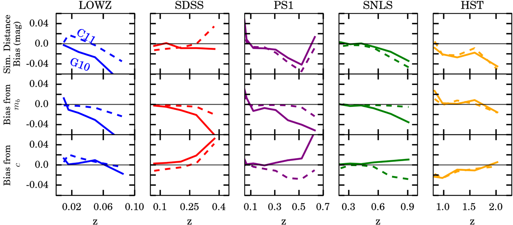
Figure 23. Same as Figure 7, but for the combined Low-z sample.
Download figure:
Standard image High-resolution image
Table 18.
Efficiency of Low-z Samples. The Efficiencies of the low-z Surveys. These Efficiencies Combine the Detection and Spectroscopic Selection Efficiencies. The Parameters  Describe the Parameters of Appendix C Equation (13). The Sys-Efficiency is the 1σ 3D Shift in Best-fit Parameters
| Surv | Efficiency ( ) ) |
Sys-Efficiency ( ) ) |
|---|---|---|
| CfA3 | 15.1, 1.1, 0.1 | 14.7, 1.3, 0.1 |
| CfA4 | 13.6, 1.45, 0.3 | 11.2, 2.05, 0.7 |
| CSP | 10.9, 2.1, 0.9 | 12.5, 2.0, 0.2 |
| CfA1&CfA2 | 12.5, 1.55, 0.9 | 11.9, 1.65, 0.8 |
Download table as: ASCIITypeset image
Furthermore, we find that to optimize the match of Low-z MC to the data, we must change the functional form that expresses the underlying stretch population. As discussed for Table 3, we define the population by an asymmetric Gaussian. However, in Figure 23, the x1 distribution is bimodal. Therefore, we express the population as the combination of two asymmetric Gaussians. Using the same process as in SK16, the x1 distributions for the Low-z sample are found to be  for the first mode and
  for the second mode.
Finally, the alternative to a magnitude-limited survey is a volume-limited survey. This is discussed in detail in S14, but to reproduce the trends of c and x1 with redshift shown in the bottom panel of Figure 23, we need to put in a redshift dependence of the mean c and x1 that is caused by evolution of demographics. We find the dependence, which is roughly the slope of the trends in Figure 23, to be Δc = −1.0 × Δz and  .
.
One other approach to model the Low-z sample is to study the host galaxy demographics. As discussed in Section 5.3, there is a large imbalance between high- and low-mass host galaxies at low z. Pan et al. (2014) analyzed the PTF low-z SN sample, which is a rolling and not galaxy-targeted sample, and found that there was a strong imbalance of the number of high- and low-mass host galaxies (56/26 for mstep = 10.0 and 48/34 for mstep = 10.13). It is not as large as that shown for the Low-z sample in Figure 14; however, it gives a better sense of how much the targeting of galaxies skewed the distribution. This information can be used with relations between host galaxy mass and SN properties to try to infer characteristics of the Low-z SN sample.
Footnotes
- 22
y-band observations are taken during bright time but are not used in this analysis.
- 23
- 24
- 25
SNANA_v10_50a.
- 26
- 27
This has no relation to β from Equation (3).
- 28
CSP SN photometry had unrealistically small (down to 0) photometric uncertainties, so we added an error floor of 0.01 mag consistent with other surveys.