


Abstract
Element abundances in the solar photosphere, chromosphere, transition region, and corona are key parameters for investigating sources of the solar wind and for estimating radiative losses in the quiet corona and in dynamical events such as solar flares. Abundances in the solar corona and photosphere differ from each other depending on the first ionization potential (FIP) of the element. Normally, abundances with FIP values less than about 10 eV are about 3–4 times more abundant in the corona than in the photosphere. However, recently, an inverse FIP effect was found in small regions near sunspots where elements with FIP less than 10 eV are less abundant relative to high FIP elements ( eV) than they are in the photosphere. This is similar to fully convective stars with large starspots. The inverse FIP effect is predicted to occur in the vicinity of sunspots/starspots. Up to now, the solar anomalous abundances have only been found in very spatially small areas. In this paper, we show that in the vicinity of sunspots there can be substantially larger areas with abundances that are between coronal and photospheric abundances and sometimes just photospheric abundances. In some cases, the FIP effect tends to shut down near sunspots. We examine several active regions with relatively large sunspots that were observed with the Extreme-ultraviolet Imaging Spectrometer on the Hinode spacecraft in cycle 24.
Export citation and abstract BibTeX RIS

Original content from this work may be used under the terms of the Creative Commons Attribution 3.0 licence. Any further distribution of this work must maintain attribution to the author(s) and the title of the work, journal citation and DOI.
1. Introduction
Solar and stellar coronal abundances differ from their photospheric abundances due to the so-called First Ionization Potential Effect (FIP; e.g., Laming 2015). In the solar case extreme-ultraviolet (EUV) and X-ray spectroscopy observations show that the solar coronal abundances of low FIP elements (less than about 10 eV) are about a factor of three to four times greater than the abundances of high FIP elements than is the situation in the photosphere (e.g., Feldman 1992; Schmelz et al. 2012). Similar abundance differences between the photosphere and corona are also detected by in situ observations (Meyer 1985; Reames 2014). The abundances of the high FIP elements are believed to be the same in the corona as in the photosphere. In some stellar atmospheres, this situation is reversed (inverse FIP effect), with the low FIP elements being seemingly depleted in the atmosphere relative to the high FIP elements (e.g., Brinkman et al. 2001; Drake et al. 2001; Wood et al. 2012; Wood & Laming 2013). In the stellar case, stars with the inverse FIP effect generally have heavy starspot populations. Starspots can be much larger than typical solar sunspots (e.g., Vogt & Penrod 1983), which might be too small to be detectable on other stars. However, the configuration of magnetic fields in the vicinity of sunspots might be similar to the configuration in starspots.
Recently, Doschek et al. (2015) and Doschek & Warren (2016) discovered an inverse FIP effect in small regions near sunspots in analyzing spectra from the Extreme-ultraviolet Imaging Spectrometer (EIS; Culhane et al. 2007) on the Hinode spacecraft (Kosugi et al. 2007). Although coronal abundance anomalies that do not conform to the average FIP predictions have been known for some time (e.g., Schmelz et al. 1996; Phillips et al. 2015), no clear case consistent with Laming (2015) predictions for the inverse FIP case had been previously reported for solar coronal abundances.
Solar coronal abundance determinations are rather difficult to make. All work depends on the accuracy of atomic data for excitation cross-sections, radiative transition probabilities, and ionization and recombination cross-sections. Almost all of the atomic data (with the exception of the experimentally determined atomic energy levels) is theoretical, and little has been verified by laboratory experiments. The stellar abundance measurements that indicate an inverse FIP effect are obtained from X-ray spectra from spacecraft such as the European Space Agency's X-ray Multi-Mirror Mission (XMM-Newton) (e.g., Kahn et al. 2001; Jansen et al. 2001) and the Chandra X-ray Observatory (CXO; e.g., Tananbaum et al. 2014). Some key high FIP lines are resonance transitions in He-like Ne ix, H-like Ne x, and similar lines for He-like and H-like O vii and O viii. There are many low FIP lines of highly ionized iron (Fe xvii–Fe xxiv) to compare with the Ne and O line intensities. In the solar case, the same high and low FIP X-ray lines have also been used, including also lines of Ar xvii, K xix, Ca xx, and Fe xxv. In addition to EIS, there are also extreme-ultraviolet abundance measurements (e.g., Young & Mason 1997; Feldman & Laming 2000) from instruments such as the Coronal Diagnostic Spectrometer (CDS; Harrison et al. 1995) and the Solar Ultraviolet Measurements of Emitted Radiation (SUMER) spectrometer (Wilhelm et al. 1995) on the Solar and Heliospheric Observatory spacecraft (Domingo et al. 1995). Thus a large number of different atomic systems with different accuracies in the atomic data have been used to determine abundances. All the determinations also depend on an assumption regarding the equilibrium state of the atmosphere. Nevertheless, in spite of all the uncertainties, the abundance measurements do converge to cases where a real or inverse FIP situation is valid.
The Laming (2015) model for the FIP effect posits that the ponderomotive force in the presence of waves propagating through the atmosphere leads to the fractionation of low and high FIP elements in the chromosphere. The model can explain both the FIP and inverse FIP cases. The Laming (2015) model predicts high variability in the FIP effect because the conditions necessary for it are expected to be highly variable. However, in the solar atmosphere, the low FIP elements in the corona tend to cluster around an abundance that is about three to four times greater than in the photosphere. This result may be due in part to a paucity of measurements in different regions of active regions, flares, and the quiet Sun, or there may be a self-regulatory mechanism that limits the range of FIP variability, similar to the average temperature of the quiet-Sun corona (about 1.4 × 10⁶ K), which seems fairly constant over the entire quiet-Sun solar atmosphere.
Because the inverse FIP effect seen in the solar atmosphere is located near sunspots, consistent with stellar results, in this paper, we investigate active regions with relatively large sunspots to look for FIP variability. Since some small regions can show an inverse FIP effect, it may be possible that either photospheric abundances or abundances between photospheric and coronal abundances might be found in other areas of active regions. Using EIS observations, mostly chosen because they are of active regions with large sunspot groups, we have found elemental abundances that vary from coronal to inverse FIP over substantial parts of the raster field of view. In one case, we can investigate temporal abundance variations. This paper describes the results. Section 2 briefly describes the EIS instrument. Section 3 describes the method for determining an FIP effect with EIS spectra, and the remaining sections describe the results for each region analyzed. A list of the regions discussed below is given in Table 1.
Table 1. Regions Observed
| Date | EIS file | Active Region |
|---|---|---|
| 2014 Feb | EIS_l1_20140201_125441 | 11967 |
| 2014 Feb | EIS_l1_20140202_122934 | 11967 |
| 2014 Feb | EIS_l1_20140202_141952 | 11967 |
| 2014 Feb | EIS_l1_20140203_113540 | 11967 |
| 2014 Feb | EIS_l1_20140205_124534 | 11967 |
| 2014 Oct | EIS_l1_20141024_101349 | 12192 |
| 2016 Feb | EIS_l1_20160215_103336 | 12496 |
| 2012 Mar | EIS_l1_20120309_030933 | 11429 |
| 2012 Jun | EIS_l1_20120613_110535 | 11504 |
Download table as: ASCIITypeset image
2. EIS Spectra
The EIS spectrometer is described in detail by Culhane et al. (2007). EIS observes two wavelength bands between about 170–213 Å and 250–290 Å. A multi-layer coated telescope images the Sun onto one of four possible slit/slot apertures oriented in the north–south direction. Light passing through a slit/slot is diffracted by a multi-layer coated grating and is imaged onto two CCD detectors. Narrow wavelength windows can be selected within the wavebands. Up to 25 spectral lines can be observed. Alternatively, a full-CCD study can be selected, i.e., the entire waveband is recorded. We use a data set of full-CCD studies of active regions obtained using two studies called ATLAS_30 and ATLAS_60.
ATLAS_60 uses the 2'' slit and makes a 120'' × 160'' nominal field-of-view raster with 2'' steps and 60 s exposures. ATLAS_30 has the same parameters as ATLAS_60 except that the exposure times are 30 s. The EIS spectra have been processed using standard EIS software for dark current, the CCD pedestal, warm pixels, slit tilt, and temperature variations due to the Hinode orbit. We used the old EIS calibration instead of the new calibrations discussed by Del Zanna (2013) or Warren et al. (2014). The argon and calcium lines near 194 Å used to determine whether or not an inverse FIP effect is observed are so close in wavelength that the original calibration is completely sufficient.
3. Measuring The FIP Effect
Determining abundances with EIS is described in Feldman et al. (2009). The EIS spectra have a number of Ar lines (Doschek & Warren 2016). Ar has the third highest FIP (15.76 eV) after He and Ne. Ca has a low FIP (6.11 eV). Thus, if a Ca and Ar line could be found and each line had the same temperature dependence in ionization equilibrium, and electron density was not a significant factor, then the ratio of these two lines would depend primarily on the abundance of argon to the abundance of calcium, a direct measure of the FIP effect. Two lines nearly satisfying this condition are the Ar xiv line at 194.40 Å and the Ca xiv line at 193.87 Å. The intensity ratio of the contribution functions as a function of temperature and density for these lines is shown in Figure 1 for coronal and photospheric abundances. In ionization equilibrium Ca xiv and Ar xiv are formed near 3.6 MK. Note the weak dependence on temperature over a relatively large temperature range. Note also that as the density increases, the ratio decreases, causing the abundance ratio to appear more coronal.

Figure 1. Intensity ratios of the contribution functions of the Ar xiv and Ca xiv lines as a function of electron temperature and electron density. The ratios are shown for coronal and photospheric abundances. The vertical lines denote the minimum (3.8 MK) and maximum (4.8 MK) temperatures that we consider plausible due to temperature variations in the plasma at the temperature of formation of the Ar xiv and Ca xiv lines. The temperature range was determined from the intensity ratio of a Ca xv line at 200.97 Å to the Ca xiv line at 193.87 Å.
Download figure:
Standard image High-resolution imageThe intensity ratio of the lines is done using the ionization equilibrium and atomic excitation data in CHIANTI (Dere et al. 1997). We adopt the Ca photospheric abundance given by Caffau et al. (2011) and the Ar photospheric abundance given by Lodders (2008). In the usual FIP effect, the coronal Ar abundance is assumed to be the same as in the photosphere. The coronal Ca abundance can be taken from either Feldman (1992) or Schmelz et al. (2012).
In the case of coronal abundances, the top panel of Figure 2 shows a typical spectrum with the Ar xiv and Ca xiv lines. When abundances are coronal, the Ar xiv/Ca xiv intensity ratio is about 0.25. Note the closely blended feature marked as Ni xvi (194.04 Å) and Ar xi (194.09 Å). In the coronal panel the Ni line is strongest. The bottom panel of Figure 2 shows an example of an inverse FIP effect spectrum. The Ar xiv line is about 1.5 times stronger than the Ca xiv line, and the Ar xi line is now stronger than the Ni xvi line. If the Ar xiv and Ca xiv lines have equal intensity, the abundance is photospheric.

Figure 2. Top panel: a typical coronal abundance spectrum. The Ar xiv/Ca xiv intensity ratio is about 0.25. Bottom panel: an example of an inverse FIP spectrum. The Ar xiv line is about 1.5 times more intense than the Ca xiv line. Equal intensities signify a photospheric abundance. The X and Y quantities are the locations of the spectra in the raster image and will be discussed later.
Download figure:
Standard image High-resolution imageThe spectral range shown in Figure 2 is best for looking for the inverse FIP effect because the high temperature Ar and Ca lines are formed at the same temperature. Other Ar lines are not close to lines formed at a similarly very close temperature and therefore intensity variations can be quite sensitive to temperature. We will discuss some other Ar lines in the next section.
4. The 2014 February 1–5 Active Region Raster
A large sunspot group crossed the solar disk in 2014 February. EIS obtained five full-CCD rasters near areas of the sunspots using the ATLAS_30 study on February 1, 2, 3, and 5. Thus the data can be used to investigate abundance variations over part of the active region and also to investigate abundance variations in this region over a several day interval. The specific EIS files are given in Table 1 and Figure 3 shows the position of the EIS rasters in relation to the sunspots. These data are from the Atmospheric Imaging Assembly (AIA) instruments on the Solar Dynamics Observatory (SDO). The duration of each raster was only 30 minutes. No large flare occurred during the rasters.

Figure 3. EIS raster position relative to the sunspots seen in an AIA 4500 filter image. The EIS files are shown in the figure.
Download figure:
Standard image High-resolution imageThis active region produced a clear inverse FIP effect over a small area. One of the spectra has been shown above in Figure 2 (bottom panel). The Ar xiv/Ca xiv ratio is 1.5. There were two rasters on February 2. Only the earlier raster showed a clear inverse FIP effect. The later raster showed a clear pure photospheric abundance (Ar xiv/Ca xiv) ratio = 1.0). However, on February 3 the inverse FIP effect reappeared and a small area was found with a Ar xiv/Ca xiv ratio of 1.3. This is a marginal inverse FIP effect. The February 3 raster has considerable data drop-out.
There are other Ar lines that can be used to look for the inverse FIP effect. Spectra from two wavelength regions that exhibit coronal abundances are shown in Figure 4. The top panel shows two argon lines and a line of S xi, which is usually assumed to be high FIP. As mentioned, Ar xiv is formed near 3.6 MK. Ar xi and S xi are formed near 1.6 MK. The low FIP iron lines are formed near 1.4 MK. It is not as simple to detect departures from coronal abundances because the high FIP argon and sulfur lines are not formed at exactly the same temperature as the lower FIP iron lines. This is especially true for the Ar xiv line. The Ar xiv line has other problems as well. If a flare is occurring, the line might be blended with a line of Fe xxi, depending on where the spectrum is relative to the main area of the flare. When the temperature of the corona is so low that 3.6 MK plasma is absent, there is still a line at the wavelength of the Ar xiv line. This is a weak unidentified cool line (Brown et al. 2008).

Figure 4. Spectra exhibiting Ar xiv and Ar xi lines with coronal abundances. The X and Y quantities are the locations of the spectra in the raster image to be discussed.
Download figure:
Standard image High-resolution imageThe bottom panel shows another spectrum that contains high FIP sulfur and argon lines along with an Fe xii line. As in the top panel, it is somewhat complicated to compare intensity ratios directly because the lines are formed at different temperatures.
The inverse FIP case shown in Figure 2 is shown in Figure 5 for the spectral regions in Figure 4. In the top panel of Figure 5 the Ar xiv, Ar xi, and S xi lines are all stronger relative to the iron lines than in Figure 4. In the high FIP interpretation, the high FIP elements are not stronger because of a greater abundance. The abundance is assumed to be the same as the coronal abundance case, i.e., a photospheric abundance. Rather, the iron lines are depressed relative to the high FIP lines because the ponderomotive force points toward the Sun instead of away from it (Laming 2015). In our previous observations of inverse FIP regions, S xi did not exhibit the effect and behaved instead like a low FIP ion. In the present case, sulfur is exhibiting a high FIP behavior. Both cases for sulfur can be consistent with the Laming (2015) model, depending on the location of the fractionation.

Figure 5. Spectra exhibiting Ar xiv and Ar xi lines with inverse FIP abundances. The X and Y quantities are the locations of the spectra in the raster image to be discussed.
Download figure:
Standard image High-resolution imageFinally, note how much wider the Fe xii feature is in the bottom panel of Figure 5 compared with Figure 4. This is due to the presence of an enhanced Ar xi line at 190.96 Å (Brown et al. 2008).
In order to show that the different low and high FIP intensities really correspond to an FIP effect, and not variations in the differential emission measure, and to show the extent of the inverse FIP region, we compare several intensity ratios to the high FIP raster images in Figure 6. The top panels show the ratios of high FIP lines to low FIP lines formed at about the same temperature, thus minimizing differential emission measure effects. The bottom panels show the images of the raster in the indicated high FIP lines. Vertical lines are data losses in the raster and the horizontal line in the top middle panel is dust on the CCD. The S x line at 264.233 Å and the Fe xiv line are formed on a different CCD than the other lines. This CCD is displaced from the other CCD along the north–south direction (Y coordinate) by about 17''. The data in Figure 6 have been shifted to account for this and this produces the dark regions seen most clearly on the bottom parts of the Ar xi/Fe xiv and S x/Fe xi panels. The coordinates X and Y given in Figures 2, 4, and 5 are the X and Y coordinates in Figure 6, with Y along the north–south direction and X in the east–west direction.

Figure 6. Top panels: intensity ratios of high FIP to low FIP spectral lines formed at about the same temperature. Bottom panels: intensity images in the indicated high FIP spectral lines. The X in the middle panel is the location of the maximum value of R (1.64, see the text). The high values of R between 70% and 90% of 1.64 surround this position, see the text for details.
Download figure:
Standard image High-resolution imageNote that the peak intensities of all the ratios occur at about the same location in each panel, and that there is no relationship to the intensities in the bottom panel images. This indicates that the apparent increased intensities of the high FIP lines in the small areas shown in the top panels of Figure 6 are due to abundance differences, and not differential emission measure effects.
It is interesting to investigate the abundances over neighboring areas around the inverse FIP region, and we also extend the analysis of the inverse FIP effect and the surrounding rectangular region to the other rasters made within the February active region. We investigate the region enclosed by the rectangle with the white outline in the top middle panel of Figure 6. The region below the horizontal dust area has mostly low temperatures and only weak 3–4 MK emission. We only discuss some results for this region for the February 5 raster. Figure 3 shows that the position of the February 5 raster is shifted northward relative to the other rasters.
The results for the five rasters are given below (for brevity, the intensity ratio Ar xiv/Ca xiv is called R). The coordinates are the coordinates used in Figure 6.
(1) February 1 raster: Between X = 0 and 46 and Y = 100 and 159, the average R is 0.50 (For a coronal abundance R is about 0.24 and for a photospheric abundance R is about 1.0). The maximum R is 1.24 at X = 38, Y = 126. Between X = 54 and 110 and Y = 100 and 159 the average R = 0.46, and the maximum R is 0.80 at X = 54 and Y = 131.
(2) February 2 raster (12:29:34 UT): Between X = 0 and 118 and Y = 100 and 159 the average R = 0.60. The maximum R = 1.64 at X = 38, Y = 122.
(3) February 2 raster (14:19:52 UT): Between X = 0 and 118 and Y = 100 and 159 the average R = 0.50. The maximum R = 1.01 at X = 42, Y = 107.
(4) February 3 raster: Between X = 28 and 36 and Y = 100 and 159 the average R = 0.54. The maximum R is 1.28 at X = 36, Y = 107. There are many data gaps.
(5) February 5 raster: Between X = 0 and 118 and Y = 98 and 159 the average R = 0.42. The maximum R = 0.85 at X = 30, Y = 98. Between X = 0 and 118 and Y = 60 and 87 the average R = 0.42. The maximum R is 0.94 at X = 30, Y = 87.
From the above results, there are some general conclusions that can be reached concerning the February active region. These are as follows.
(6) Another inverse FIP effect has been found. It is not found in every raster but appears in three rasters obtained two days apart.
(7) The inverse FIP effect is only found in a small part of the raster. For the February 2 case (12:29:34 UT), the maximum R = 1.64 and is within 90% of this value for only three pixels between X = 20 and 40 and Y = 100 and 140. There are 12 pixels for which R is within 80% of the maximum, and there are 41 pixels for which R is within 70% of the maximum.
(8) An FIP between coronal and photospheric is found over a large part of the raster for all of the rasters (except February 3, where there are large data gaps) between roughly X = 0 and 118 and Y = 100 and 159. This is a result with the implication that sometimes, near sunspots, the FIP effect tends to shut down. Feldman et al. (1990) made a similar suggestion based on analyses of a single rocket spectrum recorded in July 1975 by the Naval Research Laboratory High Resolution Telescope and Spectrograph (HRTS). The same spectrum was further analyzed by Doschek et al. (1991) who reached the same basic conclusions presented by Feldman et al. (1990). The HRTS results refer to transition region plasma, and it was not possible to say for certain that the plage regions had coronal abundances, though this was implied by both Feldman et al. (1990) and Doschek et al. (1991). If the transition region has photospheric abundances in active regions, then the HRTS sunspot spectrum had inverse FIP abundances. These results imply that the abundance effects we are seeing in the corona extend down to lower transition region temperatures because the HRTS spectral lines observed by Feldman et al. (1990) and Doschek et al. (1991) are formed at temperatures less than about 0.2 MK.
(9) For the 2014 February active region, sulfur also appears to behave as a high FIP element along with lines of argon.
(10) SDO movies show emerging flux and a substantial change in the leading sunspot between February 1 and 5. The EIS rasters were not made during any large flare but there is some flaring activity within the EIS active region as revealed by SDO 131 filter observations and ground-based observations. The two rasters with an inverse FIP effect were made close to the occurrence of small flares. The February 2 and 3 flares occur close to the raster time.
5. An EIS Sit&Stare Observation of the Largest Sunspot of Cycle 24
In a Sit&Stare study, the EIS north–south slit is placed at a location on the Sun, and EIS takes multiple exposures. The slit tracks the differential rotation of the Sun. The largest sunspot of Cycle 24 was observed on 2014 October 24 with a Sit&Stare study called hpw009_fullccd_sas. The purpose of this observation was to investigate temporal abundance variations over the region within the field of view of the slit. In this study, the slit size is 1'' and the field of view is 1'' × 128''. The exposure times are 25 s and 115 exposures were obtained. The start time was 10:13:49 UT and the end time was 11:03:20 UT. The position of the slit is shown in Figure 7 relative to AIA data.

Figure 7. Position of the Sit&Stare slit relative to the sunspot seen in an AIA 4500 filter image.
Download figure:
Standard image High-resolution imageThe Ar xiv/Ca xiv intensity ratio was measured and the ratio is displayed in Figure 8 in a time plot. In this figure, the intensity variations of the ratio along the slit can be seen as a function of time. The intensity ratio varies between coronal and about 0.44 over the entire raster. The brighter regions have the highest ratios. The brightest region, between Y = 55 and 58, has an average ratio of 0.44. The faintest region between Y = 0 and Y = 8 has an average ratio of 0.30. The average ratio between Y = 55 and Y = 90 is 0.41.

Figure 8. Time plot of the Ar xiv/Ca xiv intensity ratio variations along the slit length in arcsecs. Each exposure is 25 s long and exposures began at 10:13:49 UT. The white and black vertical lines are data dropouts.
Download figure:
Standard image High-resolution imageThe intensity ratios in Figure 8 can be compared to the Ca xiv intensity in Figure 9. The highest ratios in the top panel appear to occur coincident with the brightest Ca xiv intensity regions. However, careful inspection will reveal that the two bright regions are not coincident, but just next to each other. There appears to be an inverse correlation with intensity over the whole length of the slit.

Figure 9. Top: a section of the slit showing Ar xiv/Ca xiv intensity variations for the 2014 October 24 raster shown in Figure 8. Bottom: the Ca xiv intensity variations along the same slit segment. The white and black lines are data dropouts.
Download figure:
Standard image High-resolution imageThe conclusions from the Sit&Stare data are as follows.
(1) The Ar xiv/Ca xiv ratio is somewhere between photospheric (1.0) and coronal (0.25) over the entire slit length throughout the duration of the observation. Again it appears that the presence of sunspots tends to lessen the FIP effect. This is broadly consistent with starspot observations and the stellar inverse FIP effect.
(2) The intermediate FIP effect and the inverse FIP effect do not occur in high emission line intensity regions.
The apparent abundance variations described above are not nearly as large as for the inverse FIP cases we have found. They also did not vary much in time over the observation period. The inverse FIP cases are so large that temperature cannot explain the results. However, note that Figure 1 shows a variation of ratio with temperature. When the ratio varies from about 0.2 to about 0.4, the possibility that this is due to temperature must be considered. Statistical errors in the ratios are at most about 20% and therefore are not significant (see the next section). The possibility of temperature variations is discussed in the next section after presenting similar results as obtained in this section.
6. The Active Region Raster on 2016 February 15
This active region was observed on 2016 February 15 using a study called hpw021_vel_240 × 512v1. This region was chosen because a flare occurred during the raster. This is not a full-CCD study but examines 25 windows containing at least 25 lines of interest. The field of view is 240'' × 512'' and the 1'' slit is used. However, the raster step size is 2''. Exposure times are 60 s. The EIS raster we examine began at 10:33:36 UT. The position of the raster in the active region as seen in an AIA 4500 filter image is shown in Figure 10.

Figure 10. EIS raster position relative to the active region and sunspots as seen in an AIA 4500 filter image.
Download figure:
Standard image High-resolution imageAn M1.1 flare occurred at about the time the raster started. The GOES light curve is shown in Figure 11. The event appears to be a multiple event judging from the rise curve. Fortunately, the high temperature part of the flare occurred nearly over the center of the EIS raster. We wish to investigate departures from coronal abundances in this active region while it was flaring. Departures similar to the examples shown above are regions where the Ar xiv/Ca xiv ratio is between about 0.3 and 1, the photospheric ratio. The usual coronal abundance ratio is between 0.2 and 0.3. We did not find an inverse FIP region in the EIS raster portion of the active region.

Figure 11. GOES light curves for the 2016 February 15 EIS raster.
Download figure:
Standard image High-resolution imageWe decided to limit the investigation to areas near the flare because of statistical considerations, i.e., we generated a sub-raster. Also, when the 3–4 MK plasma is weak relative to lower temperature plasma, three weak lines appear rather strongly on the blue wing of the Ar xiv line and the two neighboring lines near the Ca xiv line make accurate Ca xiv intensities difficult. Therefore, we have made three-Gaussian fits to both the calcium and the argon lines to improve the accuracy of their intensity ratio.
To search for abundances between coronal and photospheric, we selected all ratios between values of 0.35 and 0.5. Initial inspection indicated that ratios above 0.5 would be absent. We then initialized a blank image the size of the chosen sub-raster. In this image, all pixels that do not satisfy the ratio restriction were left at values of zero. All pixels that satisfy the restriction were assigned values of 1. We also constructed a similar image where a coronal abundance restriction was imposed, i.e., find all ratios between values of 0.2 and 0.3. The results are shown in Figure 12.

Figure 12. Left panel: a sub-raster image in the Ca xiv line at 193.87 Å for the 2016 February 15 active region raster. Middle panel: the intensity ratio of the Ar xiv 194.40 Å line and the Ca xiv line subject to the condition that the ratios fall between 0.35 and 0.5. There are 510 pixels that satisfy this condition and they are given an intensity of 1. All other pixels have 0 intensity. Right panel: the same ratio with the condition that values fall between 0.2 and 0.3. There are 3007 pixels that satisfy this condition. Note that the X-axis is a stacking of exposures. Each exposure is separated by 2'' from its neighbors.
Download figure:
Standard image High-resolution imageThe left panel of Figure 12 is an image of the sub-region we chose in the Ca xiv line. the brightest areas correspond closely to the brightest region in a high temperature line of Fe xxiv. This is the main area of the flare. The middle panel shows the pixels that satisfy the condition that the Ar xiv/Ca xiv ratio is between 0.35 and 0.50. There are 510 such pixels. The right panel shows the coronal abundance case (0.2–0.3) and here there are 3007 pixels.
The right panel of Figure 12 shows that most of the image is dominated by ratios that satisfy the standard coronal abundance. Even the heart of the flare region exhibits coronal abundances. This result is consistent with Del Zanna & Woods (2013) and Warren (2014) who in general obtained coronal abundances for active regions. The total number of pixels in the panel is 5353 so 56% of the pixels satisfy the coronal abundance criteria. The dark gaps in the right panel are regions where the ratio is not between 0.2 and 0.3. There are also some regions where the temperature is less than 3–4 MK and Ca xiv and Ar xiv emission are absent.
The middle panel has roughly two distributions of pixels that exhibit ratios between 0.35 and 0.5. There are isolated single pixels. We assume that these are just statistical fluctuations and do not represent real abundance differences. However, there are two rather conspicuous clumps of pixels that indicate non-coronal abundances (Box A and Box B). Inspection of individual spectra indicates that these regions are areas where the abundance truly deviates from a pure coronal value.
To see this result more clearly, and to compare it not only with Ca xiv emission, but also with Fe xxiv hot flare emission, we plot in Figure 13 the images of these two lines along with an image of the ratio regardless of value and the middle panel of Figure 12. In Figure 13 the data are plotted taking into account the 2'' step size, so the X-axis is now in arcseconds.

Figure 13. Top left: an image of the flare region in Ca xiv in the 2016 February 15 active region raster. Top right: the Ar xiv/Ca xiv intensity ratio. Bottom left: the Ar xiv/Ca xiv ratio between 0.35 and 0.50. Bottom right: an image in the Fe xxiv line near 255 Å.
Download figure:
Standard image High-resolution imageCareful inspection of Figure 13 shows that the peaks in the Ar xiv/Ca xiv ratio do not fall in the bright regions of the Fe xxiv line. They are adjacent to the bright flare regions. They could be flare footpoint regions. The Ca xiv region is also not completely coincident with the Fe xxiv region.
We investigate the clumps in the middle panel of the Figure 12 image by determining how many pixels have ratios between 0.37 and 0.50 and how many pixels are outside of this range. We increase the lower limit of the ratio slightly from 0.35 to 0.37 to be well outside the normal range of the average coronal abundance ratio. This gives an indication of the suggestive impression that the abundances in the two clumpy regions are actually between coronal and photospheric abundances. The result is shown in Figure 14 for the Box A region in Figure 12. The average over the entire image is also indicated.

Figure 14. Ar xiv/Ca xiv ratio over Box A in Figure 12 (2016 February 15 active region) with the X and Y coordinates indicated. These coordinates are the coordinates of the middle panel image in Figure 12. The stars all have ratios greater than 0.37. Ratios greater than this are considered as potentially produced by abundance variations. The lower horizontal line is the average ratio over the entire Figure 12 image.
Download figure:
Standard image High-resolution imageFigure 14 shows that the majority of the pixels (68 pixels) in the small region have Ar xiv/Ca xiv ratios (0.37–0.50) that are between coronal and photospheric. There are 31 pixels with ratios outside of this range. About half of these are on the high side of coronal abundances. Because the increased ratio is much smaller than the photospheric and inverse FIP ratios found in some of the other regions, we investigate the possibility of a temperature explanation more closely.
The intensity ratio of a Ca xv line at 200.97 Å to the Ca xiv line at 193.87 Å is temperature sensitive. There is a close blend of the Ca xv line with an Fe xiii line, which we have removed with Gaussian fitting. We can compare the calcium line ratios to the argon to calcium ratios we see in Figure 14. If there is a systematic difference in the calcium ratios between the starred and diamond ratios in Figure 14, then we can suspect temperature variations as a possible cause of the high Ar xiv/Ca xiv ratios.
The result of the comparison for Box A is shown in Figure 15. There is a lot of scatter, but the results basically show a good overlap with all of the Ar xiv/Ca xiv ratios, indicating that temperature is not a significant factor in producing the differences we feel are due to abundance variations.
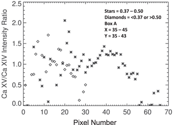
Figure 15. Ca xv/Ca xiv ratios (the temperature proxy) for the Box A region illustrated in Figure 14 (2016 February 15 active region).
Download figure:
Standard image High-resolution imageWe have repeated the same analysis for the smaller clumpy Box B region in Figure 12 near X = 15, Y = 35. The results are shown in Figure 16 and are quite similar to those shown in Figure 14. Even the spectra that fall at ratio values less than 0.37 still on average have somewhat greater values than the majority of the coronal abundance spectra in the active region. This can be seen in Figure 17, where we show a histogram distribution of intensity ratios over the entire image shown in Figure 12.

Figure 16. Ar xiv/Ca xiv ratio over the Box B area in Figure 12 (2016 February 15 active region).
Download figure:
Standard image High-resolution image
Figure 17. Histogram of the Ar xiv/Ca xiv intensity ratio over the entire image shown in Figure 12 (2016 February 15 active region).
Download figure:
Standard image High-resolution imageThe statistical errors in Figures 14–16 are not significant. This can be seen in Figure 18, where we show in the top panels images and ratios involving the Ar xiv, Ca xiv, and Ca xv lines. The horizontal dotted line in the top panels is a slice through the regions discussed above and the bottom panels show the important ratios along the slice with error bars. In the bottom panels, the horizontal dotted line for the Ar xiv/Ca xiv ratio is the coronal abundance value. The dotted lines in the right lower panel are the Ca xv/Ca xiv ratios at 4 and 5 MK. It can be seen that the statistical errors in the Ar xiv/Ca xiv ratios are small compared to the deviations in the ratio we have been discussing. Also, there is no correlation between the Ar xiv/Ca xiv and Ca xv/Ca xiv ratios.
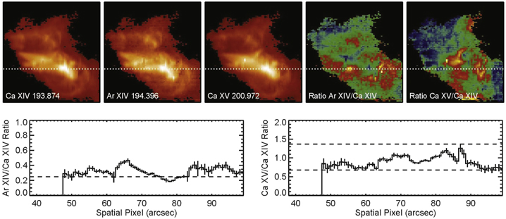
Figure 18. Images and ratios with indicated statistical error bars (2016 February 15 active region). The dotted horizontal line in the top panels is a slice through the regions discussed in the text. The ratios in the lower panels are the ratios through this slice. The horizontal dotted lines in the bottom panels are the average coronal abundance Ar xiv/Ca xiv ratio and the Ca xv/Ca xiv ratio at 4 and 5 MK.
Download figure:
Standard image High-resolution imageThe ratios we obtain for this active region are about the same as for the Sit&Stare case discussed in the previous section. We find no correlation of the Ar xiv/Ca xiv abundance ratio with the Ca xv/Ca xiv ratio in any of the data. The correlation coefficient is near zero. The Ca xv/Ca xiv ratio varies between about 0.6 and 1.2 in all the data, whether or not an apparent abundance variation is seen. Using CHIANTI, these ratios correspond to log temperatures of about 6.58 and 6.68. These temperatures are noted as vertical lines in Figure 1. The average ratio between about 0.8–1.0 corresponds to a temperature of about 6.64. From Figure 1, it can be seen that only an Ar xiv/Ca xiv ratio of about 0.3 might be explained by a variation of temperature in a coronal abundance plasma at any of the densities shown in the figure. Ratios of 0.4 and 0.5 are outside the boundaries of the vertical lines in Figure 1.
In summary, even in an active region for which there is no inverse or purely photospheric abundance regions, there can still be small regions in which the abundances at 3–4 MK are somewhere in between pure coronal and pure photospheric abundances.
7. The 2012 March 9 Flare
EIS observed a fairly intense flaring active region on 2012 March 9 using the ATLAS_30 full-CCD study. The flares in this region have been extensively discussed (e.g., Doschek et al. 2013; Polito et al. 2017). This flare also exhibited a sunquake (A. Kosovichev, 2013, private communication). We revisit this region to investigate the FIP effect.
As in other cases, we find an area with abundances between photospheric and coronal near a large sunspot. Figure 19 shows the region near the sunspot. The top panels are AIA and Helioseismic and Magnetic Imager (HMI) data. The bottom left panel shows the area where the Ar xiv/Ca xiv ratio is between 0.45 and 0.6. Note the converging flux lines toward the sunspot in the top left panel. This region appears to be spatially coincident with the larger than coronal ratios. The bottom right panel shows the approximate locations of the sunspots mapped onto an image in the Ca xiv line.

Figure 19. Part of the 2012 March 9 active region. Top panels: HMI with AIA images of the flare region. Bottom left panel: the area in the image (white area), where the Ar xiv/Ca xiv ratio is between 0.45 and 0.60. Bottom right panel: an EIS image in the Ca xiv line with the approximate locations of the sunspots (red disks).
Download figure:
Standard image High-resolution image
8. Discussion
We have shown that coronal abundances can exhibit some variability in active regions. Near sunspot abundances that range from coronal to photospheric to inverse FIP can be found over extended regions. As mentioned, prior to the EIS observations, differences in abundances near a sunspot relative to the transition region were found by Feldman et al. (1990) with a follow-up study by Doschek et al. (1991). The inverse FIP regions found so far are quite small in size. The impression is that around sunspots the FIP effect tends to try to shut down. Our observations are primarily in argon and sulfur lines. Argon has a very high FIP, and can always be regarded as a high FIP element, but sulfur is on the border between low and high FIP, and in most cases we have seen around sunspots, sulfur behaves more like a low FIP element. However, we did discuss one case above where sulfur behaves like a high FIP element.
During the writing of this paper, another inverse FIP region was found close to a large sunspot region observed on 2012 June 13 (eis_l1_20120613_110535). In this region, sulfur behaves like a low FIP element. Unfortunately, the inverse FIP region was very close to a blemished region on the CCD. The maximum Ar xiv/Ca xiv ratio is 1.38. As in the other regions discussed, areas with ratios between photospheric and coronal were found. It appears that the raster position probably missed some of the non-coronal abundance areas, so this region was not discussed in detail. However, the results support the conclusions above.
As mentioned, the only model known to the authors that can account for both the FIP and the inverse FIP effect is the Laming (2015) model. In the Laming model the FIP effect is produced by a ponderomotive force acting with Alfvén waves to preferentially transport ions instead of neutrals into the corona. The force points upward from the chromosphere into the corona because the wave gradient points upwards into the corona. However, in some cases acoustic p-mode waves can mode convert to fastmode waves at the point where the Alfvén speed and sound speed are equal. These upward moving converted fastmode waves get reflected back toward the chromosphere and the ponderomotive force is now in a direction toward the chromosphere and the fastmode waves carry the low FIP elements out of the coronal regions into the chromosphere and this results in an inverse FIP effect. Sunspots are known sinks of p-mode energy and the p-modes probably convert to fastmode waves (Braun 1995; Laming 2015). The introduction of mode converted acoustic waves around sunspots would explain why we find the inverse FIP effects always near sunspots and perhaps why over larger regions photospheric or hybrid-type coronal abundances are found.
The Laming (2015) model predicts variability in the sulfur status and also makes other predictions involving neon and oxygen lines. Spectral lines from these elements that could be used for abundance determinations are not available in EIS spectra but, as mentioned before, can be found in X-ray stellar spectra where inverse FIP effects are found through analysis of neon and oxygen lines. For stars with large starspot regions, conditions would seem ideal for the inverse FIP effect to be dominant over most of the surfaces of these stars.
So far, the discussion has focused on the FIP effect causing all of the abundance variations observed. The FIP effect is probably the cause of the inverse FIP regions we have discussed, but some regions, particularly in the 2016 February 15 active region, only show an abundance variation between coronal and photospheric. It is possible that this type of variation is simply due to newly emerged flux. Emerging flux carries plasma from the photosphere into the corona and earlier Skylab transition region observations have shown that, at times close to the emergence time, the abundance of newly emerged plasma is photospheric (Sheeley 1995, 1996). In time, the abundance changes into a coronal abundance, presumably due to the FIP effect. These observations refer to transition region structures, most of which do not connect with the corona. So the situation for coronal plasma is still unclear, but the emergence of magnetic flux probably plays a role in small abundance variations.
Solar and stellar atmospheric abundances are important in astrophysics because stars populate the interstellar media with metals. Abundances are important for calculating radiative losses from all such plasmas. However, perhaps even more important, because the Laming (2015) model makes definite predictions about the distribution of the FIP effect for the solar abundant elements, measurements of the FIP are in effect checks on the complicated calculations of wave generation, propagation, and damping in plasmas under various conditions.
Because conditions in the chromosphere/coronal interface would appear to be enormously variable due to the complex fine structure morphology revealed by AIA and more recently by the Interface Region Imaging Spectrograph (De Pontieu et al. 2014), one might predict that coronal abundances should be highly variable. However, this is not the case. There are other conditions in the solar atmosphere, such as the dominant temperatures in the quiet-Sun (∼1.4 MK) and active regions (∼3–4 MK), that one might also predict should be highly variable, but they are not. The solar atmosphere evidently has some large-scale regulatory mechanisms that control conditions within it. It is highly desirable to pursue solar abundance determinations in the X-ray region (from about 1.7 Å to ∼30 Å), where spectral lines from all the important solar elements are found.
Hinode is a Japanese mission developed and launched by ISAS/JAXA, collaborating with NAOJ as a domestic partner, and NASA (USA) and STFC (UK) as international partners. Scientific operation of the Hinode mission is conducted by the Hinode science team organized at ISAS/JAXA. This team mainly consists of scientists from institutes in the partner countries. Support for the post-launch operation is provided by JAXA and NAOJ, STFC, NASA, ESA (European Space Agency), and NSC (Norwegian Space Center). We are grateful to the Hinode team for all their efforts in the design, build, and operation of the mission.
G.A.D. and H.P.W. acknowledge support from the NASA Hinode program. We thank Drs. Martin Laming and Brian Wood for helpful comments on the manuscript. We thank the referee for a careful reading of the manuscript.