


Abstract
The only Halley-type comet discovered by the Wide-Field Infrared Survey Explorer (WISE), C/2010 L5 (WISE), was imaged three times by WISE, and it showed a significant dust tail during the second and third visits (2010 June and July, respectively). We present here an analysis of the data collected by WISE, putting estimates on the comet's size, dust production rate, gas production (CO+CO2) rate, and active fraction. We also present a detailed description of a novel tail-fitting technique that allows the commonly used syndyne–synchrone models to be used analytically, thereby giving more robust results. We find that C/2010 L5's dust tail was likely formed by strong emission, likely in the form of an outburst, occurring when the comet was within a few days of perihelion. Analyses of the June and July data independently agree on this result. The two separate epochs of dust tail analysis independently suggest a strong emission event close to perihelion. The average size of the dust particles in the dust tail increased between the epochs, suggesting that the dust was primarily released in a short period of time, and the smaller dust particles were quickly swept away by solar radiation pressure, leaving the larger particles behind. The difference in CO2 and dust production rates measured in 2010 June and July is not consistent with "normal" steady-state gas production from a comet at these heliocentric distances, suggesting that much of the detected CO2 and dust was produced in an episodic event. Together, these conclusions suggest that C/2010 L5 experienced a significant outburst event when the comet was close to perihelion.
Export citation and abstract BibTeX RIS
1. Introduction
Comets contain primordial material from the protoplanetary disk, making them excellent resources for understanding the early solar system and other planetary systems. However, comets still have undergone some alterations via different processes, such as impacts and insolation (Prialnik & Bar-Nun 1987), after their relatively recent entry into the inner solar system. These processes can cause significant structural changes in the comet from its original form of conglomerated icy planetesimals on timescales that, for short-period comets, are less than the comet's dynamical lifetime of ∼104–105 yr (Levison & Duncan 1994; Lisse 2002). In order to understand what comets were like when they formed, we therefore must understand how they have evolved over time.
We have seen that comets have a wide variety of volatiles present in their nuclei and comae (Bockelée-Morvan et al. 2004, pp. 391–423; Mumma & Charnley 2011). With each perihelion passage through the inner solar system, a comet undergoes thermal evolution when it receives a significant burden of insolation containing orders of magnitude more energy than during the rest of its orbit (Prialnik & Bar-Nun 1987). The heat from the Sun warms up the comet, causing volatiles to be released and intermixed dust particles to be carried along with the escaping gas. Three primary drivers of cometary volatile activity due to insolation have been identified: H2O sublimation, CO/CO2 sublimation, and the amorphous to crystalline (a-to-c) transition of water ice (Meech & Svoren 2004). The a-to-c transition does not produce any volatiles directly, and thus will not be discussed further here. Water is the most abundant volatile (Festou et al. 2004) but CO and CO2 are significant, ∼10% as abundant on average. Since the three drivers becomes important at different temperatures and heliocentric distances (Meech & Svoren 2004), cometary activity in different thermal regimes is likely dominated by different volatiles. Notably, H2O ice, CO2 ice, and CO ice sublimation can become strong within ∼3, ∼13, and ∼120 au, respectively. Note that the distances listed are not "turn on" points. That is, sublimation of these ices will occur beyond these heliocentric distances, just to a much lesser degree than within them (Cowan & A'Hearn 1979). We note, however, that while it is possible that cometary activity could occur at such large heliocentric distances, few comets have been observed to exhibit such behavior (Meech et al. 2004; Szabó et al. 2008, 2011; Kramer et al. 2014).
Cometary dust tails can be a useful proxy for understanding the volatiles in cometary nuclei. As seen in the recent flyby of comet 103P/Hartley 2, H2O sublimation can cause coma morphology and dust emission that are significantly different from those caused by CO2 sublimation (A'Hearn et al. 2011). This suggests that if the activity on the comet is driven by something other than water, i.e., something that is not the main volatile constituent, the dust grains that are dragged off the nucleus by that volatile may have different properties. The difference in grain properties may be due to the fact that, if CO2 is causing the grains to be lifted off the nucleus, the grains still contain abundant H2O ice in solid form, keeping them bound and large. The grains then proceed to sublimate their H2O ice and fragment into smaller grains, releasing substantial coma gas as they do so.
The Halley-type comet C/2010 L5 (WISE) was discovered at a heliocentric distance of 1.21 au on 2010 June 14 by the Wide-Field Infrared Survey Explorer (WISE) mission (Mainzer et al. 2010), which is described in further detail below. The comet was found to have a perihelion distance (q) of 0.79 au, classifying it as a Near-Earth Object. Its other orbital parameters are as follows: e = 0.90, i = 147 05, TP = 2010 April 23, and orbital period = 23.56 yr (recorded from JPL's Small Body Database (http://ssd.jpl.nasa.gov/sbdb.cgi) on 2015-06-16). In this paper, we present an analysis of comet C/2010 L5 (WISE). The remainder of the paper is structured as follows: Section 2 describes the images used in the analysis; Section 3 describes the analysis techniques used in this work, including the presentation of a novel tail-fitting technique; Section 4 discusses the results obtained and their interpretation; and Section 5 gives conclusions.
2. Data
The infrared data for C/2010 L5 were collected using the WISE telescope (Wright et al. 2010); WISE is a NASA Medium Class Explorer Mission that surveyed the sky between 2010 January and 2011 February (Wright et al. 2010; Mainzer et al. 2011), using a 40 cm diameter telescope, positioned in Sun-synchronous polar orbit. The telescope and detectors were cooled using a solid-hydrogen cryostat, which cooled the telescope down to less than 17 K and the detectors down to 7.8 K.
WISE simultaneously collected data in four infrared bands at wavelengths of 3.4, 4.6, 12 and 22 μm (hereafter, W1, W2, W3, and W4, respectively) during the fully cryogenic phase of the mission, lasting from 2010 January to 2010 August. All of the observations presented here were gathered during this phase. Each individual frame is 47' × 47', with a scale of 2 75/pixel for W1, W2, and W3, and a scale of 55/pixel for W4, with the W4 images binned 2 × 2 on board the spacecraft. The W1 and W2 images were 7.7 s exposures, and the W3 and W4 images were 8.8 s. Note that flux from comets in W1 is mostly reflected light, while flux from comets in W3 and W4 is primarily thermal emission. The flux from comets in W2 is a combination of reflected light and thermal emission, but also contains emission bands from CO and CO2 (Bauer et al. 2011).
Since small bodies move with respect to the fixed background, it is possible for a single object to be observed several times, spaced by weeks or months, by the WISE spacecraft. Each group of observations is referred to as a "visit." During the course of the WISE mission, C/2010 L5 was "visited" three times, with the comet showing a significant dust tail in the second and third visits. The details of the observations are listed in Table 1. The comet was not seen in the first visit (January, pre-perihelion, "VA," Figure 1), but was clearly visible in both the June and July visits ("VB," Figure 2, and "VC," Figure 3, respectively), suggesting that the activity started sometime between VA and VB.
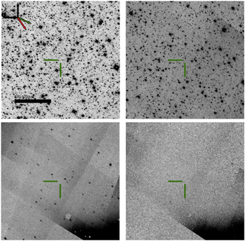
Figure 1. The data for VA (2010 January). Top left is W1, top right is W2, bottom left is W3, and bottom right is W4. Included are an inset of the coordinate axes, where north is up, east is left, the green arrow is the sunward direction, and the red arrow is the direction of heliocentric orbital velocity. Each image is 1800 × 1800 pixels, with a pixel scale of 1''/pixel yielding an image size of 30' × 30'. The expected position of the comet is centered in all the images, and is marked with green bars for clarity. The black bar represents a projected distance of 500,000 km at the comet's location.
Download figure:
Standard image High-resolution image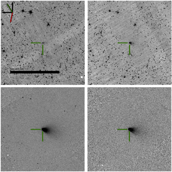
Figure 2. The data for VB (2010 June). The panels and overlays are the same as in Figure 1.
Download figure:
Standard image High-resolution image
Figure 3. The data for VC (2010 July). The panels and overlays are the same as in Figure 1.
Download figure:
Standard image High-resolution imageTable 1. Relevant Information about the Observations
| Visit | Date | Number | rH | Δ | ϕ |
|---|---|---|---|---|---|
| (YYYY-MMM-DD) | of Frames | (au)a | (au)a | (deg)a | |
| VA | 2010 Jan 25 | 12 | 1.66− | 1.25 | −25.08 |
| VB | 2010 Jun 14 | 4 | 1.21+ | 0.66 | 44.33 |
| VC | 2010 Jul 16 | 14 | 1.62+ | 1.17 | 28.22 |
Note.
arH is the heliocentric distance at observation, with – indicating inbound and + indicating outbound; Δ is the observer distance; ϕ is the angular separation of the orbital plane.Download table as: ASCIITypeset image
In order to boost the signal-to-noise of the data, the images for each comet were stacked using Image Co-addition with Optional Resolution Enhancement (ICORE (Masci 2013), formerly AWAIC (Masci & Fowler 2009)). This program co-adds all the frames in which an object was expected to appear, using background matching and outlier rejection to produce a mosaic image. Since the comet is moving relative to the fixed background, the coadded image has the beneficial effect of averaging away most stationary sources such as stars and galaxies where the images overlap. The software uses top-hat area-weighted interpolation to generate an image with a final pixel scale of 1'' per pixel. The center of the image is the predicted comet location based on the comet's ephemeris, and the mosaic is rotated such that equatorial north is up and east is left.
3. Methodology and Results
3.1. Nucleus Size
Since the coma was fainter in VC than in VB, and thus the signal from the nucleus was less obscured, we chose VC to remove the coma and extract the nucleus signal. The coma removal process involves fitting the coma in azimuthal wedges as a function of the angular distance from the central brightness peak (see Lisse et al. 1999, 2009; Fernández et al. 2000, 2013), and has previously been successfully applied to WISE data (Bauer et al. 2011, 2012, 2015). The extracted nucleus signal is then fit to a NEATM, described in more detail in Bauer et al. (2015), yielding a 1σ upper bound on the nucleus diameter of 0.7 km, and a 3σ upper bound of 2.2 km. Due to high residuals, only an upper bound could be calculated. Our nondetection of the comet at its predicted position in VA, less than six months prior to its discovery, yielded a 1σ upper limit on the size of ∼0.8 km in diameter, or a 3σ upper limit of ∼2.4 km. Henceforth in this paper, we will use the upper bound of 2.2 km as the comet's diameter.
3.2. CO+CO2 Production and Active Fraction
A W2 excess above the dust thermal signal was apparent in both VB and VC (see Figure 4). Two strong emission bands from CO (4.67 μm) and CO2 (4.23 μm) reside within the W2 (4.6 μm) bandpass (Bauer et al. 2015). The CO2 band has a fluorescence efficiency approximately 11.6 times stronger than the CO band (see Crovisier & Encrenaz 1983), and so is often assumed to dominate the bandpass, unless it is likely that CO is more than 12 times as abundant as CO2. This may be the case at large heliocentric distances, for example for 29P/Schwassmann-Wachmann 1 (Senay & Jewitt 1994). The photometry of the comet in W2 actually included emission from both gas and dust, and these components must be separated before proceeding with the analysis. As demonstrated in Bauer et al. (2015), the extraction of CO+CO2 excess signal first requires an estimate of the contribution from thermal and reflected light signals in the W2 channel. The dust thermal signal is extrapolated from the thermal signal in the W3 and W4 bands using a Planck-function fit, while the reflected light signal is constrained by the W1 band, as described in Bauer et al. (2011, 2012, 2015).
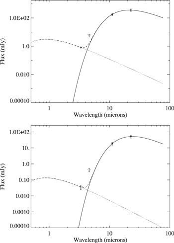
Figure 4. Spectral energy distribution for VB (upper panel) and VC (lower panel). Aperture radii of 11 arcsec were used for the photometry. The W3 and W4 data yielded temperatures of 239 K and 213 K for VB and VC, respectively.
Download figure:
Standard image High-resolution imageThe calculated production rates are shown in Table 2. The excess flux yielded CO2 production rates of 2.7 × 1026 and 1.2 × 1025 molecules s−1 for VB and VC, respectively, assuming CO2 is the dominant species (see Bauer et al. 2015). The corresponding CO production rates are 3.1 × 1027 and 1.4 × 1026 molecules s−1 for VB and VC, respectively. CO2 dissociation lifetimes are ∼5 and 10 days for the comet's heliocentric distances of 1.2 and 1.6 au, respectively, while CO lifetimes are ∼22 and 39 days at these distances (Huebner et al. 1992). It is unlikely, then, that outgassing ceased completely very soon after perihelion, since VB and VC were 52 and 84 days since perihelion, respectively. It is likely, however, that CO or CO2 production dropped dramatically during or soon after VB, since the equivalent production rates were diminished by more than a factor of 20 over the interval of 33 days between visits by the WISE spacecraft's field of view.
Table 2. Coma Photometry
| Visit | Tdust (K) |
 (cm) (cm) |
QCO (molecules s−1) | QCO2 (molecules s−1) |
|---|---|---|---|---|
| VA | 213 | <0.11 | <8 × 1025 | <7 × 1024 |
| VB | 239 | 132 ± 10 | (3.1 ± 0.2) × 1027 | (2.7 ± 0.2) × 1026 |
| VC | 213 | 15 ± 1 | (1.4 ± 0.6) × 1026 | (1.2 ± 0.6) × 1025 |
Download table as: ASCIITypeset image
Given the constraints on nucleus size and CO or CO2 production, we can place constraints on the active area of the nucleus producing these species. From Meech & Svoren (2004, pp. 317–335) it is possible to estimate the gas vaporization rate of a typical cometary nucleus, assuming the case of a surface albedo of a few per cent. CO2 vaporization rates at heliocentric distances of 1.2 and 1.6 au are ∼2.51 × 10²² and 1.25 × 10²² molecules m–2 s−1. Hence, our CO2 production rates correspond to active areas of ∼11,000 m2 and 960 m2, for VB and VC, respectively, or 7 × 10⁻⁴ and 6 × 10⁻⁵ of the fractional area, using the 3σ upper limit of 2.2 km as the comet's diameter. Since the size of the comet is an upper limit, the active fraction we have reported is thus a lower limit. Using the 1σ diameter of 0.7 km yields active fractions of 7 × 10⁻³ and 6 × 10⁻⁴ for VB and VC, respectively. If the activity is primarily driven by CO then the fractional areas would be of the order of 5 × 10⁻³ and 5 × 10⁻⁴ for VB and VC, respectively, for the 3σ upper size limit, and 5 × 10⁻² and 5 × 10⁻³ for the 1σ upper size limit. For comparison, the CO2 active fraction for WISE observations of 67P/Churyumov-Gerasimenko was found to be 1–3 × 10⁻³ (Bauer et al. 2012). We emphasize that the data here do not constrain the H2O production rate, and thus we cannot estimate the active fraction from water ice sublimation, which is likely to be the dominant volatile species at 1.2 and 1.6 au (Meech & Svoren 2004). Due to this limitation, the active fractions of the nucleus derived here should be used only as an upper limit for the CO or CO2 active area, not the total surface area of the comet emitting any volatile species.
3.3. Dust Photometry, Temperature, and Production Rate
Using the techniques described in Bauer et al. (2012, 2015), we can estimate the dust temperature and  values using the W3 and W4 signals. As in Bauer et al. (2012, 2015), we performed thermal fits to the dust coma region, deriving fitted dust temperatures of 239 K for VB and 213 K for VC. These fitted temperatures were used to calculate the factor
  , which is used quantify the amount of dust present in the coma (Lisse 2002; Bauer et al. 2012; Kelley et al. 2013) and is an analog at infrared wavelengths to the quantity
  (A'Hearn et al. 1984) that is frequently derived at visual wavelengths. Table 2 shows the results of the dust temperature and
  modeling. The
  values for VB and VC were 132 ± 10 cm and 15 ± 1 cm, respectively. The
  values derived for C/2010 L5 are somewhat lower than have been reported for other long-period comets (Bauer et al. 2015).
  values for 3.4 μm can be calculated from the W1 flux, and were found to be 43 ± 3 cm for VB. Assuming the same particles contributed to the W1 flux as to the W3 and W4 fluxes, the maximum reflectance would be given by the ratio of the
  and
and  values, multiplied by the emissivity, yielding at most 30% reflectance for the grains. This is an upper limit to the reflectance, since, due to the dependence of scattering efficiency on wavelength, additional smaller particles may contribute more to the flux at shorter wavelengths (Bauer et al. 2008). For VC,
  (1σ detection in W1), implying a grain reflectance ∼0.07 or less.
The rate of dust production can be derived from  fρ values using the formula adapted from Bauer et al. (2008):
where a is the mean grain radius (∼0.03 and 0.1 cm for VB and VC, respectively), ρd is the grain density (∼1 g cm−3), is the average grain emissivity (∼0.9), and vej is the ejection velocity. From Stevenson et al. (2015) we extrapolate vej to be ∼1.1 km s−1 at 1.2 au and ∼0.9 km s−1 at 1.6 au, yielding dust production rates of 23,000 and 2100 kg s−1 for VB and VC, respectively.
3.4. Dynamical Modeling Methods
The morphology of cometary comae, tails, and trails can be used to derive physical properties of their constituent grains such as size distribution, grain speeds, activity history, and dust production rate. Due to the limitations of this particular data set (low spatial resolution, lack of observations over a long time span, short exposures, and mosaicked images causing temporal averaging over the comet's rotation period), we have chosen to employ syndyne–synchrone modeling, based on the Finson–Probstein method (Finson & Probstein 1968) rather than a more complex Monte Carlo modeling technique (e.g., Moreno et al. 2012). While the syndyne–synchrone technique has some serious limitations, in particular the assumption that the particles have zero initial velocity relative to the nucleus, it has been successfully used recently to place useful constraints on the size and emission date of cometary dust (e.g., Kraemer et al. 2005; Reach et al. 2007; Bauer et al. 2012; Stevenson et al. 2012; Jewitt et al. 2013; Kelley et al. 2013; Hainaut et al. 2014; Hui & Jewitt 2015). Further justification for this approximation is given in Section 4.1.
The syndyne–synchrone technique assumes that the motion of cometary dust particles is controlled only by solar gravity and solar radiation pressure, both of which are central forces acting along the Sun–dust particle vector (Finson & Probstein 1968). The particle motion can then be parameterized using the ratio of these two forces, called β:
where

and where Qpr is the scattering efficiency for radiation pressure, c is the speed of light (2.998 × 10⁸ m s−1), Es is the mean total solar luminosity (3.846 × 1026 W), rH is the distance from the Sun, a is the particle radius, G is the universal gravitational constant (6.673 × 10⁻¹¹ N m2 kg−2), Ms is the mass of the Sun (1.989 × 1030 kg), and ρd is the mass density of the particle. Putting Equation (3) and Equation (4) into Equation (2), collecting the constant terms, and converting to cgs units gives
where ρd is now in units of g cm−3, a is the particle radius in cm, and the factor of C = 5.78 × 10⁻⁵ g cm−2 comes from collecting all the constants into a single term (Finson & Probstein 1968).5
Qpr is typically of order unity for particles where  , i.e., particles of order 0.5 μm or larger for most solar radiation (Burns et al. 1979).
β is incorporated into the equation of motion, with the motion of individual particles computed using a numerical integrator (based on the work of Lisse et al. 1998). The comet state vectors (positions, velocities, and accelerations) were calculated using software developed by the NEOWISE team, called "pyPlanetary." The dynamical modeling software takes in a set of β values and comet state vectors (that is, position, velocity, and acceleration vectors for a desired point in time), and integrates the motion of the dust particles over the designated time interval, using the comet's state vectors as the initial conditions for the dust particles. The calculations are carried out in a 3D heliocentric coordinate system, and the final positions of the dust particles are then transformed to the cometocentric coordinate system, projecting the relative positions of the particles onto the observer's (WISE's) plane of sky. The software thus returns a matrix of points that can then be plotted as curves of constant beta (syndynes) or curves of constant particle emission date (synchrones). In this study, we have used β = 3.0 to 0.0001 in steps of half an order of magnitude, and investigated particles that were emitted from five years before the date of observation up to the day before each observation occurred, in one-day intervals.
Each syndyne corresponds to dust with a particular β that was released continuously from some given time ago up to the time of the image. Since the forces on a particle vary with β, the syndynes will tend to fan out in the comet's orbital plane. If the data are well modeled by the syndynes, the curves will span the width of the dust tail when overplotted on the data image. Full Finson–Probstein modeling involves inclusion of the relative velocity of the grains from the comet's surface in the integration, a particle size distribution, and a function to model the number of particles emitted per unit time. With all this, it is possible to create a model image of the comet's coma and tail, which can then be compared to the data (Lisse 2002). For comets where there is no information about the distribution of activity across the surface, an isotropic dust emission model is used (Agarwal et al. 2010), with the initial velocity giving individual β curves a spread of some finite width centered on the zero-velocity syndyne (Lisse 2002). The inclusion of initial isotropic velocity on the dust particles leaving the surface changes the width of the resultant tail, but does not change the overall position. Since this work is concerned with general shape matching, the particles were given no initial velocity relative to the nucleus.
While the dynamical modeling calculations are carried out in fully three-dimensional space, the resultant syndyne–synchrone models fall on the flat plane of the comet's orbit. If the viewing geometry is such that the comet's orbital plane is nearly edge-on to the observer when the data are collected, the models will tend to stack up, causing an ambiguity on the interpretation of the results. In the case of the observations in this paper, the viewing geometry is favorable (see Table 1), and the models are fanned out enough to distinguish between different results.
3.5. Tail-fitting Method
The general method for deriving the results of syndyne–synchrone modeling is to overlay the resulting models on an image, and then select "by eye" the model that most closely matches the morphology of the dust in the image. While we were examining the results of the dynamical models for the comets in the NEOWISE sample, it became clear that this technique was insufficient for a population study, because it is (1) slow and (2) subjective, since independent team members may prefer different models.
In order to mathematically constrain the best-fit syndyne and synchrone of each dust tail, we developed a novel analytical method to collapse a diffuse tail into a set of points, which can then be automatically and systematically compared to the syndynes and synchrones (Kramer 2014). This process allows the best-fit models to be chosen in a much more systematic manner than could be achieved "by eye." The general steps of the method are:
- 1.Split the image into concentric annuli of width s.
- 2.Unwrap the annulus into r–θ space.
- 3.Bin the points into radial bins of width b.
- 4.Fit a Gaussian to the binned points, using the center as the best-fit tail location for that annulus.
- 5.Transform the best-fit tail location back to x–y coordinates.
- 6.Repeat steps 1–5 for a range of annuli (s) and azimuth (b).
- 7.Use a clustering algorithm to remove points that are far from the tail.
- 8.Use a least-squares fitting method to determine separately the best-fit syndyne and synchrone.
Split the image into concentric annuli. Our first task is to split the image into a series of concentric annuli, centered on the comet. For the WISE data, this is somewhat simplified since the ICORE program puts the nucleus at the center of the image (900, 900) during the stacking process. For an annulus of width s, we first omit the region within s pixels of the center, in order to avoid confusion from an extended coma around the nucleus. The remainder of the image is then divided up into concentric annuli out to about halfway to the edge of the image. For the work presented here, we have used annuli of width 20, 30, and 40 pixels, corresponding to 24, 16, and 12 annuli, respectively. See panel B of Figure 5.
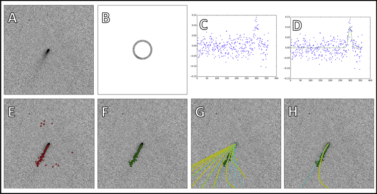
Figure 5. Flow chart of the tail-fitting process. (A) Original image, (B) a selected annulus, (C) unwrapped annulus after binning, (D) Gaussian fit, (E) fitted points superimposed on the image, (F) fitted points with outliers discarded, (G) full set of syndyne–synchrone models, and (H) best-fit syndyne (solid yellow) and synchrone (dashed cyan) overlaid on the image.
Download figure:
Standard image High-resolution imageUnwrap the annulus into r–θ space. Next we unwrap the annulus into r–θ space by first calculating the distance from each pixel location to the location of the nucleus. We then find the angle of each pixel relative to the +x axis.
Bin the points into azimuthal bins of width b. In order to boost the signal-to-noise ratio and thus give a better fit, we then collect the pixels into azimuthal wedges. That is, for a 1° bin, we collect all the pixels with θ between 0° and 1°, adding the value of all the pixels together and dividing by the number of pixels in that azimuthal bin. For the work presented here, we have used azimuthal bins of 1°, 2°, and 3°. See panel C of Figure 5.
Fit a Gaussian to the binned points, using the center as the best-fit tail location for that annulus. In order to aid in the Gaussian fitting, we first subtract the median of all the bins in the annulus. We then (a) fit a Gaussian to these points, saving the results to an array, and (b) create a synthetic Gaussian using the fitted parameters, and subtract that from the points. Steps (a) and (b) are repeated twice more, for a total of three times. This is necessary since occasionally a background star or background noise may be strong enough that the tail signal will be overwhelmed. The best fit to the tail is usually found among the three fitted Gaussians.
We then find the median Gaussian center across the entire set of annuli. If we assume that the comet's tail is the strongest signal in the image, then that Gaussian center value should show up in each set of three values for each annulus. For each annulus, we then select the fitted Gaussian whose center value is closest to the median previously calculated. See panel D of Figure 5.
Transform the best-fit tail location back to x–y coordinates. We next transform the best-fit tail location for each annulus from r–θ space back to x–y coordinates.
Repeat steps 1–5 for a range of s and b. We repeat the process described above for a range of annular widths and radial wedge sizes. Since the comet tails exhibit a wide range of morphologies, there is no one set of s and b that works for all the comets. See panel E of Figure 5.
Use a clustering algorithm to remove points that are far from the tail. In order to boost the strength of the fitted tail and to automatically remove points that are not part of the tail, we employ a clustering algorithm. This algorithm works by first gathering all the fitted tail points (from the entire range of a and b) into a single list. Then the distance between each point and all the others is computed. If there are any points that do not fall within 40 pixels of two other points, those points are discarded. The value of 40 pixels was chosen because this was the width of the widest annulus used in our analysis. See panel F of Figure 5.
Use a least-squares fitting method to determine separately the best-fit syndyne and synchrone. Before comparing the fitted tail points to the models, model points that are far from the center of the image (>2100 pixels from the center in either coordinate) are trimmed to speed up computing time. Next, the synchrones are interpolated, since they only have at most 10 points each, thus making it difficult to compare to the fitted tail points.
The process for finding the best-fit synchrone is similar to finding the best-fit syndyne. In order to compare the fitted tail points to the models, all the points (both fitted and model) are first converted to polar coordinates. Since the tail is roughly radial from the center, using a simple Cartesian comparison of data to model would unfairly penalize points that are far from the nucleus. Then for each fitted tail point, we find the model point for each model that is closest in r, and then find the difference in θ between the fitted tail point and that model point. This is repeated for each synchrone, yielding a list of θ difference values between each model and each fitted tail point. Those θ difference values are squared and added for each synchrone, called "diffsq" for convenience. From the full set of syndyne–synchrone models, shown in panel G of Figure 5, the synchrone with the lowest diffsq is thus chosen as the best-fit synchrone. See panel H of Figure 5.
3.6. Error Estimation
In order to understand the significance of the results that are being presented here, we must estimate the errors on best-fit syndynes and synchrones. We do this by exploiting the fact that the best-fit tail points were chosen using a Gaussian fit: we use the width of the Gaussian (calculated above in Section 3.5) as an estimate of the spread in the tail at a given point. The steps used to estimate the spread in the tail are given here:
- 1.Use the Gaussian width of the best-fit tail points (that is, the standard deviation) as a measure of the error in the fit.
- 2.Subtract (or add) the Gaussian width in pixels for each best-fit tail point from (to) the unwrapped best-fit center location.
- 3.Build up a positive tail and a negative one by repeating this process along the entire length of the fitted tail (see Figure 6, top panel).
- 4.

Figure 6. Example of the process of error estimation for VC. Top panel: positive and negative tail points (circles) and nominal tail points (triangles). Lower left: syndyne models fit to the positive and negative tail points (red dashed) and the nominal tail points (yellow solid). Lower right: synchrone models fit to the positive and negative tail points (red dashed) and the nominal tail points (yellow solid).
Download figure:
Standard image High-resolution image4. Interpretation of the Dust Tail
Before interpreting the results, shown in Table 3 and Figure 7, it is important to recall that synchrones are curves of constant particle emission date, and syndynes are curves of constant β (particle size). Care must be taken when interpreting the results of the tail-fitting method.
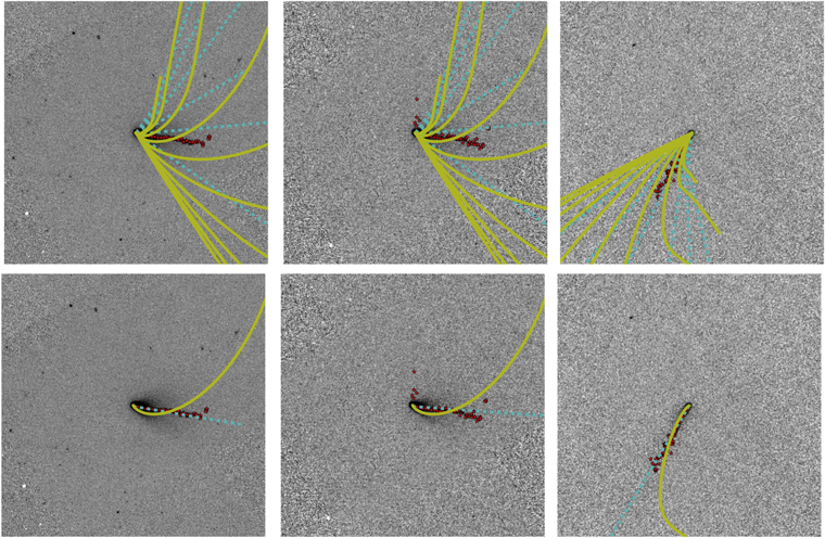
Figure 7. Model syndynes (solid yellow) and synchrones (dashed cyan) overlaid on the images with fitted tail points (red stars). Top row: syndynes range from β = 3.0 to 0.0001 (counterclockwise), and the displayed synchrones are for particles with ages of 30, 60, 90, 180, 365, and 730 days (counterclockwise). The columns are, from left to right, VB W3, VB W4, and VC W4. Bottom row: the best-fit model for each image is displayed. See Table 3 for individual results.
Download figure:
Standard image High-resolution image
Table 3. Results of the Tail-fitting Analysis
| Visit | βa | Synchrone Days | Days Since Perihelion | remdistb |
|---|---|---|---|---|
| VB W4 |

|

|
52 |

|
| VB W3 |

|

|
52 |

|
| VC W4 |

|

|
84 |

|
Notes.
aThe "+" values refer to the positive tail from the error estimation, and are thus a measure of the error bar on the large end of the particles. Similarly, the "−" values refer to the negative tail from the error estimation, and are thus a measure of the error bar on the small end of the particles. Note that the positive error bar on β for VC W4 is the same as the nominal value. This is not a typo. bThe "+" values refer to the error bars on the post-perihelion emission distance, and the "−" values refer to those on the pre-perihelion emission distance.Download table as: ASCIITypeset image
The best-fit synchrone (BFSc) is a measure of the age of the dust in the tail in terms of number of days before the observations took place. For example, if the observations took place on 2010 April 15, and the tail-fitting method yields a BFSc of 180 days, that means that the dust we are seeing was primarily emitted 180 days before the observations took place, or on 2009 October 17. Using the JPL Horizons tool interactively via the web (http://ssd.jpl.nasa.gov/horizons.cgi) or automatically via telnet connection, we can then calculate the heliocentric distance at which the emission occurred by using the calculated emission date. The BFSc is not necessarily a measure of the time all of the dust emission occurred. Rather, it is a measure of the time in the comet's orbit during which the dust emission was strongest. That is, for most comets, dust emission likely occurred both before and after the time (and thus heliocentric distance) indicated by the BFSc, but the BFSc is a useful measure of when the activity was most vigorous. This is especially true since our observations are sensitive to the relatively larger, slower-moving grains.
The best-fit syndyne (BFSd) quantifies the β value that best models the shape of the comet's dust tail. The parameter β must be interpreted with care. To a first-order approximation, it can be used as a proxy for the size of dust particles emitted by the comet by rearranging the terms in Equation (2) to get

which gives the particle size in centimeters when the appropriate values for C, Qpr, ρd, and β are inserted. Thus, for a dust particle with ρd = 0.5 g cm−3 and Qpr = 1, the particle radius in microns is roughly equal to 1/β. The BFSd is a measure of the β value of the brightest part of a comet's tail. That is, the tail contains both particles that are larger and particles that are smaller than suggested by the BFSd, but the BFSd can be used as a proxy for understanding the average particle size in a comet's tail that we can see at WISE's wavelengths.
The top row of Figure 7 shows a range of syndynes and synchrones for VB and VC, and the bottom row shows the best-fit models, summarized in Table 3. In VB, the comet has a wide, nearly conically shaped tail in both W3 and W4. The fitting worked well for both W3 and W4. The BFSc for both W3 and W4 suggested that strong emission occurred at ∼0.79 au, corresponding precisely to the comet's perihelion distance and date (2010 April 23). The BFSd for both W3 and W4 was β = 0.003, suggesting that the particles in the dust tail are on average ∼300 μm in radius.
In VC, the tail was significantly narrower and fainter in both W3 and W4. The W3 fitting did not converge to consistent values, because of some contributions from residual background source emission, but the W4 fitting worked very well. The BFSc for W4 suggested that strong emission occurred at ∼0.79 au, again corresponding precisely to the comet's perihelion distance and date. The BFSd for W4 was β = 0.001, suggesting that the dust particles are on average ∼1 mm in radius.
The BFSd's for each pair of comet images in both wavelengths suggest that the size of the dust particles increased between observations. A natural question to ask is why might the size of the particles increase between observations for C/2010 L5? The time between the pairs of observations was rather short (32 days), and the BFSc suggests that the dust was emitted fairly recently (≲1–3 months before the observations). Additionally, the dust grains were relatively large (β = 0.003–0.001). It is likely that the difference in grain size is due to smaller grains being swept away by solar radiation pressure between observations, or perhaps even disintegrating.
4.1. Effect of Initial Particle Velocity, and Justification for the Zero-velocity Approximation
While Fulle (2004, pp. 565–575) argued that two-dimensional models (i.e., syndyne–synchrone analysis) give unphysical results for calculations of the dust size distribution, here we are using these two-dimensional models to constrain the average size and age of the particles within the tail. We are not trying to measure—and are not claiming that we can measure—the dust size distribution with syndyne–synchrone modeling alone. While measuring the particle size distribution can give useful insights into the nature of the dust, that is not the goal of this work. The modeling of the dust tail presented in this paper is primarily concerned with the average particle size and an estimate of the particle emission date.
Previous versions of the modeling code used in this work have been applied to other cometary dust tails, and the results obtained are consistent with those found by other groups using different modeling techniques. For example, the analysis of size and age of the particles in the dust trail of main belt object P/2012 F5 (Gibbs) in Stevenson et al. (2012) was confirmed by Moreno et al. (2012). The analysis of short-period comet 17P/Holmes in Stevenson et al. (2014) is consistent with results obtained by several other groups including Reach et al. (2010) and Ishiguro et al. (2013). The analysis of the dust trail of 67P/Churyumov-Gerasimenko in Bauer et al. (2012) is consistent with the large particles that have been found by the Rosetta mission (Rotundi et al. 2015), providing further "ground truth" to our modeling techniques. Our analysis of 67P is also consistent with pre-Rosetta results that were obtained by other groups including Agarwal et al. (2007, 2010) and Ishiguro (2008).
A recent paper by Agarwal et al. (2016) gave a quantitative criterion to determine the cases in which the zero-velocity approximation can be used. The criterion involves comparing the effects of velocity from radiation pressure and of particle initial velocity on a particle's energy. If the ejection velocity for a given particle were to have a substantially smaller effect on the particle's energy than acceleration from radiation pressure alone, then the zero-velocity approximation would be valid. In the case of C/2010 L5, the criterion is  m s−1 for particles with β = 0.003 emitted at perihelion, while it is
  m s−1 for particles with β = 0.001. The question is, then, to estimate the initial grain speeds for this comet.
We adopt a relationship for the velocity at which a particle leaves the surface of a comet that is dependent on the particle size and the heliocentric distance in the following way:
where rH is the heliocentric distance at which the particles were emitted and N is taken to be 0.3 (Lisse et al. 1998). We can calculate that particles released at perihelion would have an initial velocity of 18.5 m s−1 if β = 0.003 or 10.7 m s−1 if β = 0.001. Isotropic emission essentially creates a spherical dust shell centered on the nominal dust position that expands over time. We can thus calculate the subtended distance (at the comet's location when the image was taken) to which a dust shell expanding with a particular velocity would grow after a given amount of time. When observed by WISE in 2010 June, the particles with β = 0.003 would have moved from the nominal tail position to a spherical shell with radius ∼83,000 km, projecting to a circle with radius ∼95 arcsec as observed on the image. This is substantially larger than the actual angular distance subtended by the tail, suggesting that the initial particle velocity was substantially lower than estimated from Equation (7). Similarly for the 2010 July data, the particles with β = 0.001 would have moved from the nominal tail position to a spherical shell with radius ∼77,000 km, projecting to a circle with radius ∼66 arcseconds as observed on the image. Thus, Equation (7) overestimates the initial particle velocities in our observations of C/2010 L5.
When comparing the initial velocities predicted by Equation (7) (18.5 m s−1 and 10.7 m s−1 for particles with β = 0.003 and 0.001, respectively) to the criterion from Agarwal et al. (2016) (96.3 m s−1 and 32.1 m s−1 for particles with β = 0.003 and 0.001, respectively), we can see that the predicted velocities are substantially smaller than the zero-velocity criterion. As described in the previous paragraph, due to the spread in the tail, Equation (7) likely overestimates the initial particle velocities. If, for example, we take the initial velocity to be 50% of that predicted by Equation (7), then the spread of the particles in the images would be substantially smaller, but the effect of the initial velocity of a particle on its energy would be even more quickly overwhelmed by that imparted by solar radiation pressure, thereby allowing us to neglect the initial velocity in our analysis of the particle motion.
5. Conclusions
Comet C/2010 L5 (WISE) was observed in three separate epochs, and was detected in the latter two. The analysis presented here suggests that:
- 1.The upper limit of the comet's diameter is 2.2 km.
- 2.The CO2 production rates were 2.7 × 1026 and 1.2 × 1025 molecules s–1 in 2010 June and July, respectively.
- 3.Assuming only CO2 production and a nucleus diameter of 2.2 km, the active fraction of the nucleus is 7 × 10⁻⁴ and 6 × 10⁻⁵ in 2010 June and July, respectively.
- 4.The dust tail seen in the June and July data was formed as a result of strong emission occurring within a few days of the comet's perihelion passage.
- 5.The particles in the dust tail had β values of 0.003 in June and 0.001 in July, suggesting average particle sizes of ∼300 μm and ∼1 mm in radius.
- 6.The dust production rate was ∼23,000 kg s–1 for June and 2100 kg s−1 for July.
Together, these conclusions suggest that C/2010 L5 experienced a significant outburst event when it was close to perihelion. The two separate epochs of dust tail analysis independently suggest a strong emission event close to perihelion. The average size of the dust particles in the dust tail increased between the epochs, suggesting that the dust was primarily released in a short period of time, and the smaller dust particles were quickly swept away by solar radiation pressure, leaving the larger particles behind. The difference in CO2 and dust production rates measured in 2010 June and July is not consistent with "normal" steady-state gas production from a comet at these heliocentric distances, suggesting that much of the detected CO2 and dust was produced in an episodic event.
The tail-fitting technique described in Section 3.5 represents a substantial improvement on previously used syndyne–synchrone modeling. While the fundamentals of the technique presented here are simple, it allows the best-fit model to be derived analytically without any hands-on intervention from the user. It is therefore both faster and more uniform than more interactive methods. C/2010 L5 is an ideal test-case for this technique. The multi-epoch nature of these observations gives us the opportunity to investigate the temporal aspect of the dust properties, and to do a consistency check on our modeling techniques. Future publications will include the application of this method to the entire NEOWISE database of comet dust tails.
This publication makes use of data products from NEOWISE, which is a project of the Jet Propulsion Laboratory/California Institute of Technology, funded by the National Aeronautics and Space Administration. This research has made use of the NASA/IPAC Infrared Science Archive, which is operated by the Jet Propulsion Laboratory, California Institute of Technology, under contract with the National Aeronautics and Space Administration. E.K. gratefully acknowledges funding support from the NASA Postdoctoral Program.
Footnotes
- 5
Note that the value for C is slightly different than that presented in Finson & Probstein (1968), due to differences in the measured value of Es.