


Abstract
SW Sex is a deeply eclipsing cataclysmic variable with an orbital period of 0.1349 days. Based on the new photometric observations together with the data collected in the literature, we find that the orbital period shows a period wiggle from 1980 to 2015, and then decreases severely until 2020, when our observations end. If the oscillation with an amplitude of 0.000973 days and a period of 36.57 yr is due to the presence of a third body, the mass of this component can be determined as M3sini' = 0.014 M⊙. Supposing the companion and the central binary are coplanar, its mass would correspond to a giant planet. However, Applegate's mechanism can also provide enough energy to force such variation and more data will distinguish the reason. The rapid decline of the orbital period at a rate of −4.24 × 10⁻¹⁰ s s−1 in 2015–2020 cannot be attributed to magnetic braking. Also, Applegate's mechanism fails to produce such a fast decrease. It can be explained as the angular momentum loss caused by a strong disk wind, which declares its existence by synchronizing the period decrease with the brightness increase. In addition, the long-term brightness oscillation with an amplitude of 0.6 mag and a timescale of about 9.7 yr is discovered. This is the first it has been detected for nova-like cataclysmic variables (CVs). It will provide valuable information for understanding the disk activity and the evolution of the CVs.
Export citation and abstract BibTeX RIS
1. Introduction
Cataclysmic variables (CVs) are interacting binary systems consisting of a white dwarf and a late-type Roche-lobe-filling red dwarf. Mass is transferred from the companion to the white dwarf via the inner Lagrange point L1, which can form an accretion disk surrounding the primary, and a bright spot appears when the accretion stream from the secondary collides with the disk. Both sources are usually dominant in optical and ultraviolet radiation. Nova-like variables are a subclass of CVs that has never been observed to experience nova or dwarf nova outbursts (Warner 1995). SW Sextantis-type nova-like stars have very high mass-transfer rates and particularly stable accretion disk structures, which maintains the system in a persistent bright state. They are special systems that were first coined by Thorstensen et al. (1991). A number of possible models had proposed to understand their behaviors (Honeycutt et al. 1986; Williams 1989; Hellier & Robinson 1994; Dhillon et al. 1997, 2013), but some mysteries still remain. The orbital period distribution of CVs was found in different surveys (Palomar Green, ROSAT, Edinburgh Cape, and Hamburg Quasar survey) since the beginning of the 21st century, and the SW Sex stars were discovered to habitually accumulate at the upper edge of the period gap (Gänsicke 2005). Most eclipsing nova-like stars with an orbital period between 3 and 4 hr are SW Sex stars. The reason why they inhabit the orbital period range above the gap, however, is still unknown. Schmidtobreick et al. (2012), who provided sufficiently observed data, also indicated that their nonmagnetic samples in this period regime show at least some characteristics of SW Sex, especially the extremely high mass-transfer rates (10−8M⊙ yr−1). According to the standard model of CV evolution, all longer period systems evolved to shorter period systems, driven by angular momentum losses (AMLs). There is a possibility that the SW Sex stars are a distinguished stage in CV evolution, making it especially important to study them (Kjurkchieva et al. 2015).
As the prototype, SW Sex has attracted an abundance of photometric and spectroscopic observational studies. It was discovered as an ultraviolet-excess object in photographic films obtained for the Polomar–Green survey (Green et al. 1986). Green et al. (1982) presented a spectroscopic observation of this target and revealed a high-excitation emission-line spectrum; they suggested that it is a nova-like variable. A follow-up study was done by Penning et al. (1984), who provided evidence to show that the source of flickering is extended over the entire accretion disk. The photometric study shows that the eclipse depth reaches 1.9 mag and the orbital period is 3 hr 14 minutes 18.7 s. The spectrum also shows strong high-excitation lines at optical and UV wavelengths. Honeycutt et al. (1986) and Williams (1989) provided the high-resolution spectroscopic studies and came up with an accretion disk wind and a magnetic accretion stream to explain the single-peaked emission-line profiles, respectively. The phase-dependent absorption features were observed by Honeycutt et al. (1986) and Szkody & Piché (1990), but no model can commit all the phenomena. High speed photometry of the target was described in detail by Ashoka et al. (1994), who attributed the enhanced pre-eclipse hump in a light curve to a bright spot. And the presence of a bright spot is also confirmed by Dhillon et al. (1997).
So far, there is a lack of sufficient effective data analyses on the long-term orbital changes. Studying eclipses of binary stars can reveal evidence of changes in their orbital periods. Boyd (2012) carried out a study of the orbital periods of 18 deeply eclipsing SW Sex stars. The result indicates most of them are consistent with a constant orbital period. Two stars (V363 Aur and BT Mon) show secular period reduction with rates of −6.6 × 10⁻⁸ days yr−1 and −3.3 × 10⁻⁸ days yr−1. Three (SW Sex, LX Ser, and UU Aqr) show possible cyclical variation in their orbital periods. Since the time span of these observations is relatively short, more data is needed to confirm these results. Eclipsing binaries are also very good targets to search for planetary-mass companions orbiting the central systems. By analyzing the O − C variations, some extrasolar planets surrounding CVs have been successfully detected, e.g., DP Leo (Qian et al. 2010), UZ For (Potter et al. 2011), V2051 Oph (Qian et al. 2015), SDSS J143547.87 + 373338.5 (Qian et al. 2016), DV UMa (Han et al. 2017), and DE CVn (Han et al. 2018). In this paper, we will also show the investigation of the secular light variations and discussed the evolutionary state of the systems.
2. Observations and Data
SW Sex was monitored from 2009 April to 2019 March by many telescopes, including the 2.4 m telescope and the Sino-Thai 70 cm telescope in the Lijiang station of Yunnan observatories (YNAOs); the 2.16 m and the 85 cm telescopes at Xinglong Station administered by National Astronomical Observatories, Chinese Academy of Sciences; and the 1.0 m and the 60 cm reflecting telescopes at YNAOs. No filters were used for all observations to improve the temporal resolution. The observed CCD images were reduced by applying the Image Reduction and Analysis Facility (IRAF) software with aperture photometry. The nearby nonvariable comparison star (10h15m18 03, −03°07'19
 33, J2000.0) and check star (10h15m2443, −03°08'2816, J2000.0) were chosen to perform the differential photometry. Most light curves obtained with the above telescopes are shown in Figure 1. Although the light curves have different pre- and post-eclipsing light levels and variable eclipse depths range from 1.6 to 1.9 mag over the past 10 years, the eclipse profiles exhibit symmetrical V shapes. So these profiles with phase widths of 0.06 centering on the mid-eclipse were fitted using a Gaussian function and 18 mid-eclipse times, listed in Table 1, were obtained with their errors determined in a Monte Carlo manner in which the data points are sampled based on their uncertainties and the standard deviation of the mid-eclipse times calculated from all sample sets was taken as its error. Apart from these observations, we also retrieved the American Association of Variable Star Observers (AAVSO) database.6
Considering the accuracy, only the data of V-band (Figure 2) was selected to calculate the eclipse times using the same method as above. All eclipse profiles with phase widths of 0.06 can be fitted well by the Gaussian curve, and some examples of the fitting are displayed in Figure 3. In all 147 new eclipse minima are collected for the study of orbital period variation and are available as supplemental online material.7
33, J2000.0) and check star (10h15m2443, −03°08'2816, J2000.0) were chosen to perform the differential photometry. Most light curves obtained with the above telescopes are shown in Figure 1. Although the light curves have different pre- and post-eclipsing light levels and variable eclipse depths range from 1.6 to 1.9 mag over the past 10 years, the eclipse profiles exhibit symmetrical V shapes. So these profiles with phase widths of 0.06 centering on the mid-eclipse were fitted using a Gaussian function and 18 mid-eclipse times, listed in Table 1, were obtained with their errors determined in a Monte Carlo manner in which the data points are sampled based on their uncertainties and the standard deviation of the mid-eclipse times calculated from all sample sets was taken as its error. Apart from these observations, we also retrieved the American Association of Variable Star Observers (AAVSO) database.6
Considering the accuracy, only the data of V-band (Figure 2) was selected to calculate the eclipse times using the same method as above. All eclipse profiles with phase widths of 0.06 can be fitted well by the Gaussian curve, and some examples of the fitting are displayed in Figure 3. In all 147 new eclipse minima are collected for the study of orbital period variation and are available as supplemental online material.7
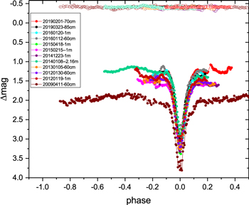
Figure 1. Clean-filter phase-folded light curves of SW Sex obtained with different telescopes. Solid dots represent the magnitude differences between SW Sex and the comparison star, while open circles represent the magnitude differences between the comparison star and the check star.
Download figure:
Standard image High-resolution image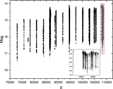
Figure 2. Light curves of SW Sex at V band acquired from the AAVSO database; the observation time spans from 2007 March to 2020 June. A zoom on the newest data is presented in the bottom right-hand panel.
Download figure:
Standard image High-resolution image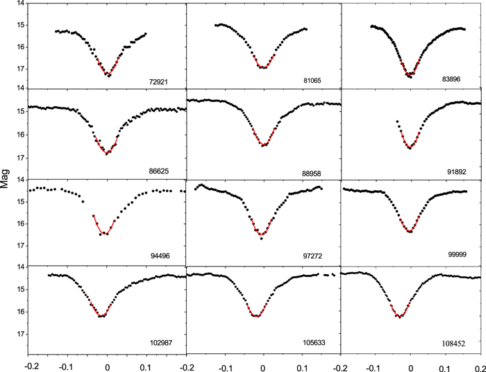
Figure 3. Some examples of the fits for SW Sex using the AAVSO data. The solid circles represent the observations, while the solid lines refer to Gaussian fits of the eclipse profiles with phase widths of 0.06. For clarity, the eclipsing profiles were plotted on the same scale along the phase and mag.
Download figure:
Standard image High-resolution imageTable 1. Our Mid-eclipse Times of SW Sex
| Date | Min.(HJD) | Min.(BJD) | Error | Cycle | O − C(days) | Telescope |
|---|---|---|---|---|---|---|
| 2009 Apr 11 | 2454933.13097 | 2454933.13176 | 0.00015 | 78506 | 0.00043 | 60 cm |
| 2011 Apr 3 | 2455655.05174 | 2455655.05253 | 0.00010 | 83856 | 0.00028 | 85 cm |
| 2012 Jan 19 | 2455946.24897 | 2455946.24975 | 0.00009 | 86014 | 0.00024 | 1 m |
| 2012 Jan 19 | 2455946.24899 | 2455946.24977 | 0.00010 | 86014 | 0.00026 | 60 cm |
| 2012 Jan 30 | 2455957.31347 | 2455957.31425 | 0.00008 | 86096 | −0.00022 | 60 cm |
| 2012 Mar 29 | 2456016.14684 | 2456016.14762 | 0.00007 | 86532 | −0.00031 | 85 cm |
| 2012 May 16 | 2456064.04999 | 2456064.05077 | 0.00004 | 86887 | −0.00047 | 2.4 m |
| 2013 Jan 5 | 2456298.30302 | 2456298.30380 | 0.00009 | 88623 | −0.00023 | 60 cm |
| 2014 Jan 8 | 2456666.41564 | 2456666.41641 | 0.00018 | 91351 | 0.00018 | 2.16 m |
| 2014 Dec 23 | 2457015.36613 | 2457015.36689 | 0.00005 | 93937 | −0.00028 | 1 m |
| 2015 Feb 15 | 2457069.20685 | 2457069.20761 | 0.00015 | 94336 | −0.00013 | 1 m |
| 2015 Feb 24 | 2457078.24743 | 2457078.24819 | 0.00008 | 94403 | −0.00031 | 1 m |
| 2015 Apr 18 | 2457131.14377 | 2457131.14453 | 0.00009 | 94795 | 0.00014 | 1 m |
| 2016 Jan 12 | 2457400.34554 | 2457400.34631 | 0.00015 | 96790 | −0.00037 | 60 cm |
| 2016 Jan 20 | 2457408.30718 | 2457408.30795 | 0.00004 | 96849 | −0.00010 | 1 m |
| 2016 Mar 8 | 2457456.21007 | 2457456.21084 | 0.00004 | 97204 | −0.00037 | 1 m |
| 2019 Feb 1 | 2458516.42011 | 2458516.42093 | 0.00004 | 105061 | −0.00200 | 70 cm |
| 2019 Mar 25 | 2458566.07759 | 2458566.07842 | 0.00003 | 105429 | −0.00188 | 85 cm |
Download table as: ASCIITypeset image
In addition, some light curves are featured by the flickerings, which means the process of mass-transfer from the red star to the white dwarf is turbulent. In order to study the periodicity of the flickerings, all the light curves were dropped off the eclipses and each light curve was subjected to the period searching for the signal peak longer than 1 hr using the Lomb–Scargle method (Lomb 1976; Scargle 1982). Considering the length of each data set, we think this signal was related to the tread of the light curve rather than the flickering and was subtracted from the data, and this process was operated 3 times at most, then the periodical signal of less than 1 hr was searched for from the resultant data. At last only three light curves from different epochs (Figure 4) show quasi-periodic behavior with the peak periods of 0.6341 hr, 0.4850 hr, and 0.3973 hr, respectively. These flickerings have amplitudes of several hundredths of one mag, and exist not only in a high state, but also in a low state. Due to the limitation of the quality of observation data and incomplete phase coverage of some light curves, the regularity of their occurrence is difficult to summarize.
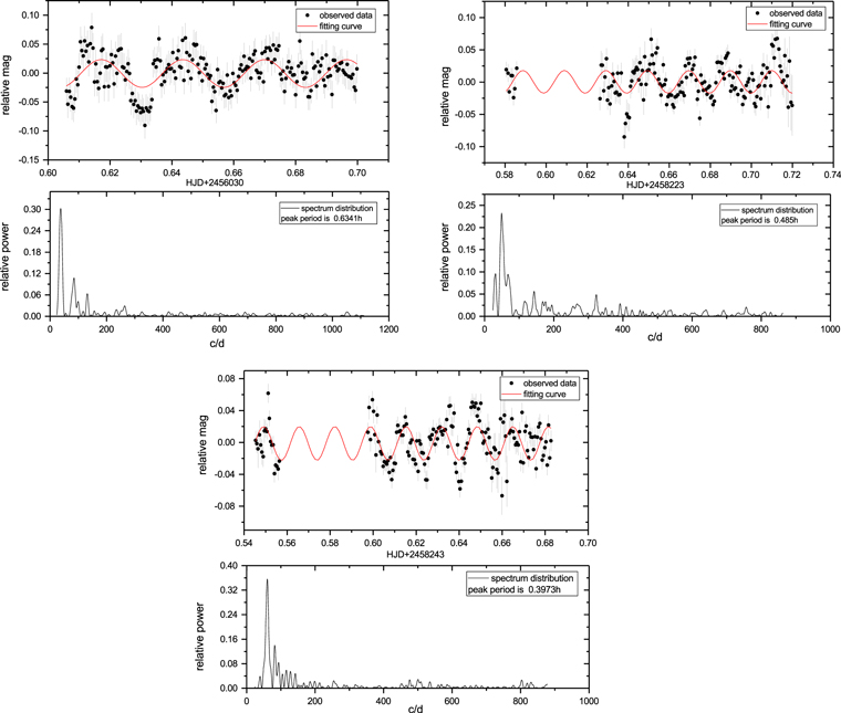
Figure 4. Periodicity of the flickerings. Three panels show the observations at different times and their corresponding power spectra. The eclipsing intervals were removed from the raw data, and the trends higher than 1 hr are eliminated. The red lines are sine fittings with periods of 38 minutes, 29 minutes, and 24 minutes, respectively.
Download figure:
Standard image High-resolution image3. Analysis and Results
3.1. Orbital Period Changes
The observed eclipse minima of SW Sex have been presented previously (e.g., Penning et al. 1984; Ashoka et al. 1994; Dhillon et al. 1997; Groot et al. 2001; Boyd 2012). Based on the published data (Penning et al. 1984), Ashoka et al. (1994) deduced that the orbital period increases in the rate of 2.2 × 10⁻¹¹ s s−1. Given that there are only a few eclipse minima and most of them cluster, the investigation of longer-term observations is urgently required. Coupled with all archive mid-eclipse times, collected from the literature and the O − C Gateway database,8 there are 190 eclipse minima in total within the time span of about 40 yr. In order to eliminate the Earth's motion and light-travel time effects, times for all the observations have been converted to Barycentric Julian Day (BJD) in Barycentric Dynamical Time (Eastman et al. 2010). These minima can be used to derive a more accurate linear ephemeris

We assigned different weights to these eclipse times during the fitting process because of their different uncertainties, where the weights were inversely proportional to the rms errors. The residues of the linear fit (denoted as O − C) are plotted in the upper panel of Figure 5, which shows a possible cyclic oscillation. Orbital period oscillation is often attributed to the mechanism of Applegate (1992) or/and the presence of a third body orbiting the binary. The model involving the third body urges at least a brown dwarf along in a highly eccentric orbit (∼0.8) and indicates the presence of a forth body, which complicates the system and is beyond the prediction of the data (overfitting), and thus is not reliable. Considering the secular light-curve variation, we find that the O − C values fall more sharply after 95,000 runs synchronize with reaching a higher state (see Figure 2), so the O − C data is divided into two parts by the boundary (95,000 runs). The first part is modeled by an cyclic oscillation

and the other one by a quadratic function

where β is the coefficient of the quadratic term. As shown in the upper panel of Figure 5, the dark solid line denotes the best fitting of the oscillation, and the red solid line represents the quadratic fit. The residuals are shown in the bottom panel; there is no other variation that can be traced suggesting that these equations could model the O − C data enough. The fitting parameters are listed in Table 2.
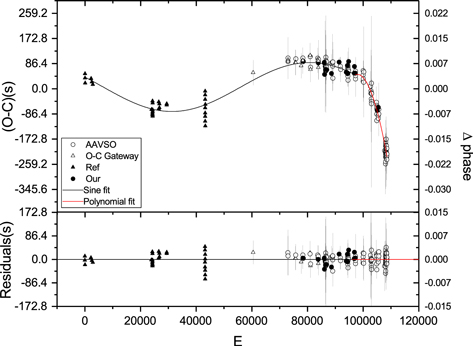
Figure 5. O − C values are displayed in the upper panel. The black solid line refers to the best-fitting sinusoidal curve, and the red line denotes the best quadratic fit. After all changes are removed, the residuals are shown in the lower panel. The solid triangles denote the published times, solid circles denote our new eclipsing times, and open circles and open triangles refer to the data from AAVSO and O − C Gateway databases, respectively.
Download figure:
Standard image High-resolution imageTable 2. Parameters of the Orbital Period Changes in SW Sex
| Parameters | Sine Fitting: (O − C)1 |
|---|---|
Revised epoch,  (days) (days) |
7.04(±2.67) 
|
| Semiamplitude, K(days) | 0.000973 (±0.000031) |
Orbital period, P3 =  (yr) (yr) |
36.57 (±1.16) |
Orbital phase, 
|
−203.66 (±3.69) |
| Parameters | Quadratic fitting: (O − C)2 |
Revised epoch,  (days) (days) |
−0.27342(±0.02888) |
Revised period, 
|
5.60(±0.56) 
|
| Rate of period decrease, 2β (days/cycle) | −5.72(±0.53) 
|
Download table as: ASCIITypeset image
3.2. Secular Light-curve Variations
SW Sex has been observed by DASCH (Digital Access to a Sky Century at Harvard). DASCH is a project to digitize and analyze the collection of 500,000 glass photographic plates held at the Harvard College Observatory. The plates were exposed from 1880 to 1990 (Laycock et al. 2010). It covers a much longer historical period, albeit at a lower sensitivity; however, we are only able to provide the long-term photometric behavior. The data of the object from DASCH is shown in Figure 6 ranging from JD2415000–JD2447000, and the distribution of the data is sparse and random. Considering that the occultation interval, approximately 40 minutes, only occupies 20% of the whole orbital period, it is highly possible that most data corresponds to the out-of-eclipse magnitude of the system. We supplement the latest data with wide band V to JD2459000. Since AAVSO data are in V band, while DASCH magnitudes are in B band, their mean brightness is not at the same level. Given that most of the radiation comes from the accretion disk and the effective temperature of the disk is about 14,000(±6000) K (Rutten et al. 1992), we should subtract about 0.15(±0.09) mag in AAVSO V mag to the DASCH B mag (Cox 2000).
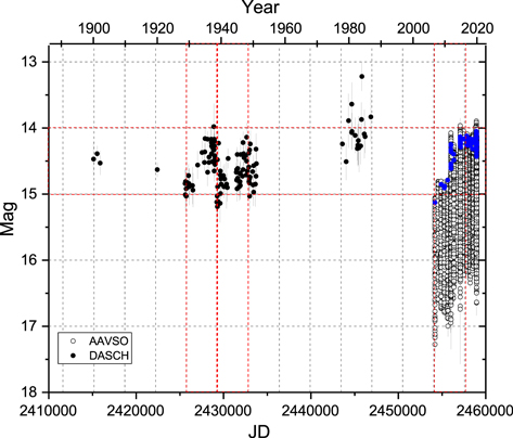
Figure 6. Photometric data of SW Sex from DASCH and AAVSO. The black solid circles are the data from DASCH and the open circles from AAVSO with the blue dots denoting the mean out-of-eclipse brightness. The horizontal red dotted lines limit the brightness variation. The vertical grid lines space 3535 days.
Download figure:
Standard image High-resolution imageAs shown in Figure 6, the black dots represent the data from DASCH. The open circles are from the AAVSO database, and the light curves have been overlaid by the mean mag of the out-of-eclipse, which are donated by blue circles. We have subtract 0.15 mag in the plot without considering interstellar extinction E(B − V) = 0. The brightness variation of the system in the figure indicates that it wanders irregularly on a characteristic timescale of several years. DASCH data show two gradual increases and the AAVSO data show one. The DASCH data exhibit that the brightness quickly decayed, in less than 300 days, and then was eager to recover. The AAVSO data also shows that the brightness of the system increased, but after that, the luminosity had been stagnating for several years. These three enhancements show the same amplitude variations, about 0.6 mag, in general. We take 3535 days (about 9.7 yr) as a mag-changing cycle, which are split by the black dashed vertical lines shown in Figure 6, and the luminosity increase happens to occur within this time interval. If we boldly assume that the magnitude increases linearly and the rising time interval is about 9.7 yr, the brightness will decay and reach the peak magnitude again in the next decade, repeating the pattern that occurred before. However, the system exhibits the highest luminosity and currently shows stagnation. The newest rich data show that these oscillations saturate at a low amplitude. The luminosity is expected to be dropped rapidly in the near future. So it is necessary to be monitored continuously in the future to sum up the characteristics of the possible 10 yr period state changes and find out the mechanism behind it.
4. Discussions
4.1. The Mechanism for the Possible Cyclic Orbital Period Variation
Based on the investigation of the (O − C) diagram, we found the orbital period of SW Sex undergoes a period oscillation with a timescale of about 36 yr. The period wiggle in binary systems is generally caused by Applegate's mechanism (Applegate 1992) or by the light-travel time effect due to the presence of a third companion (e.g., Li et al. 2017; Fang et al. 2019; Zhu et al. 2019). According to the Applegate's mechanism, the period variations are caused by the magnetic activity of the secondary star, which drives the redistribution of angular momentum in the interior of the star. From the semiamplitude (K) and the modulation period (Pmod) of the orbital period oscillation, using the equation

the fractional period change Δ P/P was determined to be 4.57 × 10⁻⁷. Penning et al. (1984) derived the masses of the primary and the secondary stars as M1 = 0.58 ± 0.20 M⊙ and M2 = 0.33 ± 0.06 M⊙, respectively, and the orbital inclination i = 79° ± 1° from the dynamical analysis of the system, while Dhillon et al. (1997) doubted their method and constrained the component masses to M1 ∼ 0.3–0.7 M⊙, M2 < 0.3 M⊙, and i > 75°. Assuming the typical mass of the primary as  and that of the secondary as
  , the radius of the secondary star is
  (McAllister et al. 2019) and the binary separation is
  from Kepler's law. According to

we can calculate the variation of the quadrupole moment of the secondary star to be  . The secondary star may approach the full convective state so it can be modeled using the Lane–Emden equation for an n = 1.5 polytrope. We followed the same method of Brinkworth et al. (2006) to split the whole star into an inner core and an outer shell, and the required energy
  to diver the variation of the quadrupole moment
  can be determined for a different range of the shell mass, as displayed in the right panel of Figure 7. The luminosity of the secondary star is
  , which, for
  , gives the energy available over the 36.57 yr as
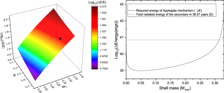
  . This value, indicated in the right panel of Figure 7, succeeds in supplying enough energy to modulate the orbital period. A plot of the ratio of the value of minimum energy required to drive the Applegate's mechanism over the energy supplied in 36.57 yr versus the mass of two components is shown in the left panel of Figure 7. Applegate's mechanism can be responsible for the period oscillation if the value of
  (ΔEmin/E) is greater than 0. The results indicate that Applegate's mechanism cannot be excluded to interpret the period variation.
Figure 7.
 (ΔEmin/E) versus different sets of masses of primary and secondary stars. The mass of the white dwarf was constrained to M1 ∼ 0.3–0.7 M⊙, and the secondary star's was limited to M2 ∼ 0.2–0.33 M⊙. The right panel shows a plot of the required energy versus different shell mass in the case of M1 = 0.6 M⊙ and M2 = 0.3 M⊙, which is represented with a black dot in the left panel.
Download figure:
Standard image High-resolution image
Another plausible explanation is the light-travel time effect of a third body. Assuming that the third body is coplanar with the central host systems (i.e.,  = i = 79°), the minimum mass of the third companion is estimated to be M3sini' = 0.014 M⊙ with a separation of 10.52 au, which indicates that it may be a giant planet. Parameters of the third body are shown in Table 3, the calculation is based on M1 = 0.6 ± 0.2 M⊙, M2 = 0.3 ± 0.1 M⊙.
Table 3. Parameters for the Third Body of Light-travel Time Effects in SW Sex
| Parameters | Values and Error |
|---|---|
Eccentricity ( ) ) |
0.0 |
| Period (P3) | 36.57 (±1.16) yr |
| Amplitude (K3) | 0.000973 (±0.000031) day |
 sin sin
|
0.17 (±0.01) au |
| f(m) | 3.58(±0.32) × 10−6 M⊙ |

|
0.014 (±0.002) M⊙ |
| a3 | 10.52 (±3.97) au |
Download table as: ASCIITypeset image
On the basis of the current data, both mechanisms can explain the variation of the orbital period and the time span of the observations is too short compared to the timescale of the period oscillation, so further monitoring of SW Sex is necessary.
4.2. The Interpretations for the Orbital Period Decrease
As shown in Figure 5, the O − C curve falls sharply following 95,000 runs, which is beyond the prediction of the theoretical sine-wave (O − C)1. Thus, a quadratic curve (O − C)2 is applied to describe it. The binary shrinks its orbits due to an AML from the system. For a close star with the orbital period of 3.24 hr (≥3 hr), the orbital angular momentum of the system is taken away by the magnetic braking (MB) mainly due to the magnetized stellar wind (Verbunt & Zwaan 1981). Although gravitational radiation (GR) can also work at the same time in the system, it is relatively much smaller (Paczynski & Sienkiewicz 1981). Rappaport et al. (1983) proposed a formula to calculate the orbital period decrease due to MB,
where γ is the MB index in a range from 0 to 4. The standard MB, γ = 4, predicts the orbital period decrease of  MB = −5.44 × 10⁻¹² s s−1, it is about two orders of magnitude smaller than the period decay listed in Table 2. Even the highest decreasing
  MB = −2.41 × 10⁻¹⁰ s s−1 in the framework of the MB, γ = 0, fails to explain such an observed period decrease.
Given that the CV evolution is derived partially by AMLs via mass loss from the disk (King 1995) and SW Sex has a very high mass-accretion rate, we think the only factor leading to the fast period decrease is the wind emanating from the accretion disk. Comparison between Figure 2 and Figure 5 shows that the fast period decrease is accompanied by the luminosity maximum. When the system reaches the highest luminosity, the strong radiation induces a thick disk wind that can prevent the accretions onto the disk and takes away a lot of angular momentum from the system. The latest data of the brightness of the system shows a small amplitude oscillation (see Figure 2), and this phenomenon may also be evidence for the wind-driven instability in the accretion disk. Such a situation was originally put forward by Begelman et al. (1983) and Shields et al. (1986). To assess the role of the disk winds, they defined  and
and  as the wind mass-loss rate and mass-accretion rate onto an accretor, respectively. The ratio C =
  /
/ measures the efficiency of wind driving due to the accretion power and indicates how strongly the wind is coupled to the latter. For a large value of C, a small increase in
  and hence luminosity can induce an increase in
  , which is large compared to
  . If the resultant
  +
+  is larger than the mass input rate from the secondary star, the disk will be depleted. After a delay, both
  and
and  will eventually be reduced. A reduction in
  in turn will cause the disk to be replenished so that
  and the luminosity will once again be increased. We now prove observational evidence of the wind, which takes away angular momentum in the form of mass loss from the disk's surface.
5. Summary
Using the observed times of light minima, we found that the orbital period showed a possible cyclic wiggle from 1980 to 2015, then decreased severely from 2015 to 2020. The oscillation with an amplitude of 0.000973 days and a period of 36.57 yr may be due to the presence of a giant planet or the Applegate's mechanism. While the period decrease within the recent 5 yr is too fast to be produced by AML via MB, suggesting that there could be an additional AML mechanism. During these 5 yr, the system maintained the highest brightness, which indicates that the strong radiation may trigger the disk wind that severely takes away angular momentum, then leads a period in which the system falls faster than expected.
The light curves of SW Sex present flickering in periods of around half an hour, which has been reported before. Such behaviors that survive in the lower brightness state as well as the higher state may indicate that the main source is the hot spot due to unstable accretion.
The DASCH data and the AAVSO data reveal that SW Sex experienced a series of state changes in the pattern of a slow increasing about 0.6 mag in about 9.7 yr following a fast decrease to the low state in less than 300 days. We believe that this kind of long-term variation exists not only in SW Sex, but also in other nova-like stars, although they have not been discovered yet due to their short history of observations. As the prototype of this kind of CV, SW Sex was first discovered to have a maverick behavior, for which the disk activities may be responsible. Thus SW Sex is a very interesting system and is an important astrophysical laboratory to study disk activities.
This work is supported by the National Natural Science Foundation of China (Nos. 11933008 and 11803083). New data presented here were observed with the 60 cm, 1 m, and 2.4 m telescopes and Sino-Thai 70 cm telescope at the Yunnan Observatories; the 85 cm and 2.16 m telescopes in Xinglong Observation base in China. We acknowledge the support of the staff of the Xinglong 2.16 m and 85 cm telescope. This work was partially supported by the Open Project Program of the Key Laboratory of Optical Astronomy, National Astronomical Observatories, Chinese Academy of Sciences. We appreciate the observers from around the world for the contributions of the AAVSO data. And we are very grateful to the DASCH project designed to open the window on variability studies and provided early photographic data for SW Sex. Finally we thank the anonymous referees for a very useful review.