


Abstract
We report individual dynamical masses for the brown dwarfs ε Indi B and C, which have spectral types of T1.5 and T6, respectively, measured from astrometric orbit mapping. Our measurements are based on a joint analysis of astrometric data from the Carnegie Astrometric Planet Search and the Cerro Tololo Inter-American Observatory Parallax Investigation, as well as archival high-resolution imaging, and use a Markov chain Monte Carlo method. We find dynamical masses of 75.0 ± 0.82 MJup for the T1.5 B component and 70.1 ± 0.68 MJup for the T6 C component. These masses are surprisingly high for such cool objects and challenge our understanding of substellar structure and evolution. We discuss several evolutionary scenarios proposed in the literature and find that while none of them can provide conclusive explanations for the high substellar masses, evolutionary models incorporating lower atmospheric opacities come closer to approximating our results. We discuss the details of our astrometric model, its algorithm implementation, and how we determine parameter values via Markov chain Monte Carlo Bayesian inference.
Export citation and abstract BibTeX RIS
1. Introduction
The ε Indi system (GJ 845, LHS 67) is a nearby triple system, and its B and C components are among the T dwarfs closest to our solar system. It is a hierarchical system comprising a K5V primary widely separated from a brown dwarf binary of spectral types T1.5 and T6 for which we find an 11.4 yr orbit. Some previously known properties of the system are listed in Table 1. The brown dwarf component was first announced by Scholz et al. (2003), who established common proper motion to ε Indi A at a projected separation of 402 3. The B component was soon thereafter resolved as a close binary with a projected separation of ∼07 in VLT/NACO observations by McCaughrean et al. (2004) and independently by Volk et al. (2003) on Gemini South. Kasper et al. (2009) and King et al. (2010) independently assigned spectral types T1.5 and T6 for the B and C components. Both studies note slightly subsolar metallicity. We adopt [Fe/H] = −0.13 ± 0.02 based on a weighted mean of literature values for the A component listed in the PASTEL Catalogue (Soubiran et al. 2016).
Table 1. Previously Known Properties of the ε Indi System
| Property | A | B | C | Referencesa |
|---|---|---|---|---|
| Spectral type | K5V | T1.5 | T6 | A: 1; B, C: 2, 3 |
| Parallax (mas) | 276.06 ± 0.28 | ⋯ | ⋯ | 4 |
| Distance (pc) | 3.622 ± 0.004 | ⋯ | ⋯ | 4 |
| μα (mas yr−1) | 3960.93 ± 0.24 | ⋯ | ⋯ | 4 |
| μδ (mas yr−1) | −2539.23 ± 0.17 | ⋯ | ⋯ | 4 |
| Separation (c. 2004) | 4023 |
07 |
07 |
5 |
| [Fe/H] | −0.13 ± 0.02 | ⋯ | ⋯ | 6 |
| V | 4.68 | 24.12 ± 0.03 | ≥26.6 | A: 1; B, C: 3 |
| R | ⋯ | 20.65 ± 0.01 | 22.35 ± 0.02 | 3 |
| I | ⋯ | 17.15 ± 0.02 | 18.91 ± 0.02 | 3 |
| z | ⋯ | 15.07 ± 0.02 | 16.53 ± 0.02 | 3 |
| J | 2.89 ± 0.29 | 12.20 ± 0.03 | 12.96 ± 0.03 | A: 7; B, C: 3 |
| H | 2.35 ± 0.21 | 11.60 ± 0.02 | 13.40 ± 0.03 | A: 7; B, C: 3 |
| K | 2.24 ± 0.24 | 11.42 ± 0.02 | 13.64 ± 0.02 | A: 7; B, C: 3 |
Note.
a(1) Evans et al. (1957); (2) Kasper et al. (2009); (3) King et al. (2010); (4) van Leeuwen (2007); (5) Scholz et al. (2003); (6) Soubiran et al. (2016 and references therein); (7) Cutri et al. (2003).Download table as: ASCIITypeset image
Our understanding of substellar structure and evolution is still incomplete in several aspects. There are still large discrepancies among the predictions of evolutionary models and the properties of both individual objects and observed populations (e.g., Dieterich et al. 2014). The atmospheres of these cool objects are difficult to model due to molecule and cloud formation, leading to a poor understanding of overall opacities, which in turn affects the rate of cooling. Different assumptions regarding atmospheric opacities have led to different evolutionary models arriving at significantly different evolutionary rates, as well as different fundamental properties for objects at the stellar–substellar boundary (Section 5). It has also been suggested that small changes in metallicity and cloud parameters, which in stellar theory are considered secondary properties, may play disproportionately large roles in the structure and evolution of substellar objects (Burrows et al. 2011), thus further complicating attempts at a general characterization. Our theoretical understanding must now be constrained by observations of brown dwarfs amenable to extensive characterizations that yield precise dynamical masses, as well as spectrophotometric properties such as metallicities and spectral energy distributions. Significant progress has been made recently with the publication of a large collection of substellar dynamical masses (e.g., Konopacky et al. 2010; Dupuy & Liu 2012; Dupuy & Kraus 2013; Dupuy & Liu 2017; Bowler et al. 2018). However, most binary substellar systems amenable to dynamical mass determinations in reasonable timescales have very small projected separations that make a thorough spectrophotometric characterization of the individual components difficult. Even when individual spectra can be obtained, our poor understanding of how spectral features vary with metallicity in these cool atmospheres hinders the comparison of different systems.
The ε Indi system's proximity to Earth (3.62 pc), its hierarchical nature with a well-known primary component, and the relatively short period of the BC component make this system an ideal benchmark for the study of substellar structure and evolution. In this paper, we determine dynamical masses for ε Indi B and C by solving the system's complete astrometric motion. We do so by measuring the motion of the unresolved B–C system's photocenter using data from two separate observing programs and then using high-resolution adaptive optics images to scale the photocenter's orbit to the individual barycentric orbits of the B and C components. We discuss our observations in Section 2, our astrometric model in Section 3, and results in Section 4. We conclude with a discussion of how the dynamical masses we report constrain substellar models, with particular emphasis on the stellar–substellar boundary in Sections 5 and 6. Appendix A describes the Markov chain Monte Carlo (MCMC) algorithm and its implementation in detail and provides instructions for downloading and using it. Appendix B provides a detailed example of deriving individual dynamical masses from the photocenter's orbit.
2. Observations
The complete characterization of the motion of an unresolved astrometric binary system requires observations in which the motion of the system's photocenter is measured with respect to the background of distant stars, as well as at least one epoch of resolved imaging (van de Kamp 1968; McCarthy et al. 1991). The photocenter is defined as the centroid of the point-spread function of the combined light from both components, and its location lies along the separation vector between the two components. The precise location of the photocenter along the separation vector is determined by the observed flux ratio of the primary to the secondary component, which is in turn a function of the components' intrinsic spectral energy distribution and the photometric filter used to perform the observations. The observed astrometric motions are the motions of the photocenter about the system's barycenter. These motions are not necessarily equivalent to the motion of the physical components. For a given binary star system, the mass ratio and flux ratio will generally not be the same, thus causing the photocenter and barycenter to lie along different points in the system's separation vector. The photocenter thus traces an orbit about the barycenter that has the same orientation but is smaller than the orbits traced by either component about each other or the barycenter. We discuss the scaling of these orbits and how they relate to dynamical masses in Section 4.1 and Appendix B.
Once the trigonometric parallax motion, proper motion, and orbital motion of the photocenter are deconvolved (Section 3), the flux ratio and separation obtained from a resolved image allow the scaling of the photocenter's orbit to the physical orbits of the primary and secondary components around the system's barycenter, and thus the determination of individual dynamical masses via Kepler's third law. We combined astrometric observations from the Carnegie Astrometric Planet Search (CAPS; Boss et al. 2009; Anglada-Escudé et al. 2012; Weinberger et al. 2016) and the Cerro Tololo Inter-American Observatory Parallax Investigation (CTIOPI; Jao et al. 2005; Henry et al. 2006) to map the photocenter's orbit, parallax, and proper motion. We then used archival high-resolution images taken with the Naos-Conica (NACO) imager on the Very Large Telescope UT4 (VLT/NACO) adaptive optics system to determine the scale factor between the photocentric orbit and the physical orbit. We now discuss these data sets individually.
2.1. CTIOPI Observations
The CTIOPI is a large astrometric program that began in 1999 on the CTIO/SMARTS10 Consortium 0.9 m telescope. The details of the observing procedures and data reduction are discussed in Jao et al. (2005). Between 2004 and 2016, ε Indi BC was observed on 33 nights. Typically, five exposures of 300 s each were taken during each epoch, always in the Kron−Cousins I band. Exposures were usually taken within half an hour of meridian transit to minimize differential color refraction. A single image taken with good seeing, and a low hour angle was selected as the "trail frame" and compared to the 2MASS catalog (Skrutskie et al. 2006) to determine plate rotation and scale. The pixel coordinates of 10 reference stars were then used to create coordinate transformations linking each individual exposure to the reference frame established in the trail frame. Table 2 lists the displacement of ε Indi BC's photocenter with respect to the first epoch of observation. The uncertainties correspond to the standard deviation of the several individual exposures taken during an epoch.
Table 2. Astrometric Observations
| Night | Program | Jul. Date | α Displacementa,b | σα | δ Displacementa | σδ | pαc | pδc |
|---|---|---|---|---|---|---|---|---|
| (mas) | (mas) | (mas) | (mas) | |||||
| 2004 Jul 30 | CTIOPI | 2453216.77 | −1.55d | 3.40 | −4.36d | 3.81 | 0.348 | −0.578 |
| 2004 Aug 07 | CTIOPI | 2453224.74 | 49.13 | 6.08 | −65.45 | 1.93 | 0.227 | −0.638 |
| 2004 Sep 26 | CTIOPI | 2453274.61 | 389.74 | 8.48 | −434.68 | 7.60 | −0.531 | −0.726 |
| 2005 Jul 26 | CTIOPI | 2453577.77 | 3944.09 | 3.98 | −2451.49 | 5.92 | 0.408 | −0.541 |
| 2006 May 18 | CTIOPI | 2453873.91 | 7330.16 | 3.95 | −4247.16 | 3.55 | 0.943 | 0.267 |
| 2006 Jul 05 | CTIOPI | 2453921.81 | 7785.40 | 3.10 | −4751.86 | 5.02 | 0.679 | −0.322 |
| 2007 Jul 26 | CTIOPI | 2454307.82 | 11909.36 | 6.00e | −7472.15 | 6.00e | 0.413 | −0.534 |
| 2007 Aug 08 | CTIOPI | 2454320.78 | 12002.87 | 6.00e | −7595.21 | 6.00e | 0.219 | −0.637 |
| 2007 Oct 26 | CTIOPI | 2454399.52 | 12605.38 | 6.00e | −8123.54 | 6.00e | −0.836 | −0.535 |
| 2009 Jul 30 | CTIOPI | 2455042.68 | 20045.24 | 1.12 | −12700.78 | 1.88 | 0.353 | −0.569 |
| 2010 Jul 31 | CTIOPI | 2455408.81 | 24017.54 | 0.72 | −15296.33 | 10.54 | 0.342 | −0.576 |
| 2010 Sep 29 | CTIOPI | 2455468.58 | 24432.31 | 4.04 | −15751.05 | 2.68 | −0.561 | −0.711 |
| 2011 Jul 01 | CTIOPI | 2455743.83 | 27741.27 | 0.78 | −17493.49 | 2.76 | 0.731 | −0.268 |
| 2011 Sep 23 | CTIOPI | 2455827.62 | 28303.49 | 6.13 | −18174.35 | 12.46 | −0.477 | −0.733 |
| 2011 Oct 07 | CTIOPI | 2455841.60 | 28403.17 | 0.96 | −18261.94 | 2.82 | −0.653 | −0.674 |
| 2012 Jul 05 | CTIOPI | 2456113.82 | 31702.14 | 5.46 | −19990.99 | 6.34 | 0.681 | −0.324 |
| 2012 Sep 12 | CTIOPI | 2456182.65 | 32155.83 | 1.77 | −20569.75 | 6.44 | −0.330 | −0.751 |
| 2012 Oct 25 | CTIOPI | 2456225.53 | 32489.34 | 11.83 | −20792.76 | 7.19 | −0.827 | −0.536 |
| 2013 Jul 12 | CTIOPI | 2456485.82 | 35684.01 | 9.78 | −22522.56 | 4.46 | 0.601 | −0.401 |
| 2013 Aug 30 | CTIOPI | 2456534.67 | 36009.34 | 6.00e | −22928.99 | 6.00e | −0.127 | −0.741 |
| 2013 Oct 15 | CTIOPI | 2456580.55 | 36319.18 | 7.41 | −23202.31 | 3.59 | −0.742 | −0.622 |
| 2013 Oct 18 | CTIOPI | 2456583.54 | 36362.57 | 2.17 | −23215.94 | 6.49 | −0.770 | −0.600 |
| 2014 Sep 03 | CTIOPI | 2456903.66 | 39979.74 | 3.33 | −25407.18 | 1.87 | −0.188 | −0.749 |
| 2014 Oct 18 | CTIOPI | 2456948.55 | 40304.05 | 5.08 | −25680.00 | 5.82 | −0.769 | −0.603 |
| 2014 Oct 27 | CTIOPI | 2456957.52 | 40390.31 | 9.04 | −25723.07 | 1.06 | −0.840 | −0.526 |
| 2015 Jun 02 | CTIOPI | 2457175.93 | 43230.20 | 7.99 | −27026.47 | 8.55 | 0.926 | 0.087 |
| 2015 Jul 15 | CTIOPI | 2457218.80 | 43607.49 | 3.14 | −27456.49 | 3.04 | 0.566 | −0.429 |
| 2015 Jul 24 | CTIOPI | 2457227.79 | 43662.77 | 6.78 | −27537.33 | 2.76 | 0.445 | −0.518 |
| 2015 Oct 26 | CTIOPI | 2457321.53 | 44341.67 | 7.56 | −28191.90 | 4.16 | −0.834 | −0.538 |
| 2015 Oct 30 | CTIOPI | 2457325.51 | 44372.36 | 1.41 | −28201.98 | 10.33 | −0.860 | −0.500 |
| 2016 Aug 13 | CTIOPI | 2457613.74 | 47773.37 | 1.62 | −30204.06 | 5.60 | 0.131 | −0.674 |
| 2016 Sep 24 | CTIOPI | 2457655.59 | 48060.36 | 2.15 | −30508.83 | 0.85 | −0.507 | −0.733 |
| 2016 Oct 02 | CTIOPI | 2457663.59 | 48106.84 | 2.44 | −30545.51 | 2.25 | −0.609 | −0.701 |
| 2007 Jul 05 | CAPS | 2454286.84 | 3.32d | 2.58 | −3.46d | 3.74 | 0.685 | −0.319 |
| 2007 Sep 01 | CAPS | 2454344.70 | 407.45 | 2.32 | −512.72 | 2.78 | −0.155 | −0.744 |
| 2008 Jul 16 | CAPS | 2454663.80 | 4115.67 | 2.53 | −2642.71 | 4.34 | 0.543 | −0.446 |
| 2008 Sep 15 | CAPS | 2454724.69 | 4530.64 | 2.25 | −3156.49 | 5.15 | −0.380 | −0.749 |
| 2009 Jun 03 | CAPS | 2454985.89 | 7780.21 | 3.64 | −4770.24 | 2.34 | 0.922 | 0.068 |
| 2009 Sep 03 | CAPS | 2455077.66 | 8486.47 | 6.73 | −5643.70 | 8.48 | −0.194 | −0.748 |
| 2009 Nov 05 | CAPS | 2455140.59 | 8981.89 | 5.32 | −6000.55 | 5.33 | −0.893 | −0.429 |
| 2010 Jun 25 | CAPS | 2455372.82 | 11985.39 | 2.09 | −7558.94 | 3.45 | 0.782 | −0.203 |
| 2010 Jul 27 | CAPS | 2455404.74 | 12225.44 | 2.56 | −7872.91 | 3.41 | 0.399 | −0.546 |
| 2010 Nov 13 | CAPS | 2455513.52 | 13024.62 | 3.79 | −8548.99 | 7.68 | −0.917 | −0.343 |
| 2011 Aug 06 | CAPS | 2455779.73 | 16201.05 | 2.22 | −10374.04 | 6.22 | 0.253 | −0.623 |
| 2011 Oct 03 | CAPS | 2455837.57 | 16583.30 | 2.71 | −10776.09 | 5.28 | −0.610 | −0.697 |
| 2012 Jul 29 | CAPS | 2456137.75 | 20063.05 | 4.15 | −12702.65 | 6.20 | 0.362 | −0.567 |
| 2012 Sep 25 | CAPS | 2456195.61 | 20443.35 | 2.83 | −13123.84 | 2.81 | −0.519 | −0.726 |
| 2013 Jul 14 | CAPS | 2456487.81 | 23873.57 | 2.49 | −14952.33 | 3.80 | 0.571 | −0.423 |
| 2013 Aug 15 | CAPS | 2456519.70 | 24094.03 | 2.16 | −15232.39 | 2.50 | 0.105 | −0.683 |
| 2014 Jul 13 | CAPS | 2456851.84 | 27795.79 | 1.56 | −17333.41 | 2.96 | 0.587 | −0.411 |
| 2014 Aug 18 | CAPS | 2456887.72 | 28039.64 | 6.00 | −17649.62 | 4.74 | 0.061 | −0.697 |
| 2015 Jun 06 | CAPS | 2457179.84 | 31434.19 | 4.38 | −19366.94 | 7.87 | 0.912 | 0.037 |
| 2015 Jun 10 | CAPS | 2457183.88 | 31465.34 | 3.80 | −19408.54 | 4.97 | 0.892 | −0.014 |
| 2015 Jul 27 | CAPS | 2457230.76 | 31837.50 | 3.19 | −19854.96 | 5.19 | 0.401 | −0.544 |
| 2016 Jun 21 | CAPS | 2457560.86 | 35533.00 | 4.18 | −21930.66 | 4.34 | 0.812 | −0.161 |
| 2016 Aug 12 | CAPS | 2457612.68 | 35917.19 | 3.16 | −22418.54 | 3.54 | 0.148 | −0.667 |
| 2016 Oct 07 | CAPS | 2457668.55 | 36301.61 | 2.28 | −22796.51 | 2.73 | −0.665 | −0.671 |
Notes.
aDisplacement measured relative to the first epoch of observation for the observing program. North and east are positive. bAngular displacement in normal coordinates, not in units of R.A. See ESA (1997). cHere pα and pδ are the parallax factors at the given epoch. dThe nonzero displacement for the first epoch of observation in each program is due to the small difference between the mean displacement for the first epoch using all frames from that night and the individual frame chosen as the original reference for measuring displacement. That frame is an arbitrary first-epoch frame in the CAPS program and the "trail frame" for CTIOPI. eAn uncertainty of 6.00 mas was adopted in epochs for which only one CTIOPI exposure was available.Download table as: ASCIITypeset image
2.2. CAPS Observations
Since 2007, CAPS has observed nearby low-mass stars using a custom-built astrometric camera (CAPSCam) mounted on the Carnegie du Pont 2.5 m telescope at Las Campanas Observatory. Technical aspects of CAPSCam are discussed in detail in Boss et al. (2009). Anglada-Escudé et al. (2012) and Weinberger et al. (2016) discussed details of the astrometric data reduction. Observation of ε Indi BC took place for 24 epochs distributed between 2007 and 2014. Typically, 40 exposures of 60 s each were taken per epoch while the target was within 1 hr of meridian transit. The pixel coordinates of all bright stars in each frame were computed using centroiding algorithms, and the positions were used to create coordinate transformations for each image. This procedure was iterated until the most stable set of 28 reference stars was established. As discussed in Section 4.1, CAPSCam does not use a physical filter in the traditional sense. However, the convolution of the Dewar window transmission and the detector response function approximates the z band.
2.3. VLT/NACO Observations
We downloaded publicly available high-resolution adaptive optics data taken with the NACO11 instrument mounted on the European Southern Observatory's VLT UT4. The data span several observing programs from 2003 to 2013. While the peaks of the point spread functions (PSFs) of both components are clearly visible in most images, the low Strehl ratio produces a wide halo effect around each component. The overlapping halos from both components can shift the PSF centroids and make the separation between the components appear smaller than it is in reality, even at separations a few times greater than the PSF's FWHM. To avoid this effect, we used data only from the 2004 and 2005 observing seasons, when separations were close to maximum and the minimum flux measured in a vector connecting both components was comparable to the mean sky flux. The final adopted separations are the weighted averages of observations taken in the J, H, and KS bands. Strehl ratios were highly variable depending on the band and how well the adaptive optics correction worked during an individual exposure, and they were generally less than 0.1. As a check, we also measured separations using a six-parameter synthetic PSF fit and obtained only negligible differences from the centroiding results. We discuss the individual observations in Section 4.1.
3. The Astrometric Model
The full motion of each component of a binary system with respect to the sidereal frame of reference is the superposition of the system's proper motion, the parallax reflex motion, and the orbital motion about the system's barycenter. The mathematical formulation is derived in detail in many classical works on the astrometry of binary stars (e.g., van de Kamp 1967; Heintz 1978; Hilditch 2001). The same formalism applies in the case of the photocenter's motion about the barycenter, which is what was observed in this study. We therefore apply the following model to the orbit of the photocenter about the barycenter and discuss how to obtain the physical orbits of the components and dynamical masses in Section 4.1 and Appendix B. We replicate the relevant equations here for reference. For an unresolved astrometric binary, the displacement of the system's photocenter is expressed as


where μ is the proper motion for each direction of motion, t0 is the epoch of first observation, Π is the trigonometric parallax, and p is the parallax factor for each direction of motion. The last two terms in parentheses denote the orbital motion. The Thiele–Innes constants A, B, F, and G are defined in terms of orbital parameters as


where a is the semimajor axis, Ω is the longitude of the ascending node, ω is the longitude of periastron, and i is the orbit's inclination. Here X and Y are the elliptical rectangular coordinates defined as


where e is the eccentricity and E is the eccentric anomaly, which is related to the epoch of observation through Kepler's equation,

where P is the orbital period and T is the epoch of periastron passage. The solution in the case of a single set of observations done with uniform methodology is then a 10 parameter problem: two components of proper motion, the trigonometric parallax, and the orbital elements a, P, e, T, Ω, ω, and i. As described below, three additional parameters are needed to combine two data sets. We generated posterior samples for each parameter using an MCMC algorithm and inferred the value and uncertainty of each parameter from these samples (Section 4). We describe the MCMC algorithm in detail in Appendix A while discussing the physical aspects of the model here.
The displacements in Table 2 are measured with respect to the first epoch of observation for either the CAPS or CTIOPI data set, with the onset of observations happening earlier for CTIOPI on 2004 July 30. We take that time as the time origin for proper motion displacement and assume that the displacement of the system's barycenter is linear and due solely to proper motion. At any given time, the position of the system's photocenter relative to the barycenter is the sum of the displacements due to trigonometric parallax and orbital motion. We therefore subtract the parallax and orbital displacement of the first epoch of observation from Equations (1) and (2) so as to shift the model to the data set's reference frame. For any epoch of observation, the displacements in Table 2 can then be modeled as
The location of the system's photocenter relative to the physical location of the two components in a binary system is dependent on the components' flux ratio in a given photometric band. Because the CTIOPI data were observed in the IKC band and the CAPSCam band approximates the z band (Section 4.1), each data set yields a different value for the semimajor axis. We therefore treat the semimajor axes as separate free parameters in the astrometric model, thus adding an extra parameter to the astrometric model by varying a in Equations (3)–(6), depending on the source of the observation for a given epoch.
3.1. Establishing the Sidereal Reference Frame and Zero-point Astrometric Corrections
The background stars used to establish the frame of reference are at finite distances, and therefore they also have small measures of parallax and proper motion. In the case of trigonometric parallax, all reference stars have reflex motion in the same direction as the science star, and that causes the relative parallax to be slightly offset from the trigonometric parallax corresponding to the star's true distance. The so-called relative-to-absolute parallax correction is done using photometric distance estimates to the reference stars and is discussed in detail in Jao et al. (2005) and Weinberger et al. (2016). Because CTIOPI and CAPSCam use different reference stars, their offsets should be different. However, when fit independently, both systems give consistent (to within 1σ) estimates of the parallax. Furthermore, the offsets, 0.79 mas for CTIPI and 0.1 mas for CAPSCam, are smaller than the uncertainty on the final joint parallax, 0.81 mas. The joint parallax determined from the MCMC is the result of the best fit to all the data taken together, with no special accounting for a possible parallax offset of one system with respect to the other. Therefore, the joint parallax posterior is already broadened by any actual offset. The best-fit joint parallax also agrees, without a correction, with that determined by Hipparcos (276.06 ± 0.28 mas; Table 1) to within our uncertainty. Therefore, we proceed with our calculations using the best-fit joint parallax as our estimate of the true parallax.
The correction for proper motion is more difficult to realize because, unlike in the case of parallax, we cannot assume a general form for the proper motion of the reference stars. Any proper-motion measurement is relative to the combined proper motion of the stars in the field, and because the CTIOPI and CAPS reductions use different sets of reference stars, they have different zero-point proper-motion corrections. This correction has no effect on the resulting trigonometric parallax or orbit solution because it is entirely absorbed by the much larger proper motion of the science star with reference to the background field of reference. We therefore treat the proper motions for the two data sets as free parameters and allow them to fluctuate individually while the other parameters are solved jointly. At final count, the astrometric model expressed in Equations (10) and (11) then becomes a 13 parameter problem.
4. Results
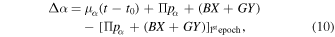
Table 3 lists the astrometric parameters obtained from the MCMC samples. The adopted values and their uncertainties are the medians and standard deviations of the probability density functions, respectively. This approach is possible because all probability density functions are nearly Gaussian. Using the mean instead of the median values would produce differences that are negligible when compared to the uncertainties. The probability density functions for all parameters are shown in Figures 1–3. We describe some basic properties and numerical choices of our MCMC implementation here and provide a general description of the algorithm in Appendix A. Section 4.2 presents statistical tests and discusses the convergence of the Markov chains.
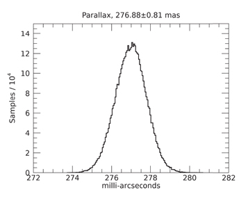
Figure 1. Histogram of posterior samples for trigonometric parallax derived using the combined CTIOPI and CAPS data. Quoted values are the median and standard deviation. The probability density function is based on 5.2 million samples from 52 independent Markov chains.
Download figure:
Standard image High-resolution image
Figure 2. Histograms of posterior samples estimating the probability density functions for parameters derived separately for the CTIOPI and CAPS data sets. Quoted values are the median and standard deviation for each parameter. The discrepancies in proper motion are addressed in Section 3.1. The photocentric semimajor axes are different due to the different filters used for CAPS and CTIOPI, as discussed in Section 3.
Download figure:
Standard image High-resolution image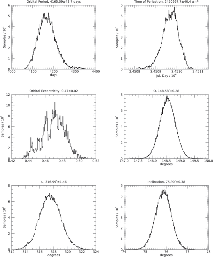
Figure 3. Same as Figure 2 for period, time of periastron passage, eccentricity, and orbit orientation angles derived using the combined CTIOPI and CAPS data.
Download figure:
Standard image High-resolution imageTable 3. Astrometric Resultsa
| Parameter | Value | 1σ Uncertainty | Units |
|---|---|---|---|
| Π | 276.88 | 0.81 | mas |
| d | 3.61 |

|
pc |
| Relative CTIOPI μα | 3973.80 | 0.11 | mas yr−1 |
| Relative CTIOPI μδ | −2508.34 | 0.31 | mas yr−1 |
| Relative CAPS μα | 3966.99 | 0.36 | mas yr−1 |
| Relative CAPS μδ | −2452.87 | 0.40 | mas yr−1 |
| aCTIOPI | 167.76 | 1.83 | mas |
| aCAPS | 201.61 | 1.97 | mas |
| P | 4165.09 | 43.7 | day |
| e | 0.47 | 0.02 | ⋯ |
| T | 2450967.7 ± nP | 40.4 | JD |
| T | 1998.45 ± nP | 0.11 | epoch |
| Ω | 148.58 | 0.28 | degb |
| ω | 316.99 | 1.46 | degb |
| i | 75.90 | 0.38 | deg |
Notes.
aAll quantities refer to the system's photocenter. bMeasured from north to east.Download table as: ASCIITypeset image
All probability density functions are based on the last 100,000 steps of 52 independent 2 million step chains, thus comprising a total of 5.2 million MCMC samples per parameter. No chain thinning was applied. Uniform priors covering parameter intervals much wider than what is physically possible given the observations were used for all parameters (Appendix A.1). The step scale was determined in an adaptive manner according to Equation (15). The process creates a distribution of step sizes centered about a chosen step value for a chosen scaling parameter. We chose the scaling parameter to be trigonometric parallax and the central step value to be 1 mas because that is the typical uncertainty in our astrometric measurement. We then randomly divided or multiplied this central value (1 mas) by a uniformly generated random number between 0 and 10 to create a broad distribution. The other parameters were scaled according to Equation (16) so as to vary in a nearly random fashion on small scales (≲100 steps) while causing the variations of all parameters to have effects of nearly the same magnitude in the large scale of the overall probability density function. This mechanism prevents parameters that heavily influence the overall astrometric motion, such as the very high proper motion, from also dominating the MCMC convergence at the expense of other parameters.
Our joint solution yields a trigonometric parallax of 276.88 ± 0.81 mas, which is in excellent agreement with the Hipparcos parallax for the A component: 276.06 ± 0.28 mas. We therefore detect no depth separation between the A and BC components.
Figure 4 illustrates the orbit solution and observed displacements with the proper motion and parallax solutions subtracted. The shaded contours indicate the 1σ and 3σ uncertainties of the orbit solution based on a Monte Carlo simulation of 10,000 possible orbits given the values and uncertainties in Table 3. The semimajor axis obtained for the CTIOPI IKC-band data (167.76 ± 1.83 mas) was scaled up to match the semimajor axis for the CAPS data (201.61 ± 1.97 mas) for clarity. The smaller semimajor axis in the IKC band reflects the trend toward bluer colors for later T dwarfs in the infrared (Table 1), which decreases the flux difference between the B and C components. The formal solution shows excellent agreement with the data, with 40 out of 52, or 77%, of the observations overlapping the 1σ uncertainty contour, indicating that the formal uncertainties may be slightly overestimated.
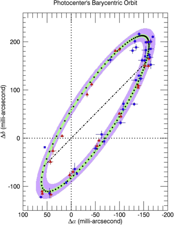
Figure 4. Sky projection of the barycentric orbit of ε Indi BC's photocenter. The filled black circles denote time intervals of approximately 40 days. The shaded contours indicate the 1σ (green) and 3σ (purple) uncertainties on the projected orbit. The observed data (Table 2) are overplotted with the proper motion and parallax subtracted. Blue squares indicate CTIOPI data, and red triangles indicate CAPS data. The CTIOPI data were scaled up to match the semimajor axis of the CAPS data for clarity. The dash-dotted line is the projection of the orbit's major axis.
Download figure:
Standard image High-resolution imageThe integrated light photometric variability of the BC component in the CTIOPI data is 15.9 mmag in the I band. This result is the standard deviation of the BC component's flux, measured by aperture photometry, over all epochs when compared to the sum of the flux of all reference stars, excluding any found to be variable to more than 5 mmag. This value is significantly smaller than the 136 mmag inferred by Koen (2013). Koen noted that his variability data appear to be correlated with seeing and that such a correlation is a clear indication of systemic error. He concluded that the true variability is likely smaller than his formal value. The semimajor axis of the photocenter's orbit is a function of both displacement and flux ratio, and therefore the uncertainty in the semimajor axis can serve as a check on variability. For both data sets, our uncertainties in the semimajor axis are approximately 1% (Table 3), therefore suggesting that the variability must be of that order or smaller. We note, however, that the astrometric observations provide only sporadic time coverage and do not rule out isolated variations in flux as high as the ones noted in Koen (2013). The lower variability is consistent with other studies indicating that, for field-aged T dwarfs, variability is generally on the order of a few percent (e.g., Radigan 2014). Variability data are not available from the CAPSCam data set.
4.1. Dynamical Masses
To obtain dynamical masses from the photocenter's orbit, we followed the method described in van de Kamp (1968) and McCarthy et al. (1991). We summarize the formalism here while providing a detailed example of dynamical mass determination in Appendix B. At any given epoch, define ρ as the magnitude of the photocenter's displacement about the barycenter and p as the projected separation between components B and C. The constant scaling factor from the photocenter's orbit around the barycenter to the relative orbit of component C around B is then p/ρ and can be measured at any epoch for which a resolved image exists. Along with Kepler's third law, this relation yields the system's total mass without regard to the flux ratio of both components in the unresolved observations. To obtain individual masses, define  as the fractional mass of the C component:

Likewise, define  as the fractional flux of the C component in the band used to map the photocenter's displacement.12
The mass ratio is then found by setting
as the fractional flux of the C component in the band used to map the photocenter's displacement.12
The mass ratio is then found by setting

It is therefore necessary to know the flux ratio of the B and C components in one of the bands used to map the photocenter's orbit. The SDSS z band very nearly approximates the CAPSCam overall bandpass (Boss et al. 2009). For this purpose, we used the z-band flux ratio from King et al. (2010; FC/FB = 0.259 ± 0.002). We validated the photometric equivalency assumption by comparing z − J colors obtained with the SDSS z band to colors obtained with CAPSCam for the field of LHS 495, which is very crowded and observed by both surveys. Figure 5 shows the comparison. While there are only a few very red objects, the one-to-one relation is clear in the range including the z − J colors of the B and C components: 2.87 and 3.57, respectively. We therefore adopt ΔCAPS ≈ Δz and add an additional uncertainty of 0.1 mag to the FC/FB flux ratio. We note that any uncertainty depending on the flux ratio will be propagated to the mass ratio of the components but will have no effect on the total mass of the BC system.
Table 4 lists the dynamical masses we obtained from the weighted mean of six epochs of high-resolution imaging, as well as the semimajor axes for the orbits of the B and C components about the BC barycenter. The semimajor axis of the relative orbit of the C component around the B component, the quantity that is used in solving Kepler's third law, is 2.61 ± 0.03 au. The total system mass is 0.138 ± 0.0010 M⊙, or 144.49 ± 1.06 MJup. As previously discussed, this relative semimajor axis and the total system mass are independent of any photometric flux assumption. The adopted best values for the individual dynamical masses are 75.0 ± 0.82 Mjup for the B component and 70.1 ± 0.68 Mjup for the C component. Figure 6 shows the barycentric orbits of the individual components along with the photocenter's orbit and the separations measured in the high-resolution images.
Table 4. VLT/NACO Observations, Semimajor Axes, and Dynamical Masses
| Night | JD | Sep. | σsep. | P.A.a | σP.A. | aBb | σ(aB) | aCb | σ(aC) | MB | σ(MB) | MB | σ(MB) | MC | σ(MC) | MC | σ(MC) |
|---|---|---|---|---|---|---|---|---|---|---|---|---|---|---|---|---|---|
| (mas) | (mas) | (deg) | (deg) | (au) | (au) | (au) | (au) | (M⊙) | (M⊙) | (MJup) | (MJup) | (M⊙) | (M⊙) | (MJup) | (MJup) | ||
| 2004 Nov 11 | 2453323.5 | 894.2 | 2.7 | 140.7 | 0.16 | 1.269 | 0.044 | 1.360 | 0.054 | 0.0722 | 0.0025 | 75.7 | 2.6 | 0.0673 | 0.0018 | 70.5 | 1.9 |
| 2005 Jun 04 | 2453525.5 | 927.7 | 2.3 | 142.5 | 0.10 | 1.266 | 0.043 | 1.350 | 0.048 | 0.0710 | 0.0019 | 74.4 | 2.0 | 0.0666 | 0.0016 | 69.7 | 1.7 |
| 2005 Jul 06 | 2453557.5 | 932.3 | 1.1 | 142.6 | 0.10 | 1.267 | 0.043 | 1.352 | 0.047 | 0.0713 | 0.0019 | 74.8 | 2.0 | 0.0667 | 0.0016 | 69.9 | 1.7 |
| 2005 Aug 06 | 2453588.5 | 934.8 | 2.3 | 142.9 | 0.07 | 1.266 | 0.043 | 1.352 | 0.047 | 0.0713 | 0.0018 | 74.7 | 1.9 | 0.0667 | 0.0015 | 69.9 | 1.6 |
| 2005 Dec 17 | 2453721.5 | 940.4 | 0.6 | 144.1 | 0.10 | 1.268 | 0.043 | 1.357 | 0.046 | 0.0720 | 0.0018 | 75.5 | 1.9 | 0.0672 | 0.0015 | 70.4 | 1.6 |
| 2005 Dec 31 | 2453735.5 | 940.0 | 2.2 | 144.1 | 0.18 | 1.268 | 0.043 | 1.358 | 0.046 | 0.0720 | 0.0018 | 75.5 | 1.9 | 0.0672 | 0.0016 | 70.4 | 1.7 |
| Weighted means | ⋯ | ⋯ | ⋯ | ⋯ | ⋯ | 1.267 | 0.018 | 1.355 | 0.0195 | 0.0716 | 0.0008 | 75.0 | 0.82 | 0.0669 | 0.00064 | 70.1 | 0.68 |
Notes.
aPosition angle of C relative to B measured E of N. Differs by ±180° from photocenter's orbit. bDerived semimajor axis of component's orbit about the BC system's barycenter using the ratio of the photocentric offset to the observed separation at that epoch.Download table as: ASCIITypeset image
4.2. Statistical Tests, Convergence, and Systematic Errors
Figure 7 shows the evolution and convergence of Markov chains for the three astrometric parameters used in dynamical mass determination: trigonometric parallax, semimajor axis, and orbital period. Based on the long burn-in phase of several chains, we conservatively choose to use only the last 100,000 samples. We formally verified the convergence of the 52 Markov chains by applying the Gelman–Rubin statistical test for convergence (Gelman & Rubin 1992).13 Figure 8 shows the results as a function of the length of the chain's burn-in phase. The test measures the extent to which all 52 chains have converged to a stable result, indicated by a value approximating 1.00. The test confirms what is seen graphically in Figure 7—that convergence is obtained after about 1.4 million steps and the chains have completely stabilized in the last 100,000 steps, from which we draw the astrometric parameters.
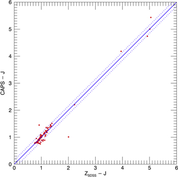
Figure 5. Comparison of the CAPSCam system response function to the SDSS z band for stars in the field of LHS 495. The red dots indicate field objects for which photometry was done on both systems. The solid blue line indicates a one-to-one relation. The dotted lines are the 1σ uncertainties of 0.1 mag about the fit. The z − J colors of the B and C components are 2.87 and 3.57, respectively.
Download figure:
Standard image High-resolution image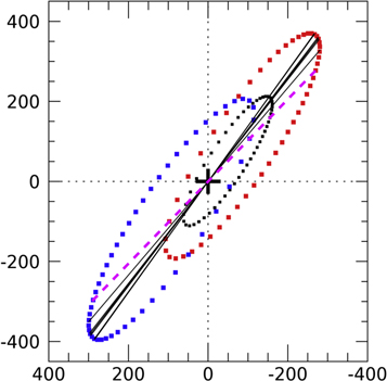
Figure 6. Projected barycentric orbits of ε Indi B (red) and C (blue) plotted along with the photocenter's orbit (black). The solid lines connecting the orbits through the barycenter show the separations at the six epochs of high-resolution imaging. The dashed magenta line is the projection of the semimajor axis. The plotting points represent displacements of approximately 21 days. We refer the reader to Figure 4 for a more detailed description of the photocenter's orbit. The uncertainty contours shown in Figure 4 can be scaled linearly to the orbits of the two components. Figure 13 shows the same orbits without projection effects.
Download figure:
Standard image High-resolution imageFigure 9 shows the correlation plots for all 13 astrometric parameters. Most parameter combinations show low or no correlation with well-defined central values. Combinations of the temporal parameters of proper motions, time of periastron passage, and orbital period show very high correlation, as is to be expected of parameters that determine the photocenter's displacement as a function of the same critical domain. Furthermore, most parameters show mild correlation with the proper-motion parameters, most likely due to the fact that proper motion is by far the dominant source of the system's displacement.
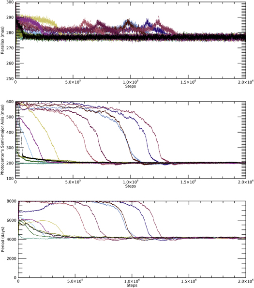
Figure 7. Full 2 million step Markov chains for the three parameters used in mass determination: trigonometric parallax, the semimajor axis of the photocenter's orbit in the CAPS data, and the orbital period. Only 13 out of 52 chains are plotted for clarity. The vertical axes show the full range in which each parameter was allowed to fluctuate, essentially comprising a uniform prior. The chains for trigonometric parallax appear to be wider due to the narrower allowed parameter space, because the trigonometric parallax is heavily constrained by that of ε Indi A. The same chains are plotted using the same colors for all three parameters. Convergence is not evident before 1.4 million steps. We conservatively use only the last 100,000 steps in inferring results.
Download figure:
Standard image High-resolution image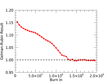
Figure 8. Results of the Gelman–Rubin test for chain convergence. The plot indicates the degree of convergence after the number of steps indicated in the horizontal axis have been removed as the "burn-in" phase. Each dot indicates an increment of 50,000 steps. Results close to 1.00 indicate convergence, which is reached after approximately 1.4 million steps. The results of the test agree well with the chain plots in Figure 8.
Download figure:
Standard image High-resolution image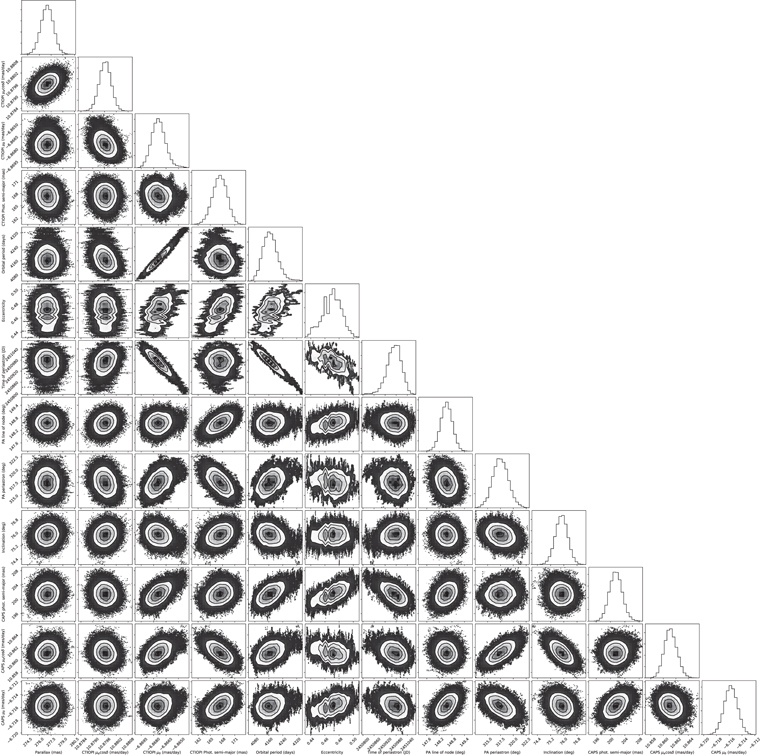
Figure 9. Correlation plots for the 13 astrometric parameters. See the text for discussion.
Download figure:
Standard image High-resolution imageWe save a discuss of the MCMC's acceptance fraction for Appendix A.
4.2.1. Error Analysis of the Mass Derivation
The dynamical masses listed in Table 4 include Gaussian uncertainties propagated via Monte Carlo, which is appropriate for independent random uncertainties. We now examine the possibility of systematic errors in the dynamical masses.
From Appendix B, the quantities necessary for the dynamical mass calculation are the physical semimajor axis of the relative orbit (a), orbital period (P), orbital separation at a given epoch (p), and displacement of the photocenter calculated at the same epoch (ρ). The quantities a and p are functions of the photocentric semimajor axis (α), the trigonometric parallax (Π), and the pixel scale used in the VLT/NACO observations. Given the excellent agreement between the parallax we obtain (276.88 ± 0.81 mas) and the Hipparcos parallax for the A component (276.06 ± 0.28 mas), we can rule out systematic errors in our trigonometric parallax. The pixel scale of the NACO detector was examined in detail by Ginski et al. (2014), who found a mean value of 13.233 ± 0.012 mas pixel–1 based on five globular cluster calibrations between 2008 June 14 and 2012 March 03. This value is within 0.28% of the pixel scale reported by the observatory and used in our calculations, 13.270 mas pixel–1. Propagating this offset leads to a 0.841% increase in the dynamical masses: 0.63 MJup for ε Indi B and 0.59 MJup for the C component. These offsets are within the uncertainties of our reported masses, 75.0 ± 0.82 and 70.1 ± 0.68 MJup, for the B and C components, respectively. The uncertainty in pixel scale caused by any systematics or temporal drift is therefore not a significant source of error and is most likely contributing to the uncertainties we already adopt.
The displacement of the photocenter at the epoch of AO observation ρ and the semimajor axes of the relative physical orbit a are also functions of the photocentric orbit's semimajor axis, α. This last quantity is inferred by the MCMC, which raises the question of whether or not all parameters inferred by the MCMC are correct and not contributing systematic error to the other parameters. The result of the Gelman–Rubin test (Figure 8) strongly suggests that all parameters have converged to their true values. As a further test, we examine parameter correlations and whether or not they could be offsetting each other. For the purposes of mass calculation, the relevant MCMC inferred parameters are α, P, and Π. In principle, these values could contain systematic errors if the sources of motion, trigonometric parallax, proper motion, and orbital motion, are not well separated. Figure 9 shows the correlation plots for all parameters. The parameters α and P show a slight correlation to each other, and α is also correlated to the declination component of proper motion. Correlation is not necessarily a sign of systematic error, but it raises the possibility that those parameters could be contributing to each other in an erroneous manner. To test this, we introduced 4σ systematic errors to the declination component of proper motion, α, and P and held each one of those parameters fixed while testing the MCMC for convergence. In all three cases, the MCMC results did not converge, resulting in multimodal distributions as opposed to the well-defined Gaussian probability density functions shown in Figures 1–3. We therefore conclude that the probability of erroneous interference among the sources of motion in our solution is very low.
5. Discussion
Being the only T dwarfs with known dynamical masses that approach the theoretical hydrogen-burning minimal-mass limit, ε Indi B and C are unique. Konopacky et al. (2010) obtained a total system dynamical mass of 62 MJup for the T5.5+T5.5 binary 2MASS J10210969−304197, from which we infer individual masses of approximately 31 MJup. Dupuy & Liu (2017) reported individual component dynamical masses for six T dwarfs ranging from 31 to 55 MJup. Most recently, Bowler et al. (2018) obtained a dynamical mass of  MJup for the late T dwarf GJ 758 B. These masses are all firmly in the substellar mass range. While the determination of these dynamical masses is a valuable contribution, it is difficult to constrain evolutionary models with masses that are firmly in the substellar domain because of the large degeneracy between mass and age in the brown dwarf cooling track. As an example, Burrows et al. (2001) predicted that a mid-T dwarf could range in mass from about 20 to about 60 MJup if its age was 500 Myr or 10 Gyr, respectively. Both ages are possible within the general galactic disk population. It is therefore not surprising that the components of 2MASS J10210969−304197 and ε Indi C have approximately the same spectral type and vastly different masses, because they probably have very different ages. Because there are no reliable age indicators for isolated older substellar objects, there is little we can learn from them regarding substellar cooling rates. In contrast, objects with masses close to the stellar–substellar limit allow us to test a boundary value of the theory of substellar structure and evolution.
There is broad consensus that T dwarfs are substellar objects (e.g., Burrows et al. 2001; Kirkpatrick 2005). Table 5 lists the most widely used evolutionary models for substellar objects and the temperatures at which they predict the stellar–substellar boundary. King et al. (2010) inferred effective temperatures in the range of 1300–1340 and 880–940 K for ε Indi B and C, respectively. These temperatures are in good agreement to those inferred by Filippazzo et al. (2015) for field-aged objects of spectral types T1 and T6: 1200 and 900 K. We see, therefore, that virtually the entirety of our theoretical understanding of T dwarfs would be significantly erroneous if ε Indi B and C were stellar objects. As we are about to discuss, problems with the theory do exist. However, a scenario that makes ε Indi B and C, or even only the B component, a star is extremely unlikely; all models listed in Table 5 would have to be overpredicting the temperature of the stellar–substellar boundary by several hundred K. And yet the masses we obtained are remarkably high, given our current understanding of substellar structure and evolution. There is strong evidence from photometry, spectroscopy, and adaptive optics imaging that the B and C components have different luminosities and therefore must have different masses given their common age (Sections 1 and 4.1). However, even if we disregard flux ratio, dividing the total system mass by 2 means that the most massive component cannot have a mass under 72.5 MJup. We note also that, while the ε Indi system has slightly subsolar metallicity (Table 1), stars with [Fe/H] ≈ −0.1 are common in the solar neighborhood and should be included when considering the (sub)stellar population as a whole (e.g., Hinkel et al. 2014).
Table 5. Summary of Predictions for the Stellar–substellar Boundarya
| Study | Type | H-burning | H-burning | H-burning | Metallicityb | Min. Stellar | Atmospheric |
|---|---|---|---|---|---|---|---|
| of Study | Mass (MJup) | Teff (K) | log(L/L⊙) | (Z/Z⊙) | Radius (R/RJup) | Properties | |
| Burrows et al. (1993, 1997) | Model | 80.4 | 1747 | −4.21 | 1.28 | 0.84 | Gray with grains |
| Burrows et al. (1993) | Model | 98.5 | 3630 | −2.90 | 0.00 | 0.89 | Metal-freec |
| Baraffe et al. (1998) | Model | 75.4 | 1700 | −4.26 | 1.28 | 0.84 | Nongray without grains |
| Chabrier et al. (2000) | Model | 73.3 | 1550 | −4.42 | 1.28 | 0.86 | "DUSTY" grains do not settle |
| Burrows et al. (2001) | Model | 73.3–96.4 | ⋯ | ⋯ | Various | ⋯ | Discussion of various models |
| Baraffe et al. (2003) | Model | 75.4 | 1560 | −4.47 | 1.28 | 0.81 | "COND" clear and metal-depletedd |
| Saumon & Marley (2008) | Model | 78.6 | 1910 | −4.00 | 0.87 | 0.89 | Cloudless |
| Saumon & Marley (2008) | Model | 73.3 | 1550 | −4.36 | 0.87 | 0.91 | Cloudy, fsed = 2 |
| Baraffe et al. (2015) | Model | 73.3 | 1626 | −4.30 | 1.00 | 0.89 | "BT-Settl" cloud model |
| Dieterich et al. (2014) | HR survey | ⋯ | 2075 | −3.90 | Field | 0.86 | ⋯ |
| Dupuy & Liu (2017) | Mass survey | 70 | ⋯ | ⋯ | Field | ⋯ | ⋯ |
| ε Indi B | Mass | 75.0 ± 0.82 | 1320e | −4.70e | 0.74 | 0.83 | ⋯ |
| ε Indi C | Mass | 70.1 ± 0.68 | 910e | −5.23e | 0.74 | 0.85 | ⋯ |
Notes.
aAdapted and updated from Table 8 of Dieterich et al. (2014). bWe adopt the solar metallicities of Caffau et al. (2011) as the "true" solar value. With the exception of the zero-metallicity case of Burrows et al. (1993), all models were meant as solar metallicity when they were published. Here we scaled their metallicities to reflect the new values of Caffau et al. (2011). See Allard et al. (2013) for a discussion of recent revisions to solar abundances. cAn artificial case meant to illustrate the significance of metallicity in determining the parameters of the stellar–substellar boundary. dIn this case, metals are sequestered in grains that settle below the photosphere. eKing et al. (2010).Download table as: ASCIITypeset image
Figure 10 shows two color–magnitude diagrams based on the data from the Database of Ultracool Parallaxes maintained by Trent Dupuy14 (Dupuy & Liu 2012; Dupuy & Kraus 2013). While the C component appears to be slightly blue, neither component stands out from the general field population. Any correct theoretical framework must allow such massive objects to be substellar and also provide an appropriately fast cooling rate so that they reach the T spectral type in a time that must be smaller than the upper bound on the system's age, the age of the Galaxy.
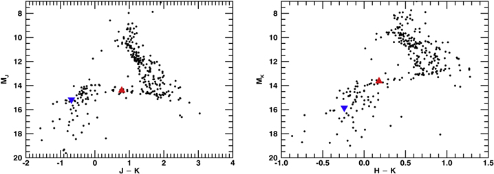
Figure 10. Color–magnitude plots showing ε Indi B plotted as a red triangle and C as a blue inverted triangle. While the C component appears to lie slightly blueward of the center of the sequence, neither component can be distinguished from the general population. While some objects are clearly deviant from the sequence, in the interest of completeness, we did not exclude any data from T. Dupuy's database.
Download figure:
Standard image High-resolution imageTable 5 lists several studies regarding the properties of the stellar–substellar boundary from both theoretical and observational perspectives. All theoretical treatments agree that as a general trend, higher opacity moves the end of the stellar main sequence downward in mass, luminosity, and effective temperature. The overall opacity driving the trend is a complex function of metallicity and atmospheric parameters, such as the presence of silicate grains and their sedimentation rate. The result is a wide range of predictions for the fundamental parameters of the smallest and least-massive possible stellar objects. At present, the models that address the effects of different metallicities and atmospheric conditions tend to consider extreme values, so it is difficult to ascertain what the models would predict in the case of ε Indi's slightly subsolar metallicity. We can gain some insight from the fact that the models listed in Table 5 have adopted different values for the zero-point solar abundances, and the offsets among those different values provide a limited range of metallicities for comparison.
Given the uncertainties on the dynamical mass of ε Indi B (75.0 ± 0.82 MJup), none of the models listed in Table 5 can be strictly ruled out as far as predicting its substellar nature. However, Chabrier et al. (2000); the cloudy version of Saumon & Marley (2008); and Baraffe et al. (2015), the only evolutionary model in that family to use updated metallicities (Caffau et al. 2011) and an adaptive cloud model (Allard et al. 2013), do so only marginally and predict masses ∼2σ away from our best values.
Our results are not compatible with the possibility of the stellar–substellar mass boundary being at 70 MJup, as claimed by Dupuy & Liu (2017). We note, however, that their own data (Dupuy & Liu 2017, Table 11 and Figure 3) are amenable to broad interpretation and that the mean of the uncertainty of their dynamical masses that fall within the 70 MJup range is 5.6 MJup. Finally, Dieterich et al. (2014) examined luminosity, temperature, and radius trends in the early L dwarf range and did not address the question of the minimum stellar mass directly. The claims in Dieterich et al. (2014) therefore cannot be directly tested by the dynamical masses we report here.
Assuming that a given model predicts that such massive objects would be substellar, another relevant question is whether or not the model can provide a fast enough cooling rate to make ε Indi B and C reach T dwarf temperatures. Filippazzo et al. (2015) established luminosities (log(L/L⊙)) of −4.6 and −5.0 for T1.5 and T6 dwarfs, respectively, and effective temperatures of 1200 and 900 K for field-aged objects. Most models we consider in Table 5 cannot make such massive objects reach those temperatures in times shorter than the age of the Galaxy. Even at an age of 10 Gyr, the Burrows solar-metallicity models (Burrows et al. 1997, 2001) predict the effective temperature of a 75 MJup object to be 200–400 K hotter than 1200 K, thus placing ε Indi B in the mid-to-late L spectral type range. The discrepancy for the C component is slightly smaller, on the order of 150 K. The same models can accommodate the luminosities and temperatures of both components at 10 Gyr if the opacity is decreased by setting [Fe/H] = −1.0; however, that is a factor of 7.4 less than the observed metallicity of ε Indi A ([Fe/H] = −0.13; see Table 1). See Figures 1, 4, 5, and 8 of Burrows et al. (2001) for graphical representations of these models.
The cloudy version of Saumon & Marley (2008) and the "DUSTY" models of Chabrier et al. (2000) are similar to each other at ages greater than 4 Gyr. They predict temperatures about 400 K above the temperatures from the Filippazzo et al. (2015) field sequence. See Figure 3 of Saumon & Marley (2008) for graphical representations of these models.
The "COND" models of Baraffe et al. (2003) and the cloudless version of Saumon & Marley (2008) deliberately simulate less opaque atmospheres to investigate the possibility that atmospheric silicate grains either do not form or settle quickly below the photosphere. These models predict considerably faster cooling rates and can reach the temperatures of ε Indi B and C at ages ≲10 Gyr if their masses are slightly beyond the lower bounds in the 1σ uncertainties we obtained. The ε Indi system would then have to be very old to fit these isochrones. See Figure 2 of Saumon & Marley (2008) for graphical representations of these models. The K5V A component has been associated with the small moving group of the same name (Eggen 1958), and age estimates for that moving group range from 5 to 6.2 Gyr (Cannon & Lloyd 1970; Soubiran & Girard 2005; King et al. 2010). However, the proposed moving group is small, with only 15 stars identified by Eggen (1958), and Kovacs & Foy (1978) cast doubt on its membership and existence. Lachaume et al. (1999) noted that while the chromospheric activity of ε Indi A indicates an age of 1–2.7 Gyr, the system's Galactic kinematics are consistent with a much older age of ≳7.4 Gyr. It is therefore plausible that the system is old, but, as is evident from this discussion, the ages of low-mass main-sequence stars are notoriously difficult to determine. A greater problem may be that while cool brown dwarfs that have passed the L–T transition are thought to have clear atmospheres, the spectra of L dwarfs are well replicated by models that include some amount of silicate grains (e.g., Allard et al. 2013). The conditions assumed in these clear models may therefore not be a realistic representation of a T dwarf's cooling history. Nevertheless, we note that the "COND" models of Baraffe et al. (2003) and the cloudless models of Saumon & Marley (2008) come considerably closer to matching the parameters of ε Indi B and C than the more opaque models also listed in Table 5. From an intuitive perspective, it may seem surprising that a mass difference of only 5 MJup causes such a large difference in spectral type and effective temperature. In the preceding analysis, we discussed the plausibility of several evolutionary scenarios regarding ε Indi BC as a coeval system and not as individual components. We have therefore implicitly tested whether the models can explain their differentiation. As a general trend, it seems more difficult to explain the hotter temperatures of both components rather than their difference. We note that the evolution of substellar objects lying very close to the hydrogen-burning limit is poorly understood, in large part because model grids lack a finer resolution in that critical point. It is possible that objects very close to the hydrogen-burning limit may have markedly slower evolution. If ε Indi B falls into this scenario, then our attempts to interpolate its evolution from the available coarser evolutionary grids may be misguided.
6. Conclusions
We inferred the dynamical masses of ε Indi B and C using unresolved photocentric astrometric data, resolved adaptive optics images, and MCMC techniques. The dynamical masses we obtained, 75.0 ± 0.82 and 70.1 ± 0.68 MJup for the B and C components, respectively, are surprisingly high and challenge our understanding of the stellar–substellar mass boundary.
Our analysis highlights the strengths and weaknesses of different approaches to understanding the structure and evolution of two old and massive brown dwarfs. It is clear that the current models underpredict the upper mass limit and/or the necessary cooling rates for ε Indi B and C, with less opaque models coming closer to replicating the observed parameters. The system's slight negative departure from solar metallicity is of the same order as the differences among the solar abundances chosen by different models listed in Table 5. The lack of a clear trend linking metallicities to fundamental parameters in Table 5, as well as the lack of a clear displacement from the field sequence in color–magnitude diagrams (Figure 10), suggest that small changes in metallicity are likely not a dominant factor in determining the structure and evolution of brown dwarfs. This result supports the theoretical argument to the same effect first proposed by Burrows et al. (2001).
Dieterich et al. (2014) examined the fundamental parameters of the nearby field L dwarf population and found that the models likely underpredict the luminosity and effective temperature of objects at the stellar–substellar boundary. While that study did not directly address mass, the most fundamental of all (sub)stellar parameters, it noted that if the higher-than-expected temperatures and luminosities were due to models overestimating opacities, then a higher limit for substellar masses should also be expected. The high dynamical masses of ε Indi B and C support that explanation.
Finally, we note that we now have two well-characterized brown dwarfs with precise dynamical masses very close to the stellar–substellar boundary, spatially resolved spectra and photometry, and well-constrained metallicities from their main-sequence primary component. The thorough modeling of the ε Indi system using precise empirical input values would provide considerable insight into outstanding theoretical issues regarding the stellar–substellar boundary.
We thank John Gizis and G. Fritz Benedict for helpful discussions and the anonymous referees, whose insights have helped to greatly improve the article. SBD acknowledges support from the National Science Foundation Astronomy and Astrophysics Postdoctoral Fellowship Program through grant AST-1400680. We thank the David W. Thompson Family Fund for support of the CAPSCam astrometric planet search program and the Carnegie Observatories for continued access to the du Pont telescope. The development of the CAPSCam camera was supported in part by NSF grant AST-0352912. The CTIOPI program is made possible through the SMARTS Consortium and NSF grants AST-0507711, AST-0908402, AST-1412026, and AST-1715551. This research has made use of the SIMBAD database, operated at CDS, Strasbourg, France. This research has made use of the services of the ESO Science Archive Facility. This research has made use of IRAF, which is distributed by the National Optical Astronomy Observatory, operated by the Association of Universities for Research in Astronomy (AURA) under a cooperative agreement with the National Science Foundation.
We wish to honor the memory of our colleague Sandra Kaiser, an integral member of the CAPS team who died while this work was being done. Carnegie is not the same without Sandy.
Appendix A: The MCMC Algorithm and Its Implementation
The goal of the MCMC is to generate samplings from posterior probability density functions that can then be interpreted through Bayesian inference as the probability density functions for parameters of interest. We found that solving the astrometric problem described in Section 3 poses two specific challenges. First, step sizes must be generated in an adaptive manner that prevents a single parameter from dominating the overall evolution of the probability density function. This is particularly problematic because the orbit's orientation angles may take on values that minimize or maximize the effect of a given direction of motion while probing the parameter space. Second, a mechanism must exist to cause any chains stuck in local probability maxima to continue to evolve. We developed a modification of the Metropolis–Hastings MCMC procedure that specifically addresses these issues in the context of the astrometric problem. Here we describe the general case assuming a single astrometric data set. The extension to two or more data sets is not difficult and is discussed in Section 3. The IDL suite of codes and detailed documentation are available for download at github.com/SergeDieterich/MCMC_SD and archived in Zenodo (Dieterich 2018).
This standard implementation also allows the user to set any parameter to a fixed number so as to solve a specific subset of the astrometric problem, such as a resolved visual binary or the trigonometric parallax for a single star. Readers are encouraged to contact SBD to discuss nonstandard uses.
Assuming Gaussian uncertainties in the observed positions of the photocenter (Table 2), the probability that a given set of astrometric parameters matches the data is expressed as

where  refer to Equations (10) and (11). Equation (14) is valid for independent parameters. This is the case for displacements and uncertainties in declination and right ascension because both telescopes used here are polar-mounted, meaning their jitter has separate sources for the two orthogonal axes. The uncertainties due to atmospheric seeing are also known to be isotropic. The logarithm facilitates numerical computations for very small probabilities while still preserving an easy way to compare probability ratios. The term K in Equation (14) expresses the probability introduced by the choice of prior. However, because we use constant uniform priors (Appendix A.1), K is a constant and cancels out when we take the ratio of probabilities between two MCMC steps to evaluate whether the chain will advance.
The rule for deciding if a given step advances the Markov chain is a standard Metropolis–Hastings procedure. After a step changes the values of all astrometric parameters simultaneously, the Markov chain will remain in the new location if the ratio of the new to the previous solution probability is greater than a uniformly distributed random number in the range of zero to one and will return to the previous location otherwise.
The step generator for each parameter is of the form

where A and C are randomly discrete ±1; B is a random number between zero and the user-specified "step multiplier" parameter, which governs the scale of the step distribution; and D is a fixed step size for a chosen "scaling parameter." The partial derivative ensures that in the long run of hundreds or more steps, all parameters will contribute more or less equally to the evolution of the Markov chain toward a solution. The partial derivative is an order-of-magnitude calculation and approximated by measuring the slope of the overall displacement in the astrometric solution, taking the last two steps into account:

In the work discussed here, we chose trigonometric parallax as the scaling parameter and set D = 1 and the step multiplier equal to 10 so that for each parameter in each step, 0.1 ≤ BC ≤ 10. That setup caused all parameters to change the value of the overall solution in a scale similar to changing the trigonometric parallax by 1 mas for each step in the long run, but with ABC causing considerable variation in the small scale of ≲100 steps. We set C = −1 at every five steps for all parameters so as to provide small adjustments in parameter space that would otherwise be difficult to achieve due to the simultaneous and independent nature of the parameter steps.
A.1. Avoiding Local Maxima and Enabling Broad Uniform Priors—The "Spider" Mechanism
Little is known a priori about the specific configuration of an unresolved binary system other than very broad constraints that can be inferred from the design of the observations and the nature of the data. As examples, a binary system's unresolved nature means that its projected semimajor axis must be below the telescope's resolution, and the fact that we see nonlinear displacements at periods greater than 1 yr means that the temporal baseline of the observations is comparable to the orbital period. We use only these broad assumptions in defining the ranges of parameter space to be explored, thus effectively establishing broad uniform priors. Given the wide diversity in binary systems and the convoluted nature of the parameter space we are exploring, we believe there is little justification to assume any other form of prior. It is therefore important that our MCMC algorithm explore the entirety of this broad parameter space and lose the dependence on the discrete initial values of each chain.
One of the difficulties we encountered in using MCMC algorithms was the prevalence of local maxima in probability space that did not correspond to the true solution. This problem persisted even after employing the adaptive step scaling. To solve this problem, we devised an additional step-scale rule that causes a chain to take very large jumps in parameter space, probe the new region, and then compare the relative probabilities of the old and new regions to decide in which region the chain should continue to evolve. This method is similar to the "Snooker" updater of ter Braak & Vrugt (2008). This mechanism gives the chains the ability to jump between local probability maxima until they land in the region of the absolute probability maximum. We call this condition the "spider" mechanism, in analogy to a spider that extends one of its legs to a distant region, probes that locality, and then decides whether or not to move its entire body there or to retract its leg.
At every 200 steps, one astrometric parameter is randomly selected and jumps to a new random location within its allowed range. The Markov chain then evolves normally for 100 steps. If the mean solution probability of the 100 steps after the jump is less than the mean probability of the 100 steps before the jump, the chain will return to its pre-jump location or continue in the new vicinity. This mechanism is most effective in causing large jumps early on during the MCMC evolution, when all probabilities are likely to be very low. Once the chains resemble the final probability density functions, most spider jumps are rejected or cause shifts that are comparable to the normal step process. This ensures that the ergodicity of our MCMC algorithm is not broken by this additional mechanism (Andrieu & Moulines 2006). Figure 11 shows the probability density functions for trigonometric parallax produced with and without the spider mechanism. Whereas the location of the histogram's peak changes very little as a result of the spider mechanism, several chains that were stuck in a local maximum around 290 mas move to the main peak as a result of employing the spider mechanism.
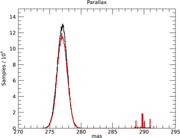
Figure 11. Comparison of the probability density function histograms for trigonometric parallax produced while employing the spider mechanism (black) and without the spider mechanism (red). While the locations of the Gaussian peaks are very nearly the same, the probability density function produced without the spider mechanism shows a spurious local maximum around 190 mas. This case is typical of all parameters.
Download figure:
Standard image High-resolution imagePerhaps most importantly, the spider mechanism eliminated the need for educated guesses as to a starting value for each chain, thus minimizing the effect of unintentional priors. With the exception of trigonometric parallax, which was strongly constrained by that of the ε Indi A component, the starting values for all other parameters covered a broader range than those reasonably deduced from the setup of the observations.
At large step numbers, as long as the algorithm converges, the step size described in Equation (15) stabilizes and becomes independent of the current state of the chains, ensuring that our MCMC algorithm remains ergodic (Andrieu & Moulines 2006). We demonstrated in Section 4.2 that our algorithm converges, ensuring that the step becomes independent of the chain state after the burn-in phase.
A.2. Computational Performance
The probability density functions shown in Figures 1–3 show the last 100,000 steps of 52 chains of 2 million steps each. Because each chain is completely independent from the other chains, the IDL code can be run in parallel by running it in multiple IDL sessions with identical starting parameters. A procedure included in the code distribution can be used to easily consolidate the results from multiple sessions. Running four simultaneous sessions with 13 chains each and 2 million steps per chain took about 10 hr in a MacBook Pro with an Intel i7 dual core processor.
The acceptance fraction as a function of chain evolution is shown in Figure 12. The overall acceptance fraction upon convergence is low, at only about 3.5%. This low fraction may be due to the choice of step scaling or simply a result of the complex nature of the multiparameter space being probed. The trends in Figure 12 follow the same pattern as those in Figure 8.
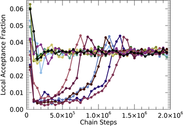
Figure 12. Acceptance fraction for 13 chains, shown as the fraction at every 50,000 interval. The overall low rate may be due to the nature of the parameter space and its high dimensionality or the choice of step scaling.
Download figure:
Standard image High-resolution imageAppendix B: Solving for Individual Masses—An Example
We now discuss the problem of solving for dynamical masses given the photocenter's orbit in detail and carry through a pedagogical example. Figure 13 illustrates the several orbits involved in the problem as seen from above the orbital plane, with no projection effects, and with the orbital major axes aligned with the vertical axis. These orbits are as follows.
- 1.The orbit of the photocenter about the barycenter, traced by black dots. This orbit is the one mapped by the astrometric observations and is the starting point for the derivation of masses. Here we have a choice of using the photocentric orbit traced by the CTIOPI observations or the slightly larger orbit traced by the CAPS observations. We choose the orbit traced by the CAPS observations for reasons that will become clear shortly.
- 2.The orbit of ε Indi B, the more massive component, about the barycenter, traced by large blue squares.
- 3.The orbit of ε Indi C, the less massive component, about the barycenter, traced by small red squares.
- 4.The relative orbit of the C component around the B component is not explicitly shown. However, this orbit can be traced by assuming the position of component B to be static and drawing separation vectors toward component C through the barycenter. This relative orbit is the orbit used in solving Kepler's third law to obtain the sum of the components' masses.
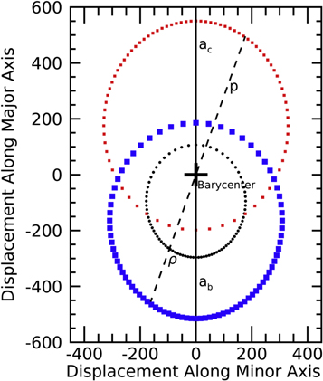
Figure 13. Several orbits involved in the dynamical mass problem, shown without projection effects. The large blue squares represent the orbit of the more massive components (B) about the barycenter. The small red squares show the orbit of the C component about the barycenter. The black dots trace the observed orbit of the photocenter about the barycenter. The dashed line indicates the separation between the B and C components measured on 2005 August 6 (Table 4).
Download figure:
Standard image High-resolution imageThe solution to the problem lies in the fact that all four orbits have the same eccentricity and their orientation in space may change only by 180°, depending on which point is placed at a focus. It is our task, then, to scale the size of these orbits based on the available photocentric orbit solution, the resolved epochs of astrometry, and the system's flux ratio so as to obtain the mass sum and mass ratio for the BC system.
The dashed line connecting the orbit of the B component (blue) to the orbit of the C component (red) represents the separation between the components measured with adaptive optics on 2005 August 6 (Table 4). We define this separation as p and define ρ as the photocenter's displacement in its orbit about the barycenter at the same epoch. The quantity ρ can be calculated from Equations (1) and (2), setting the proper motion μ and parallax Π to zero. The fraction p/ρ is then the constant scaling factor between the observed orbit of the photocenter and the relative orbit of component C about component B. One clearly resolved measurement of the separation p is all that is necessary to establish this relation. Out of the six separation measurements in Table 4, we pick the one from this epoch as an example because it yields the results that are closest to the final weighted averages. From Table 4 and calculating the photocentric displacement from the model yields p/ρ = 934.8 mas/260.1 mas = 3.594. From this scaling relation, we can establish the semimajor axis of the relative orbit based on the observed orbit of the photocenter and its semimajor axis α (Table 3),

which, divided by the trigonometric parallax, yields a = 072458/027688 = 2.617 au. We then use Kepler's third law of planetary motion expressed in solar system units,

to find the system's total mass:  .
.
Two points are worth noting here from an observational perspective. First, we note that starting from an orbit done entirely on small telescopes and with seeing-limited conditions, we were able to obtain the mass sum with a single high-resolution observation. The ability to do so greatly facilitates the overall observational plan, because time in high-resolution facilities is usually more scarce than time in seeing-limited small telescopes. Second, we note that we obtained the mass sum with no explicit knowledge of the flux ratio between the components. That dependence is canceled out in the α/ρ factor in Equation (17). We could just as easily have used the smaller CTIOPI semimajor axis and obtained the same result. This point is significant because obtaining the correct flux ratio in a close binary is often challenging, and it is sometimes easier to infer individual masses in indirect ways based on the mass sum, such as when the primary mass may be known from a mass–luminosity relation.
Now that the total system mass has been established, we turn our attention to obtaining the mass ratio between the B and C components, and therefore individual masses. Recalling Equation (12), we define the fractional mass of the secondary (C) component as

and the fractional flux of the secondary component in an equivalent manner as

Because the flux ratio between the two components affects the overall photocentric displacements that trace the photocenter's orbit, it is crucial that the fluxes in Equation (19) be measured in the same band that was used for the astrometric observations or that a reliable color transformation be used. In most cases, the high-resolution and astrometric observations are done in different filters, and color transformations become relevant. Here we use the semimajor axis from the CAPS orbit because, in Section 4.1 and Figure 5, we demonstrated that the effective band of CAPSCam is equivalent to the z band, for which the VLT/NACO flux ratio is known (Table 1).
We then come to the equation first introduced as Equation (13),

This equation states that the fractional mass and fractional flux of the secondary component play opposite roles in displacing the photocenter from the position of the barycenter. To motivate Equation (21), we refer back to Figure 13. Consider first the hypothetical case where the secondary component contributes no light. That is usually the assumption when searching for astrometric perturbations due to exoplanets. In that case, all light comes from the primary component, and the photocentric orbit (black) and the orbit of the primary component (blue) become the same. The semimajor axis of the photocenter's orbit α is then equal to aB,  is equal to zero, and we recover the usual relation for the location of the components of a binary system about the barycenter: M1a1 = M2a2. At the other extreme, consider the case of an equal-mass and equal-luminosity binary where
  . The symmetry of the configuration then dictates that the photocenter is placed exactly at the barycenter, Equation (21) diverges, and no photocentric displacement exists. Another interesting case happens when the asymmetry in mass and luminosity between the two components is small. A small photocentric displacement may then be detected, and the photocenter's orbit then mimics the other extreme: a very faint brown dwarf or exoplanet orbiting a much more massive and luminous star. Detecting the location of the secondary component in the high-resolution observation or establishing an upper limit for its flux is critical for breaking this degeneracy and distinguishing between two very different astrophysical configurations.
From Table 1, and transforming magnitudes into fluxes,  = 0.206. Using the mass sum determined from Kepler's third law (Equation (18)) and the ratio p/ρ, it is then trivial to solve Equation (21) for individual masses, yielding
  and MC = 0.0668 M⊙. These values are very close to the final values in Table 4, obtained using more data and Monte Carlo error analysis: MB = 0.0716 ± 0.0008 and MC = 0.0669 ± 0.00064 M⊙.
Footnotes
- 10
Small and Moderate Aperture Research Telescopes; www.astro.gsu.edu/~thenry/SMARTS.
- 11
- 12
The quantities that we denote as
 and have traditionally been called B and β, respectively. We use a different notation to avoid confusion with the system's B component.
 - 13
Implemented in IDL by Simon Vaughan, University of Leicester, https://www.star.le.ac.uk/~sav2/idl/rhat.pro.
- 14
Currently hosted at http://www.as.utexas.edu/~tdupuy/plx/Database_of_Ultracool_Parallaxes.html.

