


ABSTRACT
We use the detailed 3D whole-prominence fine structure model to produce the first simulated high-resolution ALMA observations of a modeled quiescent solar prominence. The maps of synthetic brightness temperature and optical thickness shown in the present paper are produced using a visualization method for synthesis of the submillimeter/millimeter radio continua. We have obtained the simulated observations of both the prominence at the limb and the filament on the disk at wavelengths covering a broad range that encompasses the full potential of ALMA. We demonstrate here extent to which the small-scale and large-scale prominence and filament structures will be visible in the ALMA observations spanning both the optically thin and thick regimes. We analyze the relationship between the brightness and kinetic temperature of the prominence plasma. We also illustrate the opportunities ALMA will provide for studying the thermal structure of the prominence plasma from the cores of the cool prominence fine structure to the prominence–corona transition region. In addition, we show that detailed 3D modeling of entire prominences with their numerous fine structures will be important for the correct interpretation of future ALMA observations of prominences.
Export citation and abstract BibTeX RIS
1. INTRODUCTION
Solar prominences are regions of dense and cool plasma embedded in much hotter and significantly less dense corona. Prominences owe their existence to the coronal magnetic field. It supports the dense prominence material against solar gravity and insulates it from the hot coronal environment. Quiescent prominences exhibit rather stable large-scale structures with lifetimes ranging from several days to a few months. However, their small-scale structures—with dimensions of less than 1000 km—are highly dynamic on timescales of a few minutes. On the other hand, active solar prominences have very dynamic large-scale structures and typical lifetimes of a few hours or less.
It is generally understood that the plasma of the quiescent prominences is located in dips of the magnetic field. However, the detailed properties of the prominence plasma and its spatial distribution along the prominence fine structures still remain an open question. For reviews of solar prominences we refer the reader to the works of Tandberg-Hanssen (1995), Labrosse et al. (2010), Mackay et al. (2010), proceedings of the IAU 300 Symposium on the Nature of Prominences and their role in Space Weather (Schmieder et al. 2014), or the recent book Solar Prominences (Vial & Engvold 2015).
Radio observations at submillimeter/millimeter (SMM) wavelength provide a useful tool for diagnostics of the thermal properties of the solar plasma. This is because the source function is the Planck function, which is proportional to the kinetic temperature, and the specific intensity is proportional to the brightness temperature (the Rayleigh–Jeans law). Thus the observed specific intensity at the SMM wavelengths can be used to derive the kinetic temperature of the solar plasma—see, e.g., Loukitcheva et al. (2004) and Heinzel & Avrett (2012). However, such derivation of the kinetic temperature is not entirely straightforward. It can only be performed in cases where at least two simultaneous observations are obtained at SMM wavelengths, and where the prominence observed at one is optically thin and that at the other is optically thick. The kinetic temperature can also be derived from a single observation at SMM wavelength if simultaneous observations in a different spectral range—e.g., the Hα line in the optical domain—are available (see Heinzel et al. 2015a).
For prominences such a temperature diagnostics has until now been performed mostly using a single-dish aperture. The first SMM observations of an active prominence were performed by Harrison et al. (1993). Bastian et al. (1993) later studied several prominences and filaments using observations at two different SMM wavelengths. A further study was performed by Irimajiri et al. (1995) using observations at three different SMM wavelengths. However, such observations from single-dish apertures provide only limited spatial resolution and thus cannot be used to determine the thermal properties of the prominence fine structures.
This will change with the advent of observations of the Sun by the Atacama Large Millimeter/submillimeter Array (ALMA)—the first cycle of solar observations will take place between 2016 December and 2017 April. ALMA will perform solar observations in special observing modes (Karlický et al. 2011) with an unprecedented spatial resolution, thus providing new insights into the temperature structure of small-scale features of the solar atmosphere. The potential contribution of ALMA to solar science was summarized by Wedemeyer et al. (2016).
ALMA represents a new type of observatory for studying solar prominences. It is thus important to understand the extent to which the prominences at the limb and on the disk (filaments) will be visible in ALMA observations and how well their fine structures will be resolved. To correctly interpret the upcoming ALMA observations of prominences we also need to understand how the thermal structure of the prominence plasma will appear in various SMM wavelengths. The question of visibility of the prominence fine structures in the ALMA observations was recently addressed by Heinzel et al. (2015a). These authors used Hα coronagraphic observations of a quiescent prominence to derive the visibility of the prominence fine structures at various ALMA wavelengths. However, this approach can visualize only the cooler structures that are detected in Hα. The spatial resolution that can be achieved by such a technique depends on the original resolution of the Hα observations used. In Heinzel et al. (2015a), the spatial resolution of the synthetic ALMA images was of the order of 1 arcsec. While this does not reach the best potential resolution of ALMA (see, e.g., the discussion in Wedemeyer et al. 2016), it is similar to the resolution that will be achieved in the upcoming ALMA solar observations (Cycle 4). The difference between the present and potential ALMA resolution is due to the fact that the ALMA observatory is still at the development stage and its capabilities will improve over the coming years.
The aim of the present paper is to show the extent to which both the large-scale and small-scale structures of prominences at the limb and filaments on the disk might be visible in the ALMA observations. For this purpose we construct the first synthetic high-resolution images of simulated prominences obtained at SMM wavelengths, covering a broad range that encompasses the full potential of ALMA. The high spatial resolution of these simulated observations is achieved by use of the state-of-the-art high-resolution 3D Whole-Prominence Fine Structure (WPFS) model of Gunár & Mackay (2015a). This model is then combined with a visualization method adapted from Heinzel et al. (2015a). The visualization method can be applied to any model with prominence-like conditions to produce synthetic images at the wavelengths covered by ALMA.
The 3D WPFS model employed here represents an entire prominence with its small-scale structures. It provides a detailed description of the temperature and pressure structure of the prominence plasma when it is distributed along numerous fine structures. These prominence fine structures are located in the dips of the magnetic field structure created by the 3D nonlinear force-free (NLFF) field simulations of Mackay & van Ballegooijen (2009). More details about the method used to produce prominence fine structures located in the NLFF dips can be found in Gunár et al. (2013b). Reviews of the simulations of the prominence magnetic field structure can be found in Mackay et al. (2010), van Ballegooijen & Su (2014), or Gunár (2014).
In the present paper we use the same configuration of the 3D WPFS model as was used by Gunár & Mackay (2015a). The evolution of this modeled prominence was studied by Gunár & Mackay (2015b) and the basic physical properties of its plasma and magnetic field distributions by Gunár & Mackay (2016).
The present paper is structured as follows. We present the basic method for synthesis of the SMM radio continua in Section 2. In Section 3 we describe the application of the synthesis of SMM radio continua to the 3D WPFS model, and in Section 4 we present the synthetic maps of the brightness temperature and optical thickness of the modeled prominences. In Section 5 we discuss our results and in Section 6 we offer our conclusions and analyze the benefits and challenges that the ALMA observations of prominences will bring.
2. SYNTHESIS OF SMM RADIO CONTINUA
In the SMM radio domain the specific intensity Iν emergent from the prominence at the limb is given as (e.g., Heinzel et al. 2015a)

where Bν(T) is the Planck source function, the infinitesimal change in the optical depth dtν is given as

and τν is the total optical depth along a geometrical path of length L. The parameter κν represents the absorption coefficient. We can then rewrite Equation (1) in the form

which can be easily solved numerically.
For a filament on the solar disk the emergent specific intensity Iν is given as

where  is the background disk intensity.
The opacity in the SMM radio domain under characteristic prominence conditions is dominated by the hydrogen free–free continuum (Rybicki & Lightman 1979). The absorption coefficient κν in the SMM domain has two components—the absorption term and the stimulated emission term, see Heinzel et al. (2015a) for more details. The stimulated emission plays a non-negligible role at the SMM wavelengths and takes the form of negative absorption. After the correction for the stimulated emission the absorption coefficient κν can be written as

see also Irimajiri et al. (1995), Gopalswamy et al. (1998), or Loukitcheva et al. (2004). In the present paper we take the same α = 0.018gff as in Heinzel et al. (2015a)—for more details see the discussion therein—and we also assume gff = 1. We note that the Gaunt factor gff can be above unity in the cool prominence plasma. de Avillez & Breitschwerdt (2015) calculated gff at temperatures between 6000 and 10,000 K and showed it to be about 1.3. It should be noted, however, that this would not have any qualitative effect on the results presented in this paper.
In the radio domain, Iν and Bν are directly proportional to the brightness temperature Tb and to the local plasma (kinetic) temperature T, respectively (e.g., Rybicki & Lightman 1979):

and

We can then rewrite Equation (3) in the form

In case of filaments we can write Equation (4) as

where  is the background brightness temperature at the given wavelength.
Employing these standard equations, we can produce synthetic maps of the brightness temperature Tb of the modeled prominence, both as a prominence at the limb and as a filament on the solar disk. To do this we need to derive the absorption coefficient, for which we need to know the spatial distributions of the kinetic temperature, along with the electron and proton densities. If we assume no helium ionization then np = ne, and we can derive the electron density using a standard formula:

Here, N is the total particle number density given as  , where nH is the total hydrogen density—the sum of the neutral hydrogen and proton densities—and nHe is the helium density. Assuming a 10% abundance of helium and no helium ionization (fully ionized helium would contribute 20% to the electron density), we can rewrite Equation (10) as

where i = np/nH is the ionization degree of hydrogen. The same approach was used by Heinzel et al. (2015b) to synthesize the emergent intensity of Hα from the 3D WPFS model. In the present paper we use the values of the ionization degree i tabulated in Heinzel et al. (2015b) for a range of temperatures and pressures.
3. VISUALIZATION OF THE 3D WPFS MODEL
To visualize the 3D WPFS model of Gunár & Mackay (2015a) viewed both as a prominence and as a filament we use the same configuration of the modeled prominence as in Gunár & Mackay (2015a). This configuration corresponds to Snapshot 10 of Gunár & Mackay (2015b). The magnetic field structure and the distribution of the temperature and pressure in this configuration are described in detail in Gunár & Mackay (2016).
The visualization is performed at four wavelengths of SMM continua. We use wavelengths of 0.45 mm (666 GHz) representing ALMA band 9, 1.25 mm (240 GHz) representing ALMA band 6, 3.0 mm (100 GHz) representing ALMA band 3, and 9.0 mm (33 GHz) representing ALMA band 1. This broad range encompasses the full potential of ALMA. It includes wavelengths available during the Cycle 4 of the ALMA observations—1.25 mm (band 6 at 240 GHz) and 3 mm (band 3 at 100 GHz). It also covers wavelengths in bands that may be studied in future (33 GHz might be covered by band 1). For this case our results may serve as a stimulus for a science-case study.
To obtain maps of the brightness temperature Tb of the 3D WPFS model we numerically solve Equation (8) for the case of prominences and Equation (9) for the case of filaments. We have synthesized the background brightness temperature  of the center of the quiet-Sun disk using model C7 from Avrett & Loeser (2008). Equations (8) and (9) are solved numerically along each line of sight (LOS) from a grid that covers the whole modeled prominence. The resulting Tb maps shown in the present paper have a resolution of 150 × 150 km (around 0.2 × 0.2 arcsec). This is the same resolution as that of the corresponding synthetic Hα images of the 3D WPFS model produced by Gunár & Mackay (2015a, 2015b). This resolution is around five times higher than that of Heinzel et al. (2015a) and corresponds to resolutions expected in future ALMA solar observations (see, e.g., Wedemeyer et al. 2016).
The 3D WPFS model provides us with detailed distributions of kinetic temperature and pressure along each LOS. From this information we derive the local values of the ionization degree of hydrogen using Table 1 of Heinzel et al. (2015b). We then use Equation (11) to obtain the electron density, which allows us to derive the optical thickness and the brightness temperature at each chosen wavelength. We note that for temperatures higher than the maximum tabulated temperature of 14,000 K we assume the full ionization of hydrogen (i = 1). For pressure values above the maximum tabulated pressure of 0.2 dyn cm−2 we assume i to be the same as for pg = 0.2 dyn cm−2. It should be noted that the ionization degree depends on the altitude above the solar surface. However, in the present work we use an altitude of 20,000 km at every point in the modeled prominence, which allows us to lower the computational load significantly. Such a uniform altitude can be assumed because the values of i do not vary significantly with height (see Table 1 of Heinzel et al. 2015b).
4. SYNTHETIC MAPS OF Tb AND τ IN PROMINENCES AND FILAMENTS
In Figures 1–4 we show maps of the brightness temperature Tb and optical thickness τ at four selected SMM wavelengths. Each figure is composed of four panels, which show maps of Tb (top pair) and τ (bottom pair). The upper panel in each pair displays the WPFS model as a prominence at the limb and the lower panel shows the model as a filament on the solar disk. Each panel, in each figure, has a corresponding color scale that is unique to that panel. The color scales show either Tb in kelvin or τ. In Figure 5 we show the maps of Hα line-center intensity (top two panels) of the same configuration of the 3D WPFS model, again as a prominence and as a filament. The bottom two panels of Figure 5 show maps of the optical thickness at the Hα line center. The maps of the Hα intensity and τ were obtained by the Hα visualization method of Heinzel et al. (2015b).
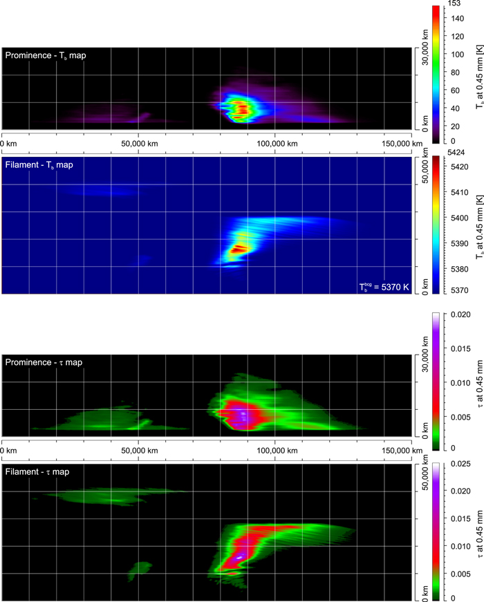
Figure 1. Visualization of the 3D WPFS model at a wavelength of 0.45 mm (666 GHz). Individual panels show, from the top: map of brightness temperature for the prominence view; map of brightness temperature for the filament view; map of optical thickness for the prominence view; map of optical thickness for the filament view. Displayed color scales are unique for each panel. The value of the background brightness temperature  is indicated in the second panel.
Download figure:
Standard image High-resolution imageThe maps of τ at all selected SMM wavelengths are very similar to each other for both the prominence and the filament views (see bottom two panels of Figures 1–4). They are also similar to the maps of τ for the Hα line center (bottom two panels in Figure 5). On the other hand, the maps of the brightness temperature of the prominence and that of the filament differ significantly between individual wavelengths (top two panels of Figures 1–4).
At 0.45 mm (Figure 1) the modeled prominence is optically thin (τmax ≃ 0.025). The Tb maps of both the prominence and filament reveal a number of easily discernible fine structures that appear as isolated areas with the highest brightness temperature. These areas coincide with locations of the largest values of τ and correspond to the cool and dense prominence plasma located in the deep magnetic dips (see discussion in Gunár & Mackay 2016).
At 1.25 mm (Figure 2) the fine structures in the Tb map of the prominence appear very similar to those at 0.45 mm (Figure 1). Individual horizontal fine structures—corresponding to the coolest and densest plasma—are still clearly visible. However, in the filament view (second panel of Figure 2) a split in the elongated fine structures becomes visible. Compared to the continuous regions of the highest Tb visible in Figure 1 (second panel) only the peripheral parts are now very bright. The central parts of these structures now have a considerably lower Tb. These central parts coincide with the regions of the greatest optical thickness, which suggests that the lower  at their location is caused by absorption of the background radiation. On considering the values of τ it might be surprising that values of about 0.1 (see bottom panel of Figure 2) could cause such a significant effect. However, values of τ ≃ 0.1 correspond to a reduction in the background brightness temperature
  by approximately 10%. In our case that corresponds to a decrease in the brightness temperature by approximately 630 K. Such a decrease is comparable to the values of the maximum brightness temperature produced by the prominence plasma itself—around 700 K—which can be estimated from the prominence view (see top panel of Figure 2). Thus the resulting Tb at the location with τ ≃ 0.1 is similar to
  . If, as in this case, the geometrical extent of the area with the highest τ is smaller than the extent of the area with the highest Tb, then the peripheral parts of such elongated areas are not strongly affected by the absorption of the background radiation. As a consequence they appear brighter than the central part, which is affected by the absorption.
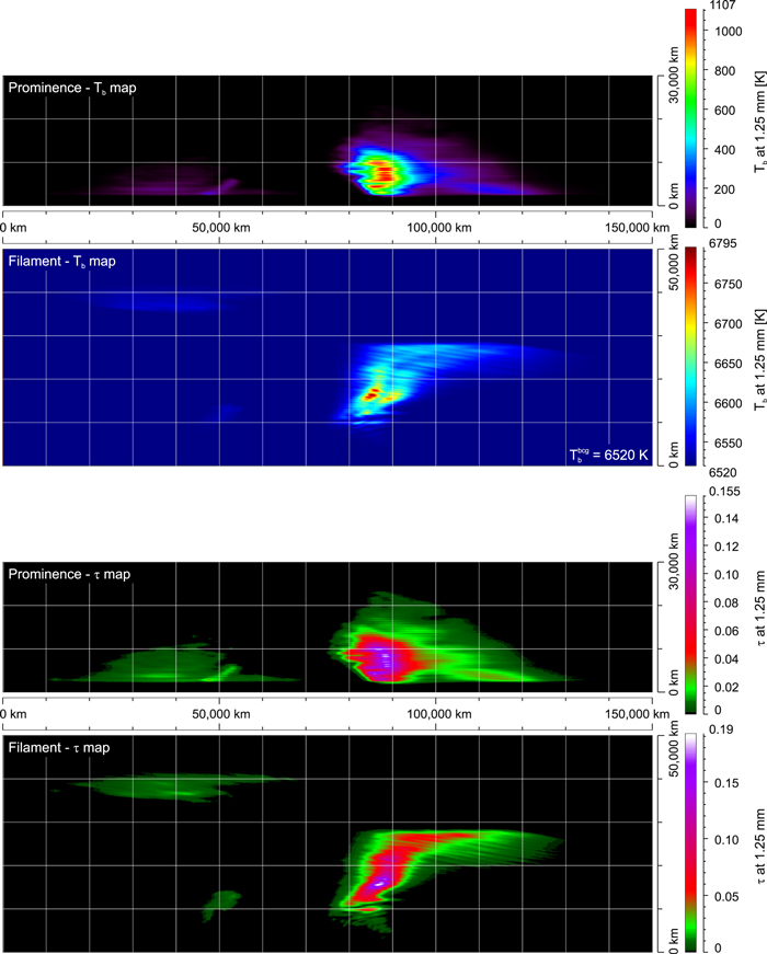
Figure 2. Visualization of the 3D WPFS model at a wavelength of 1.25 mm (240 GHz). Individual panels show, from the top: map of brightness temperature for the prominence view; map of brightness temperature for the filament view; map of optical thickness for the prominence view; map of optical thickness for the filament view. Displayed color scales are unique for each panel. The value of the background brightness temperature  is indicated in the second panel.
Download figure:
Standard image High-resolution imageThis effect is even more pronounced at a wavelength of 3.0 mm (Figure 3). Here, for the filament case the maximum optical thickness exceeds unity (see bottom panel of Figure 3). This results in a strongly visible region of low Tb, which splits the brightest part of the filament into two (see the second panel of Figure 3). There is no equivalent split in the prominence view (top panel of Figure 3), where the horizontal fine structures (areas with the highest Tb) remain similar to those at the previous wavelengths. The horizontal fine structures in the prominence view are still easily discernible and significantly better constrained then those visible in the Hα line. The brightness temperature values in the prominence view do not yet directly correspond to the kinetic temperature of the modeled prominence plasma because the optical thickness does not exceed unity.

Figure 3. Visualization of the 3D WPFS model at a wavelength of 3.0 mm (100 GHz). Individual panels show, from the top: map of brightness temperature for the prominence view; map of brightness temperature for the filament view; map of optical thickness for the prominence view; map of optical thickness for the filament view. Displayed color scales are unique for each panel. The value of the background brightness temperature  is indicated in the second panel.
Download figure:
Standard image High-resolution imageThe situation is different at a wavelength of 9.0 mm, where τ is significantly larger. Here the values of Tb represent a reasonably good estimate of the kinetic temperature of the modeled prominence plasma at depths where τ is around unity (see discussion in Section 5.1). The structures visible in the Tb map of the prominence view are now significantly different from those seen at shorter wavelengths. We no longer see individual horizontal fine structures. The areas with the highest Tb are now more continuous and form a vertically oriented, larger prominence structure. This structure is similar to that visible in the synthetic Hα image (Figure 5). On the other hand, in the filament view the structures visible at 9.0 mm and in the Hα line are significantly different. While in the Hα line we see the whole structure of the modeled filament in absorption, at 9.0 mm only the central part is in absorption (has low Tb). This part of the filament coincides with the area of the highest τ (see second panel of Figure 4). Areas of high Tb are divided into two parts, similar to what was found at shorter wavelengths.
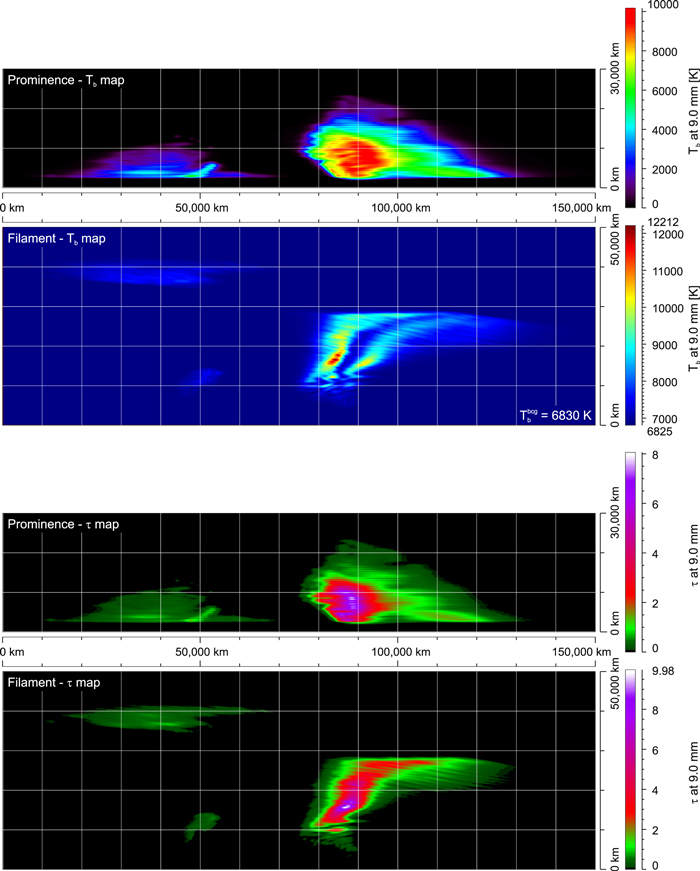
Figure 4. Visualization of the 3D WPFS model at a wavelength of 9.0 mm (33 GHz). Individual panels show, from the top: map of brightness temperature for the prominence view; map of brightness temperature for the filament view; map of optical thickness for the prominence view; map of optical thickness for the filament view. Displayed color scales are unique for each panel. The value of the background brightness temperature  is indicated in the second panel.
Download figure:
Standard image High-resolution image5. DISCUSSION
The results of the present paper (Figures 1–5) clearly demonstrate the ability of ALMA to provide observations of prominences spanning both optically thin and thick regimes. The optical thickness in the modeled prominence ranges from very low values at a wavelength of 0.45 mm (τmax ≃ 0.025) to rather large (τmax ≃ 10.0) at 9.0 mm. This is consistent with the results of Heinzel et al. (2015a), even though it uses a different approach. The optical thickness at 9.0 mm already exceeds the Hα optical thickness. ALMA will have the ability to span both regimes of optical thickness in prominences during its Cycle 4—the first regular solar observing cycle—in which data from band 3 (covering a wavelength of 3.0 mm) and band 6 (covering 1.25 mm) will be available. This range is demonstrated by results shown in Figures 2 and 3. The synthetic maps of the brightness temperature presented in the current paper show an interesting difference in the appearance of the fine structures between the prominence and filament views. This difference is most visible in Figures 2 and 3, where fine structures in the prominence view appear as elongated horizontal threads. These represent parts of the magnetic dips filled with the cool and dense prominence plasma (see, e.g., Gunár et al. 2013b) and correspond to the fine structures visualized in the Hα line in Heinzel et al. (2015b). On the other hand, in the filament view we see the bright regions of Tb divided by an area of lower Tb. This is caused be a partial absorption of the background radiation, as we discuss in Section 4.

Figure 5. Visualization of the 3D WPFS model at the Hα line center. Individual panels show, from the top: synthetic intensity of Hα line center in the prominence view; synthetic intensity of Hα line center in the filament view; map of optical thickness for the prominence view; map of optical thickness for the filament view. Displayed color scales are unique for each panel. This figure is adapted from Gunár & Mackay (2015b).
Download figure:
Standard image High-resolution image
Significant differences in the appearance of prominence fine structures when observed at the limb and on the disk are well documented (see, e.g., Gunár et al. 2013a). However, a considerable difference exists between the extent of the absorbing areas at ALMA wavelengths—only the central parts are dark (in absorption) while the peripheral parts appear bright (in emission)—and in the Hα line, where the whole filament is in absorption. Such differences may help us to better understand the nature of the prominence fine structures. They also highlight the importance of access to simultaneous observations of prominences in the full ALMA range, together with complementary observations in the optical range. Without such a broad range of observations it might be difficult to correctly interpret ALMA observations of prominences and filaments. This can be illustrated with the results shown in, e.g., Figure 3. If such an observation of a filament were obtained only at a wavelength of 3.0 mm at a given time—as will be the case during Cycle 4 when two bands will be available, but not on the same day—it would be difficult to decide whether the observed areas of bright Tb represent individual plasma fine structures or whether there is a region of even denser plasma located between these bright areas that absorbs the background radiation. It should be noted here that only observations of a filament or a prominence can be obtained at a given time. Views of both that help us to understand the nature of the fine structures visible in the maps of brightness temperature can be provided only by 3D models.
In future, ALMA will provide high-resolution observations of prominences obtained simultaneously and co-spatially in both optically thin and thick regimes. Such observations could provide answers regarding the composition of the often observed quasi-vertical threads of prominence fine structures. It is not yet clear if such threads are composed of a series of small-scale plasma structures located in quasi-vertically aligned magnetic dips or caused by some other mechanism. The quasi-vertical propagation of the magnetic dips, owing to the deformation of the field, which is caused by the weight of the plasma loaded in individual dips, was assumed by Heinzel & Anzer (2001), who modeled the vertical prominence fine structures as 2D vertically infinite threads. Such 2D models can produce synthetic hydrogen spectra in very good agreement with observations. This was shown by, for example, Gunár et al. (2008, 2010, 2012), Berlicki et al. (2011), or Schwartz et al. (2015). The mechanism for the production of the gravity-induced vertical propagation of the plasma-filled magnetic dips was studied by Hillier & van Ballegooijen (2013).
5.1. Relationship between Brightness and Kinetic Temperatures
For the case of observations at two different SMM wavelengths, where the prominence plasma is optically thin at one wavelength but optically thick at the other, the kinetic temperature can be derived from the ratio of the obtained brightness temperatures (see, e.g., Heinzel et al. 2015a). An example of such a case is the combination of the wavelengths of 1.25 mm and 3.0 mm shown here (Figures 2 and 3). The kinetic temperature derived from such an approach represents an average of the actual kinetic temperature distribution along the given LOS, where it is weighted by the distribution of the optical thickness along that LOS. In future, we will use the maps of brightness temperature provided by the 3D WPFS model to analyze the difference between the kinetic temperature derived by the ratio-comparison method and the actual kinetic temperature provided by the model.
In the optically thick case (such as that shown in Figure 4) the brightness temperature saturates to the value of the kinetic temperature at a depth around τ = 1 (see, e.g., Heinzel et al. 2015a). However, the kinetic temperature at the depth of τ = 1 might not necessarily be the lowest temperature present in a given prominence. For example, the depth of τ = 1 might be encountered within a prominence fine structure that does not have the minimum temperature, or at a location where the kinetic temperature begins to rise toward the values in the prominence–corona transition region (PCTR). This might be the case in the Tb maps obtained at a wavelength of 9.0 mm presented here (Figure 4). In the prominence view (top panel of Figure 4) we see that the brightest areas have a brightness temperature of up to 10,000 K. As the optical thickness exceeds unity (see the third panel of Figure 4) the obtained Tb values correspond to the kinetic temperature at a depth of around τ = 1. However, in the WPFS model the minimum kinetic temperature in the center of all modeled fine structures is set to be 7000 K (see Gunár & Mackay 2015a). Therefore, we have obtained the brightness temperature that corresponds to the kinetic temperature at the location where the temperature begins to rise. In general, this means that the brightness temperature obtained from observations at wavelengths where τ exceeds unity may correspond either to the minimum kinetic temperature of the observed plasma or to the kinetic temperature above the temperature minimum. The observed brightness temperature thus represents the upper limit of the minimum kinetic temperature of the observed plasma.
Another interesting point to note is the actual link between the brightness and kinetic temperatures in optically thin conditions. From Equation (8) it could be assumed that in the optically thin limit the brightness temperature is directly proportional to the kinetic temperature ( ). In fact, the absorption coefficient κν is proportional to T−3/2 (see Equation (5)). This means that the brightness temperature is actually inversely proportional to the square root of the kinetic temperature (
 )—see, e.g., Equation (11) of Heinzel et al. (2015a) and the discussion therein. This means that the brightness temperature should decrease with increasing kinetic temperature. This is suggested also by the synthetic Tb maps presented in this paper (see Figures 1–4). The brightness temperature in areas where the optical thickness is low decreases from the maximum Tb values located in the central parts of the modeled prominence. In contrast, from the WPFS model it is clear that the kinetic temperature increases from the central cool parts of the modeled prominence toward the boundaries of the modeled prominence fine structures (see Gunár & Mackay 2016). Such a relationship between the brightness and kinetic temperatures might have a significant effect on the derivation of the kinetic temperature of an observed prominence from the obtained maps of brightness temperature. We will study this effect in detail in future.
6. CONCLUSIONS
ALMA will provide unique opportunities for broadening our understanding of solar prominences. It will observe prominences and filaments with a very high spatial resolution. Importantly, ALMA will provide high-resolution observations in both the optically thin and optically thick regimes. Initially, prominences at the limb and on the disk will not be observed at different wavelengths (frequencies) simultaneously. However, when the full capabilities of ALMA become available for solar observations, simultaneous—and thus also co-spatial—observations should be possible.
In addition to the information about the spatial distribution of the plasma in prominences, ALMA will provide maps of the brightness temperature in a broad range of wavelengths. These Tb maps can be interpreted in terms of the kinetic temperature of the observed prominence plasma. This will help us to answer the question of the energy balance of prominences, for which the temperature of the cool prominence core is a critical parameter (see, e.g., Heinzel et al. 2014). Moreover, the high-resolution information about the temperature distribution of the prominence plasma will be instrumental in studies of the PCTR—the transition region between the cool prominence plasma and the hot corona. It is still an open question as to whether the PCTR is distributed around individual prominence fine structures or is a global region surrounding entire prominences, or a combination of the two (see, e.g., discussion in Gunár et al. 2014).
As we demonstrate in the present paper, such a broad range of simultaneous observations would be essential for revealing new information about the nature of the prominence fine structures. Observations at wavelengths where prominences both at the limb and on the disk are optically very thin—such as those at 0.45 mm (666 GHz) in band 9 (see Figure 1)—will provide a view on filaments without the effect of the absorption seen at longer wavelengths (see Figure 2 or 3). Such an unaffected view will be important for the correct interpretation of filament observations at wavelengths where the optical thickness increases. On the other hand, observations at wavelengths where both prominence and filament fine structures have an optical thickness exceeding unity—for example at 9.0 mm (33 GHz) possibly within band 1 (see Figure 4)—will provide us with information about the kinetic temperature of the prominence plasma at depths of around τ = 1.
We also show that prominence modeling will be important for understanding the links between the prominence fine structures observed by ALMA at the limb and on the disk. Complex 3D prominence models providing realistic distributions of the prominence plasma and magnetic field (such as those of Gunár & Mackay 2015a) could also be instrumental in understanding the relations between the observed brightness temperature (at various wavelengths), the mean kinetic temperature derived from observations, and the actual kinetic temperature of the prominence plasma.
S.G. and P.H. acknowledge the support from grant 16-17586S of the Czech Science Foundation (GAČR). S.G. acknowledges support from the European Commission via the Marie Curie Actions—Intra-European Fellowships Project No. 328138. S.G. and P.H. acknowledge the support from project RVO:67985815 of the Astronomical Institute of the Czech Academy of Sciences. The work of P.H. was supported by the Royal Society of Edinburgh. S.G. and P.H. are grateful for the support from the MPA Garching. U.A. is grateful for the support from the Astronomical Institute of the Czech Academy of Sciences. D.H.M. acknowledges financial support from the STFC, the Leverhulme Trust, and NASA. ALMA is an international partnership of the European Southern Observatory (ESO), the U.S. National Science Foundation (NSF), and the National Institutes of Natural Sciences (NINS) of Japan, together with NRC (Canada), NSC and ASIAA (Taiwan), and KASI (Republic of Korea), in cooperation with the Republic of Chile. S.G. is an expert member of the Solar Simulations for the Atacama Large Millimeter Observatory (SSALMON) network.