


Abstract
USNO-B1.0 1421-0485411 is an eclipsing binary system newly discovered in the Yunnan-Hong Kong wide-field photometric survey. Its orbital period is 1.295 days. Based on the V- and R-band photometric data collected at Kunming 1.0 m telescope and spectroscopic data observed at Lijiang 2.4 m telescope, we used the Wilson-Devinney program to determine the physical parameters of the binary system. The results show that the mass and radius are 2.21 M⊙ and 1.70 R⊙ for the A0V primary component, and 2.11 M⊙ and 1.77 R⊙ for the A4–5V secondary one. The observed light curves show higher shoulders around the secondary eclipse, which can originate from hot spots, circumstellar materials, abnormal albedo of the secondary component, etc. Through analyzing and modeling, a quite large albedo (∼1.89) of the secondary component was considered to be the most possible reason for this phenomenon. The position of the two components on the H-R diagram implies that the binary is in main-sequence stage.
Export citation and abstract BibTeX RIS

Original content from this work may be used under the terms of the Creative Commons Attribution 4.0 licence. Any further distribution of this work must maintain attribution to the author(s) and the title of the work, journal citation and DOI.
1. Introduction
The well-determined stellar parameters (especially mass, radius, and age) are the base of stellar structure and evolution research; the bridge between observations and models. Under this background, to determine the stellar parameters precisely is extremely important for stellar physics. Generally, for stars without significant activities, multicolor photometric observations give us the chance to get an estimation of some physical parameters (effective temperature, surface gravity, and metallicity) of the observed stars (Collier Cameron et al. 2007; Majewski et al. 2017; Andrae et al. 2018 ). Moreover the recent space missions make the asteroseismology possible for some stars, which permits to measure the stellar mass and radius (Chen et al. 2017).
On the other hand, the binary systems play one of the most important roles in measuring stellar parameters (Popper 1980; Andersen 1991) because they provide us with more information to measure stellar parameters than single stars due to the orbital motions and eclipsing geometry. However, the proximity effects and material exchanges caused by the interactions between binary components hinder the precise parameter measurements for the semidetached and contact eclipsing binaries. Fortunately, the interactions between components of the detached binaries are quite weak. These relatively simple eclipsing systems can be well modeled and they are the most ideal systems that permit us to get reliable parameter measurements from the observations. Using photometric and spectroscopic data, one can get precise estimation for the stellar parameters of the detached binaries (Wilson 1979; Hill 1989). These reliably determined parameters could be used to constrain the stellar model. For example, such measurements can be regarded as the "candles" to construct a set of reliable set of masses and radii for main-sequence stars (Andersen 1991).
In the beginning of the last century, Russell (1912a, 1912b) derived a general solution for orbital elements of a eclipsing binary based on its photometric light curve. Later, Russell & Merrill (1952) proposed a "mathematical" model for the light curve of an eclipsing binary, which had extended the shape of the components to ellipsoids. After the works of Kopal (1959) and Lucy (1968a, 1968b), Hill & Hutchings (1970) and Wilson & Devinney (1971) developed the methods based on "physical" models to solve the light curve of the eclipsing binary. In the following years, Wilson and Devinney's program (WD code) was developed in many aspects; it included modeling a radial-velocity curve (Wilson 1979), which can provide the masses and radii of two components simultaneously, employed the Kurucz atmospheric model (Kurucz 1979, 1993). Also, it dealt with multiple reflection in a direct way, utilizing different limb-darkening laws, and had linear and nonlinear gravity-darkening functions with adjustable orders. The options on the dynamic third body, the third light, star spots, and circumstellar material were also consecutively plugged in the program (Wilson 1990, 1993; Van Hamme & Wilson 2003, 2007; Wilson 2008, 2012).
It is well known that the value of albedo of each component is between 0 and 1 for a binary system. However, in the study on detached eclipsing binary SZ Cam (Wilson & Rafert 1981), the authors found that a model with the albedo of the secondary component more than one can represent the observed light curves well. One possible reason for such a phenomenon could result from the irradiation of the secondary component of the system (Tassoul & Tassoul 1982).
USNO-B1.0 1421-0485411 = Gaia DR2 20042442252-48160768 (R.A. 22h14m20s, decl. 52°08'33'', J2000) is newly found to be a detached binary in the Yunnan-Hong Kong wide-field photometric survey (hereafter the YNHK survey, which will be published elsewhere). In this paper, we present the first solution of its physical parameters by means of the WD code. The observations and data reduction are given in Section 2. In Section 3, we analyze the light curves and radial-velocity curves and derive its physical parameters. At last, we discuss the results and draw conclusions in Section 4.
2. Observations and Data Reduction
2.1. Survey Detection
The YNHK survey employs an 18 inch main focus Centurion telescope with a correction lens and a 4K × 4K CCD camera, providing a field of view of about 1 7 × 17. During the survey observation, a clear filter is used. USNO-B1.0 1421-0485411 was discovered as a new binary system in one of the survey sky areas, Figure 1 shows one small part of a normal observed CCD image with USNO-B1.0 1421-0485411 inside. The data reduction was performed by using a pipeline that was developed by our group based on PYRAF, the python interface of IRAF package. The result of aperture photometry was reduced to remove systematic errors, and then the magnitude calibration was carried out based on USNO-B1.0 catalog (Huang et al. 2021). The light curve of USNO-B1.0 1421-0485411 obtained from 2016–2017 survey data is shown in Figure 2.
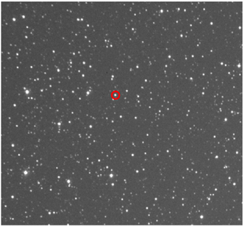
Figure 1. The partial observed image with USNO-B1.0 1421-0485411 inside the red circle.
Download figure:
Standard image High-resolution image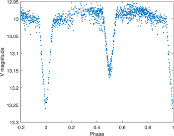
Figure 2. The light curve of USNO-B1.0 1421-0485411 from the survey data.
Download figure:
Standard image High-resolution image2.2. Follow-up Observations
In order to characterize this new binary system, the follow-up photometric observations were carried out from 2018 November 14 to 18 and from December 23 to 27, with the 1 m telescope of Yunnan Observatories. The telescope is located at the headquarter of Yunnan Observatories, which has an altitude of 2000 m. The observations in 2018 November employed a 4K × 4K CCD camera while the observations in 2018 December a 2K × 2K CCD camera, Cousins R and Johnson V filters were used. The weather during the observations was relatively good. The exposure times were 150 s for the R band and 180 s for the V band according to the weather condition and lunar phase. Table 1 lists the detailed information on photometric observations. The reduction of these follow-up photometric data were performed by using a dedicated pipeline developed based on IRAF package at Yunnan Observatories.
Table 1. Information of Follow-up Photometric Observations
| Date | CCD Type | R Image Number | R Exp-time (s) | V Image Number | V Exp-time (s) |
|---|---|---|---|---|---|
| 2018 Nov 14 | 4K × 4K | 18 | 150 | 17 | 180 |
| 2018 Nov 15 | 4K × 4K | 42 | 150 | 44 | 180 |
| 2018 Nov 16 | 4K × 4K | 45 | 150 | 46 | 180 |
| 2018 Nov 17 | 4K × 4K | 47 | 150 | 47 | 180 |
| 2018 Nov 18 | 4K × 4K | 45 | 150 | 46 | 180 |
| 2018 Dec 23 | 2K × 2K | 37 | 150 | 37 | 180 |
| 2018 Dec 24 | 2K × 2K | 35 | 150 | 35 | 180 |
| 2018 Dec 25 | 2K × 2K | 37 | 150 | 37 | 180 |
| 2018 Dec 26 | 2K × 2K | 41 | 150 | 41 | 180 |
| 2018 Dec 27 | 2K × 2K | 40 | 150 | 40 | 180 |
Download table as: ASCIITypeset image
Compared to the photometric observations, the time baseline of the spectroscopic observations was a little longer: 2017 December 14, from 2018 November 13 to 16, and from 2018 December 20 to 24. Fifteen spectra were obtained with the YFOSC instrument of the Lijiang 2.4 m telescope of Yunnan Observatories (Fan et al. 2015; Wang et al. 2019). The telescope is located in Lijiang station with the altitude of 3193 m. Very limited influence of the weather was found during the spectroscopic observations. The general information of the observations is in Table 2. The spectroscopic data were reduced by using a dedicated pipeline developed based on the IRAF package. The procedures include image trimming, bias subtraction, flat-field correction, cosmic ray removal, scatter light subtraction, spectral extraction, and wavelength calibration. To get the normalized spectra, the continuum fitting was done by using a polynomial.
Table 2. Information of Follow-up Spectroscopic Observations Including the S/Ns of Hydrogen Lines
| Date | Exposure Time (s) | Phase | H
| Hγ | Hα |
|---|---|---|---|---|---|
| 2017 Dec 14 | 1200 | 0.357 | 32 | 49 | 54 |
| 2018 Nov 13 | 1800 | 0.209 | 42 | 62 | 60 |
| 2018 Nov 13 | 1800 | 0.307 | 46 | 67 | 56 |
| 2018 Nov 15 | 1800 | 0.750 | 51 | 76 | 77 |
| 2018 Nov 15 | 1800 | 0.802 | 37 | 57 | 63 |
| 2018 Nov 15 | 1800 | 0.849 | 41 | 61 | 55 |
| 2018 Nov 16 | 1800 | 0.521 | 25 | 38 | 35 |
| 2018 Nov 16 | 1800 | 0.567 | 32 | 50 | 54 |
| 2018 Nov 16 | 1800 | 0.638 | 27 | 44 | 57 |
| 2018 Dec 20 | 1800 | 0.780 | 53 | 76 | 57 |
| 2018 Dec 20 | 1800 | 0.854 | 33 | 57 | 70 |
| 2018 Dec 21 | 1800 | 0.594 | 36 | 54 | 47 |
| 2018 Dec 22 | 1800 | 0.364 | 38 | 63 | 68 |
| 2018 Dec 23 | 1800 | 0.141 | 27 | 46 | 53 |
| 2018 Dec 24 | 1800 | 0.877 | 36 | 54 | 54 |
Download table as: ASCIITypeset image
2.3. Period Determination
To derive the accurate orbital period of the system, an O − C analysis was carried out utilizing the observed light minimum times. From the YNHK survey data during 2016 and 2017, 9 eclipses with relatively complete phase coverage were found, which can distinguish the light minimum time clearly. Two more eclipses were obtained in the photometric follow-up observations. To calculate the precise minimum time of every eclipse, we used Gaussian function to fit the above eclipse events. All of the fitted light minimum times are listed in Table 3, where the epochs are the Heliocentric Julian Day (HJD) minus 2,450,000.
Table 3. The Light Minimum Times
| Minimum time | O − C | Cycle |
|---|---|---|
| (HJD 2,450,000+) | (days) | |
| 8409.1953 | 0.0003 | 0 |
| 8411.1369 | −0.0007 | 3 |
| 8413.0806 | 0.0005 | 6 |
| 8435.0970 | 0.0011 | 40 |
| 8437.0381 | −0.0004 | 43 |
| 8795.1188 | 0.0000 | 596 |
| 8806.1281 | 0.0015 | 613 |
| 8817.1336 | −0.0009 | 630 |
| 8819.0767 | −0.0005 | 633 |
| 8437.0379 | −0.0006 | 43 |
| 8437.0384 | −0.0001 | 43 |
Download table as: ASCIITypeset image
Through the O − C analysis, the ephemeris formula was derived as follows:

2.4. Radial-velocity Measurements
With normalized spectra mentioned above, we tried to get the radial-velocity curves of the binary. During the analysis, one spectrum with the phase very near 0.5 was excluded due to difficult to separate the individual profile of the component. Because the rotational velocities of two components are quite large, their profiles are very wide and overlapped together (see Figure 3). Only the hydrogen lines can be easily identified in the spectra and the Hα line is the one showed the strongest double peak structure and had relatively high signal-to-noise ratio (S/N). Therefore, we used two Gaussian/Lorenz functions to fit the Hα lines of each spectrum so as to make individual measurement for the profile of each component, and then calculated the radial velocity by the wavelength shift value. The S/N of the three hydrogen lines in different wavelengths, in which we could find double peak structure, is shown in Table 2. To derive the orbital phase, the corresponding HJD was calculated by the program provided by Eastman et al. (2010). Hydrogen line at the blue side like the H has lower S/N and shows a weak double peak structure, so not suitable for radial-velocity measurement. The Hγ line has a comparable S/N to that of the Hα line but it shows very weak double peak structure, it was also excluded when calculating the radial velocity. We fitted the Hα two peak structure by using IRAF task and the first fitting function was the Gaussian function, after checking the quality of the fitting, an extra fitting by using the Lorenz function was carried out. Through comparison, the better one was adopted as the final result. Based on two central wavelengths of Hα lines for each spectrum, we calculated the radial velocities of two components after considering the motion of the Earth (Hutchings 1973), see Table 4. And the barycentric correction was done by using the code provided by Wright & Eastman (2014). From Figure 2, it is clear that the secondary eclipse is exactly at phase 0.5, which implies the orbit of the binary system to be circular. Based on above radial-velocity measurements, we used two sine functions to fit them under the condition that the orbital eccentricity e = 0. For the two components, we got the semiamplitudes of their radial-velocity curves as K1 = 150.60 km s−1 and K2 = 158.39 km s−1, respectively, which results in a mass ratio (q = m2/m1) of 0.96 for the binary system. If assuming the orbital inclination is 7648, which is from the orbital solution in next section, the masses of two components were estimated as 2.21 M⊙ and 2.10 M⊙ by means of the formula given by Torres et al. (2010).
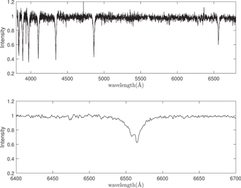
Figure 3. Observed spectrum at phase 0.521 and Hα lines of the binary at phase 0.750.
Download figure:
Standard image High-resolution imageTable 4. The Radial Velocities Measured by Fitting Hα Lines
| Phase | RV 1 (km s−1) | RV 2 (km s−1) |
|---|---|---|
| 0.141 | −174.035 | 80.403 |
| 0.209 | −195.840 | 100.624 |
| 0.307 | −220.721 | 78.483 |
| 0.357 | −190.511 | 66.668 |
| 0.364 | −175.368 | 61.712 |
| 0.567 | −2.870 | −108.391 |
| 0.594 | 21.090 | −147.926 |
| 0.638 | 48.155 | −181.160 |
| 0.750 | 91.079 | −218.632 |
| 0.780 | 85.151 | −204.461 |
| 0.802 | 83.651 | −204.134 |
| 0.849 | 42.900 | −182.760 |
| 0.854 | 44.850 | −184.921 |
| 0.877 | 69.463 | −196.396 |
Download table as: ASCIITypeset image
3. Orbital Solution
Before the procedure to calculate the orbital elements of USNO-B1.0 1421-0485411, it is necessary to get good initial values for some parameters of the binary, which will ensure a reliable result. First of all, we estimated the effective temperature of the primary component. One way is using the relationship between spectral type and effective temperature (Gray 1976); the spectral type of our target can be inferred from its observed spectra. It is well known that the observed spectra of a binary system are normally the combination of two resources from two components. However, the spectra taken around the secondary eclipse (close to the phase 0.5) can be used to represent the one of the primary star because it plays a more important role in the mixed spectra (see Figure 3). Compared with the typical stellar spectra (Gray & Christopher 2009), our target's spectrum shows a series of strong hydrogen lines, very weak metal lines, and very weak He lines; these characters imply it is an A- or B-type star. For most A type stars, Ca ii K line is very strong, only the A0 type spectrum shows Ca ii K line with the similar depth to our targets spectrum. On the other hand, most B-type stars show distinct He lines at the wavelength of 4009 and 4026 Å; however, these lines are very weak in all of our spectra and cannot be identified in some of our observed spectra, only the B9 type spectrum shows the similar character to our observed spectra. So, our target can be classified as an A0 or B9 star. In addition, we used Grays code MKCLASS (Gray & Corbally 2014) to do classification, the result showed that the target is an A0 type star, which is quite consistent with above analysis. Gaia DR2 (Gaia Collaboration et al. 2018) gave the effective temperature of 9572 K to our target, which is compatible to an A0V type star, thus the effective temperature (T1) of the primary star was set to 9572 K and fixed during the calculation.
The gravity-darkening coefficients (g1, g2) were set as the typical value 1.0 because of our target is with radiation envelop (Claret 2003). While the limb-darkening coefficients (×1, ×2) were from a table provided by WD code, the code automatically gets the limb-darkening coefficients from the table according to the stellar parameters. The albedo (A1, A2) for the two components was set to 1.0 for early-type stars as usual (Rafert & Twigg 1980). According to Zahn (1966, 1975, 2008), Lubow & Shu (1975), Hut (1981), Tassoul (1988), Zahn & Bouchet (1989), and Goldreich & Nicholson (1989), for the case that the orbital angular momentum is larger than the rotational angular momentum, like detached binaries, the rotation synchronization is often faster than orbital circularization. Furthermore, for the binaries with shorter orbital periods (<7 days), their orbits are considered to be circular. Because our target's orbital period is 1.295 days and the secondary eclipse is at orbital phase 0.5, it is reasonable to assume that our target has a circular orbit and is synchronously rotating.
Based on the shape of light curves, we adopted the mode 2 of WD code, namely the detached mode, to run the DC routine to search the best solution for the follow-up light curves and radial-velocity data. In the course of calculations, the parameters T1, g1, g2, x1, x2, A1, A2, and q were fixed as the values mentioned above, the orbital inclination i, the effective temperature T2 of the secondary component, the surface potentials Ω1 and Ω2 of two components and the luminosity L1 of the primary component were free parameters. After we got the initial converged solution, the mass ratio q was also changed to be a free parameter. Through plenty of differential correction calculations, the solution was converged (hereafter solution 1) and the values of parameters were derived, which were input to the LC routine to produce the theoretical light curves in Figure 4 (green curves). It can be found the model can reproduce the observing light curves well, except the shoulders of the secondary eclipse, which implies that there exist some other physical mechanisms that were not included in above modeling. Through the comparison between the model and observations in Figure 4, two instant imaginings are either there are hot spots in the system or the secondary component should have a large albedo. So we decided to simulate these two possible cases by means of WD code in the next step.
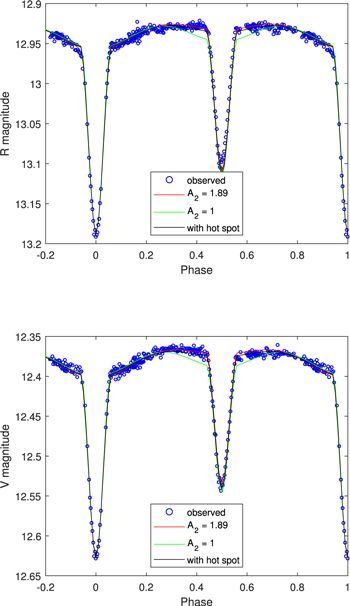
Figure 4. The observing light curves and models with A2 = 1.886 and a hot spot on the secondary component.
Download figure:
Standard image High-resolution imageFirst, we considered that the secondary component has a large albedo, which means that there exists irradiation on the secondary component of the system. The whole procedure was almost the same as above solution 1, except A2 was also set to be a free parameter. We ran the DC routine again through the iterations of differential correction until a converged solution was obtained (hereafter solution 2), and the result demonstrated that the albedo of the secondary component A2 = 1.89, which is quite large comparing with the theoretical value. Based on this solution, the observed light curves in V and R bands are reproduced very well (see Figure 4, red curves), while modeling of the radial-velocity curves is shown in Figure 5 (red curves). Second, based on the solution 1, we tried to add hot spots on the primary component or secondary one or both of them to perform DC calculations, respectively, so as to reproduce the higher shoulders of the secondary eclipse. After a number of DC iterations, the converged results were derived for three situations, and the results demonstrate that the solution with a hot spot on the secondary component has the minimum fitting residual, which implies this is the favorite solution for the hot-spot model. Hereafter we denote it as solution 3, the corresponding theoretical light curves calculated by using LC routine are also plotted in Figure 4 (black curves). The system parameters from the best orbital solutions for the above two cases (solution 2 and 3) are listed in Table 5, where "Fixed" means the parameter was not adjusted during the DC calculation, a is the orbital semimajor axis, Vγ is the radial velocity of the binary barycenter, Ωin is the potential of the inner critical equipotential surface of the binary, L1 and L2 are the absolute luminosity of the two components, r1 and r2 are relative radii of two components, R1 and R2 are the absolute radii of the two components, M1 and M2 are the absolute masses of the two components, log g1 and log g2 are their surface gravities, Latspot, Lonspot, Rspot, and Tspot/Tpho are the latitude, longitude, radius of the hot spot, and the temperature ratio between the hot spot and the photosphere, respectively. Because the range of T1 was provided by Gaia DR2, we tried to estimate the errors of other parameters by applying the approximate error of T1, the errors of other parameters were calculated through three DC calculations (with T1 of 9512, 9572 and 9613 K). The error of every parameter is from two sources: the deviation of the parameter among the three calculations and the standard deviation provided by WD code. The standard deviation provided by the WD code is only used when it is equivalent to or larger than the deviation among the three calculations. In addition, the errors of some physical parameters were acquired by the error propagation analysis.
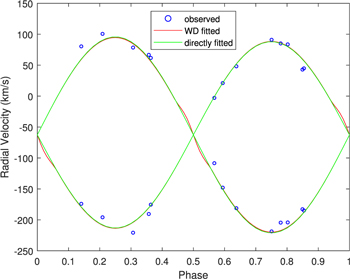
Figure 5. The observing and modeling radial-velocity curves. The red curves represent the results from WD code, and the green ones represent the results from direct fitting of the RVs.
Download figure:
Standard image High-resolution imageTable 5. The Physical Parameters of the Binary
| Solution 2 | Solution 3 | |||
|---|---|---|---|---|
| Parameter | Value | Error | Value | Error |
| a | 8.14 R⊙ | ±0.11 R⊙ | 8.14 R⊙ | ±0.11 R⊙ |
| Vγ | −62.6 km s−1 | ±8.1 km s−1 | −62.6 km s−1 | ±8.1 km s−1 |
| i | 7648 | ±005 | 7648 | ±009 |
| g1 = g2 | 1.0 | Fixed | 1.0 | Fixed |
| T1 | 9572 K | ±60 K | 9572 K | ±60 K |
| T2 | 8472 K | ±58 K | 8404 K | ±63 K |
| A1 | 1.0 | Fixed | 1.0 | Fixed |
| A2 | 1.886 | ±0.086 | 1.0 | Fixed |
| Ω1 | 5.782 | ±0.041 | 5.779 | ±0.037 |
| Ω2 | 5.445 | ±0.031 | 5.462 | ±0.023 |
| Ωin | 3.668 | 3.668 | ||
| q(M2/M1) | 0.955 | ±0.006 | 0.955 | ±0.007 |
| L1/(L1 + L2)V | 0.542 | ±0.018 | 0.571 | ±0.019 |
| L2/(L1 + L2)V | 0.458 | ±0.018 | 0.429 | ±0.019 |
| L1/(L1 + L2)R | 0.528 | ±0.016 | 0.556 | ±0.018 |
| L2/(L1 + L2)R | 0.472 | ±0.016 | 0.444 | ±0.018 |
| x1V | 0.428 | Fixed | 0.428 | Fixed |
| x2V | 0.484 | Fixed | 0.484 | Fixed |
| x1R | 0.359 | Fixed | 0.359 | Fixed |
| x2R | 0.403 | Fixed | 0.403 | Fixed |
| r1(R1/a) | 0.21 | ±0.01 | 0.21 | ±0.01 |
| r2(R2/a) | 0.22 | ±0.01 | 0.22 | ±0.01 |
| K1 | 150.98 km s−1 | ±5.98 km s−1 | 151.19 km s−1 | ±6.05 km s−1 |
| K2 | 157.26 km s−1 | ±6.90 km s−1 | 158.23 km s−1 | ±6.96 km s−1 |
| R1 | 1.70 R⊙ | ±0.08 R⊙ | 1.70 R⊙ | ±0.08 R⊙ |
| R2 | 1.77 R⊙ | ±0.08 R⊙ | 1.76 R⊙ | ±0.08 R⊙ |
| M1 | 2.21 M⊙ | ±0.09 M⊙ | 2.21 M⊙ | ±0.09 M⊙ |
| M2 | 2.11 M⊙ | ±0.09 M⊙ | 2.11 M⊙ | ±0.09 M⊙ |
| L1 | 21.88 L⊙ | ±0.82 L⊙ | 21.68 L⊙ | ±0.81 L⊙ |
| L2 | 14.45 L⊙ | ±0.64 L⊙ | 13.93 L⊙ | ±0.65 L⊙ |
| log g1 | 4.32 | ±0.04 | 4.32 | ±0.04 |
| log g2 | 4.27 | ±0.04 | 4.27 | ±0.04 |
| Latspot | 1.96 rad | ±0.42 | ||
| Lonspot | 0.00 rad | Fixed | ||
| Rspot | 0.72 rad | ±0.15 | ||
| Tspot/Tpho | 1.02 | ±0.01 |
Note. "Fixed" refers to the parameters from prior information that remain fixed during DC calculation.
Download table as: ASCIITypeset image
4. Discussion and Conclusions
We have analyzed the VR light curves and radial-velocity curves of the new identified double-lined eclipsing binary USNO-B1.0 1421-0485411 by means of the widely used WD code, and derived its system parameters. This is a detached system, its configuration is displayed in Figure 6. Based on the spectral classification, the spectral type of the primary component is A0V. According to the WD result T2 = 8472 K, the spectral type of the secondary component can be estimated as A4–A5V. As the radial velocities of each component were measured by fitting the shape of only one line (Hα) of observed spectra using two Gaussian (Lorenz) functions and their S/Ns are not very high, the radial-velocity curves are a little scattered, but still can be employed to constrain the mass ratio of the binary.
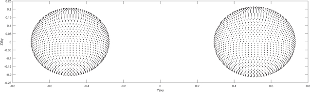
Figure 6. The configuration of the binary system at phase 0.25.
Download figure:
Standard image High-resolution imageFrom Figure 4 it can be seen that the shoulders outside the secondary eclipses are obviously higher than the shoulders outside the primary eclipses. Several reasons could possibly lead to this phenomenon, such as star spots, circumstellar materials, hot spots, the third body, and irradiation of the secondary component. Star spots normally appear on late-type stars. Furthermore, chromospheric emission, which is an evidence for star-spot activity, cannot be found in our observed spectra. For other possibilities, we have modeled two cases, namely hot spot and irradiation on the secondary component, by using the WD code. Although both of the two solutions can well reproduce the observed light distortion around the secondary eclipse, the hot-spot model seems less reasonable because the hot spot should be formed by the accretion of circumstellar materials for a detached binary system, and we cannot see any emission resulting from the impact of the circumstellar materials on the secondary component at the Hα line of the observed spectra. Thus, based on the current observational data, we think a strong irradiation on the secondary component should be the most probable reason for the higher shoulders of the secondary eclipse. To simulate a stronger irradiation on the secondary component, one reasonable way is to permit the albedo of the secondary component larger than one, while keeping that of the primary one at 1. In our case, the converged solution is A2 = 1.886. The large albedo of a star in a specific band can be explained by the energy transfer: star can absorb the energy in a band and reradiates the energy in other bands by changing its surface temperature. Ruciński (1970) analyzed the reflection effect in binaries and indicated that the illuminated atmosphere has a complicated spectral distribution that cannot be predicted by the combination of emergent flux and the unilluminated atmosphere radiation. The monochromatic albedos are wavelength dependent. Wilson & Rafert (1981) used the 1971 version of WD code to do parameter determination of four early-type binary systems. Among them, the SZ Cam had a similar light curve to our target but with flat shoulders outside the primary and secondary eclipses. When letting the albedos of components to be adjustable, a secondary albedo of 1.51 ± 0.60 was reached. Eaton & Shaw (2007) studied 22 Vul and used the spectroscopic and photometric data to constrain its physical properties to investigate the rotation and wind of the chromosphere. While solving the light curves with their program (Eaton & Hall 1979) with constraints derived from the spectra, a 1.59 ± 0.14 bolometric albedo for the cooler G-type star was reached. They attributed this result to the high complexity of the reflection effect. In our case, the two components have similar masses; perhaps their different evolution tracks result in how the secondary component shows irradiation while the primary one does not.
To verify whether our WD solution is unique, we tried to add some deviations to the parameters fixed during the DC calculations, and then followed the same procedure as before to derive the solutions. The results show that we almost got the same solutions; that is, for each parameter, there only exists very small difference between these test solutions and above solution 2. This demonstrates that our WD solution is quite reliable.
To figure out the evolution stage of the two components, we used the theoretical stellar evolution tracks calculated by using Modules for Experiments in Stellar Astrophysics (MESA; Paxton et al. 2011). In Figure 7, the three lines are stellar evolution models of M = 1.9M⊙, M = 2.1M⊙, and M = 2.2M⊙, all of which have the metallicity of [M/H] = 0. These show the evolution tracks of stars in main-sequence stage and the lower-left extremity of every line is the Zero Age Main Sequence (ZAMS) position of each evolution model. It is obvious that both components are in main-sequence stage, noticing that the primary component is located at the M = 2.2M⊙ evolution track and the secondary component is at the M = 1.9M⊙ track. The primary component is very near the ZAMS and the secondary one is also close to the ZAMS. We adopted CMD, a web interface dealing with stellar isochrones and their derivatives based on the tracks of Girardi et al. (2000) and Marigo et al. (2008), to estimate the age of this binary system. Based on the system parameters from the WD solution 2, we drew the two components on the H-R diagram with the isochrones of log(Age) from 8.3 to 8.8 calculated by CMD. As shown in Figure 8, the logarithms of ages of the two components are  for the primary and
  for the secondary. Three possible reasons can result in such a difference. The first one is that the two components were not formed at the same time. The primary was formed later than the secondary and the binary system was formed by the approaching, catching and orbit evolution of the two stars. The second one is the two components were formed at the same time, previous mass exchange made the present difference. The third one is that the primary is a normally evolved young main-sequence star, while the secondary has a larger radius than the theoretical model, and some physical processes make the secondary expand more rapidly.
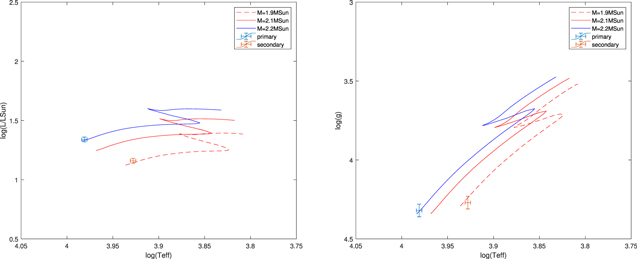
Figure 7. Two components on the H-R and log(Teff)–log(g) diagrams.
Download figure:
Standard image High-resolution image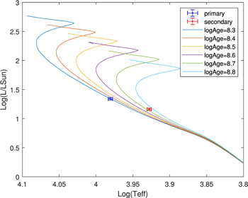
Figure 8. Two components with isochrones in main-sequence stage.
Download figure:
Standard image High-resolution image
In the near future, we shall analyze other detached binary systems discovered in YNHK survey so as to contribute more on stellar basic parameters.
We are very grateful to the referee for the constructive comments, which greatly improved the quality of the paper. We thank the staff of the 2.4 m telescope at the Lijiang station of Yunnan Observatories for their help during our observations. Funding for the 2.4 m telescope has been provided by the Chinese Academy of Sciences and the People's Government of Yunnan Province. We are grateful to Dr. Tao Wu for helping to calculate with the MESA code. This study is supported by the National Natural Science Foundation of China under grants Nos. 10373023, 10773027, U1531121, 11603068, and 11903074.