


Abstract
The legacy of NASA's K2 mission has provided hundreds of transiting exoplanets that can be revisited by new and future facilities for further characterization, with a particular focus on studying the atmospheres of these systems. However, the majority of K2-discovered exoplanets have typical uncertainties on future times of transit within the next decade of greater than 4 hr, making observations less practical for many upcoming facilities. Fortunately, NASA's Transiting Exoplanet Survey Satellite (TESS) mission is reobserving most of the sky, providing the opportunity to update the ephemerides for ∼300 K2 systems. In the second paper of this series, we reanalyze 26 single-planet, K2-discovered systems that were observed in the TESS primary mission by globally fitting their K2 and TESS light curves (including extended mission data where available), along with any archival radial velocity measurements. As a result of the faintness of the K2 sample, 13 systems studied here do not have transits detectable by TESS. In those cases, we refit the K2 light curve and provide updated system parameters. For the 23 systems with M* ≳ 0.6 M⊙, we determine the host star parameters using a combination of Gaia parallaxes, spectral energy distribution fits, and MESA Isochrones and Stellar Tracks stellar evolution models. Given the expectation of future TESS extended missions, efforts like the K2 and TESS Synergy project will ensure the accessibility of transiting planets for future characterization while leading to a self-consistent catalog of stellar and planetary parameters for future population efforts.
Export citation and abstract BibTeX RIS

Original content from this work may be used under the terms of the Creative Commons Attribution 4.0 licence. Any further distribution of this work must maintain attribution to the author(s) and the title of the work, journal citation and DOI.
1. Introduction
The past two decades have been fruitful for exoplanet discovery, with over 5000 exoplanets confirmed to date. 8 While new discoveries are still being made, we are simultaneously venturing into an era of exploring known systems in further detail, with a variety of dedicated efforts for exoplanet characterization. Facilities that are operational or expected to be online in the next decade such as JWST (Gardner et al. 2006; Beichman et al. 2020), the 39 m European Southern Observatory Extremely Large Telescope (ELT; Udry et al. 2014), the Nancy Grace Roman Space Telescope (e.g., Carrión-González 2021), the Giant Magellan Telescope (Johns et al. 2012), and the Atmospheric Remote-sensing Infrared Exoplanet Large-survey (ARIEL; Tinetti et al. 2018, 2021) will provide key information about the atmospheres of exoplanets and insight into their formation and evolutionary processes. However, these ongoing and future endeavors to reobserve known transiting exoplanets heavily rely on precisely knowing the transit time, which is challenged by the degradation of the ephemeris over time.
Most exoplanets and candidates found to date were originally discovered by the Kepler mission (Borucki et al. 2010). Kepler was launched in 2009 with the goal of understanding the demographics of transiting exoplanets. This mission was a success, having discovered ∼2700 confirmed planets with a further ∼2000 candidates, 9 in addition to advancing our understanding of the host stars they orbit (e.g., Bastien et al. 2013; Berger et al. 2020a, 2020b). However, by May of 2013 two of the four reaction wheels on the spacecraft had failed, severely limiting the pointing of Kepler, threatening to end the mission. A solution was conceived to point the spacecraft at the ecliptic to reduce torque from solar radiation pressure, so that the remaining two reaction wheels, along with the thrusters, could maintain sufficient stability. This saw Kepler successfully reborn as the K2 mission (Howell et al. 2014). While Kepler continuously pointed at one region of sky, the necessity of K2 being aimed along the ecliptic opened up an opportunity to study different populations of stars. K2 continued on the path of exoplanet discovery, with currently ∼500 confirmed planets and another ∼1000 candidates found by the time the spacecraft retired in 2018, when fuel for the thrusters ran out (Crossfield et al. 2016; Pope et al. 2016; Vanderburg et al. 2016; Livingston et al. 2018a; Dattilo et al. 2019; Kruse et al. 2019; Zink et al. 2021).
Unfortunately, many of the known planets discovered by the K2 mission have not been reobserved since their discovery, leading to future transit time uncertainties of many hours (Ikwut-Ukwa et al. 2020). This has recently changed with the launch of NASA's Transiting Exoplanet Survey Satellite (TESS) mission in 2018 (Ricker et al. 2015), the successor to the Kepler and K2 missions. The 2 yr primary mission of TESS aimed to observe more than 200,000 stars at 2-minute cadence across ∼75% of the sky. To date, TESS has found ∼280 confirmed planets and another ∼6100 candidates. 10 Even though K2 targeted the ecliptic plane and the TESS primary mission only skimmed the edges of some K2 fields, there are ∼30 systems that were observed by both (single- and multiplanet systems). This provides an opportunity to begin updating the ephemerides and parameters of K2 systems that have been reobserved by TESS. The first extended mission of TESS began during 2020 and includes sectors dedicated to the ecliptic plane, providing more substantial overlap of a further ∼300 systems with the K2 fields 11 (Figure 1). With TESS scheduled to reobserve nearly the entire sky during its extended missions, it will be a useful tool for refreshing the ephemerides of thousands of transiting exoplanets.
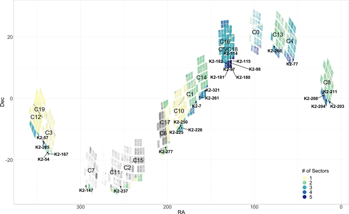
Figure 1. Overlap between K2 campaigns and TESS sectors. The number of times each K2 target was observed in TESS sectors is indicated by the color, with gray indicating no TESS overlap as of Sector 46. The systems analyzed in this study are labeled.
Download figure:
Standard image High-resolution imageCurrently, many known exoplanets do not have sufficiently accurate projected transit times to plan observations with future missions. Even TESS ephemerides will need to be updated, as most TESS planets will have transit time uncertainties exceeding 30 minutes in the era of JWST (Dragomir et al. 2020). With the wealth of data coming from ongoing surveys like TESS and the ability to follow up many planets with small-aperture (<1 m) telescopes (Collins et al. 2018), many efforts have begun to keep the ephemerides of transiting planets from going stale, like the ExoClock Project (Kokori et al. 2021, 2022) for future ARIEL targets and the K2 and TESS Synergy (Ikwut-Ukwa et al. 2020). Ephemeris refinement programs focused on citizen science (Zellem et al. 2019, 2020) and high school students (e.g., ORBYTS; Edwards et al. 2019, 2020, 2021) also provide opportunities to actively engage the public while contributing to an essential aspect of future exoplanet characterization. These efforts will be key to making a large number of systems accessible for future facilities.
A continual renewal of ephemerides also presents an opportunity to create self-consistent catalogs of exoplanets and their parameters, which not only helps to plan for future missions but also allows for appropriate population studies using data that have been uniformly prepared. While the vast amount of data available per system makes this a challenge, the advent of new exoplanet fitting suites to globally analyze large quantities of data, like Juliet (Espinoza et al. 2019), EXOFASTv2 (Eastman et al. 2013, 2019; Eastman 2017), Allesfitter (Günther & Daylan 2021), and exoplanet (Foreman-Mackey et al. 2021), has made it possible to individually model the available observations for a large sample of exoplanetary systems. These types of studies are necessary to uncover large-scale trends or mechanisms that may play important roles in planet formation and evolution. A renowned example is the radius valley of small planets (Fulton et al. 2017), which was achieved through more accurate and consistent handling of host star parameters for over 2000 planets from the California-Kepler Survey.
A case study for updating K2 ephemerides and system parameters with new TESS data was presented in the first paper of this series (Ikwut-Ukwa et al. 2020), where four K2-discovered systems (K2-114, K2-167, K2-237, and K2-261) were reanalyzed by performing global fits using K2 and TESS light curves. This resulted in the uncertainties for the transit times of all four planets being reduced from multiple hours to between 3 and 26 minutes (at a 1σ level) throughout the expected span of the JWST primary mission, showcasing the value of combining the K2 and TESS data. We continue this work by reanalyzing a sample of 26 single-planet systems observed with K2 and the primary TESS mission (including refitting the original four systems for consistency), while also making use of archival radial velocities (RVs), Gaia parallaxes, and any currently available light curves from the TESS extended mission. We focus on previously confirmed single-planet systems, but future papers in this series are expected to reanalyze all K2 systems (including multiplanet systems) as part of an ongoing TESS guest investigator program (G04205, PI Rodriguez). Updated transit times will be made available to the community throughout this series through the Exoplanet Follow-up Observing Program for TESS (ExoFOP). 12
In Section 2 we describe how we obtained and prepared the data used in our global fits. Section 3 outlines how we ran the EXOFASTv2 analysis, and Section 4 presents our results, along with any peculiarities for specific systems. Our conclusions are summarized in Section 5.
2. Observations and Archival Data
Given that most known K2-discovered exoplanet systems will have uncertainties larger than 30 minutes (see Figure 2), we take advantage of the high-quality data obtained with K2 and TESS, simultaneously fitting the photometry and archival spectroscopy to update system parameters for 26 K2 systems. Here we describe the techniques used to obtain and process K2 and TESS light curves, as well as RVs from existing literature.
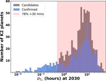
Figure 2. Uncertainty of the transit time ( ) for K2 candidate and confirmed planets at the year 2030, based on the discovery ephemeris. The majority of planets have uncertainties greater than 30 minutes (indicated by the red region) in the era of JWST, making these challenging to reobserve. Values are taken from the NASA Exoplanet Archive (NEA) default parameter sets.
Download figure:
Standard image High-resolution image2.1. K2 Photometry
Each of these stars was observed by the Kepler spacecraft during its K2 extended mission (Howell et al. 2014). During K2, the spacecraft's roll angle drifted significantly owing to the failure of two reaction wheels, which introduced significant systematic errors into its light curves. 13 Over the course of the mission, a number of different techniques and methods were developed to mitigate these errors (e.g., Aigrain et al. 2016; Barros et al. 2016; Luger et al. 2016; Lund et al. 2015; Pope et al. 2019). In this work, we used the methods of Vanderburg & Johnson (2014) and Vanderburg et al. (2016) to derive a rough systematics correction. In brief, these methods involve extracting raw light curves from a series of 20 different photometric apertures, correlating short timescale variations in the raw light curves with the spacecraft's roll angle (which changes rapidly owing to K2's unstable pointing) and subtracting variability correlated with the spacecraft's roll angle. The process of correlating and subtracting variability correlated with the roll angle is performed iteratively until the only remaining variations in the light curve are unrelated to the spacecraft's roll. Finally, we select the aperture that produces the most precise light curve among the 20 originally extracted. Then, we refined the systematics correction by simultaneously fitting the transits for each planet along with the systematics correction and low-frequency stellar variability, prior to the final global fit. Most of the data we analyzed were collected in 30-minute long-cadence data, but when available, we analyzed 1-minute short-cadence exposures for better time sampling. For all systems, we only included out-of-transit data from one full transit duration before and after each transit. This is to optimize the balance between having enough data points to establish the baseline flux of the star and lengthening the runtime of the fits owing to having more data.
2.2. TESS Photometry
While all 26 systems were initially observed by TESS in the primary mission, each was reobserved in at least one sector of the first extended mission. We therefore included TESS light curves from the primary and extended missions up to and including Sector 46 (as of 2022 February 1). This was the final sector dedicated to the ecliptic plane for the first extended mission. Future efforts in this series will analyze systems that were first observed by TESS during the first extended mission and beyond.
We used the Python package Lightkurve (Lightkurve Collaboration et al. 1812) to retrieve TESS light curves from the Mikulski Archive for Space Telescopes (MAST). Three systems within the footprint of the TESS primary mission (K2-42, K2-132/TOI 2643, and K2-267/TOI 2461) did not have corresponding retrievable light curves, which is likely due to being too close to the edge of the detector, so we excluded these from the current analysis. For the TESS light curves, we used the Pre-search Data Conditioned Simple Aperture Photometry (PDCSAP) flux, which is the target flux within the optimal TESS aperture that has been corrected for systematics with the PDC module (Stumpe et al. 2012, 2014; Smith et al. 2012). Typically, observations for each sector are processed through the Science Processing Operations Center (SPOC) pipeline at the NASA Ames Research Center (Jenkins et al. 2016). The SPOC pipeline takes in the raw data and applies corrections for systematics, runs diagnostic tests, and identifies transits, resulting in a calibrated light curve that can be used for analysis.
TESS science observations are taken at 20 s and 2-minute cadences (the former only becoming available from the first extended mission), while the full-frame images (FFIs) are created every 30 minutes during the primary mission and every 10 minutes since the first extended mission. For our global analysis (see Section 3) we used the shortest cadence available, preferentially using data processed through SPOC (Jenkins et al. 2016; Caldwell et al. 2020). The increased timing precision of short-cadence observations is only valuable if there is a significant detection of the transit. For this reason, and since TESS is optimized for targets with brighter magnitudes than those of K2, we binned light curves observed at 20 s cadence to 2 minutes to increase the signal-to-noise ratio (S/N).
If a TESS-SPOC FFI light curve was not available for a particular sector, we extracted the light curve using a custom pipeline as described in Vanderburg et al. (2019). The pipeline uses a series of 20 apertures from which light curves are extracted and corrected for systematic errors from the spacecraft by decorrelating the flux with the mean and standard deviation of the quaternion time series. Dilution from neighboring stars within the TIC is corrected for within each aperture, which takes into account the TESS pixel response function. The final aperture used for the light-curve extraction is selected as the one that minimized the scatter in the photometry. Recent efforts have compared this custom pipeline with other FFI pipelines (Rodriguez et al. 2023), supporting our adoption of this pipeline. The list of available light curves (as of 2022 February 1) is shown in Table 1.
Table 1. Target List and Data Used in This Analysis
| TIC ID | TOI | KID | EPIC ID | K2 Campaign | TESS Sector | RV Instrument | K2 Reference | TESS S/N | |
|---|---|---|---|---|---|---|---|---|---|
| 53210555 | ⋯ | K2-7 | 201393098 | C1 | 9, 36, 45, 46 | ⋯ | ⋯ | 1 | 5.62 d |
| 12822545 | ⋯ | K2-54 a | 205916793 | C3 | 2, 42 | ⋯ | ⋯ | 2 | 1.76 d |
| 146799150 | ⋯ | K2-57 | 206026136 | C3 | 2, 29 | ⋯ | ⋯ | 2 | 1.99 d |
| 435339847 | 4544.01 | K2-77 | 210363145 | C4 | 5 b ,42 b , 43 b ,44 b | ⋯ | ⋯ | 3 | 13.52 |
| 366568760 | 5121.01 | K2-97 | 211351816 | C5, C18 | 7 b , 44 b , 45 b , 46 b | ⋯ | LEVY1 (6), HIRES2 (18) | 4 | 16.76 |
| 366410512 | 5101.01 | K2-98 | 211391664 | C5, C18 | 7, 34, 44, 45, 46 | ⋯ | FIES3 (4), HARPS3 (4), HARPSN3 (4) | 5 | 20.93 |
| 366576758 | 514.01 | K2-114 | 211418729 | C5, C18 | 7, 44, 45, 46 | ⋯ | HIRES4 (5) | 6 | 134.03 |
| 7020254 | 4316.01 | K2-115 | 211442297 | C5, C18 | 7, 34, 45, 46 | ⋯ | HIRES4 (7) | 6 | 88.19 |
| 398275886 | ⋯ | K2-147 a | 213715787 | C7 | 27 | 13 | ⋯ | 7 | 2.91 d |
| 69747919 | 1407.01 | K2-167 | 205904628 | C3 | 2, 28, 42, | ⋯ | ⋯ | 3 | 13.82 |
| 366411016 | 5529.01 | K2-180 | 211319617 | C5, C18 | 34, 44, 45, 46 | 7 c | HARPSN5 (12) | 8 | 12.03 |
| 366528389 | ⋯ | K2-181 | 211355342 | C5, C18 | 7, 44, 45, 46 | ⋯ | ⋯ | 3 | 5.74 d |
| 366631954 | 5068.01 | K2-182 | 211359660 | C5, C18 | 34, 44, 45, 46 | 7 | HIRES6 (12) | 9 | 32.39 |
| 333605244 | ⋯ | K2-203 | 220170303 | C8 | 30, 42, 43 | 3 | ⋯ | 3 | 3.17 d |
| 248351386 | ⋯ | K2-204 | 220186645 | C8 | 30, 42, 43 | 3 | ⋯ | 3 | 5.44 d |
| 399722652 | ⋯ | K2-208 | 220225178 | C8 | 30, 42, 43 | 3 | ⋯ | 3 | 4.76 d |
| 399731211 | ⋯ | K2-211 | 220256496 | C8 | 30, 42, 43 | 3 | ⋯ | 7 | 2.90 d |
| 98677125 | ⋯ | K2-225 | 228734900 | C10 | 36, 46 | 10 | ⋯ | 3 | 2.93 d |
| 176938958 | ⋯ | K2-226 | 228736155 | C10 | 36, 46 | 10 | ⋯ | 3 | 3.82 d |
| 16288184 | 1049.01 | K2-237 | 229426032 | C11 | 12, 39 | ⋯ | CORALIE7 (9), HARPS7,8 (4,7), FIES8 (9) | 10 | 129.83 |
| 98591691 | ⋯ | K2-250 | 228748826 | C10 | 36, 46 | 10 | ⋯ | 11 | 3.79 d |
| 293612446 | 2466.01 | K2-260 | 246911830 | C13 | 32, 43 | 5 c | FIES9 (18) | 12 | 98.44 |
| 281731203 | 685.01 | K2-261 | 201498078 | C14 | 9, 35, 45, 46 | ⋯ | FIES9 (12), HARPS9 (10), HARPSN9 (8) | 12 | 83.58 |
| 146364192 | ⋯ | K2-265 | 206011496 | C3 | 29, 42 | 2 | HARPS10 (138) | 13 | 6.01 d |
| 404421005 | 4628.01 | K2-277 | 212357477 | C6 | 10, 37 b | ⋯ | ⋯ | 4 | 8.75 |
| 277833995 | 5524.01 | K2-321 a | 248480671 | C14 | 8 b , 45 b , 46 b |
 (10 minutes) (10 minutes) | ⋯ | 14 | 9.21 |
Notes. TESS light curves taken at 20 s cadence were prioritized and binned to 2 minutes. Where short-cadence observations were not available, FFIs were used. TESS sectors in which transits had S/N ≤ 7 were too shallow to be recovered. We incorporated previous RV measurements that were taken from the previous studies listed here. The number in parentheses following the RV instrument indicates the number of measurements. K2 references are previous analyses with which we compare our updated ephemerides in Section 4.
a The host stars in these systems were classed as low mass (≲0.6 M⊙), so we did not include the SEDs in the global fits. See Section 3 for details. b The full light curves for these were used to ensure that the transit was able to be detected. All other light curves were sliced as discussed in Section 2. c A custom pipeline was used to extract light curves for sectors without TESS-SPOC FFIs as discussed in Section 2.2. d The transits were too shallow to be detected in the TESS light curves, so we did not include TESS data for these global fits.References for RV measurements. (1) Grunblatt et al. 2016; (2) Grunblatt et al. 2018; (3) Barragán et al. 2016; (4) Shporer et al. 2017; (5) Korth et al. 2019; (6) Akana Murphy et al. 2021; (7) Soto et al. 2018; (8) Smith et al. 2019; (9) Johnson et al. 2018a; (10) Lam et al. 2018.
K2 References. (1) Montet et al. 2015; (2) Crossfield et al. 2016; (3) Mayo et al. 2018; (4) Livingston et al. 2018a; (5) Barragán et al. 2016; (6) Shporer et al. 2017; (7) Adams et al. 2021; (8) Korth et al. 2019; (9) Akana Murphy et al. 2021; (10) Soto et al. 2018; (11) Livingston et al. 2018b; (12) Johnson et al. 2018b; (13) Lam et al. 2018; (14) Castro González et al. 2020.
Download table as: ASCIITypeset image
After retrieving the TESS light curves for our targets, we processed them further for our own analysis, assuming values for transit duration, time of conjunction (Tc ), and period from the NASA Exoplanet Archive (NEA). To flatten the out-of-transit light curve for fitting, we used keplerspline, 14 a spline-fitting routine to model and remove any variability from the star or remaining systematics (Vanderburg & Johnson 2014). Within keplerspline, the spacing between breaks in the spline to handle discontinuities is optimized by minimizing the Bayesian information criterion (BIC) for different break points (see Shallue & Vanderburg 2018 for further methodology). We applied a constant per-point error for the photometry, calculated as the median absolute deviation of the out-of-transit flattened light curve, although this error is optimized within our analysis since EXOFASTv2 fits a jitter term. If any light curve had large outliers or features that may influence our transit fit, we used only the data that had no bad quality flags within Lightkurve (this was only the case for K2-250 and K2-260). To reduce the individual runtime for each system, we excluded the out-of-transit baseline of the TESS light curves from the EXOFASTv2 fit other than one full transit duration before and after each transit (as with the K2 light curves). However, for systems whose transits were not readily visually identified in the TESS data (K2-77, K2-97, K2-277, and K2-321; see Table 1), we included all out-of-transit photometry to account for any large uncertainties in the time of transits during the TESS epochs.
2.3. Archival Spectroscopy
We identified spectroscopic observations from the literature for 10 of the 26 total targets (Figure 3; K2-97, K2-98, K2-114, K2-115, K2-180, K2-182, K2-237, K2-260, K2-261, and K2-265; Grunblatt et al. 2016, 2018; Barragán et al. 2016; Shporer et al. 2017; Korth et al. 2019; Akana Murphy et al. 2021; Soto et al. 2018; Smith et al. 2019; Johnson et al. 2018a; Lam et al. 2018). We selected data sets with four or more RV measurements to ensure more degrees of freedom in the global fit, thus avoiding overfitting the data. For this reason we do not include RVs for K2-77 (Gaidos et al. 2017) and K2-147 (Hirano et al. 2018). Table 1 lists the analyses from which we obtained each set of RVs that we incorporated in the global analysis (see Section 3). All but one of the systems that have RVs also have significant TESS transits (see Section 3), which is an outcome of spectroscopic measurements preferentially targeting brighter stars. The archival RVs were obtained from the following instruments: the Levy spectrometer on the 2.4 m Automated Planet Finder at Lick Observatory, the High Resolution Echelle Spectrometer (HIRES) on the Keck-I Telescope (Vogt et al. 1994), the FIbre-fed Echelle Spectrograph (FIES) on the 2.56 m Nordic Optical Telescope at Roque de los Muchachos Observatory Telting et al. (2014), the High Accuracy Radial velocity Planet Searcher (HARPS) spectrograph on the 3.6 m telescope at La Silla Observatory (Mayor et al. 2003), HARPS-N on the 3.58 m Telescopio Nazionale Galileo at the Roque de los Muchachos Observatory (Cosentino et al. 2012), and the CORALIE spectrograph on the Swiss 1.2 m Leonhard Euler Telescope at La Silla Observatory (Queloz et al. 2000).
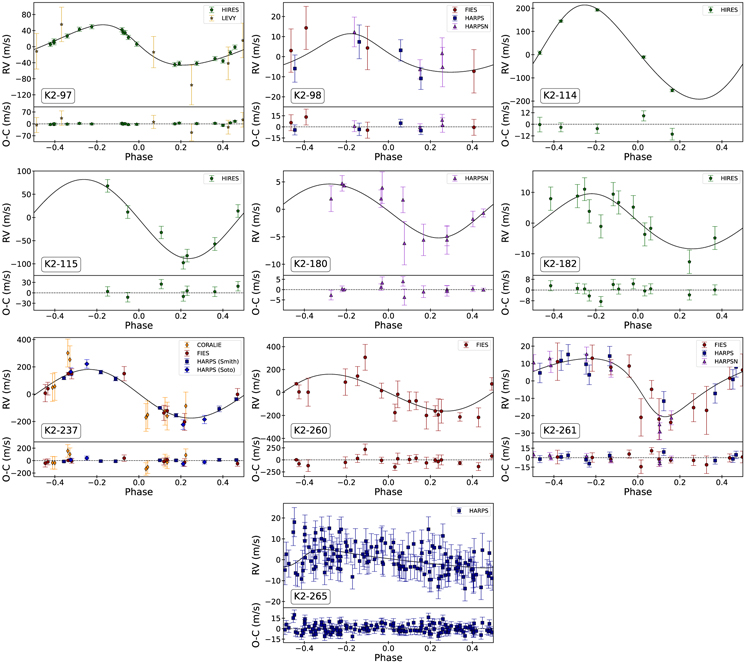
Figure 3. Radial velocities for the 10 systems with archival spectroscopic measurements. The best-fit model from EXOFASTv2 is shown in each panel. Each set of RVs is phased using the best-fit period and Tc determined in the fit, and the residuals are shown below each data set. The references for each set of RVs are listed in Table 1.
Download figure:
Standard image High-resolution imageWe assumed that the RV extraction and metallicity determination was done correctly in the discovery data. An RV jitter term is fit within the EXOFASTv2 analysis to ensure that the uncertainties are properly estimated. In the cases of five or fewer RVs, we placed conservative uniform bounds on the variance of the jitter. The jitter variance for K2-114 and for the Soto et al. (2018) RVs for K2-237 was bounded to ±300 m s−1, and for K2-98 the variance bounds were ±100 m s−1 for the FIES RVs and ±4 m s−1 for HARPS and HARPS-N. For the HARPS RVs of K2-265, we removed three clear outliers that were included in the discovery paper based on visual inspection. 15
3. EXOFASTv2 Global Fits
To analyze the wealth of data for these 26 known K2 exoplanet systems, we used EXOFASTv2 (Eastman et al. 2013, 2019; Eastman 2017) to perform global fits for our sample. EXOFASTv2 is an exoplanet fitting software package that uses Markov Chain Monte Carlo (MCMC) sampling to simultaneously fit parameters for both the planets and the host star. The K2 and TESS photometric observations (Figures 4 and 5), along with any archival RVs (Figure 3), were jointly analyzed to obtain best-fit parameters for planets and host stars.
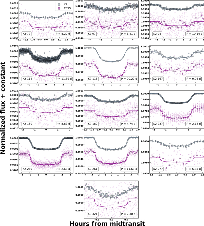
Figure 4. K2 (gray) and TESS (purple) transits for all systems where TESS added significant value to the ephemeris projection. The phase-folded light curves include all data available across the K2 campaigns and TESS sectors for each system and have the best-fit model from EXOFASTv2 overlaid (see Eastman et al. 2013; Eastman 2017; Eastman et al. 2019, for how this is calculated). The system K2 identifier and orbital period of the planet are displayed in each panel. The TESS light curves are shown binned to 12 minutes, and the K2 light curves are unbinned. The discreteness of the K2-237 TESS light curve is likely due to the period being an integer multiple of the exposure time.
Download figure:
Standard image High-resolution image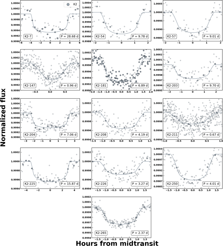
Figure 5. K2 transits for systems that were not recoverable in TESS light curves. The darker points are binned to 30 minutes, and the EXOFASTv2 best-fit model is shown.
Download figure:
Standard image High-resolution image3.1. Stellar Parameters
To characterize the host stars within each fit, we placed a uniform prior from 0 to an upper bound on line-of-sight extinction (Av ) from Schlegel et al. (1998) and Schlafly & Finkbeiner (2011) and Gaussian priors on metallicity ([Fe/H]) and parallax (using Gaia EDR3 and accounting for the small systematic offset reported; Gaia Collaboration et al. 2016, 2021; Lindegren et al. 2021). For consistency, we used metallicity priors for most of the systems from spectra obtained using the Tillinghast Reflector Echelle Spectrograph (TRES; Fűrész 2008) on the 1.5 m Tillinghast Reflector at the Fred L. Whipple Observatory (FLWO). We also included the spectral energy distribution (SED) photometry as reported by Gaia DR2 (Gaia Collaboration et al. 2018), the Wide-field Infrared Survey Explorer (WISE; Cutri et al. 2012), and the Two Micron All Sky Survey (2MASS; Cutri et al. 2003). These values are collated in Table 2, and all priors are listed in the Appendix. We excluded the WISE4 SED values for three systems that had this photometric measurement (K2-115, K2-225, and K2-237) owing to the large uncertainties and because there was a ≳2σ discrepancy with the stellar model. Two other systems (K2-167 and K2-277) had WISE4 measurements that we used in the fits; these are consistent with the stellar models but still have relatively large uncertainties. Within the EXOFASTv2 global fit, the MESA Isochrones and Stellar Tracks (MIST) stellar evolution models (Paxton et al. 2011, 2013, 2015; Choi et al. 2016; Dotter 2016) are used as the base isochrone to better constrain the host star's parameters.
Table 2. Literature Values
| αJ2016 | R.A. | 11:08:22.4996 | 22:32:12.9990 | 22:50:46.0386 | 03:40:54.8458 | 08:31:03.0808 | 08:25:57.1702 | 08:31:31.8984 | 08:26:12.8406 | |
| δJ2016 | decl. | −01:03:57.0898 | −17:32:38.6338 | −14:04:12.0152 | +12:34:20.7938 | +10:50:51.2025 | +11:30:39.9313 | +11:55:20.1168 | +12:16:54.6527 | |
| G | Gaia DR2 G mag | 13.057 ± 0.020 | ⋯ | 14.104 ± 0.020 | 11.920 ± 0.020 | 12.306 ± 0.020 | 12.040 ± 0.020 | 14.275 ± 0.020 | 13.200 ± 0.020 | |
| GBp | Gaia DR2 BP mag | 13.404 ± 0.020 | ⋯ | 14.781 ± 0.020 | 12.485 ± 0.020 | 12.895 ± 0.020 | 12.314 ± 0.020 | 14.806 ± 0.020 | 13.556 ± 0.020 | |
| GRp | Gaia DR2 RP mag | 12.552 ± 0.020 | ⋯ | 13.326 ± 0.020 | 11.236 ± 0.020 | 11.601 ± 0.020 | 11.616 ± 0.020 | 13.615 ± 0.020 | 12.689 ± 0.020 | |
| T | TESS mag | 12.612 ± 0.008 | ⋯ | 13.383 ± 0.006 | 11.287 ± 0.006 | 11.652 ± 0.007 | 11.672 ± 0.008 | 13.667 ± 0.008 | 12.746 ± 0.006 | |
| J | 2MASS J mag | 11.952 ± 0.022 | ⋯ | 12.350 ± 0.024 | 10.384 ± 0.020 | 10.694 ± 0.023 | 11.124 ± 0.022 | 12.835 ± 0.020 | 12.108 ± 0.021 | |
| H | 2MASS H mag | 11.628 ± 0.023 | ⋯ | 11.761 ± 0.022 | 9.910 ± 0.023 | 10.177 ± 0.023 | 10.905 ± 0.025 | 12.386 ± 0.030 | 11.760 ± 0.022 | |
| KS | 2MASS KS mag | 11.564 ± 0.021 | ⋯ | 11.645 ± 0.023 | 9.799 ± 0.020 | 10.035 ± 0.021 | 10.869 ± 0.028 | 12.304 ± 0.030 | 11.724 ± 0.020 | |
| WISE1 | WISE1 mag | 11.527 ± 0.030 | ⋯ | 11.586 ± 0.030 | 9.733 ± 0.030 | 9.990 ± 0.030 | 10.823 ± 0.030 | 12.230 ± 0.030 | 11.658 ± 0.030 | |
| WISE2 | WISE2 mag | 11.572 ± 0.030 | ⋯ | 11.639 ± 0.030 | 9.790 ± 0.030 | 10.090 ± 0.030 | 10.856 ± 0.030 | 12.326 ± 0.030 | 11.700 ± 0.030 | |
| WISE3 | WISE3 mag | 11.554 ± 0.233 | ⋯ | 11.506 ± 0.217 | 9.773 ± 0.054 | 10.026 ± 0.088 | 10.678 ± 0.108 | ⋯ | 11.723 ± 0.249 | |
| WISE4 | WISE4 mag | ⋯ | ⋯ | ⋯ | ⋯ | ⋯ | ⋯ | ⋯ | ⋯ | |
| μα | Gaia p.m. in R.A. | −4.657 ± 0.016 | −5.018 ± 0.021 | 24.311 ± 0.022 | 22.425 ± 0.025 | −1.239 ± 0.018 | −16.165 ± 0.014 | −13.062 ± 0.022 | 15.557 ± 0.018 | |
| μδ | Gaia p.m. in decl. | −23.647 ± 0.012 | −9.804 ± 0.018 | −25.298 ± 0.019 | −37.908 ± 0.015 | −6.694 ± 0.013 | −9.401 ± 0.010 | −2.472 ± 0.016 | −21.630 ± 0.012 | |
| π | Gaia parallax (mas) | 1.451 ± 0.028 | 5.782 ± 0.033 | 3.818 ± 0.029 | 7.111 ± 0.043 | 1.241 ± 0.063 | 1.950 ± 0.042 | 2.130 ± 0.036 | 2.497 ± 0.025 | |
| Param. | K2-147 | K2-167 | K2-180 | K2-181 | K2-182 | K2-203 | K2-204 | K2-208 | K2-211 | |
| αJ2016 | 19:35:19.9267 | 22:26:18.2722 | 08:25:51.4492 | 08:30:12.9870 | 08:40:43.2088 | 00:51:05.6854 | 01:09:31.8015 | 01:23:06.9545 | 01:24:25.4797 | |
| δJ2016 | −28:29:54.5839 | −18:00:42.0516 | +10:14:47.6330 | +10:54:36.5034 | +10:58:58.6242 | −01:11:45.1837 | −00:31:03.9292 | +00:53:20.4074 | +01:42:17.6712 | |
| G | ⋯ | 8.104 ± 0.020 | 12.404 ± 0.020 | 12.562 ± 0.020 | 11.720 ± 0.020 | 12.122 ± 0.020 | 12.889 ± 0.020 | 12.314 ± 0.020 | 12.933 ± 0.020 | |
| GBp | ⋯ | 8.402 ± 0.020 | 12.817 ± 0.020 | 12.945 ± 0.020 | 12.190 ± 0.020 | 12.614 ± 0.020 | 13.223 ± 0.020 | 12.702 ± 0.020 | 13.399 ± 0.020 | |
| GRp | ⋯ | 7.689 ± 0.020 | 11.839 ± 0.020 | 12.036 ± 0.020 | 11.122 ± 0.020 | 11.493 ± 0.020 | 12.408 ± 0.020 | 11.781 ± 0.020 | 12.333 ± 0.020 | |
| T | ⋯ | 7.728 ± 0.006 | 11.896 ± 0.006 | 12.087 ± 0.006 | 11.170 ± 0.006 | 11.547 ± 0.006 | 12.461 ± 0.006 | 11.833 ± 0.006 | 12.383 ± 0.007 | |
| J | ⋯ | 7.202 ± 0.021 | 11.146 ± 0.023 | 11.438 ± 0.022 | 10.408 ± 0.021 | 10.773 ± 0.024 | 11.839 ± 0.021 | 11.164 ± 0.026 | 11.624 ± 0.024 | |
| H | ⋯ | 6.974 ± 0.038 | 10.747 ± 0.026 | 11.082 ± 0.021 | 9.994 ± 0.022 | 10.281 ± 0.026 | 11.569 ± 0.026 | 10.824 ± 0.022 | 11.205 ± 0.022 | |
| KS | ⋯ | 6.887 ± 0.034 | 10.677 ± 0.026 | 11.026 ± 0.021 | 9.913 ± 0.023 | 10.206 ± 0.023 | 11.478 ± 0.021 | 10.746 ± 0.020 | 11.104 ± 0.024 | |
| WISE1 | ⋯ | 6.810 ± 0.055 | 10.619 ± 0.030 | 10.999 ± 0.030 | 9.845 ± 0.030 | 10.145 ± 0.030 | 11.468 ± 0.030 | 10.697 ± 0.030 | 11.074 ± 0.030 | |
| WISE2 | ⋯ | 6.866 ± 0.030 | 10.667 ± 0.030 | 11.062 ± 0.030 | 9.917 ± 0.030 | 10.217 ± 0.030 | 11.507 ± 0.030 | 10.739 ± 0.030 | 11.128 ± 0.030 | |
| WISE3 | ⋯ | 6.906 ± 0.030 | 10.599 ± 0.099 | 11.041 ± 0.205 | 9.896 ± 0.054 | 10.100 ± 0.083 | 11.279 ± 0.173 | 10.645 ± 0.089 | 10.933 ± 0.093 | |
| WISE4 | ⋯ | 6.917 ± 0.100 | ⋯ | ⋯ | ⋯ | ⋯ | ⋯ | ⋯ | ⋯ | |
| μα | −31.399 ± 0.016 | 73.590 ± 0.028 | 97.243 ± 0.013 | 16.936 ± 0.014 | −65.130 ± 0.029 | −11.103 ± 0.021 | −3.598 ± 0.026 | −26.433 ± 0.019 | 48.694 ± 0.022 | |
| μδ | −147.502 ± 0.015 | −114.502 ± 0.024 | −89.214 ± 0.010 | −33.182 ± 0.012 | 1.544 ± 0.022 | 0.450 ± 0.020 | −30.522 ± 0.018 | −39.656 ± 0.014 | −10.262 ± 0.017 | |
| π | 11.027 ± 0.033 | 12.457 ± 0.071 | 4.936 ± 0.041 | 2.805 ± 0.040 | 6.510 ± 0.052 | 5.937 ± 0.056 | 1.840 ± 0.052 | 3.859 ± 0.048 | 3.604 ± 0.055 | |
| Param. | K2-225 | K2-226 | K2-237 | K2-250 | K2-260 | K2-261 | K2-265 | K2-277 | K2-321 | References |
| αJ2016 | 12:26:09.8617 | 12:14:34.9587 | 16:55:04.5232 | 12:20:07.5686 | 05:07:28.1596 | 10:52:07.7541 | 22:48:07.5960 | 13:28:03.8821 | 10:25:37.3214 | 1 |
| δJ2016 | −09:37:29.3675 | −09:33:45.4617 | −28:42:38.1039 | −08:58:32.6688 | +16:52:03.6985 | +00:29:35.3793 | −14:29:41.2159 | −15:56:16.7278 | +02:30:49.9241 | 1 |
| G | 11.520 ± 0.020 | 12.092 ± 0.020 | 11.467 ± 0.020 | 13.973 ± 0.020 | 12.467 ± 0.020 | 10.459 ± 0.020 | 10.928 ± 0.020 | 10.121 ± 0.020 | ⋯ | 2 |
| GBp | 11.929 ± 0.020 | 12.545 ± 0.020 | 11.776 ± 0.020 | 14.484 ± 0.020 | 12.798 ± 0.020 | 10.872 ± 0.020 | 11.337 ± 0.020 | 10.495 ± 0.020 | ⋯ | 2 |
| GRp | 10.984 ± 0.020 | 11.492 ± 0.020 | 11.013 ± 0.020 | 13.324 ± 0.020 | 11.974 ± 0.020 | 9.917 ± 0.020 | 10.364 ± 0.020 | 9.624 ± 0.020 | ⋯ | 2 |
| T | 11.028 ± 0.007 | 11.547 ± 0.006 | 11.066 ± 0.006 | 13.379 ± 0.006 | 12.036 ± 0.007 | 9.962 ± 0.007 | 10.422 ± 0.008 | 9.666 ± 0.006 | ⋯ | 3 |
| J | 10.362 ± 0.023 | 10.697 ± 0.023 | 10.508 ± 0.023 | 12.539 ± 0.026 | 11.400 ± 0.023 | 9.337 ± 0.030 | 9.726 ± 0.026 | 9.081 ± 0.034 | ⋯ | 4 |
| H | 10.046 ± 0.021 | 10.307 ± 0.023 | 10.268 ± 0.022 | 12.078 ± 0.022 | 11.189 ± 0.032 | 8.920 ± 0.042 | 9.312 ± 0.022 | 8.748 ± 0.071 | ⋯ | 4 |
| KS | 9.954 ± 0.023 | 10.223 ± 0.023 | 10.217 ± 0.023 | 12.016 ± 0.024 | 11.093 ± 0.021 | 8.890 ± 0.022 | 9.259 ± 0.027 | 8.687 ± 0.024 | ⋯ | 4 |
| WISE1 | 9.915 ± 0.030 | 10.166 ± 0.030 | 10.105 ± 0.030 | 11.878 ± 0.030 | 11.039 ± 0.030 | 8.828 ± 0.030 | 9.178 ± 0.030 | 8.630 ± 0.030 | ⋯ | 5 |
| WISE2 | 9.978 ± 0.030 | 10.204 ± 0.030 | 10.129 ± 0.030 | 11.971 ± 0.030 | 11.036 ± 0.030 | 8.897 ± 0.030 | 9.213 ± 0.030 | 8.675 ± 0.030 | ⋯ | 5 |
| WISE3 | 9.932 ± 0.057 | 10.118 ± 0.083 | 9.972 ± 0.077 | 11.534 ± 0.259 | 10.895 ± 0.129 | 8.819 ± 0.031 | 9.162 ± 0.040 | 8.649 ± 0.030 | ⋯ | 5 |
| WISE4 | ⋯ | ⋯ | ⋯ | ⋯ | ⋯ | ⋯ | ⋯ | 8.418 ± 0.261 | ⋯ | 5 |
| μα | −38.138 ± 0.023 | −22.324 ± 0.023 | −8.568 ± 0.035 | −50.359 ± 0.030 | 0.646 ± 0.018 | −23.709 ± 0.020 | 30.138 ± 0.020 | −98.828 ± 0.024 | 50.920 ± 0.025 | 1 |
| μδ | −8.190 ± 0.017 | 2.109 ± 0.021 | −5.625 ± 0.022 | 9.874 ± 0.018 | −6.034 ± 0.013 | −43.888 ± 0.017 | −23.359 ± 0.016 | −35.889 ± 0.016 | −109.167 ± 0.022 | 1 |
| π | 2.796 ± 0.045 | 4.807 ± 0.074 | 3.298 ± 0.071 | 2.476 ± 0.036 | 1.498 ± 0.043 | 4.685 ± 0.043 | 7.189 ± 0.051 | 8.842 ± 0.062 | 13.009 ± 0.053 | 1 |
Note. The uncertainties of the photometry have a systematic error floor applied. The SEDs were not used for K2-54, K2-147, and K2-321 (see Section 3). Proper motions are taken from the Gaia EDR3 archive and are in J2016. Parallaxes from Gaia EDR3 have a correction applied according to Lindegren et al. (2021). Parallax for K2-277 is from Gaia DR2 and has been corrected according to Lindegren et al. (2018).
References. (1) Gaia Collaboration et al. 2021; (2) Gaia Collaboration et al. 2018; (3) Stassun et al. 2018; (4) Cutri et al. 2003; (5) Cutri et al. 2012.
3.2. Low-mass Stars
Stellar evolutionary models struggle to constrain low-mass stars (≲0.6 M⊙; Mann et al. 2015) and are thus unreliable. For the three systems that fell into this category (K2-54, K2-147, and K2-321), we used the equations from Mann et al. (2015, 2019) that relate the apparent magnitude in the KS
band ( ) to M* and R* to set a starting point with wide 5% Gaussian priors for these parameters. We excluded the SEDs from these fits and did not use the MIST models, fitting only the light curves (these systems did not have RV measurements). For this reason, we caution that the stellar parameters for these systems are unreliable. We also did not use the limb-darkening tables from Claret (2017) for the low-mass stars, as is the default in EXOFASTv2 for fitting the u1 and u2 coefficients, but rather placed starting points based on tables from Claret & Bloemen (2011; Eastman et al. 2013) with a conservative Gaussian prior of 0.2 (Patel & Espinoza 2022).
3.3. Contamination
For systems with TESS contamination ratios specified in the TESS input catalog (TICv8; Stassun et al. 2018) and a clear transit detected in both K2 and TESS, we fit for a dilution term 16 on the TESS photometry with a 10% Gaussian prior. This accounts for any nearby sources that may contribute flux to the target aperture that were unknown at the time the TESS Input Catalog was created. Although the TESS PDCSAP light curves are corrected for contamination, fitting the dilution allows an independent check on the contamination ratio correction performed by the SPOC pipeline. Fitting a dilution term for only the TESS photometry assumes that the K2 aperture has been correctly decontaminated or is comparatively uncontaminated, which is based on K2 having a significantly smaller pixel scale than TESS (4'' and 21'' for K2 and TESS, respectively). However, it is possible that there is still a level of contamination within the K2 aperture that might be identified through high-resolution imaging. We checked the K2 aperture for all of our targets to identify any major sources of contamination from the Gaia EDR3 catalog. We define contaminants as having flux ratios with the target star that are much larger than the uncertainties of the transit depth. To correct for the contaminating light, we followed the method from Rampalli et al. (2019) to account for the fraction of the flux within the aperture that belonged to our targets (Fstar) as opposed to the contaminating stars based on the Gaia G-band fluxes. We found significant contamination for K2-54 (Fstar ≈ 0.56) and K2-237 (Fstar ≈ 0.98; the latter was originally discussed in Ikwut-Ukwa et al. 2020). Several other systems had potential faint contaminants; however, the global fit for the system with the next highest level of contamination (K2-250; Fstar ≈ 0.98) did not change within uncertainties before and after flux correction, so we did not apply corrections to any systems other than K2-54 and K2-237.
3.4. Global Fits
We ran a short preliminary fit for each system to identify any potential issues, e.g., particularly shallow transits, and then ran a final fit to convergence. For a fit to be accepted as converged, we adopted the default EXOFASTv2 criteria of TZ > 1000, where TZ is the number of independent draws, and a slightly loose Gelman–Rubin value of <1.02 due to some transits being very shallow in TESS, resulting in long runtimes for the global fits. Within EXOFASTv2, we opted to reject all flat and negative transit models, which ensured a more reliable recovery of marginal transits (Eastman et al. 2019). We did not fit for transit timing variations (TTVs), but we plan to explore this in future papers.
Shallow transits clearly detected in K2 were not always evident in the TESS light curves, as the latter are necessarily noisier owing to the smaller collecting area of the telescope (see Section 4.6 for discussion). For these systems we ran a K2-only fit to convergence and a short preliminary fit (Gelman–Rubin value of ∼1.1, Tz ∼ 100). To assess whether it was advantageous to include the TESS light curves, we required that certain criteria be met before running the K2 and TESS fit to convergence. First, we compared the improvement on uncertainties for parameters such as period and TC and projected these to the year 2030. If the uncertainties were notably smaller when including TESS data, we continued by visually inspecting the transits modeled by EXOFASTv2. For extremely marginal transits, we further binned the phased light curves to determine whether the transit was indeed visible. If the transit in TESS was still not obvious, we inspected the probability distribution functions (pdf's) output by EXOFASTv2 for clearly non-Gaussian distributions for key parameters, particularly period. If the period was not well constrained (e.g., multimodal) even with the increased baseline of TESS, we excluded the TESS light curve from the fit. A multimodal period indicates that the MCMC identified different transit solutions based on the TESS data, implying that the TESS transits are not securely enough detected to update the ephemeris.
We ultimately excluded any TESS light curves where the transit has S/N ≲ 7. As these are all previously confirmed planets, we adopted a less conservative S/N for bona fide transits in TESS compared to what is required for initial planet verification. This S/N threshold was chosen because the first system below this cut (K2-265, S/N = 6.0) had a multimodal posterior for period, and all other systems with lower S/N exhibited similar issues. Conversely, the system just above this threshold (K2-277, S/N = 8.1) has a broad but Gaussian period posterior, with no other systems above this S/N having unreliable pdf's.
Using this threshold, 13 of the 26 systems did not have recoverable TESS transits, so these were globally fit using only their K2 light curves (Figure 5). While these systems will not have as significant improvement on their ephemerides, we still provide the updated parameters to include them in our final catalog of self-consistent parameters.
4. Results and Discussion
We updated the system parameters for 26 single-planet systems discovered by K2 and reobserved by TESS, four of which were part of the pilot study for the K2 and TESS Synergy (K2-114, K2-167, K2-237, and K2-261; Ikwut-Ukwa et al. 2020). The values from the EXOFASTv2 global fits are shown in the Appendix. Here we address any points of interest for individual systems and for the sample as a whole.
4.1. Ephemeris Improvement
As addressed in Section 1, a major incentive for refitting all K2 and TESS systems is to update their ephemerides to provide the community with accurate transit times for observing with existing and upcoming facilities. Figures 6 and 7 show the projected transit timing uncertainties for our sample extrapolated to 2035, with markers indicating the expected launches for ongoing and future missions. The uncertainties on the transit times are calculated by standard error propagation,

where  is the uncertainty on future transit time,
  is the uncertainty on the fitted optimal time of conjunction, ntrans is the number of transits that occurred between time stamps, and σP
is uncertainty on the period. For the future transit times using the results of the EXOFASTv2 global fits, we used the optimal time of conjunction in order to minimize the covariance between TC
and P. However, T0 is not generally available for the K2 discovery parameters, so for the projected uncertainties on transit times for the original K2 values we used TC
.
is the uncertainty on the fitted optimal time of conjunction, ntrans is the number of transits that occurred between time stamps, and σP
is uncertainty on the period. For the future transit times using the results of the EXOFASTv2 global fits, we used the optimal time of conjunction in order to minimize the covariance between TC
and P. However, T0 is not generally available for the K2 discovery parameters, so for the projected uncertainties on transit times for the original K2 values we used TC
.

Figure 6. Projected uncertainties for transit times ( ) for systems with transits detected in both K2 and TESS. The shaded regions represent the 1σ, 2σ, and 3σ uncertainties, where gray is the uncertainty from the K2 ephemerides listed in Table 1 and purple is our updated version using EXOFASTv2. The vertical dashed lines show the expected or actual launch years for missions for which these systems would be prospective targets (JWST: red; NGRST: orange; ARIEL: yellow). Note that the y-axis scale is different in each panel.
Download figure:
Standard image High-resolution image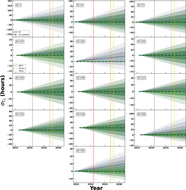
Figure 7. Same as Figure 6, but for systems with transits only detectable in the K2 light curves. The shaded regions represent the 1σ, 2σ, and 3σ uncertainties, where gray is the uncertainty from the K2 ephemerides listed in Table 1 and green is our updated version using EXOFASTv2. The vertical dashed lines show the expected or actual launch years for missions for which these systems would be prospective targets (JWST: red; NGRST: orange; ARIEL: yellow). The ephemeris for K2-181 is significantly improved owing to the inclusion of data from K2 Campaign 18.
Download figure:
Standard image High-resolution imageAs expected, systems for which we excluded the TESS data owing to shallow transits were not improved on the same scale as those with significant TESS transits. For the K2 and TESS systems, the updated global fits were able to reduce most uncertainties from hours to minutes within the scope of some of the major facilities in the near future (Figure 6). For the 13 systems with detected TESS transits, the average 3σ uncertainty on the future transit time by the year 2030 was reduced from 26.7 to 0.35 hr (Table 3).
Table 3. Ephemerides as of Discovery Compared to Our Updated Values for Systems with K2 and TESS Transits, with the 3σ Uncertainty on Future Transit Time by the Year 2030
| P (days) | Tc (BJD) | 3σ2030 | TSM | |
|---|---|---|---|---|
| K2-77 | ||||
| Discovery |

|
| 17.4 hr | |
| Updated |
|
| 22 minutes | 0.18 |
| K2-97 | ||||
| Discovery |

|
| 84.8 hr | |
| Updated | 8.407115 ± 0.000023 |
| 58 minutes | ⋯ |
| K2-98 | ||||
| Discovery | 10.13675 ± 0.00033 | 2457145.9807 ± 0.0012 | 12.6 hr | |
| Updated |
|
| 19 minutes | 0.09 |
| K2-114 | ||||
| Discovery |

| 2457174.49729 ± 0.00033 | 5.9 hr | |
| Updated |
| 2457687.08869 ± 0.00016 | 6 minutes | ⋯ |
| K2-115 | ||||
| Discovery |
| 2457157.15701 ± 0.00025 | 42 minutes | |
| Updated | 20.2729914 ± 0.0000050 | 2457522.07014 ± 0.00017 | 5 minutes | ⋯ |
| K2-167 | ||||
| Discovery |

|
| 40.8 hr | |
| Updated |

|

| 48 minutes | 0.30 |
| K2-180 | ||||
| Discovery | 8.8665 ± 0.0003 | 2457143.390 ± 0.002 | 13.0 hr | |
| Updated |

|
| 26 minutes | 0.10 |
| K2-182 | ||||
| Discovery | 4.7369683 ± 0.0000023 | 2457719.11517 ± 0.00028 | 10 minutes | |
| Updated | 4.7369696 ± 0.0000017 |
| 8 minutes | 0.10 |
| K2-237 | ||||
| Discovery | 2.18056 ± 0.00002 | 2457684.8101 ± 0.0001 | 3.2 hr | |
| Updated | 2.18053332 ± 0.00000054 |
| 5 minutes | ⋯ |
| K2-260 | ||||
| Discovery | 2.6266657 ± 0.0000018 | 2457820.738135 ± 0.00009 | 14 minutes | |
| Updated | 2.62669762 ± 0.00000066 |
| 5 minutes | ⋯ |
| K2-261 | ||||
| Discovery | 11.63344 ± 0.00012 |
| 3.4 hr | |
| Updated | 11.6334681 ± 0.0000044 |

| 7 minutes | 0.55 |
| K2-277 | ||||
| Discovery |

|
| 21.5 hr | |
| Updated |

| 2457303.4771 ± 0.0010 | 48 minutes | 0.23 |
| K2-321 | ||||
| Discovery | 2.298 ± 0.001 | 2457909.17 | 144.0 hr | |
| Updated |

|
| 15 minutes | ⋯ |
Note. The discovery values are taken from the K2 references listed in Table 1. The TC for the updated values is T0 as determined by our global fits. The TSM value is normalized to the K2 catalog (see Section 4.2).
Download table as: ASCIITypeset image
Systems for which we only included the K2 light curves had significantly less improvement on the precision of predicted transit times. However, the ephemeris for K2-181 was considerably refined owing to the addition of data from K2 Campaign 18, which was not included in any previous analysis of this system. Excluding K2-181, there was a slight reduction of the average 3σ uncertainty from 43.2 to 35.6 hr (Table 4). The small improvement for some systems is likely due to using optimized K2 light curves obtained from the pipeline described in Section 2.1, in conjunction with our fits including both the planet and the host star.
Table 4. Ephemerides as of Discovery Compared to Our Updated Values for Systems with Only K2 Transits, with the 3σ Uncertainty on Future Transit Time by the Year 2030
| P (days) | Tc (BJD) | 3σ2030 | TSM | |
|---|---|---|---|---|
| K2-7 | ||||
| Discovery | 28.67992 ± 0.00947 | 2456824.6155 ± 0.0149 | 135.0 hr | |
| Updated |

|
| 68.8 hr | 0.04 |
| K2-54 | ||||
| Discovery | 9.7843 ± 0.0014 | 2456982.9360 ± 0.0053 | 56.8 hr | |
| Updated |

| 2457002.5042 ± 0.0029 | 50.6 hr | ⋯ |
| K2-57 | ||||
| Discovery | 9.0063 ± 0.0013 | 2456984.3360 ± 0.0048 | 57.3 hr | |
| Updated |

| 2457011.3568 ± 0.0023 | 50.4 hr | 0.07 |
| K2-147 | ||||
| Discovery | 0.961918 ± 0.000013 |

| 5.0 hr | |
| Updated | 0.961939 ± 0.000029 |
| 11.2 hr | ⋯ |
| K2-181 | ||||
| Discovery |

|
| 23.9 hr | |
| Updated | 6.893813 ± 0.000011 | 2457778.0262 ± 0.0012 | 0.5 hr | 0.09 |
| K2-203 | ||||
| Discovery |

|
| 49.7 hr | |
| Updated | 9.6952 ± 0.0014 |
| 52.7 hr | 0.01 |
| K2-204 | ||||
| Discovery |

|
| 33.6 hr | |
| Updated |

| 2457431.7872 ± 0.0022 | 33.6 hr | 0.07 |
| K2-208 | ||||
| Discovery |

|
| 21.0 hr | |
| Updated | 4.19097 ± 0.00023 | 2457430.0390 ± 0.0016 | 20.0 hr | 0.08 |
| K2-211 | ||||
| Discovery | 0.669532 ± 0.000019 | 2457395.82322 ± 0.00160 | 10.4 hr | |
| Updated |

| 2457432.6479 ± 0.0013 | 17.2 hr | 0.01 |
| K2-225 | ||||
| Discovery |

|
| 42.2 hr | |
| Updated |

|
| 44.3 hr | 0.07 |
| K2-226 | ||||
| Discovery |

|
| 39.8 hr | |
| Updated |

| 2457620.0082 ± 0.0020 | 40.3 hr | 0.09 |
| K2-250 | ||||
| Discovery |

|
| 52.5 hr | |
| Updated | 4.01392 ± 0.00029 | 2457620.2535 ± 0.0015 | 25.4 hr | 0.09 |
| K2-265 | ||||
| Discovery | 2.369172 ± 0.000089 | 2456981.6431 ± 0.0016 | 14.9 hr | |
| Updated |

|
| 9.8 hr | 0.10 |
Note. The discovery values are taken from the K2 references listed in Table 1. The TC for the updated values is T0 as determined by our global fits. The TSM value is normalized to the K2 catalog (see Section 4.2).
Download table as: ASCIITypeset image
For systems with RV measurements, our ephemeris comparison uses uncertainties taken from previous analyses that included the RVs along with the K2 data. The uncertainties for systems without RVs are taken from the most recent study that included light curves from K2. There are a handful of exceptions to this rule: for K2-77 we use the values from Mayo et al. (2018), as Gaidos et al. (2017) only have three RV measurements, which is insufficient for our EXOFASTv2 fits; for K2-97, we use the values from Livingston et al. (2018a), as no Tc was presented in the analysis by Grunblatt et al. (2018) that included RVs; for K2-237 we use the less precise values from Soto et al. (2018), which are consistent with our results, rather than those from Smith et al. (2019), which have a ∼4σ discrepancy with our findings (this was also found in the pilot study; Ikwut-Ukwa et al. 2020).
As mentioned in Section 3.4, half of our sample did not have transits deep enough to be recovered by TESS. This presents a challenge for updating the transit times for these systems. If these systems are observed in future TESS sectors, it is possible that the S/N will increase sufficiently to include in a global fit. We will continue to monitor these and will include them in future releases, if this is the case.
4.1.1. K2-167
We note the use of an errant stellar metallicity prior used in the pilot study, where 0.45 instead of −0.45 (as reported by Mayo et al. 2018) was used as the Gaussian center. While this may have affected the solutions of stellar and planetary parameters, it would not have significantly altered the ephemeris.
4.1.2. K2-260
There is a clear discrepancy between the previously published ephemeris and our updated version (see Figure 6), well beyond a 3σ level. To test whether this was an artifact of our global fit, we ran a fit using only the K2 light curves and compared the results to the original and K2 and TESS fits. Our K2-only fit was consistent with our K2 and TESS ephemeris and still in disagreement with the original results, suggesting that our updated fit provides the optimal ephemeris. It is possible that the original light curves introduced systematics in the discovery analysis, or the inclusion of additional follow-up data affected the ephemeris, but this is not clear. In any case, the consistency between our K2-only and K2 and TESS ephemerides (and no other system showing similar issues) gives us confidence in our results.
4.1.3. K2-261
As discussed in the pilot study (Ikwut-Ukwa et al. 2020), the pdf's for some stellar parameters (particularly age and mass) of K2-261 exhibit distinct bimodality that is likely due to the star being at a main-sequence transition point (and not associated with the poor fits of shallow transits discussed in Section 3.4), causing difficulties with fitting the MIST isochrones to the data to constrain age. We followed the same procedure from Ikwut-Ukwa et al. (2020), splitting the posterior at the minimum probability for M* between the two Gaussian peaks (at M* = 1.19 M⊙; see Figure 5 of Ikwut-Ukwa et al. 2020) and extracting two separate solutions for each peak. The low- and high-mass solutions have probabilities of 59.9% and 40.1%, respectively. We list both solutions in Table 9; however, we use the low-mass solution for all figures, as this has the higher probability. The different stellar mass solutions do not affect the ephemeris projection for this planet.
4.1.4. Comparison to Pilot Study
The ephemerides were slightly improved for the four systems from the pilot study, the most significant being K2-167 (from 1.1 hr to 48 minutes) and K2-261 (from 30 minutes to 7 minutes). We did not expect to see major improvement because the baseline of new TESS sectors is relatively short compared to that of K2 and the TESS primary mission.
4.2. TSM
We calculated the transmission spectroscopy metric (TSM; Kempton et al. 2018) normalized to the entire K2 catalog for the planets in this sample to gauge the value of atmospheric follow-up (Tables 3 and 4; Figure 8). As the TSM is dependent on stellar parameters, we excluded the three systems for which we did not fit the host star (K2-54, K2-147, K2-321; see Section 3). The TSM is only valid for planets with Rp < 10 R⊕, which removes a further five planets from this calculation (K2-97, K2-114, K2-115, K2-237, and K2-260). We used the parameters from the global fits for the systems in this paper for the TSM calculation, and for all other systems we retrieved the necessary parameters from the default parameter sets within the NEA, only including systems for which the parameters were either measured or able to be derived from other parameters (i.e. Mp and Teq). The system with the highest raw TSM value (K2-141c, TSM=1068.7) was removed before normalization as it was a factor of ~8 times larger than the next highest TSM and thus significantly skewed the rest of the sample. Future work in this project to update ephemerides will prioritize planets with high TSMs relative to the entire K2 catalog.
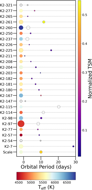
Figure 8. Architecture for each system showing the values from the global fits for the 26 systems in this analysis. The host stars are the leftmost circles, with their temperatures indicated by color and relative radius shown by size. The rightmost circles represent the planets, with size showing relative radius and color indicating their TSM normalized to the K2 catalog. The radii of the star and planet within each system are not scaled to each other. Systems for which we did not fit stellar parameters and planets that do not have a calculated TSM are represented by open circles (see Section 4.2). An example ofa Sun-like star hosting a Jupiter-like planet with a 10-day period and scaled TSM of 0.5 is shown for reference.
Download figure:
Standard image High-resolution image4.3. The Sample
While the systems in this analysis span a broad range of stellar temperatures and planet masses, most planets have orbital periods ≲10 days and radii ≲5 R⊕ (Figures 8 and 9). Planet masses range from 2.6 to 639 M⊕, and host stars include M dwarfs to F-type spectral classifications. This demonstrates the diversity of the original K2 sample as largely community-selected targets. Figure 9 shows how this sample compares to other known exoplanets.

Figure 9. Radius vs. mass for all confirmed exoplanets (gray; values taken from the NEA) and those in our work (using the median values from the EXOFASTv2 output). The 10 systems with planetary masses measured through RVs are indicated by diamonds, while the planets without RVs that have masses obtained from the Chen & Kipping (2017) mass–radius relations are shown as crosses. The points are colored by the effective temperature of the host star and are open for the three systems without fitted stellar parameters.
Download figure:
Standard image High-resolution image
4.4. Transit Timing Variations
We did not fit for TTVs in this study. We would expect these to manifest as a significant change in ephemeris over time, whereas all of the systems studied here have updated ephemerides consistent to within 3σ of the original K2 ephemeris (except K2-260; see Section 4.1.2). Therefore, any TTVs that may be present are currently too small to detect for these systems. Differences in the ephemerides on the 1σ–3σ level are likely due to the addition of the TESS light curves.
4.5. Candidate Planets
We note that a couple of the systems in our analysis have additional candidate planets (K2-203 and K2-211). However, we ignore these for the purpose of updating ephemerides of known exoplanets that are more likely future targets for missions such as JWST, but we plan to revisit these in a future paper addressing multiplanet systems.
4.6. K2 versus TESS
It is not surprising that relatively shallow K2 transits were not detected by TESS. Kepler and TESS were designed to observe different stellar demographics, resulting in different photometric capabilities. Kepler was built with the intent to explore the number of near-Earth-sized planets close to their respective habitable zones around distant stars with apparent magnitudes ≲16. The original Kepler mission could reach a precision of ∼20 parts per million (ppm), which was generally the same for the K2 mission (Vanderburg & Johnson 2014; Vanderburg et al. 2016).
On the other hand, TESS is focused on nearby, brighter stars with magnitude ≲12. The precision of TESS has a floor at ∼20 ppm at 1 hr for the brightest stars with Tmag < 4, but it is more realistically ≳100 ppm for the majority of stars. Due to the all-sky nature of the TESS missions, observing sectors last on average 27 days for efficient sky coverage. K2 campaigns were around 80 days in duration, meaning that the same targets may have ∼3 times as many transits observed by K2.
While TESS may not be able to recover all K2 systems, the ones it can detect will have vastly improved ephemerides as demonstrated in Figure 6. Our analysis indicates that TESS transits with S/N ≳ 7 are recoverable, and while this places a limit on the scope of this reanalysis, we can potentially gain access for reobservation of at least half of known K2 planets. It is possible that future TESS missions that reobserve the planets with currently marginal transits (S/N ∼ 5–6) will increase the S/N enough for a significant detection. However, for transits with S/N ≲ 5, it is unlikely that more TESS observations will result in recoverable transits.
4.7. Future Work
With several major facilities able to characterize exoplanets in extensive detail planned to come online within the next decade, not having accurate and precise transit times is a relevant issue. The K2 and TESS Synergy aims to solve the problem of degrading ephemerides for all K2 systems reobserved by TESS (with clearly detectable transits as shown by this effort). Assuming that TESS will reobserve all K2 systems throughout its extended missions, we expect to be able to update the ephemerides for around half of K2 planets (∼250 planets) with transits deep enough to be detected by TESS, based on this study. Over the next couple of years, we plan to reanalyze the remaining K2 systems with current TESS overlap, providing the updated parameters to the community. In future batches, we will place a focus on systems that are potentially well suited as JWST targets for atmospheric studies based on their TSMs. While we do not see strong evidence for TTVs in the current work, we will make note of this in future for any systems with significant change in ephemeris, particularly for known multiplanet systems where this would be more readily detectable.
5. Conclusion
Past efforts to create and analyze homogeneous populations of exoplanet parameters have led to great insight into major questions in planetary formation and evolution (Wang et al. 2014; Fulton et al. 2017; Fulton & Petigura 2018). The K2 and TESS Synergy is uniting NASA's planet-hunting missions and focuses on extending the scientific output of both telescopes by creating a self-consistent catalog for the K2 and TESS sample while providing the community with updated ephemerides to efficiently schedule future characterization observations with facilities like JWST (Gardner et al. 2006). As well as refreshing stale ephemerides, this provides a uniform way of addressing any inconsistencies between the original K2 ephemeris and the updated value from TESS. In this paper, we have presented updated parameters for 26 single-planet systems originally discovered by K2 and more recently reobserved by TESS during its primary and extended missions. Following from the success of the pilot study (Ikwut-Ukwa et al. 2020), we have significantly reduced the uncertainties on transit times for the 13 systems with transits detectable in TESS from hours down to minutes through the JWST operations window (∼2030). Assuming that the current sample is representative of the entire K2 catalog, we expect significant improvement on ephemerides for about half of the systems revisited by TESS, with the goal of a ∼250-system catalog of parameters that will be publicly available. As TESS continues to reobserve large portions of the entire sky during its current and possible future extended missions, there will be a well-suited opportunity to conduct this analysis on all known exoplanets, possibly leading to key insights into the evolutionary processes of exoplanets.
We thank the anonymous referee for the constructive feedback that helped improve this manuscript. E.T. and J.E.R. acknowledge support for this project from NASA's TESS Guest Investigator program (G04205, P.I. Rodriguez). We thank Grace Gillig and Kaliab Kebede for their contribution in determining the target list for the K2 & TESS Synergy GI Cycle 4 proposal that was conducted as part of the 2020-2021 Harvard-MIT Science Research Mentoring Program (SRMP). This research has made use of SAO/NASA's Astrophysics Data System Bibliographic Services. This research has made use of the SIMBAD database, operated at CDS, Strasbourg, France. This work has made use of data from the European Space Agency (ESA) mission Gaia (https://www.cosmos.esa.int/gaia), processed by the Gaia Data Processing and Analysis Consortium (DPAC, https://www.cosmos.esa.int/web/gaia/dpac/consortium). Funding for the DPAC has been provided by national institutions, in particular the institutions participating in the Gaia Multilateral Agreement. This work makes use of observations from the LCO network. This research made use of Lightkurve, a Python package for Kepler and TESS data analysis. This research has made use of the NASA Exoplanet Archive, which is operated by the California Institute of Technology, under contract with the National Aeronautics and Space Administration under the Exoplanet Exploration Program.
Funding for the TESS mission is provided by NASA's Science Mission directorate. We acknowledge the use of public TESS Alert data from pipelines at the TESS Science Office and at the TESS Science Processing Operations Center. This research has made use of the Exoplanet Follow-up Observation Program website, which is operated by the California Institute of Technology, under contract with the National Aeronautics and Space Administration under the Exoplanet Exploration Program. Resources supporting this work were provided by the NASA High-End Computing (HEC) Program through the NASA Advanced Supercomputing (NAS) Division at Ames Research Center for the production of the SPOC data products. The data presented in this paper were obtained from the Mikulski Archive for Space Telescopes (MAST) at the Space Telescope Science Institute. The K2 and TESS light curves listed in Table 1 can be accessed at doi:10.17909/r4j7-gg73. TESS data from Sectors 2–46 were used in this analysis.
Facilities: TESS - , K2 - , Keck (HIRES) - , Lick Observatory 2.4 m (Levy) - , Nordic Optical 2.56 m (FIES) - , La Silla 3.6 m (HARPS) - , Telescopio Nazionale Gailieo 3.58 m (HARPS-N) - , La Silla 1.2 m (CORALIE) - , FLWO 1.5 m (Tillinghast Reflector Echelle Spectrograph). -
Software: Lightkurve (Lightkurve Collaboration et al. 1812), EXOFASTv2 (Eastman et al. 2013, 2019).
Appendix: Additional Tables
Tables 5–12 show the output from EXOFASTv2 for all 26 systems. In Tables 5–9, the priors we placed on parallax, metallicity, extinction and dilution are shown (see Sections 3.1 and 3.3 for how these were determined), followed by the median values for stellar and planetary parameters. Tables 10 and 11 show the transit parameters for the K2-only fits and the fits with K2 and TESS transits, respectively. Table 12 contains the RV parameters for the systems with spectroscopic measurements.
Table 5. Median Values and 68% Confidence Intervals
| K2-7 | K2-54' | K2-57 | K2-77 | K2-97 | K2-98 | ||
|---|---|---|---|---|---|---|---|
| Priors: | |||||||
| π | Gaia parallax (mas) |
![${ \mathcal G }[1.45113,0.02810]$](https://content.cld.iop.org/journals/1538-3881/165/4/155/revision1/ajacaf03ieqn63.gif)
| ⋯ |
![${ \mathcal G }[3.81841,0.02910]$](https://content.cld.iop.org/journals/1538-3881/165/4/155/revision1/ajacaf03ieqn64.gif)
|
![${ \mathcal G }[7.11086,0.04290]$](https://content.cld.iop.org/journals/1538-3881/165/4/155/revision1/ajacaf03ieqn65.gif)
|
![${ \mathcal G }[1.24110,0.06320]$](https://content.cld.iop.org/journals/1538-3881/165/4/155/revision1/ajacaf03ieqn66.gif)
|
![${ \mathcal G }[1.94998,0.04160]$](https://content.cld.iop.org/journals/1538-3881/165/4/155/revision1/ajacaf03ieqn67.gif)
|
| [Fe/H] | Metallicity (dex) |
![${ \mathcal G }{[-0.153,0.24]}^{* }$](https://content.cld.iop.org/journals/1538-3881/165/4/155/revision1/ajacaf03ieqn68.gif)
| ⋯ |
![${ \mathcal G }{[-0.01,0.20]}^{* }$](https://content.cld.iop.org/journals/1538-3881/165/4/155/revision1/ajacaf03ieqn69.gif)
|
![${ \mathcal G }[0.118,0.080]$](https://content.cld.iop.org/journals/1538-3881/165/4/155/revision1/ajacaf03ieqn70.gif)
|
![${ \mathcal G }[0.267,0.080]$](https://content.cld.iop.org/journals/1538-3881/165/4/155/revision1/ajacaf03ieqn71.gif)
|
![${ \mathcal G }[-0.104,0.080]$](https://content.cld.iop.org/journals/1538-3881/165/4/155/revision1/ajacaf03ieqn72.gif)
|
| AV | V-band extinction (mag) |
![${ \mathcal U }[0,0.12741]$](https://content.cld.iop.org/journals/1538-3881/165/4/155/revision1/ajacaf03ieqn73.gif)
| ⋯ |
![${ \mathcal U }[0,0.1209]$](https://content.cld.iop.org/journals/1538-3881/165/4/155/revision1/ajacaf03ieqn74.gif)
|
![${ \mathcal U }[0,1.11693]$](https://content.cld.iop.org/journals/1538-3881/165/4/155/revision1/ajacaf03ieqn75.gif)
|
![${ \mathcal U }[0,0.13733]$](https://content.cld.iop.org/journals/1538-3881/165/4/155/revision1/ajacaf03ieqn76.gif)
|
![${ \mathcal U }[0,0.14477]$](https://content.cld.iop.org/journals/1538-3881/165/4/155/revision1/ajacaf03ieqn77.gif)
|

| Dilution in TESS |
![${ \mathcal G }[0,0.00030159]$](https://content.cld.iop.org/journals/1538-3881/165/4/155/revision1/ajacaf03ieqn79.gif)
| ⋯ | ⋯ |
![${ \mathcal G }[0,0.00023943]$](https://content.cld.iop.org/journals/1538-3881/165/4/155/revision1/ajacaf03ieqn80.gif)
| ⋯ |
![${ \mathcal G }[0,0.0018889]$](https://content.cld.iop.org/journals/1538-3881/165/4/155/revision1/ajacaf03ieqn81.gif)
|
| Parameter | Units | Values | |||||
| Stellar parameters: | |||||||
| M* | Mass (M☉) |

| 0.615 ± 0.031 |

|

|

|

|
| R* | Radius (R☉) |

| 0.643 ± 0.031 |

|

|

|

|
| L* | Luminosity (L☉) |

|

|

|

|

|

|
| FBol | Bolometric flux (10−10 cgs) |

| ⋯ |

|

|

|

|
| ρ* | Density(cgs) |

|

|

|

|

|

|

| Surface gravity (cgs) |

| 4.61 ± 0.047 | 4.629 ± 0.028 |

|

|

|
| Teff | Effective temperature (K) | 5700.0 ± 140.0 | 3990.0 ± 300.0 | 4413.0 ± 76.0 | 5160.0 ± 130.0 |

|

|
| [Fe/H] | Metallicity (dex) |

|

|

|

|

|

|
| [Fe/H]0 | Initial Metallicity a |

| ⋯ |

|

|

|

|
| Age | Age (Gyr) |

| ⋯ |

|

|

|

|
| EEP | Equal evolutionary phase b |

| ⋯ |

|

|

|

|
| AV | V-band extinction (mag) |

| ⋯ |

|

|

|

|
| σSED | SED photometry error scaling |

| ⋯ |

|

|

|

|
| ϖ | Parallax (mas) | 1.449 ± 0.028 | ⋯ | 3.818 ± 0.03 | 7.107 ± 0.043 | 1.222 ± 0.062 | 1.951 ± 0.042 |
| d | Distance (pc) |

| ⋯ |

|

|

| 512.0 ± 11.0 |
| Planetary parameters: | |||||||
| P | Period (days) |

|

|

|

| 8.407115 ± 2.3e − 05 |
|
| RP | Radius (RJ) |

|

|

|

| 1.2 ± 0.11 |

|
| MP | Mass (MJ) |

|

|

|

|

|

|
| TC | Time of conjunction c (BJDTDB) |
|
|
| 2457070.8051 ± 0.001 | 2457142.0537 ± 0.0031 |
|
| TT | Time of minimum projected separation d (BJDTDB) |

|
|
| 2457070.80511 ± 0.0008 | 2457142.05 ± 0.0027 | 2457145.97967 ± 0.00084 |
| T0 | Optimal conjunction time e (BJDTDB) |

|

| 2457011.3568 ± 0.0023 |

|

|

|
| a | Semimajor axis (AU) |

| 0.0761 ± 0.0013 |

| 0.0753 ± 0.0011 |

|

|
| i | Inclination (deg) |

|

|

|

|

|

|
| e | Eccentricity |

|

|

|

|

|

|
| ω* | Argument of periastron (deg) |

|

|

|

|

|

|
| Teq | Equilibrium temperature f (K) |

|

|

| 806.0 ± 18.0 |

|

|
| τcirc | Tidal circularization timescale (Gyr) |

|

|

|

|

|

|
| K | RV semiamplitude (m s−1) |

|

|

|

| 48.7 ± 2.3 |

|
| RP /R* | Radius of planet in stellar radii |

|

|

|

| 0.0298 ± 0.0011 |

|
| a/R* | Semimajor axis in stellar radii |

|

|

|

|

|

|
| δ |

|

|

|

|

|

|

|
| DepthK2 | Flux decrement at midtransit for K2 | 0.000693 ± 4.5e − 05 |

|

|

|

|

|
| DepthTESS | Flux decrement at midtransit for TESS | ⋯ | −– | ⋯ | 0.00096 ± 3e − 05 |

| 0.001035 ± 2.4e − 05 |
| τ | Ingress/egress transit duration (days) |

|

|

|

|

|

|
| T14 | Total transit duration (days) |

|

|

|

|

|

|
| b | Transit impact parameter |

|

|

|

|

|

|
| ρP | Density (cgs) |

|

|

|

|

|

|
| loggP | Surface gravity |

|

|

|

|

|

|
| TS | Time of eclipse (BJDTDB) |

| 2456987.8 ± 2.2 | 2456979.8 ± 2.1 |

|

|

|
| TS,14 | Total eclipse duration (days) |

|

|

|

| 0.0 ± 0.0 |

|

|

|

| 0.0 ± 0.37 |

|

|

| |

|

|

|

|

|

|

| |
| MP /M* | Mass ratio |

|
|
|
|

|

|
| d/R* | Separation at midtransit |

|

|

|

|

|

|
Notes. See Table 3 in Eastman et al. (2019) for a detailed description of all parameters. Gaussian and uniform priors are indicated as ![${ \mathcal G }[\mathrm{median},\ \mathrm{width}]$](https://content.cld.iop.org/journals/1538-3881/165/4/155/revision1/ajacaf03ieqn305.gif) and
and ![${ \mathcal U }[\mathrm{lower}\,\mathrm{bound},\ \mathrm{upper}\,\mathrm{bound}]$](https://content.cld.iop.org/journals/1538-3881/165/4/155/revision1/ajacaf03ieqn306.gif) , respectively. Metallicity priors are adopted from TRES spectra unless otherwise indicated. Star: Gaussian priors were placed on dilution in TESS only for systems with a contamination listed on EXOFOP. Prime: the stellar parameters from the global fit are not considered reliable, as the SED was not included within this fit. Asterisk: from Huber et al. (2016).
, respectively. Metallicity priors are adopted from TRES spectra unless otherwise indicated. Star: Gaussian priors were placed on dilution in TESS only for systems with a contamination listed on EXOFOP. Prime: the stellar parameters from the global fit are not considered reliable, as the SED was not included within this fit. Asterisk: from Huber et al. (2016).
Table 6. Median Values and 68% Confidence Intervals
| Priors: | K2-114 | K2-115 | K2-147
| K2-167 | K2-180 | |
|---|---|---|---|---|---|---|
| π | Gaia parallax (mas) |
![${ \mathcal G }[2.12963,0.03560]$](https://content.cld.iop.org/journals/1538-3881/165/4/155/revision1/ajacaf03ieqn308.gif)
|
![${ \mathcal G }[2.49675,0.02480]$](https://content.cld.iop.org/journals/1538-3881/165/4/155/revision1/ajacaf03ieqn309.gif)
| ⋯ |
![${ \mathcal G }[12.45657,0.07130]$](https://content.cld.iop.org/journals/1538-3881/165/4/155/revision1/ajacaf03ieqn310.gif)
|
![${ \mathcal G }[4.93626,0.04120]$](https://content.cld.iop.org/journals/1538-3881/165/4/155/revision1/ajacaf03ieqn311.gif)
|
| [Fe/H] | Metallicity (dex) |
![${ \mathcal G }{[0.401,0.037]}^{\dagger }$](https://content.cld.iop.org/journals/1538-3881/165/4/155/revision1/ajacaf03ieqn312.gif)
|
![${ \mathcal G }{[-0.23,0.04]}^{* }$](https://content.cld.iop.org/journals/1538-3881/165/4/155/revision1/ajacaf03ieqn313.gif)
| ⋯ |
![${ \mathcal G }[-0.459,0.080]$](https://content.cld.iop.org/journals/1538-3881/165/4/155/revision1/ajacaf03ieqn314.gif)
|
![${ \mathcal G }[-0.588,0.080]$](https://content.cld.iop.org/journals/1538-3881/165/4/155/revision1/ajacaf03ieqn315.gif)
|
| AV | V-band extinction (mag) |
![${ \mathcal U }[0,0.08928]$](https://content.cld.iop.org/journals/1538-3881/165/4/155/revision1/ajacaf03ieqn316.gif)
|
![${ \mathcal U }[0,1.302]$](https://content.cld.iop.org/journals/1538-3881/165/4/155/revision1/ajacaf03ieqn317.gif)
| ⋯ |
![${ \mathcal U }[0,0.12431]$](https://content.cld.iop.org/journals/1538-3881/165/4/155/revision1/ajacaf03ieqn318.gif)
|
![${ \mathcal U }[0,0.08866]$](https://content.cld.iop.org/journals/1538-3881/165/4/155/revision1/ajacaf03ieqn319.gif)
|

| Dilution in TESS | ⋯ |
![${ \mathcal G }[0,1.40623e-05]$](https://content.cld.iop.org/journals/1538-3881/165/4/155/revision1/ajacaf03ieqn321.gif)
| ⋯ |
![${ \mathcal G }[0,2.69843e-05]$](https://content.cld.iop.org/journals/1538-3881/165/4/155/revision1/ajacaf03ieqn322.gif)
|
![${ \mathcal G }[0,0.040635]$](https://content.cld.iop.org/journals/1538-3881/165/4/155/revision1/ajacaf03ieqn323.gif)
|
| Parameter | Units | Values | ||||
| Stellar parameters: | ||||||
| M* | Mass (M☉) |

|

| 0.563 ± 0.028 |

|

|
| R* | Radius (R☉) |

|

| 0.578 ± 0.028 |

|

|
| L* | Luminosity (L☉) | 0.36 ± 0.015 |

|

| 3.21 ± 0.14 | 0.386 ± 0.014 |
| FBol | Bolometric flux (10-10 cgs) |

|

| ⋯ |

|

|
| ρ* | Density (cgs) |

|

|

|

|

|

| Surface gravity (cgs) |

|

| 4.665 ± 0.048 |

|

|
| Teff | Effective temperature (K) |

|

| 3690.0 ± 300.0 | 6310.0 ± 170.0 | 5365.0 ± + 92.0 |
| [Fe/H] | Metallicity (dex) |

|

|

| −0.456 ± 0.081 |

|
| [Fe/H]0 | Initial metallicity a | 0.39 ± 0.046 |

| ⋯ |

|

|
| Age | Age (Gyr) |

|

| ⋯ |

|

|
| EEP | Equal evolutionary phase b |

|

| ⋯ |

|

|
| AV | V-band extinction (mag) |

|

| ⋯ |

|

|
| σSED | SED photometry error scaling |

|

| ⋯ |

|

|
| ϖ | Parallax (mas) |

| 2.496 ± 0.025 | ⋯ | 12.456 ± 0.071 |

|
| d | Distance (pc) |

|

| ⋯ | 80.29 ± 0.46 | 202.6 ± 1.7 |
| Planetary parameters: | ||||||
| P | Period (days) |

| 20.2729914 ± 5e − 06 | 0.961939 ± 2.9e − 05 |

|

|
| RP | Radius (RJ) |

|

|

|

|

|
| MP | Mass (MJ) | 2.01 ± 0.12 |

|

|

|

|
| TC | Time of conjunction c (BJDTDB) |
| 2458495.17373 ± 0.0003 |

| 2456979.9331 ± 0.0024 |
|
| TT | Time of minimum projected separation d (BJDTDB) |
| 2458495.17376 ± 0.00028 |

|

|

|
| T0 | Optimal conjunction time e (BJDTDB) | 2457687.08869 ± 0.00016 | 2457522.07014 ± 0.00017 |

|
|

|
| a | Semimajor axis (AU) |

|

|

|

|

|
| i | Inclination (deg) |

|

|

|

|

|
| e | Eccentricity | 0.079 ± 0.03 |

|

| 0.48 ± 0.26 |

|
| ω* | Argument of periastron (deg) |

|

|

|

|

|
| Teq | Equilibrium temperature f (K) |

|

|

|

|

|
| τcirc | Tidal circularization timescale (Gyr) |

|

|

|

|

|
| K | RV semiamplitude (m s−1) | 200.0 ± 10.0 |

|

|

|

|
| RP /R* | Radius of planet in stellar radii |

|

|

|

|

|
| a/R* | Semimajor axis in stellar radii |

|

|

| 13.37 ± 0.9 |

|
| δ |

|

|

|

|

|

|
| DepthK2 | Flux decrement at midtransit for K2 |

|

|

|

|

|
| DepthTESS | Flux decrement at midtransit for TESS |

| 0.01695 ± 0.00015 | ⋯ |

| 0.001152 ± 3.4e − 05 |
| τ | Ingress/egress transit duration (days) | 0.0199 ± 0.0014 |

|

|

|

|
| T14 | Total transit duration (days) | 0.1654 ± 0.0012 | 0.1614 ± 0.0011 | 0.0376 ± 0.0025 |

|

|
| b | Transit impact parameter |

|

|

|

|

|
| ρP | Density (cgs) |

|

|

|

|

|
| loggP | Surface gravity |

|

|

|

|

|
| TS | Time of eclipse (BJDTDB) |

|

| 2457301.47 ± 0.26 |

|

|
| TS,14 | Total eclipse duration (days) |

|

|

|

|

|

|

|

| 0.0 ± 0.43 |

|

| |

|

|

|

|

|

| |
| MP /M* | Mass ratio | 0.00222 ± 0.00011 |

|
|
|
|
| d/R* | Separation at midtransit | 25.7 ± 1.4 |

|

|

|

|
Notes. See Table 3 in Eastman et al. (2019) for a detailed description of all parameters. Gaussian and uniform priors are indicated as ![${ \mathcal G }[\mathrm{median},\ \mathrm{width}]$](https://content.cld.iop.org/journals/1538-3881/165/4/155/revision1/ajacaf03ieqn502.gif) and
and ![${ \mathcal U }[\mathrm{lower}\,\mathrm{bound},\ \mathrm{upper}\,\mathrm{bound}]$](https://content.cld.iop.org/journals/1538-3881/165/4/155/revision1/ajacaf03ieqn503.gif) , respectively. Metallicity priors are adopted from TRES spectra unless otherwise indicated. Star: Gaussian priors were placed on dilution in TESS only for systems with a contamination listed on EXOFOP. Prime: the stellar parameters from the global fit are not considered reliable, as the SED was not included within this fit. Dagger: from Ikwut-Ukwa et al. (2020). Asterisk: from Shporer et al. (2017).
, respectively. Metallicity priors are adopted from TRES spectra unless otherwise indicated. Star: Gaussian priors were placed on dilution in TESS only for systems with a contamination listed on EXOFOP. Prime: the stellar parameters from the global fit are not considered reliable, as the SED was not included within this fit. Dagger: from Ikwut-Ukwa et al. (2020). Asterisk: from Shporer et al. (2017).
Table 7. Median Values and 68% Confidence Intervals
| Priors: | K2-181 | K2-182 | K2-203 | K2-204 | K2-208 | |
|---|---|---|---|---|---|---|
| π | Gaia parallax (mas) |
![${ \mathcal G }[2.80448,0.04020]$](https://content.cld.iop.org/journals/1538-3881/165/4/155/revision1/ajacaf03ieqn504.gif)
|
![${ \mathcal G }[6.50953,0.05160]$](https://content.cld.iop.org/journals/1538-3881/165/4/155/revision1/ajacaf03ieqn505.gif)
|
![${ \mathcal G }[5.93701,0.05600]$](https://content.cld.iop.org/journals/1538-3881/165/4/155/revision1/ajacaf03ieqn506.gif)
|
![${ \mathcal G }[1.83974,0.05160]$](https://content.cld.iop.org/journals/1538-3881/165/4/155/revision1/ajacaf03ieqn507.gif)
|
![${ \mathcal G }[3.85946,0.04790]$](https://content.cld.iop.org/journals/1538-3881/165/4/155/revision1/ajacaf03ieqn508.gif)
|
| [Fe/H] | Metallicity (dex) |
![${ \mathcal G }[0.416,0.080]$](https://content.cld.iop.org/journals/1538-3881/165/4/155/revision1/ajacaf03ieqn509.gif)
|
![${ \mathcal G }[-0.006,0.080]$](https://content.cld.iop.org/journals/1538-3881/165/4/155/revision1/ajacaf03ieqn510.gif)
|
![${ \mathcal G }[-0.073,0.080]$](https://content.cld.iop.org/journals/1538-3881/165/4/155/revision1/ajacaf03ieqn511.gif)
|
![${ \mathcal G }[0.064,0.080]$](https://content.cld.iop.org/journals/1538-3881/165/4/155/revision1/ajacaf03ieqn512.gif)
|
![${ \mathcal G }[-0.116,0.080]$](https://content.cld.iop.org/journals/1538-3881/165/4/155/revision1/ajacaf03ieqn513.gif)
|
| AV | V-band extinction (mag) |
![${ \mathcal U }[0,0.10664]$](https://content.cld.iop.org/journals/1538-3881/165/4/155/revision1/ajacaf03ieqn514.gif)
|
![${ \mathcal U }[0,0.086490]$](https://content.cld.iop.org/journals/1538-3881/165/4/155/revision1/ajacaf03ieqn515.gif)
|
![${ \mathcal U }[0,0.13733]$](https://content.cld.iop.org/journals/1538-3881/165/4/155/revision1/ajacaf03ieqn516.gif)
|
![${ \mathcal U }[0,0.10416]$](https://content.cld.iop.org/journals/1538-3881/165/4/155/revision1/ajacaf03ieqn517.gif)
|
![${ \mathcal U }[0,0.08556]$](https://content.cld.iop.org/journals/1538-3881/165/4/155/revision1/ajacaf03ieqn518.gif)
|

| Dilution in TESS | ⋯ |
![${ \mathcal G }[0,0.00028648]$](https://content.cld.iop.org/journals/1538-3881/165/4/155/revision1/ajacaf03ieqn520.gif)
| ⋯ | ⋯ | ⋯ |
| Parameter | Units | Values | ||||
| Stellar parameters: | ||||||
| M* | Mass (M☉) |

|

|

|

|

|
| R* | Radius (R☉) |

|

|

|

|

|
| L* | Luminosity (L☉) |

|

| 0.337 ± 0.013 |

|

|
| FBol | Bolometric flux (10-10 cgs) |

|

|

|

|

|
| ρ* | Density (cgs) |

|

|

|

|

|

| Surface gravity (cgs) |

|

| 4.57 ± 0.031 |

|

|
| Teff | Effective temperature (K) |

|

|

|

| 5500.0 ± 100.0 |
| [Fe/H] | Metallicity (dex) | 0.385 ± 0.057 |

|

|

| −0.064 ± 0.054 |
| [Fe/H]0 | Initial metallicity a |

|

|

|

| −0.048 ± 0.063 |
| Age | Age (Gyr) |

|

|

|

|

|
| EEP | Equal evolutionary phase b |

|

|

|

|

|
| AV | V-band extinction (mag) |

|

|

|

|

|
| σSED | SED photometry error scaling |

|

|

|

|

|
| ϖ | Parallax (mas) | 2.802 ± 0.04 | 6.508 ± 0.052 |

| 1.83 ± 0.052 | 3.857 ± 0.048 |
| d | Distance (pc) |

| 153.7 ± 1.2 | 168.5 ± 1.6 |

| 259.3 ± 3.2 |
| Planetary parameters: | ||||||
| P | Period (days) | 6.893813 ± 1.1e − 05 | 4.7369696 ± 1.7e − 06 | 9.6952 ± 0.0014 |

| 4.19097 ± 0.00023 |
| RP | Radius (RJ) |

|

|

|

|

|
| MP | Mass (MJ) |

|

|

|

|

|
| TC | Time of conjunction c (BJDTDB) |

| 2457145.9418 ± 0.00033 |

|
| 2457396.5113 ± 0.0026 |
| TT | Time of minimum projected separation d (BJDTDB) | 2457143.7954 ± 0.0014 | 2457145.94181 ± 0.00032 |
| 2457396.5078 ± 0.002 |
|
| T0 | Optimal conjunction time e (BJDTDB) | 2457778.0262 ± 0.0012 |

|

| 2457452.955 ± 0.0022 | 2457430.039 ± 0.0016 |
| a | Semimajor axis (AU) | 0.0714 ± 0.0014 |

|

| 0.0738 ± 0.002 |

|
| i | Inclination (deg) |

|

|

|

|

|
| e | Eccentricity |

|

|

|

|

|
| ω* | Argument of periastron (deg) |

|

|

|

|

|
| Teq | Equilibrium temperature f (K) | 1015.0 ± 13.0 |

|

|

|

|
| τcirc | Tidal circularization timescale (Gyr) |

|

|

|

|

|
| K | RV semiamplitude (m s−1) |

| 9.1 ± 2.3 |

|

|

|
| RP /R* | Radius of planet in stellar radii |

|

|

|

|

|
| a/R* | Semimajor axis in stellar radii |

|

|

|

|

|
| δ |

|

|

|

|

|

|
| DepthK2 | Flux decrement at midtransit for K2 |

| 0.001308 ± 2.5e − 05 | 0.0003 ± 3e − 05 |

| 0.000365 ± 2.1e − 05 |
| DepthTESS | Flux decrement at midtransit for TESS | ⋯ |

| ⋯ | 0.000623 ± 2.9e − 05 | ⋯ |
| τ | Ingress/egress transit duration (days) |

|

|

|

|

|
| T14 | Total transit duration (days) |

|

|

|

|

|
| b | Transit impact parameter |

|

|

|

|

|
| ρP | Density (cgs) |

|

|

|

|

|
| loggP | Surface gravity |

|

|

|

|

|
| TS | Time of eclipse (BJDTDB) | 2457140.4 ± 2.1 |

|

|

|

|
| TS,14 | Total eclipse duration (days) |

|

|

|

|

|

|

|

|

|

|

| |

|

|

|

|

|

| |
| MP /M* | Mass ratio |
| 7.6e − 05 ± 1.9e − 05 |

|
|
|
| d/R* | Separation at midtransit |

|

|

| 13.1 ± 2.2 |

|
Notes. See Table 3 in Eastman et al. (2019) for a detailed description of all parameters. Gaussian and uniform priors are indicated as ![${ \mathcal G }[\mathrm{median},\ \mathrm{width}]$](https://content.cld.iop.org/journals/1538-3881/165/4/155/revision1/ajacaf03ieqn706.gif) and
and ![${ \mathcal U }[\mathrm{lower}\,\mathrm{bound},\ \mathrm{upper}\,\mathrm{bound}]$](https://content.cld.iop.org/journals/1538-3881/165/4/155/revision1/ajacaf03ieqn707.gif) , respectively. Metallicity priors are adopted from TRES spectra unless otherwise indicated. Star: Gaussian priors were placed on dilution in TESS only for systems with a contamination listed on EXOFOP.
, respectively. Metallicity priors are adopted from TRES spectra unless otherwise indicated. Star: Gaussian priors were placed on dilution in TESS only for systems with a contamination listed on EXOFOP.
Table 8. Median Values and 68% Confidence Intervals
| Priors: | K2-211 | K2-225 | K2-226 | K2-237 | K2-250 | |
|---|---|---|---|---|---|---|
| π | Gaia parallax (mas) |
![${ \mathcal G }[3.60379,0.05510]$](https://content.cld.iop.org/journals/1538-3881/165/4/155/revision1/ajacaf03ieqn708.gif)
|
![${ \mathcal G }[2.79562,0.04500]$](https://content.cld.iop.org/journals/1538-3881/165/4/155/revision1/ajacaf03ieqn709.gif)
|
![${ \mathcal G }[4.80729,0.07400]$](https://content.cld.iop.org/journals/1538-3881/165/4/155/revision1/ajacaf03ieqn710.gif)
|
![${ \mathcal G }[3.29816,0.07060]$](https://content.cld.iop.org/journals/1538-3881/165/4/155/revision1/ajacaf03ieqn711.gif)
|
![${ \mathcal G }[2.47572,0.03610]$](https://content.cld.iop.org/journals/1538-3881/165/4/155/revision1/ajacaf03ieqn712.gif)
|
| [Fe/H] | Metallicity (dex) |
![${ \mathcal G }[0.115,0.080]$](https://content.cld.iop.org/journals/1538-3881/165/4/155/revision1/ajacaf03ieqn713.gif)
|
![${ \mathcal G }[0.471,0.080]$](https://content.cld.iop.org/journals/1538-3881/165/4/155/revision1/ajacaf03ieqn714.gif)
|
![${ \mathcal G }[-0.082,0.080]$](https://content.cld.iop.org/journals/1538-3881/165/4/155/revision1/ajacaf03ieqn715.gif)
|
![${ \mathcal G }[0.357,0.080]$](https://content.cld.iop.org/journals/1538-3881/165/4/155/revision1/ajacaf03ieqn716.gif)
|
![${ \mathcal G }{[-0.227,0.280]}^{\dagger }$](https://content.cld.iop.org/journals/1538-3881/165/4/155/revision1/ajacaf03ieqn717.gif)
|
| AV | V-band extinction (mag) |
![${ \mathcal U }[0,0.08618]$](https://content.cld.iop.org/journals/1538-3881/165/4/155/revision1/ajacaf03ieqn718.gif)
|
![${ \mathcal U }[0,0.11997]$](https://content.cld.iop.org/journals/1538-3881/165/4/155/revision1/ajacaf03ieqn719.gif)
|
![${ \mathcal U }[0,0.21266]$](https://content.cld.iop.org/journals/1538-3881/165/4/155/revision1/ajacaf03ieqn720.gif)
|
![${ \mathcal U }[0,0.58342]$](https://content.cld.iop.org/journals/1538-3881/165/4/155/revision1/ajacaf03ieqn721.gif)
|
![${ \mathcal U }[0,0.11997]$](https://content.cld.iop.org/journals/1538-3881/165/4/155/revision1/ajacaf03ieqn722.gif)
|

| Dilution in TESS | ⋯ | ⋯ | ⋯ |
![${ \mathcal G }[0,0.079682]$](https://content.cld.iop.org/journals/1538-3881/165/4/155/revision1/ajacaf03ieqn724.gif)
| ⋯ |
| DK | Dilution in K2 | ⋯ | ⋯ | ⋯ |
![${ \mathcal G }[0,0.050]$](https://content.cld.iop.org/journals/1538-3881/165/4/155/revision1/ajacaf03ieqn725.gif)
| ⋯ |
| Parameter | Units | Values | ||||
| Stellar parameters: | ||||||
| M* | Mass (M☉) |

|

|

|

|

|
| R* | Radius (R☉) |

|

|

|

|

|
| L* | Luminosity (L☉) |

| 2.41 ± 0.11 | 0.558 ± 0.029 |

|

|
| FBol | Bolometric flux (10-10 cgs) |

|

|

|

|

|
| ρ* | Density (cgs) |

|

|

|

|

|

| Surface gravity (cgs) |

| 4.148 ± 0.025 |

|

|

|
| Teff | Effective temperature (K) |

| 5520.0 ± 140.0 | 5288.0 ± 99.0 |

| 5003.0 ± 94.0 |
| [Fe/H] | Metallicity (dex) |

|

|

| 0.337 ± 0.076 |

|
| [Fe/H]0 | Initial metallicity a |

|

|

|

|

|
| Age | Age (Gyr) |

|

|

|

|

|
| EEP | Equal evolutionary phase b |

|

|

|

|

|
| AV | V-band extinction (mag) |

|

|

|

|

|
| σSED | SED photometry error scaling |

|

|

|

|

|
| ϖ | Parallax (mas) | 3.599 ± 0.054 | 2.792 ± 0.045 |

|

| 2.478 ± 0.036 |
| d | Distance (pc) |

|

|

|

|

|
| Planetary parameters: | ||||||
| P | Period (days) |

|

|

| 2.18053332 ± 5.4e − 07 | 4.01392 ± 0.00029 |
| RP | Radius (RJ) |

|

|

|

|

|
| MP | Mass (MJ) |

|

|

|

|

|
| TC | Time of conjunction c (BJDTDB) | 2457393.8134 ± 0.0023 |
|
| 2457656.463914 ± 3.3e − 05 | 2457584.1282 ± 0.0031 |
| TT | Time of minimum projected separation d (BJDTDB) | 2457393.8134 ± 0.0021 |
|
| 2457656.463912 ± 3.1e − 05 |
|
| T0 | Optimal conjunction time e (BJDTDB) | 2457432.6479 ± 0.0013 |

| 2457620.0082 ± 0.002 | 2457706.61618 ± 3e − 05 | 2457620.2535 ± 0.0015 |
| a | Semimajor axis (AU) |

|

|

|

|

|
| i | Inclination (deg) |

|

|

|

|

|
| e | Eccentricity |

|

|

|

|

|
| ω* | Argument of periastron (deg) |

|

|

|

|

|
| Teq | Equilibrium temperature f (K) |

|

|

|

| 1003.0 ± 14.0 |
| τcirc | Tidal circularization timescale (Gyr) |

|

|

|

|

|
| K | RV semiamplitude (m s−1) |

|

|

|

|

|
| RP /R* | Radius of planet in stellar radii |

|

|

|

|

|
| a/R* | Semimajor axis in stellar radii | 3.73 ± 0.13 |

|

|

|

|
| δ |

|

|

|

|

|

|
| DepthK2 | Flux decrement at midtransit for K2 | 0.000287 ± 1.9e − 05 | 0.000465 ± 2.6e − 05 | 0.000314 ± 2.3e − 05 |

|

|
| DepthTESS | Flux decrement at midtransit for TESS | ⋯ | −– | ⋯ |

| ⋯ |
| τ | Ingress/egress transit duration (days) |

|

|

|

|

|
| T14 | Total transit duration (days) |

|

|

|

| 0.0986 ± 0.0037 |
| b | Transit impact parameter | 0.36 ± 0.24 |

|

|

|

|
| ρP | Density (cgs) |

|

|

|

|

|
| loggP | Surface gravity |

|

|

| 3.218 ± 0.039 |

|
| TS | Time of eclipse (BJDTDB) |

|

| 2457582.39 ± 0.68 |

| 2457586.13 ± 0.81 |
| TS,14 | Total eclipse duration (days) |

|

|

|

|

|

|

|

|

|

|

| |

|

|

|

|

|

| |
| MP /M* | Mass ratio |

|
|

|

|
|
| d/R* | Separation at midtransit |

|

|

|

|

|
Notes. See Table 3 in Eastman et al. (2019) for a detailed description of all parameters. Gaussian and uniform priors are indicated as ![${ \mathcal G }[\mathrm{median},\ \mathrm{width}]$](https://content.cld.iop.org/journals/1538-3881/165/4/155/revision1/ajacaf03ieqn915.gif) and
and ![${ \mathcal U }[\mathrm{lower}\,\mathrm{bound},\ \mathrm{upper}\,\mathrm{bound}]$](https://content.cld.iop.org/journals/1538-3881/165/4/155/revision1/ajacaf03ieqn916.gif) , respectively. Metallicity priors are adopted from TRES spectra unless otherwise indicated. Star: Gaussian priors were placed on dilution in TESS only for systems with a contamination listed on EXOFOP. Dagger: from Huber et al. (2016).
, respectively. Metallicity priors are adopted from TRES spectra unless otherwise indicated. Star: Gaussian priors were placed on dilution in TESS only for systems with a contamination listed on EXOFOP. Dagger: from Huber et al. (2016).
Table 9. Median Values and 68% Confidence Intervals
| Priors: | K2-260 | K2-261† | K2-265 | K2-277 | K2-321
| ||
|---|---|---|---|---|---|---|---|
| π | Gaia parallax (mas) |
![${ \mathcal G }[1.49761,0.04250]$](https://content.cld.iop.org/journals/1538-3881/165/4/155/revision1/ajacaf03ieqn918.gif)
|
![${ \mathcal G }[4.68526,0.04270]$](https://content.cld.iop.org/journals/1538-3881/165/4/155/revision1/ajacaf03ieqn919.gif)
|
![${ \mathcal G }[7.18885,0.05050]$](https://content.cld.iop.org/journals/1538-3881/165/4/155/revision1/ajacaf03ieqn920.gif)
|
![${ \mathcal G }[8.84150,0.06199]$](https://content.cld.iop.org/journals/1538-3881/165/4/155/revision1/ajacaf03ieqn921.gif)
| ⋯ | |
| [Fe/H] | Metallicity (dex) |
![${ \mathcal G }[0.386,0.080]$](https://content.cld.iop.org/journals/1538-3881/165/4/155/revision1/ajacaf03ieqn922.gif)
|
![${ \mathcal G }[0.382,0.080]$](https://content.cld.iop.org/journals/1538-3881/165/4/155/revision1/ajacaf03ieqn923.gif)
|
![${ \mathcal G }[0.08,0.08]$](https://content.cld.iop.org/journals/1538-3881/165/4/155/revision1/ajacaf03ieqn924.gif)
|
![${ \mathcal G }[0.064,0.080]$](https://content.cld.iop.org/journals/1538-3881/165/4/155/revision1/ajacaf03ieqn925.gif)
| ⋯ | |
| AV | V-band extinction (mag) |
![${ \mathcal U }[0,0.82243]$](https://content.cld.iop.org/journals/1538-3881/165/4/155/revision1/ajacaf03ieqn926.gif)
|
![${ \mathcal U }[0,0.12679]$](https://content.cld.iop.org/journals/1538-3881/165/4/155/revision1/ajacaf03ieqn927.gif)
|
![${ \mathcal U }[0,0.11408]$](https://content.cld.iop.org/journals/1538-3881/165/4/155/revision1/ajacaf03ieqn928.gif)
|
![${ \mathcal U }[0,0.19933]$](https://content.cld.iop.org/journals/1538-3881/165/4/155/revision1/ajacaf03ieqn929.gif)
| ⋯ | |

| Dilution in TESS |
![${ \mathcal G }[0,0.036733]$](https://content.cld.iop.org/journals/1538-3881/165/4/155/revision1/ajacaf03ieqn931.gif)
|
![${ \mathcal G }[0,0.0021478]$](https://content.cld.iop.org/journals/1538-3881/165/4/155/revision1/ajacaf03ieqn932.gif)
| ⋯ |
![${ \mathcal G }[0,0.0020849]$](https://content.cld.iop.org/journals/1538-3881/165/4/155/revision1/ajacaf03ieqn933.gif)
|
![${ \mathcal G }[0,0.0035631]$](https://content.cld.iop.org/journals/1538-3881/165/4/155/revision1/ajacaf03ieqn934.gif)
| |
| Parameter | Units | Values | |||||
| Stellar parameters: | 59.9% | 40.1% | |||||
| M* | Mass (M☉) |

|

| 1.264 ± 0.041 |

|

| 0.578 ± 0.03 |
| R* | Radius (R☉) |

|

|

|

|

| 0.595 ± 0.031 |
| L* | Luminosity (L☉) |

|

|

| 0.657 ± 0.024 |

|

|
| FBol | Bolometric flux (10-10 cgs) |

|

|

|

|

| ⋯ |
| ρ* | Density (cgs) |

|

|

|

| 1.5 ± 0.2 |

|

| Surface gravity (cgs) |

|

|

|

|

|

|
| Teff | Effective temperature (K) |

| 5490 ± 110 | 5587 ± 100 | 5420.0 ± 100.0 | 5680.0 ± 120.0 |

|
| [Fe/H] | Metallicity (dex) |

|

|

|

|

| 0.148 ± 0.062 |
| [Fe/H]0 | Initial metallicity a |

|

|

|

|

| ⋯ |
| Age | Age (Gyr) |

|

|

|

|

| ⋯ |
| EEP | Equal evolutionary phase b |

|

|

|

|

| ⋯ |
| AV | V-band extinction (mag) |

|

|

|

|

| ⋯ |
| σSED | SED photometry error scaling |

|

|

|

|

| ⋯ |
| ϖ | Parallax (mas) | 1.486 ± 0.041 | 4.688 ± 0.043 | 4.687 ± 0.042 |

| 8.838 ± 0.062 | ⋯ |
| d | Distance (pc) |

|

| 213.3 ± 1.9 |

|

| ⋯ |
| Planetary parameters: | |||||||
| P | Period (days) | 2.62669762 ± 6.6e − 07 | 11.6334681 ± 4.4e − 06 | 11.6334681 ± 4.4e − 06 |

|

|

|
| RP | Radius (RJ) |

|

|

|

|

|

|
| MP | Mass (MJ) |

|

|

|

|

|

|
| TC | Time of conjunction c (BJDTDB) | 2457820.737343 ± 6.3e − 05 |
|
|
| 2457221.2291 ± 0.0011 |
|
| TT | Time of minimum projected separation d (BJDTDB) | 2457820.737341 ± 6e − 05 | 2457906.84130 ± 0.00022 | 2457906.84124 ± 0.00022 |

|

| 2457909.17213 ± 0.00051 |
| T0 | Optimal conjunction time e (BJDTDB) |

|

|
|

| 2457303.4771 ± 0.001 |

|
| a | Semimajor axis (AU) |

|

| 0.1086 ± 0.0012 |

|

|

|
| i | Inclination (deg) |

|

|

|

|

|

|
| e | Eccentricity |

|

|

|

|

|

|
| ω* | Argument of periastron (deg) |

|

|

|

|

|

|
| Teq | Equilibrium temperature f (K) |

| 1058 ± 11 | 1036 ± 10. | 1366.0 ± 17.0 | 1049.0 ± 15.0 | 830.0 ± 110.0 |
| τcirc | Tidal circularization timescale (Gyr) |

|

|

|

|

|

|
| K | RV semiamplitude (m s−1) |

|

|

|

|

|

|
| RP /R* | Radius of planet in stellar radii |

|

|

|

|

|

|
| a/R* | Semimajor axis in stellar radii |

| 13.43 ± 0.58 |

|

|

|

|
| δ |

|

|

|

|

|

|

|
| DepthK2 | Flux decrement at midtransit for K2 | 0.01042 ± 0.00011 |

|

| 0.00035 ± 1.1e − 05 |

|

|
| DepthTESS | Flux decrement at midtransit for TESS | 0.01007 ± 0.00014 | 0.003353 ± 5.2e − 05 | 0.003332 ± 5.0e − 05 | ⋯ |

|

|
| τ | Ingress/egress transit duration (days) |

|

|

|

|

|

|
| T14 | Total transit duration (days) |

|

|

|

|

| 0.0478 ± 0.0017 |
| b | Transit impact parameter |

|

|

|

|

|

|
| ρP | Density (cgs) |

|

|

|

|

|

|
| loggP | Surface gravity |

|

|

|

|

|

|
| TS | Time of eclipse (BJDTDB) |
|

|

| 2456980.58 ± 0.1 | 2457218.1 ± 2.2 |

|
| TS,14 | Total eclipse duration (days) |

|

|

|

|

|

|

|

|

|

|

|

|

| |

|

|

|

|

|

|

| |
| MP /M* | Mass ratio | 0.001 ± 0.0002 |

|

| 2.44e − 05 ± 4.7e − 06 |
|
|
| d/R* | Separation at midtransit |

|

|

|

|

|

|
Notes. See Table 3 in Eastman et al. (2019) for a detailed description of all parameters. Gaussian and uniform priors are indicated as ![${ \mathcal G }[\mathrm{median},\ \mathrm{width}]$](https://content.cld.iop.org/journals/1538-3881/165/4/155/revision1/ajacaf03ieqn1152.gif) and
and ![${ \mathcal U }[\mathrm{lower}\,\mathrm{bound},\ \mathrm{upper}\,\mathrm{bound}]$](https://content.cld.iop.org/journals/1538-3881/165/4/155/revision1/ajacaf03ieqn1153.gif) , respectively. Metallicity priors are adopted from TRES spectra unless otherwise indicated. Star: Gaussian priors were placed on dilution in TESS only for systems with a contamination listed on EXOFOP. Prime: the stellar parameters from the global fit are not considered reliable, as the SED was not included within this fit. Dagger: the pdf's for K2-261 showed bimodality of the host star's mass and age (See Section 4.1.3). The two solutions are shown here, but we adopt the low-mass solutions for figures, as they have a higher probability.
, respectively. Metallicity priors are adopted from TRES spectra unless otherwise indicated. Star: Gaussian priors were placed on dilution in TESS only for systems with a contamination listed on EXOFOP. Prime: the stellar parameters from the global fit are not considered reliable, as the SED was not included within this fit. Dagger: the pdf's for K2-261 showed bimodality of the host star's mass and age (See Section 4.1.3). The two solutions are shown here, but we adopt the low-mass solutions for figures, as they have a higher probability.
Table 10. Median Values and 68% Confidence Intervals for the Global Models for K2 Fits Only
| System | K2 Campaign | Wavelength Parameters | Transit Parameters | ||
|---|---|---|---|---|---|
| u1 a | u2 b | σ2 c (10-9) | F0 d | ||
| K2-7 | C1 | 0.394 ± 0.054 | 0.261 ± 0.051 |

|

|
| K2-54 | C3 | 0.44 ± 0.17 |

|

| 1.000000 ± 0.000029 |
| K2-57 | C3 | 0.677 ± 0.054 |

|

| 1.000021 ± 0.000031 |
| K2-147 | C7 |

| 0.35 ± 0.18 |

|

|
| K2-181 | C5 |

| 0.217 ± 0.038 |

|

|
| C18 |

| 0.217 ± 0.038 |

| 1.000010 ± 0.000012 | |
| K2-203 | C8 | 0.561 ± 0.054 | 0.158 ± 0.052 |

| 0.999997 ± 0.000010 |
| K2-204 | C8 |

|

|

| 0.999995 ± 0.000012 |
| K2-208 | C8 | 0.447 ± 0.055 |

|

|
|
| K2-211 | C8 | 0.548 ± 0.055 | 0.166 ± 0.052 | 5.6 ± 1.2 |
|
| K2-225 | C10 | 0.468 ± 0.058 | 0.210 ± 0.054 |

| 1.000031 ± 0.000011 |
| K2-226 | C10 |

| 0.203 ± 0.053 |

| 1.0000034 ± 0.0000081 |
| K2-250 | C10 | 0.576 ± 0.058 | 0.157 ± 0.054 |

| 1.000006 ± 0.000015 |
| K2-265 | C3 | 0.466 ± 0.054 | 0.215 ± 0.052 |

| 0.9999979 ± 0.0000025 |
Notes.
a Linear limb-darkening coefficient. b Quadratic limb-darkening coefficient. c Added variance. d Baseline flux.Download table as: ASCIITypeset image
Table 11. Median Values and 68% Confidence Intervals for the Global Models for K2 and TESS Fits
| System | Campaign/Sector | Wavelength Parameters | Transit Parameters | Dilution | ||
|---|---|---|---|---|---|---|
| u1 a | u2 b | σ2 c (10−9) | F0 d | AD | ||
| K2-77 | K2 C4 | 0.506 ± 0.059 | 0.151 ± 0.055 |

| 1.000009 ± 0.000010 | |
| TESS S5 |

| 0.218 ± 0.029 |

| 0.999994 ± 0.000016 | 0.00000 ± 0.00024 | |
| TESS S42 |

| 1.000003 ± 0.000019 | ||||
| TESS S43 |

| 1.000007 ± 0.000017 | ||||
| TESS S44 |

| 1.000012 ± 0.000017 | ||||
| K2-97 | K2 C5 |

| 0.098 ± 0.039 |

| 0.999995 ± 0.000011 | |
| K2 C18 |

| 0.999996 ± 0.000014 | ||||
| TESS S7 | 0.488 ± 0.029 | 0.181 ± 0.026 |

| 1.000000 ± 0.000020 | −0.27 ± 0.12 | |
| TESS S44 |

| 1.000001 ± 0.000022 | ||||
| TESS S45 |

| 0.999988 ± 0.000022 | ||||
| TESS S46 |

| 1.000008 ± 0.000020 | ||||
| K2-98 | K2 C5 |

| 0.305 ± 0.036 |

|
| |
| K2 C18 |

| 0.999991 ± 0.000010 | ||||
| TESS S7 |

| 0.304 ± 0.023 |

| 1.000088 ± 0.000085 | −0.0000 ± 0.0019 | |
| TESS S34 |

| 1.00015 ± 0.00010 | ||||
| TESS S44 |

|

| ||||
| TESS S45 |

|

| ||||
| TESS S46 |

| 1.000249 ± 0.000079 | ||||
| K2-114 | K2 C5 |

|

|

| 1.000034 ± 0.000032 | |
| K2 C18 | 820.0 ± 130.0 |

| ||||
| TESS S7 | 0.473 ± 0.026 |

|

|

|

| |
| TESS S44 |

| 0.99925 ± 0.00047 | ||||
| TESS S45 |

| 0.99999 ± 0.00051 | ||||
| TESS S46 |

| 0.99941 ± 0.00044 | ||||
| K2-115 | K2 C5 | 0.365 ± 0.035 | 0.278 ± 0.036 |

| 0.999993 ± 0.000023 | |
| K2 C18 |

| 0.999966 ± 0.000037 | ||||
| TESS S7 | 0.274 ± 0.032 | 0.285 ± 0.026 |

| 1.00008 ± 0.00018 | −0.000000 ± 0.000014 | |
| TESS S34 |

| 0.99972 ± 0.00034 | ||||
| TESS S45 |

|

| ||||
| TESS S46 |

| 0.99930 ± 0.00027 | ||||
| K2-167 | K2 C3 | 0.320 ± 0.050 | 0.314 ± 0.050 |

| 0.9999986 ± 0.0000041 | |
| TESS S2 | 0.224 ± 0.031 | 0.300 ± 0.029 |

| 0.999982 ± 0.000011 | 0.000000 ± 0.000027 | |
| TESS S28 |

|

| ||||
| TESS S42 |

| 1.000000 ± 0.000021 | ||||
| K2-180 | K2 C5 |

|

|

| 0.999998 ± 0.000013 | |
| K2 C18 |

| 1.000017 ± 0.000021 | ||||
| TESS S7 |

|

|

| 0.99953 ± 0.00019 | −0.012 ± 0.039 | |
| TESS S34 |

| 1.00028 ± 0.00016 | ||||
| TESS S44 |

| 0.99981 ± 0.00016 | ||||
| TESS S45 |

| 0.99983 ± 0.00014 | ||||
| TESS S46 |

| 0.99985 ± 0.00013 | ||||
| K2-182 | K2 C5 | 0.528 ± 0.035 | 0.167 ± 0.038 |

|
| |
| K2 C18 |

| 1.0000071 ± 0.0000067 | ||||
| TESS S7 | 0.416 ± 0.027 | 0.219 ± 0.024 |

| 1.000089 ± 0.000052 | −0.00000 ± 0.00029 | |
| TESS S34 |

|

| ||||
| TESS S44 |

| 0.999984 ± 0.000065 | ||||
| TESS S45 |

| 1.000113 ± 0.000067 | ||||
| TESS S46 |

| 0.999995 ± 0.000063 | ||||
| K2-237 | K2 C11-1 |

| 0.250 ± 0.034 |

|

|

|
| K2 C11-2 |

| 0.9999947 ± 0.0000062 | ||||
| TESS S12 | 0.266 ± 0.033 | 0.305 ± 0.035 | 21700.0 ± 1300.0 | 1.00025 ± 0.00015 |

| |
| TESS S39 |

| 1.00057 ± 0.00014 | ||||
| K2-260 | K2 C13 | 0.228 ± 0.017 | 0.323 ± 0.037 |

|
| |
| TESS S5 | 0.164 ± 0.026 | 0.321 ± 0.028 |

|

| 0.027 ± 0.011 | |
| TESS S32 |

|

| ||||
| TESS S43 |

|

| ||||
| K2-261 | K2 C14 | 0.474 ± 0.031 | 0.208 ± 0.046 |

| 0.9999974 ± 0.0000059 | |
| TESS S9 | 0.363 ± 0.027 | 0.257 ± 0.027 |

| 1.000048 ± 0.000034 | 0.0002 ± 0.0021 | |
| TESS S35 |

| 1.000253 ± 0.000041 | ||||
| TESS S45 |

| 0.999950 ± 0.000035 | ||||
| TESS S46 |

| 1.000102 ± 0.000034 | ||||
| K2-277 | K2 C6 |

| 0.250 ± 0.052 |

|
| |
| TESS S10 | 0.322 ± 0.040 |

|

| 1.000020 ± 0.000034 | −0.0000 ± 0.0021 | |
| TESS S37 |

| 1.0000220 ± 0.0000080 | ||||
| K2-321 | K2 C14 |

|

|

| 1.000003 ± 0.000010 | |
| TESS S8 | 0.38 ± 0.17 |

| 230.0 ± 120.0 | 1.000003 ± 0.000028 | 0.0001 ± 0.0037 | |
| TESS S35 |

| 0.999998 ± 0.000025 | ||||
| TESS S45 |

| 1.000015 ± 0.000024 | ||||
| TESS S46 |

|

| ||||
Notes.
a Linear limb-darkening coefficient. b Quadratic limb-darkening coefficient. c Added variance. d Baseline flux.Table 12. Median Values and 68% Confidence Intervals for the Radial Velocity Parameters
| Telescope Parameters | Facility | ||||
|---|---|---|---|---|---|
| K2-97 | |||||
| HIRES | LEVY | ||||
| γrel | Relative RV offset (m s−1) | −5.2 ± 1.6 |

| ||
| σJ | RV jitter (m s−1) |

|

| ||

| RV jitter variance |

|

| ||
| K2-98 | |||||
| FIES | HARPS | HARPS-N | |||
| γrel | Relative RV offset (m s−1) |

| 76747.7 ± 3.3 | 76740.8 ± 4.0 | |
| σJ | RV jitter (m s−1) |

|

|

| |

| RV jitter variance |

|

|

| |
| K2-114 | |||||
| HIRES | |||||
| γrel | Relative RV offset (m s−1) |

| |||
| σJ | RV jitter (m s−1) |

| |||

| RV jitter variance |

| |||
| K2-115 | |||||
| HIRES | |||||
| γrel | Relative RV offset (m s−1) |

| |||
| σJ | RV jitter (m s−1) |

| |||

| RV jitter variance |

| |||
| K2-180 | |||||
| HARPS-N | |||||
| γrel | Relative RV offset (m s−1) |

| |||
| σJ | RV jitter (m s−1) | 0.00 | |||

| RV jitter variance |

| |||
| K2-182 | |||||
| HIRES | |||||
| γrel | Relative RV offset4 (m s−1) | −1.8 ± 1.6 | |||
| σJ | RV jitter (m s−1) |

| |||

| RV jitter variance |

| |||
| K2-237 | |||||
| CORALIE | FIES | HARPS (Smith) | HARPS (Soto) | ||
| γrel | Relative RV offset (m s−1) | −22252 ± 40 |

|

| −22252 ± 14 |
| σJ | RV jitter (m s−1) |

|

|

|

|

| RV jitter variance |

|

|

|

|
| K2- 260 | |||||
| FIES | |||||
| γrel | Relative RV offset (m s−1) |

| |||
| σJ | RV jitter (m s−1) |

| |||

| RV jitter variance |

| |||
| K2-261 | |||||
| FIES | HARPS | HARPS-N | |||
| γrel | Relative RV offset (m s−1) |

|

|

| |
| σJ | RV jitter (m s−1) |

|

|

| |

| RV jitter variance |

|

|

| |
| K2-265 | |||||
| HARPS | |||||
| γrel | Relative RV offset (m s−1) |

| |||
| σJ | RV jitter (m s−1) |

| |||

| RV jitter variance |

| |||
Note.
 was bound to ±300 m s−1 for K2-114 and the Soto et al. (2018) RVs for K2-237. For K2-98
  was bound to ±100 m s−1 for the FIES RVs and ±4 m s−1 for HARPS and HARPS-N. See Section 2.3 for discussion.
Download table as: ASCIITypeset image
Footnotes
- 8
- 9
- 10
- 11
- 12
- 13
The two remaining reaction wheels on board K2 could control the position of the telescope's boresight, but the roll angle could only be controlled by occasional firing of the thrusters about every 6 hr, as radiation pressure caused the telescope to slowly roll about its long axis.
- 14
- 15
All parameters were within uncertainties when compared to an earlier fit including the outliers.
- 16
The starting point for dilution is calculated as D = C/(1+C).