


Abstract
A growing group of stellar triple systems contains an eclipsing binary for which the depth of eclipses has been proven to change in time, a sign of evolving orbital inclination. The recent analysis of historical observations of HS Hya significantly extended the timespan over which the inclination changes are known for this system. Here we add a few more observations and reanalyze the whole data set with a single methodology. We also improve our own analytical approach to enable describing the secular evolution of the orbital architecture of hierarchical triple systems applicable to the HS Hya case. Analyzing the available photometric and spectroscopic data we obtain two main results. First, the dynamical evolution itself allows to constrain the masses of the stars in the inner binary to 1.31 ± 0.03 M⊙ and 1.27 ± 0.03 M⊙, and the mass of the unseen third component to  (all 95% confidence level results). This makes it an M- or K-type dwarf accompanying the binary. Second, the orbital planes of the inner binary and the third component are significantly noncoplanar, allowing two solutions for their mutual angle J. Either the motion of the third component is prograde, and J is most likely in the 50°–65° range, or the motion is retrograde, and J is most likely in the 120°–150° range. The precession period of both orbital planes about the total angular angular momentum is ∼700 yr (with about two centuries of uncertainty). This implies HS Hya will become eclipsing again around the year 2200.
Export citation and abstract BibTeX RIS

Original content from this work may be used under the terms of the Creative Commons Attribution 4.0 licence. Any further distribution of this work must maintain attribution to the author(s) and the title of the work, journal citation and DOI.
1. Introduction
Stellar triple systems for which evolution of the orbital architecture is observed are important targets of astronomical observations. This is because, if properly modeled, the evolution driven by gravitational interactions provides additional data to constrain their physical and geometrical parameters. A fortunate combination of circumstances occurs when parameters of an eclipsing binary system are changing in time as a response of a gravitational perturbation by a third component in the system. This is because reliable analytical approximations of these situations have been developed and may be used to understand the results or directly applied for data analysis, making it very efficient. The observed variations may be of two types.
First, short- or medium-period effects manifesting themselves as eclipse time variations can be studied if a very precise, time-dense photometry is available. This is the case of observations obtained by space-borne projects such as Convection, Rotation and Planetary Transits, Kepler, or Transiting Exoplanet Survey Satellite (TESS). Excellent results have been summarized, for instance, in Borkovits et al. (2016) or Hajdu et al. (2017). Second, secular effects can accumulate in time to large perturbations in the architecture of the whole triple system. As a result, less accurate photometry may be suitable for their study, but data over a long period of time must be acquired. The nature of these secular effects may consist of either (i) a long-term variation of orbital pericenters or (ii) a precession of their orbital planes. In the small mutual inclination regime, the pericenters steadily advance, while at the large mutual inclination situations, more complicated changes may occur. However, short-period binaries most often have circularized orbits such that the pericenter precession concerns the orbit of the outer star. Unless the system is very compact (such as in the case of HIP 41431, to quote an example of interesting systems reachable by current observations; Borkovits et al. 2019), this effect is usually small and requires accurate spectroscopic observations over a long timespan. The essence of observable secular effects thus more often consists of the precession of the orbital planes. The associated changes in the inclination of the eclipsing binary orbital plane can be directly detected in changes of the eclipse depth. In some cases, the orbital changes are so large that a formerly eclipsing system may become noneclipsing for a certain period of time before switching back to the eclipsing mode (e.g., Lacy et al. 1999; Torres 2001). Here again, the very accurate space-borne photometry provided by Kepler or TESS missions started to revolutionize the field by discovering rapidly evolving compact systems (see, e.g., the case of KIC 10319590, Rappaport et al. 2013, Figure 10).
HS Hydrae belongs to several objects in this still-rare group, and even within this sample, it is unique in several ways. As of today, it is the brightest known such object (V ∼ 8.1 mag). As a result, the usable photometric data do not demand large telescopes and can even be tracked back in time in well-documented archival catalogs. The brightness of HS Hya also facilitates prospects to obtain spectroscopic observations. As often, it turns out that a combination of photometric and spectroscopic data is the most favorable situation allowing to constrain the system parameters (Section 4.2).
The available observational data set for HS Hya has been most recently overviewed by Davenport et al. (2021), and thus we shall restrict to only a brief summary. Its variability has been first noted by Strohmeier et al. (1965). Their data were, however, rather coarse, such that they were not even able to determine the exact orbital period of the eclipsing component. Nevertheless, they motivated Popper (1971) to carry out the first spectroscopic observations that eventually resulted in detection the correct period of ∼1.6 days. A thorough set of photometric observations using Strømgren uvby filters was obtained by Gyldenkerne et al. (1975). This publication completed the early phase of understanding the HS Hya by obtaining the first set of accurate parameters of the eclipsing binary component. The study of Torres et al. (1997) complemented the information about the HS Hya system by the most extensive spectroscopic data set, helping to further constrain the model parameters, and—most importantly—also bringing evidence of a small dwarf companion of about M0 spectral type on a ∼190 day orbit. Interestingly, none of these authors noticed the effect of the inclination change of the binary component from variation in depth of the eclipses: Gyldenkerne et al. (1975) had only inaccurate and recent observations of Strohmeier et al. (1965) at hand, and Torres et al. (1997), while bringing evidence about the third stellar component in the system, focused on analysis of their spectroscopic data. It was left to Zasche & Paschke (2012) to reveal a rather rapid, ∼0 3 per year, inclination change of the HS Hya eclipsing component over about half a century. This helped them to correct few results in otherwise very thorough work of Torres et al. (1997), and estimate the precession period of ∼630 yr for the HS Hya binary orbital plane (making it similar to the value in another such system SS Lac, Torres 2001).
The study of Zasche & Paschke (2012) came also with an interesting motivation for further work. Extrapolating the inclination trend to the future, they predicted that HS Hya should cease to be eclipsing in about 2022, starting thus a hunt for detection of the last observable eclipses. This challenge was taken up by Davenport et al. (2021). They not only succeeded in detecting the near grazing eclipses of HS Hya in the data of TESS, but also decided to take the bull by horns and complemented the available photometric data set by careful analysis of Digital Access to a Sky Century at Harvard (DASCH) archive. With that they were able to extent the photometric data set to the beginning of 20th century, basically doubling its timespan (even though the prewar data are obviously of lesser accuracy). Having at hand quite larger photometric data set, they reevaluated the solution of the precession period to ∼1194 yr (with a claimed small uncertainty), nearly twice as large as the value in Zasche & Paschke (2012). In response, they predicted the onset of eclipses in the HS Hya system to ∼2200.
1.1. Motivation for an Improved Study
As much as the efforts presented in Davenport et al. (2021) are both impressive and important, especially their painstaking work to obtain HS Hya historic data from DASCH archive and determination of the TESS (sector 9) farewell eclipses at a nearly grazing geometry, we found a few problematic issues with this study. We highlight the main points in the next few paragraphs. Given the excellent data record of HS Hya available at this moment, we believe improvements on the analysis side are worth, since they could bring a more reliable and complete picture of this unique system.
First, the eclipsing system ephemeris used by Davenport et al. (2021; their Equation (1), and the summarizing Table 1) is incorrect. This is because the adopted period P1 = 1.568024 days from Popper (1971) was not accurate enough. Instead, the value P1 = 1.5680410 days mentioned by Torres et al. (1997) suits quite better. While apparently small, the fractional mismatch in P1 of the order ≃10−5, may produce in the century interval of time, a phase shift accumulated to ≃0.25, thus a significant value. Indeed, the phase mismatch in the primary eclipse seen between DASCH historic data (Davenport et al. 2021, Figure 2) and that from the TESS observation (Davenport et al. 2021, Figure 3) reaches the above-estimated value ≃0.25. Yet, there is no reason for such a discrepancy. Note that various causes for the eclipse time variations, such as the light-time effect or the physical delay (e.g., Borkovits et al. 2016), are several orders of magnitude smaller (≤10−3 in the phase).
Table 1. HS Hya Inclination values Across Different Data Sets
| HJD middle | Inclination (deg) | Source | HJD range |
|---|---|---|---|
| 2,420,499.28390 | 73.02 ± 2.66 | DASCH 1910-20 | 2,418,679–2,422,318 |
| 2,424,025.81270 | 77.28 ± 1.37 | DASCH 1920-30 | 2,422,337–2,425,712 |
| 2,427,801.65346 | 81.19 ± 2.19 | DASCH 1930-40 | 2,425,981–2,429,621 |
| 2,430,172.50807 | 82.65 ± 1.39 | DASCH 1940-43 | 2,429,633–2,430,712 |
| 2,431,265.41374 | 84.29 ± 1.58 | DASCH 1943-46 | 2,430,730–2,431,801 |
| 2,432,548.10627 | 83.64 ± 1.85 | DASCH 1946-50 | 2,431,821–2,433,275 |
| 2,433,896.60037 | 87.22 ± 2.24 | DASCH 1950-55 | 2,433,308–2,434,485 |
| 2,438,600 | 88.70 ± 1.20 | Strohmeier et al. (1965) | unknown |
| 2,441,382.43499 | 85.56 ± 0.15 | Gyldenkerne et al. (1975) | 2,441,373–2,441,393 |
| 2,448,411.96250 | 79.55 ± 0.24 | HIPPARCOS | 2,447,857–2,448,968 |
| 2,452,528.07041 | 76.06 ± 0.21 | ASAS 1 | 2,451,868–2,453,190 |
| 2,453,633.53967 | 74.87 ± 0.34 | ASAS 2 | 2,453,358–2,453,908 |
| 2,454,198.03029 | 74.19 ± 0.48 | ASAS 3 | 2,454,091–2,454,305 |
| 2,456,035.78369 | 73.02 ± 0.34 | new data 1 | 2,456,030–2,456,044 |
| 2,456,383.88092 | 73.65 ± 0.75 | new data 2 | 2,456,371–2,456,396 |
| 2,456,733.56610 | 72.90 ± 0.59 | new data 3 | 2,456,730–2,456,737 |
| 2,456,761.79724 | 72.85 ± 0.56 | new data 4 | 2,456,758–2,456,765 |
| 2,458,549.32490 | 71.22 ± 0.19 | TESS sector 9 | 2,458,543–2,458,558 |
| 2,459,267.48768 | <70.9 | TESS sector 35 | 2,459,255–2,459,279 |
Note. Heliocentric Julian Day (HJD) of the middle of the particular data set used in the first column, their range in the fourth column. Owing to the intrinsic ambiguity, the inclination values from DASCH archive have been mirror-reflected using i1 → 180° − i1 in our analysis (Section 4; see also Figure 1). The last row, TESS sector 35 constraint, indicates only upper bound of the inclination value from noneclipses. As to the indexing of our new data (1–4) see the Appendix.
Download table as: ASCIITypeset image
Second, the masses and radii of the two components in the eclipsing binary were plainly taken from Torres et al. (1997), without noting they are incorrect. This is because Torres et al. (1997) used photometric observations of Gyldenkerne et al. (1975) that predated the bulk of their spectroscopic data by about two decades. Unaware of the inclination changes in the eclipsing component of HS Hya, Torres et al. (1997) resolved the stellar masses with old inclination values. By the time of their spectroscopic data, they should have been by about 8° different (e.g., Figure 1). This problem has been realized and discussed by Zasche & Paschke (2012; see their Table 3). In Section 4 we derive tight limits on the stellar masses in the eclipsing component of HS Hya using an even more thorough analysis.
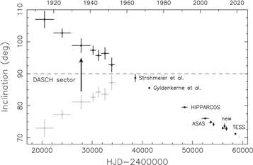
Figure 1. Inclination of the eclipsing binary of HS Hya system determined from the available photometric observations (see also Table 1). Heliocentric Julian Day (HJD) at the bottom abscissa converted to civic years at the upper abscissa. Various historic sources are indicated by labels. The data are shown along with their formal uncertainty (vertical error bar), and the interval of time over which the data were compiled (horizontal line). The pre-1955 data obtained from the DASCH program have been flipped to values larger than 90° to ensure a smooth connection to the results of modern observations (see Section 4). The last symbol (gray arrow), corresponding to TESS sector 35 observations, denotes just the upper limit of the inclination.
Download figure:
Standard image High-resolution imageThird, we also aim at complementing and improving the HS Hya data set itself. For instance, the way how Davenport et al. (2021) divided decades of data from DASCH plates seems to us rather unequal (see their Figure 2). Knowing about the inclination changes, data from some of the longest-spanning intervals of time may provide skewed results. Therefore, while still using the original data from Davenport et al. (2021), we split them into intervals of time spanning, at maximum, a decade (obviously, making sure enough observations are available for our analysis). In this way, we succeed to get more inclination values determined in the first half of the 20th century, which is suitable for our analysis in Section 4. If some of our intervals contain fewer observations, the resulting inclination of the binary orbit simply has a larger formal uncertainty associated and thus does not corrupt our final results. Additionally, our work contains new photometric and spectroscopic observations taken in the past decade. The photometry has been obtained with small-aperture telescopes only, and given the shallow nature of eclipses, the inclination determination was not very accurate (see Table 1). Nevertheless, these data points are of some value in our HS Hya model. The spectroscopic observations merely confirm validity of the previous solution from Torres et al. (1997), helping at this moment just to improve accuracy in determination of the outer orbital period. However, their value may be important in the future, when additional precise spectroscopic observations are eventually available and more ambitious solutions of the the HS Hya orbital and physical parameters are developed.
Most importantly, our model for interpretation of both photometric and spectroscopic data is much more detailed than in Davenport et al. (2021; see the theory presented in Section 3, followed with data analysis in Section 4). This allows us to correct some of their conclusions, such as a tight limit on the precession period in their Table 1, and obtain entirely new results, such as interesting constraints on the mass of the third stellar component in the system or noncoplanarity of the orbital planes in HS Hya.
2. Observations
In the next two sections, we present a brief list of the available photometric and spectroscopic data. Excellent and more detailed overviews could be found in Davenport et al. (2021) for the photometry and Torres et al. (1997) for the spectroscopy parts. Apart from the previously used data sets, we also add our own photometric observations and we analyze archived, but not yet used spectroscopic data obtained in regular operations of ESO telescopes. In order to make our inclination data set as homogeneous as possible, a quality we rate important to justify our results, we reanalyze the whole observational material anew in this paper using a single approach.
2.1. Photometric Data
Given the inclination changes, it is important to split the available data set into segments corresponding to different epochs. The postwar sources were logically parsed into segments published in different papers. The All Sky Automated Survey (ASAS) data were split the same way as in our previous work Zasche & Paschke (2012). On top of what has been included in this work, we also added (i) new data from observations taken in between 2012 and 2014 (some details are given in the Appendix), and (ii) the TESS (Ricker et al. 2015) observations from sector 9, reported in Davenport et al. (2021). Unfortunately, sector 35 observations already reveal no sign of eclipses and thus they can only provide an upper limit on the inclination value. A special care has also been devoted to the important prewar extension of the data from DASCH archive (Davenport et al. 2021). As mentioned above, we experimented with their splitting schemes aiming to collect data from, at maximum, a decade. We ended up with slightly more data points, though dropping data before 1910 where we could not identify a clear eclipsing signal. Our analysis procedure is as follows.
We note that the observations in Gyldenkerne et al. (1975) are of a superior quality in a number of respects: (i) they are numerous; (ii) they are accurate; (iii) they have been taken in four different filters of the Strømgren system; and (iv) perhaps most importantly, they were taken near the epoch of maximum depth of eclipses (i.e., inclination near to 90°). The recent TESS observations rival those of Gyldenkerne et al. (1975) in aspects (i) and (ii), being in fact better in both, but fail to satisfy (iii) and (iv). At their epoch, the eclipses were nearly grazing, thus photometrically very shallow, not allowing to properly describe parameters of the stars in the eclipsing system. We thus consider the set of observations by Gyldenkerne et al. (1975) as a template laboratory to constrain numerous parameters of the stars in the eclipsing binary. These values are then considered fixed, and all other data sets at different epoch are only used to determine the osculating inclination of the binary orbit at that time.
We used the state-of-the-art code PHOEBE (Prša & Zwitter 2005) for our analysis. The results with the template observation set of Gyldenkerne et al. (1975) are basically the same as those published in Zasche & Paschke (2012). We also briefly comment on the third light problem, namely contribution of the third stellar component in the HS Hya system. If significant, it can skew results for the physical parameters of the eclipsing stars in the binary. Ideally, the third light contribution should be solved for as an independent parameter. However, this is problematic for HS Hya because of the number and quality of the available data. Even with the superior set of observations by Gyldenkerne et al. (1975), these authors observed problems in solving the exact value of the third light contribution (setting it though smaller than few percents; see their Section 5). This issue was also discussed by Torres et al. (1997), who also argued for a very small light contribution from the third component. We thus decided to assume, in our lightcurve analyses, zero contribution of the third light. We note that the third star mass constraint derived here in Section 4 would correspond to the third light contribution ≲0.3%. This is an important justification of the consistency of our analysis.
The resulting list of 18 positive data points for inclination of the HS Hya eclipsing binary component over more than a century timespan is summarized in the Table 1, visually also presented in Figure 1.
2.2. Spectroscopic Data
We also reviewed available spectroscopic information about the HS Hya system. We note the data set obtained by Popper (1971) that we decided to reanalyze anew. By far the largest set of spectra was obtained by Torres et al. (1997). In this case we used the original data from this source. Besides this previously published material, we also used new spectra from the ESO archive. In particular, we identified seven exposures from FEROS spectrograph and ten exposures from HARPS. All of them were obtained between 2009 and 2015, hence complementing in this sense the older observations by Popper (1971) and Torres et al. (1997). In all cases, when we analyzed the spectra, we used a well-tested code RaveSpan (Pilecki et al. 2017), using cross-correlation functions and broadening functions as well. Obviously, each time we had to determine radial velocity motion of the stars in the eclipsing binary first (whose only spectral lines are observable). The residuals then contained the information about the binary center-of-mass motion about the common barycenter with the third components, therefore providing information about the outer orbit. We primarily focused on characterization of this signal. The resulting spectroscopic elements are summarized in the Table 2, and again visualized in Figure 2.
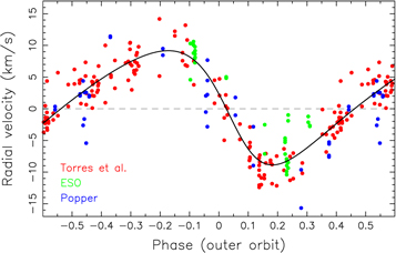
Figure 2. Radial velocity of the eclipsing binary center of mass, after eliminating the much larger signal due to motion of stars in the binary (≃120 km s−1 amplitude) and a small systemic velocity of the whole HS Hya system (≃8 km s−1) from the original velocities derived from spectra. Epochs of the individual measurements mapped onto a phase using ephemeris constants given in Table 2. Three sets of data are merged together: (i) blue symbols from Popper (1971), (ii) red symbols from Torres et al. (1997), and (iii) green symbols based on new observations reported here (FEROS & HARPS instruments at ESO telescopes). More than 40 yr between the first and last observations here may cause inconsistency in determination of the amplitude, because of potentially changing inclination of the outer orbit (Section 4). The black line is a formal best fit using elliptic orbit (see parameters in Table 2).
Download figure:
Standard image High-resolution imageTable 2. Outer Component Orbital Parameters from Compilation of Spectroscopic Data
| Parameter | Value |
|---|---|
| P2 (days) | 190.530 ± 0.015 |
| K2 (km s−1) | 9.02 ± 0.31 |
| e2 | 0.246 ± 0.029 |
| ω2 (deg) | 111.2 ± 7.6 |
| T0 (JD) | 2448047.2 ± 3.4 |
Note. K2 stands for amplitude of the inner binary orbit with respect to the barycenter of the whole system.
Download table as: ASCIITypeset image
The extension of the timespan over which the spectroscopic observations are available by the ESO archive data helps to pin down the period P2 of the outer orbit more accurately then previously possible. The other elements, the amplitude K2 in particular, show a slight differences if compared with results in Torres et al. (1997), generally on a level little larger than the one sigma of their formal solutions. Such a difference is statistically acceptable, however, there might be also conceptual reasons for this discrepancy. Note that the inclination of the outer orbit may change by as much as 6°–7° in between 1971 and 2015 (see, e.g., Figures 6 and 11). This change may affect the amplitude K2 in a noticeable manner (up to ∼5%, say). For this reason, we use the time-localized best spectroscopic data set from Torres et al. (1997) in our analysis at this moment (Section 4.2).
3. Theory
Denote m1a
and m1b
masses of the two stars in the eclipsing binary. Its total and reduced masses are simply M1 = m1a
+ m1b
and μ1 = m1a
m1b
/M1. The third star in the system has mass m2, and thus the total mass is M2 = M1 + m2. Denoting also mean orbital periods P1 of the eclipsing binary and P2 of the third component, we have the corresponding mean motions n1 = 2π/P1 and n2 = 2π/P2. Finally, we assume the orbit of the eclipsing system is circular (e1 = 0), and the eccentricity of the third-star orbit is e2. We also define  .
.
With that notation set, the orbital angular momentum of the binary L1 and motion of the third star L2 are given by

and

where G is the gravitational constant. The value of L1 obviously depends only on the parameters of the inner binary, and L2 is additionally a (nonlinear) function of the unknown mass m2. As long as m2 ≥ 0.4 M⊙, L2/L1 ≥ 2.85 for the HS Hya system. Obviously, both angular momenta are vectorial quantities L 1(0) = L1 l 1(0) and L 2(0) = L2 l 2(0), where the unit vectors l 1(0) and l 2(0) define orientation of the respective orbital planes at an arbitrary time origin at the epoch T0. In principle, each of the unit vectors could be expressed using two angular parameters. But with the available data set, we can arbitrarily set one of them to be zero. In particular, we may define

and

where i1 and i2 and orbital inclinations of the eclipsing binary and third motion with respect to the sky-plane at T0. The only other needed parameter is Ω2, namely nodal longitude of the third motion in a system where Ω1 = 0 for the eclipsing binary. The total angular momentum of the system
L
= L
l
=
L
1(0) +
L
2(0) is a conserved quantity (neglecting angular momentum stored in rotational motion of the components). The initial data at T0 provide its magnitude L and direction
l
. It is also useful to introduce the mutual angle J between the orbital plane of the eclipsing binary and the orbital plane of the third-body motion. Using our variables we have  .
.
It is useful, at this moment, to review the principal solved-for parameters of our approach. These are (i) the mass of the third component m2, (ii) the inclination i1 of the eclipsing binary at T0, and (iii) the corresponding angular parameters i2 and Ω2 of the third-component motion at T0. We assume the periods P1 and P2 be known accurately enough, as well as the masses m1a and m1b of the components in the eclipsing binary (e.g., Torres et al. 1997; Zasche & Paschke 2012). The fair enough knowledge of the stellar masses in the eclipsing binary assumes spectroscopic observations providing well-resolved lines of both components, determination of the radial velocity amplitude of the P1-periodic component, and a solid determination of the inclination i1 at their epoch. The data of Torres et al. (1997), with i1 corrected in Zasche & Paschke (2012), meet approximately these conditions. However, when a lot of spectroscopic observations from different epochs are available, one may be more ambitious. In particular, both masses m1a and m1b may also be included in an extended analysis of all data altogether. In Section 4.2 we test this approach with the currently available, but still limited spectroscopic data by letting m1a to be an additional solved-for parameter (assuming the ratio q = m1b /m1a known exactly). The model thus contains altogether four unknown, to-be-fitted parameters, in its basic form, or five, when m1a is also let free. The choice of T0 is arbitrary. It may be a barycenter of the observations, or the epoch of the smallest-uncertainty observation (in what follows, we actually use this option and T0 is the epoch of the TESS observations). Even if the latter, i1 is still a free parameter of the model. Obviously, it must be close to the observed inclination at that epoch, but a good fit of the other observations may require their small difference.
In the simplest point-mass model, we may restrict to the secular perturbations, neglecting short- and long-periodic effects, and consider the quadrupole part of the interaction potential. The latter approximation is justified when the period ratio P1/P2 has a small value (as in the HS Hya case), in other words when the triple system is not too compact. Additionally, since m1a is not too different from m1b , the role of the odd interaction multipole terms (such as the octupole) is very small (e.g., Soderhjelm 1984). If justified, the secular quadrupolar model for a hierarchical triple is a very useful approximation, because it admits a simple analytical solution when (i) e1 = 0 and (ii) J is small enough (approximately ≤40° or ≥140°; e.g., Soderhjelm 1982; Farago & Laskar 2010). The zero eccentricity of the eclipsing binary is a stable equilibrium solution, and J also remains constant. The orbital plane dynamics is expressed by a simple behavior of the unit vectors of the angular momenta. Both l 1(t) and l 2(t) uniformly precess about the conserved direction of the total angular momentum l , rolling on fixed conic surfaces with constant opening angles. The precession frequency ν is given by (e.g., Soderhjelm 1975; Breiter & Vokrouhlický 2015)
where

Note that ν is a nonlinear function of all four parameters (m2, i10, i20, Ω20) of the model, the angles expressed at the reference epoch T0. A simple vectorial algebra then provides (relation sometimes also known as the Rodrigues' rotation formula)

with α = ν(t − T0) (a similar formula holds also for
l
2(t)). The inclination i1(t) of the eclipsing system is then simply  , where
  . A similar formula applies to the orbit of the third star in the system using a simple change of index 1 to 2.
Our model is equivalent of that used in Zasche & Paschke (2012), based on earlier formulation of Soderhjelm (1975). However, we would argue that the current version has the advantage to be more straightforwardly connected to the parameters of interest. Indeed, Zasche & Paschke (2012) fitted the inclination series i1(t) of the eclipsing system using an analytic model with the following set of four parameters: (i)  , the inclination of the constant invariable plane of the triple, (ii)
  , inclination of the eclipsing binary with respect to the invariable plane, (iii) ν, precession frequency, and (iv) τ, the epoch when i1(t) has a maximum value. Of these, only the latter two are observationally related. Our remapping to the observable inclination i1 of the eclipsing binary at T0, the inclination i2 of the orbital plane of the third body (potentially relevant for interpretation of the spectroscopic observations), and directly mass m2 of the third body looks to us more useful. Additionally, the simple formula (7) is more general, as it directly provides also the evolution of the sky-plane nodal longitude of the eclipsing binary. It may thus easily serve to obtain the sky-plane projection of the binary orbit or the third component, an information relevant for potential interferometric observations (if available).
The simple analytic solution (7) is not valid in the point-mass model when  is smaller than some critical value of about ≃0.77 (or J near 90°; see, e.g., Soderhjelm 1982; Farago & Laskar 2010). This is the well-known Kozai–Lidov regime. However, in the situation when the triple system contains sufficiently close eclipsing binary (again, such as the HS Hya case), worries of a more complicated solution do not apply. This is because the tidal integration of the stars in the binary produce strong-enough dynamical effects, in particular fast-enough precession of the orbital pericenter, which halts the Kozai–Lidov oscillations (e.g., Soderhjelm 1984). Therefore, while it is useful to check the J angle in the results, the solutions may well apply for even large J angles provided the stars in the eclipsing binary interact at some minimum level (a condition required for the system long-term stability anyway).
Finally, while the data fitting is performed using the simple analytical model outlined above, we note that we also made sure the solution holds using a full-fledged numerical model. We used a point-mass configuration and Jacobi coordinates (e.g., Soderhjelm 1982) with tidal interaction effects included (e.g., Soderhjelm 1984). This is a useful check, because it allows us to verify that the neglected effects, in particular the short- and long-period perturbations and higher-multipole interaction terms, are not needed for the data set we have (i.e., inclination i1 of the eclipsing binary with characteristic uncertainty of a fraction degree or so). Additionally, it also justifies our model for arbitrary mutual inclination J of the two orbits.
For sake of completeness, we also provide information about precession rate  of pericenter of the outer component in the triple system. This additional secular effect in the system is independent from the orbital plane dynamics described in Equation (7). Remaining in the framework of the secular, quadrupole-interaction model, one has (e.g., Soderhjelm 1975; Breiter & Vokrouhlický 2015)
Because  depends on a steeper power of the frequency ratio n2/n1 than ν, the corresponding period
  is typically longer than Pν
= 2π/ν, notably period of angular momenta
l
1 and
l
2 precession about
l
. Note that Pν
is also the period of inclination i1 and i2 variations.
is typically longer than Pν
= 2π/ν, notably period of angular momenta
l
1 and
l
2 precession about
l
. Note that Pν
is also the period of inclination i1 and i2 variations.
4. Results
We start our analysis by using the photometric data set only. This serves as a good test of the method outlined in Section 3, and also provides a point of reference for a more complete solution, in which we include additional constraints from the spectroscopic data.
4.1. Solution Using Photometric Data Set Only
Results from the analysis of the photometric observations discussed in Section 2.1 are formally organized in triples (tj , i1,j , Δi1,j ), with j = 1,...,Ndata = 18, where tj is the epoch at which inclination i1,j was determined with an uncertainty Δi1,j (see Table 1). We recall that the pre-1995 data from DASCH have been mirrored over 90° as indicated on Figure 3 and also resolved originally by Davenport et al. (2021). In fact, we ran simulations for both possibilities, flipping and not flipping the early inclination data, and found no consistent and statistically acceptable solutions in the latter case.
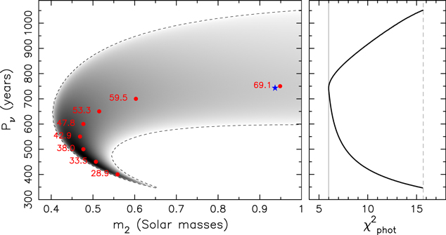
Figure 3. Left: distribution of solutions for which  projected onto the plane of mass m2 (abscissa) and precession period Pν
(ordinate); configurations corresponding to the prograde motion of the third star used here (i.e., J < 90°). Solution density is indicated by greyscale, white for no possible solution, black for the largest number of solutions. The dashed lines delimit the zone of acceptable solutions. The blue star at m2 = 0.94 M⊙ and Pν
= 742 yr shows location of the best-fitting solution with
projected onto the plane of mass m2 (abscissa) and precession period Pν
(ordinate); configurations corresponding to the prograde motion of the third star used here (i.e., J < 90°). Solution density is indicated by greyscale, white for no possible solution, black for the largest number of solutions. The dashed lines delimit the zone of acceptable solutions. The blue star at m2 = 0.94 M⊙ and Pν
= 742 yr shows location of the best-fitting solution with  . The red dots are locations of the solutions with the lowest
  value for constant Pν
in between 400 and 750 yr with 50 yr increment. The adjacent red labels are the values of J, i.e., the mutual angle between the orbital planes of the inner binary and outer star. Right: the minimum
value for constant Pν
in between 400 and 750 yr with 50 yr increment. The adjacent red labels are the values of J, i.e., the mutual angle between the orbital planes of the inner binary and outer star. Right: the minimum  (abscissa) for a given Pν
value (ordinate). The dashed vertical line is the limit for accepted solutions
(abscissa) for a given Pν
value (ordinate). The dashed vertical line is the limit for accepted solutions  , the solid vertical line is the best achieved value
  .
.
Download figure:
Standard image High-resolution imageFor sake of simplicity of this initial test, our model optimizes a minimum set of parameters, considering the remaining of them to be constant. These fixed parameters are as follows: (i) masses m1a
= 1.31 M⊙ and m1a
= 1.27 M⊙, based on spectroscopic data of Torres et al. (1997) with a correction of Zasche & Paschke (2012), who used appropriate inclination i1 at the epoch of spectroscopic observations, (ii) orbital periods P1 = 1.568 days and P2 = 190.53 days, and (iii) e2 = 0.25 (Section 2 and Torres et al. 1997). The reference epoch of the model coincides with the TESS observations, namely  , and we consider four-dimensional space (m2, i10, i20, Ω20) of solved-for parameters. Here, i10 = i1(T0), i20 = i2(T0) and Ω20 = Ω2(T0). The goodness of the fit is measured using a standard χ2 metric defined as

where  is provided by Equation (7). Obviously, the intuition tells us that acceptable fits must have
  (acknowledging four degrees of freedom of the solved-for parameters). However, we use slightly more involved criterion based on assumption of Gaussian distribution of uncertainties of both data and parameters (strictly speaking not really satisfied, but in fact providing similar results to those obtained with a simple guess above). Our procedure is as follows. We seek the best-fitting solution in the parameter space (m2, i10, i20, Ω20) and evaluate its
  value. We verify that
  is sufficiently small to be statistically acceptable (we use criterion set by a value of the incomplete gamma function discussed in Section 15.2 of Press et al. 2007). Then, we determine a hyper-volume
  in the parameter space characterized by
  . With four degrees of freedom, a value Δχ2 = 9.7 would characterize a 95% confidence zone in the parametric space (again, if strictly speaking Gaussian statistics is satisfied; see Section 15.6 of Press et al. 2007). In case of five degrees of freedom, the model setup used in the next Section 4.2, we need Δχ2 = 11.3. Projection of
  onto model parameters helps us to characterize their plausible values and the 95% confidence level range.
We start discussing results for a case when the third component in HS Hya moves in a prograde sense, i.e., J < 90° in Section 3. Figure 3 shows projection of  onto a plane defined by m2 and Pν
. In an ideal, Gaussian world,
onto a plane defined by m2 and Pν
. In an ideal, Gaussian world,  would be a four-dimensional hyper-ellipsoid and any projection onto a two-dimensional plane would be simply an ellipse. Here we see these conditions are not exactly satisfied. Instead, the projection of
  has a complex shape and, in fact, exceeds the monitored m2 ≤ 1 M⊙ range. In the same time, Pν
may also span a wide range of values from ≃350 yr to more than 1000 yr. This is because the course of data i1,j
at tj
in Figure 1 does not really show evidence of periodic dependence with a well-defined periodicity. The red symbols with associated labels provide J values for specific solutions with fairly good values of
has a complex shape and, in fact, exceeds the monitored m2 ≤ 1 M⊙ range. In the same time, Pν
may also span a wide range of values from ≃350 yr to more than 1000 yr. This is because the course of data i1,j
at tj
in Figure 1 does not really show evidence of periodic dependence with a well-defined periodicity. The red symbols with associated labels provide J values for specific solutions with fairly good values of  . They range from ≃25° to nearly 70°. The fact that none of the acceptable solutions has very low value of J, i.e., near coplanar configuration, is required by a large observed change of the i1,j
values. The formally best-fitting solution–the blue star in Figure 3–has m2 = 0.94 M⊙ and Pν
= 742 yr.
. They range from ≃25° to nearly 70°. The fact that none of the acceptable solutions has very low value of J, i.e., near coplanar configuration, is required by a large observed change of the i1,j
values. The formally best-fitting solution–the blue star in Figure 3–has m2 = 0.94 M⊙ and Pν
= 742 yr.
Interestingly, there exist also solutions fitting the photometric data for which the third star moves in a retrograde sense, namely J > 90°. Figure 4 shows their distribution in the m2 and Pν plane of parameters. The statistical quality of the best-fitting solution is equivalent to the prograde counterpart, and also the general features of the distribution of acceptable solutions is similar. The only difference is a slight shift of the Pν values to little longer periods.
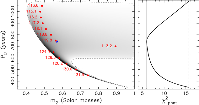
Figure 4. The same as in Figure 3, but now for configurations in which the motion of the third component in HS Hya system is retrograde (i.e., J > 90°). The best-fitting solution is now at m2 = 0.57 M⊙ and Pν
= 742 yr, having again  .
.
Download figure:
Standard image High-resolution imageOverall, our solution has a close similarity to those in the Appendix D in Juryšek et al. (2018). Clearly, the available photometric data of HS Hya themselves are not able to significantly constrain neither the parameters defining its orbital architecture nor the mass m2 of the third stellar component in the system. The only solid limit is m2 > 0.4 M⊙, simply because perturbation from a less massive components is incompatible with so large (observed) variations of the inclination i1 of the eclipsing binary.
4.2. Solution Using Both Photometric and Spectroscopic Data
Luckily, there is more than photometry available for the HS Hya system. In particular, Popper (1971) and Torres et al. (1997) acquired a wealth of spectroscopic observations, and here we added few more in Section 2.2. They are of a fundamental importance, because they were able to tell us some basic information about the orbit of the third component in the system: (i) its orbital period P2 ≃ 190.53 days, and (ii) its eccentricity e2 ≃ 0.25. In the same time, absence of identifiable signal of the third star in the spectra sets an upper limit on its mass, approximately 0.6 M⊙ (see Table 4 and related discussion in Torres et al. 1997). It is this complementary information that allows the analysis of HS Hya system be more complete than for systems treated by Juryšek et al. (2018). In what follows we seek the way how the quantitative results from the spectroscopic observations may be used in our method to better constrain parameters of the HS Hya system.
Here we limit ourselves to the spectroscopic data obtained by Torres et al. (1997) at the Harvard-Smithsonian Center for Astrophysics. This is for two reasons: (i) it is the most complete homogeneous set of observations allowing to characterize parameters of the third component, and (ii) it has been obtained in a reasonably short interval of time (1989–1996), in which we may consider inclinations i1 and i2 approximately constant. We thus complement the inclination i1 data set, obtained by photometric observations and used in Section 4.1, by two data points resulting from analysis of spectroscopic observations in Torres et al. (1997; first column in their Table 3):
- 1.Constraint C1: denote
 the projected mass of the heavier component in the eclipsing system. Then m1a,proj,obs(ts
) = 1.2404 M⊙ with an uncertainty Δm1a,proj,obs =0.0078 M⊙. The mass ratio q in the eclipsing binary is considered fixed, namely q = m1b
/m1a
= 0.9694 (determined with better then 0.4% accuracy).
the projected mass of the heavier component in the eclipsing system. Then m1a,proj,obs(ts
) = 1.2404 M⊙ with an uncertainty Δm1a,proj,obs =0.0078 M⊙. The mass ratio q in the eclipsing binary is considered fixed, namely q = m1b
/m1a
= 0.9694 (determined with better then 0.4% accuracy). - 2.Constraint C2: denote the projected semimajor axis of the third component motion, where the semimajor axis of the outer orbit is given by the Kepler's third law . Then a2,proj,obs(ts
) =34.7 R⊙ with an uncertainty Δa2,proj,obs = 1.1 R⊙.

Both constraints are assigned to ts = 1993.0, mid epoch of the spectroscopic observations reported in Torres et al. (1997). The target χ2 function of the optimization consists of the photometry part in Equation (9), extended by
corresponding to results from the spectroscopic observations, thus:  . In spite of more data in
  , we do not use any specific weighting scheme in favor of the only two constraints in
  . The space of the solved-for parameters is now five dimensional and contains (m1a
, m2, i10, i20, Ω20). In our approach, we first seek the minimum value
. The space of the solved-for parameters is now five dimensional and contains (m1a
, m2, i10, i20, Ω20). In our approach, we first seek the minimum value  of the target function in the parameter space, and then determine hyper-volume
  characterized by
  , where now Δχ2 = 11.3 (Press et al. 2007).
We start again by analyzing configurations in which the third star moves in a prograde sense, i.e., J < 90°. Figure 5 shows the projection of  onto the plane of m2 and Pν
, together with gray-scale indicated density of admissible solutions. This may be directly compared with Figure 3, in which only photometric data were used. In spite of one more degree of freedom of the space of solved-for parameters, namely m1a
, both m2 and Pν
are now quite better constrained. We find this is principally a consequence of the constrained C2; this is because when fixing m1a
= 1.31 M⊙ as above, we obtained very similar result to what is seen in Figure 5. The best-fitting solution has
onto the plane of m2 and Pν
, together with gray-scale indicated density of admissible solutions. This may be directly compared with Figure 3, in which only photometric data were used. In spite of one more degree of freedom of the space of solved-for parameters, namely m1a
, both m2 and Pν
are now quite better constrained. We find this is principally a consequence of the constrained C2; this is because when fixing m1a
= 1.31 M⊙ as above, we obtained very similar result to what is seen in Figure 5. The best-fitting solution has  , satisfactorily smaller than Nobs − 5 = 15. Its position on Figure 5 is marked by the blue star symbol. The green star symbol identifies the best-fitting solution in the tail of shorter Pν
values; it has χ2 = 9.74, quite worse than
, satisfactorily smaller than Nobs − 5 = 15. Its position on Figure 5 is marked by the blue star symbol. The green star symbol identifies the best-fitting solution in the tail of shorter Pν
values; it has χ2 = 9.74, quite worse than  , but still statistically acceptable value. Figure 6 shows model prediction for i1 and i2 time dependence for the late 1800th until nearly 2400. The data shown here allow us appreciate how the model fits the photometric data (left panels and red symbols with error bars). In the same time, we can see prediction for the future course of both i1 and i2, whose common periodicity is Pν
. Because of their different values, we note that the best-fitting solution would predict HS Hya will become an eclipsing system again just shy of 2200 (in agreement with Davenport et al. 2021), but the model in the right panel of Figure 5 gets the epoch at ≃2110. The two solutions also differ significantly in a prediction of the possible binary eclipses by the third component is the HS Hya system (note this requires i2 very close to 90°). The best-fitting solution (left panel on Figure 5) does not allow such a configuration, since i2 is always larger than ≃965, while the solution in the right panel on Figure 5 predicts this possibility for about 2175. These two examples indicate that there is still quite large variability of predicting such events for HS Hya. Some other parameters are, however, quite better constrained.
, but still statistically acceptable value. Figure 6 shows model prediction for i1 and i2 time dependence for the late 1800th until nearly 2400. The data shown here allow us appreciate how the model fits the photometric data (left panels and red symbols with error bars). In the same time, we can see prediction for the future course of both i1 and i2, whose common periodicity is Pν
. Because of their different values, we note that the best-fitting solution would predict HS Hya will become an eclipsing system again just shy of 2200 (in agreement with Davenport et al. 2021), but the model in the right panel of Figure 5 gets the epoch at ≃2110. The two solutions also differ significantly in a prediction of the possible binary eclipses by the third component is the HS Hya system (note this requires i2 very close to 90°). The best-fitting solution (left panel on Figure 5) does not allow such a configuration, since i2 is always larger than ≃965, while the solution in the right panel on Figure 5 predicts this possibility for about 2175. These two examples indicate that there is still quite large variability of predicting such events for HS Hya. Some other parameters are, however, quite better constrained.

Figure 5. The same as in Figure 3, but now the criterion of solution acceptance is  , namely both photometric and spectroscopic data are taken into account. The best-fitting solution (blue star) has m2 = 0.582 M⊙ and Pν
= 700 yr, and corresponds to
, namely both photometric and spectroscopic data are taken into account. The best-fitting solution (blue star) has m2 = 0.582 M⊙ and Pν
= 700 yr, and corresponds to  . In this case we also treated m1a
as a free parameter; the best-fitting solution has m1a
= 1.313 M⊙. The green star denotes a solution corresponding to the second minimum of χ2(Pν
) shown on the right panel. The value χ2 = 9.74 is slightly worse than
. In this case we also treated m1a
as a free parameter; the best-fitting solution has m1a
= 1.313 M⊙. The green star denotes a solution corresponding to the second minimum of χ2(Pν
) shown on the right panel. The value χ2 = 9.74 is slightly worse than  , but still statistically acceptable. It corresponds to m1a
= 1.316 M⊙, m2 = 0.526 M⊙ and Pν
= 433 yr.
, but still statistically acceptable. It corresponds to m1a
= 1.316 M⊙, m2 = 0.526 M⊙ and Pν
= 433 yr.
Download figure:
Standard image High-resolution image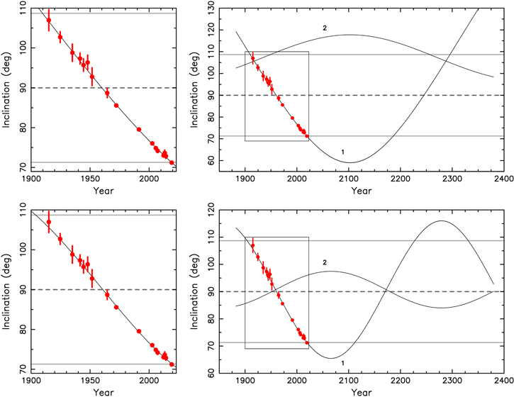
Figure 6. Inclination i1 (label 1) and i2 (label 2) of the inner (binary) and outer-component orbits of HS Hya over the next few centuries (the abscissa in years). Red symbols are data with uncertainties determined in Section 2.1. Left panels provide a zoom on the century of inclination data (depicted using the rectangle on the right panels) and show only the i1 values. Top panels for the best-fitting model from Figure 5 (blue star) having m1a
= 1.313 M⊙, m2 = 0.582 M⊙, Pν
= 700 yr, and J = 587. Bottom panels for an alternative, little worse but still statistically acceptable solution, with m1a
= 1.316 M⊙, m2 = 0.526 M⊙, Pν
= 433 yr, and J = 319 (green star in Figure 5). The gray horizontal lines at inclinations 713 and 1087 delimit the zone of i1 values for which the inner binary is eclipsing. The third component is capable to eclipse the inner binary when i2 values are in a very narrow interval of ≃±1° near 90° (dashed line). The bottom-panel solution thus allows this configuration in about 2175, but in the top-panel solution, the third component never eclipses the inner binary.
Download figure:
Standard image High-resolution imageFigure 7 shows probability density distribution of the stellar masses involved in our optimization procedure: (i) m1a
of the heavier component in the eclipsing binary, and (ii) m2 of the third component in the HS Hya system. Both functions are obtained by projecting all solutions contained in  , and the ordinate is normalized such that the integral over m1a
and m2 is unity (assumed solar mass as units). The full width results, corresponding to the 95% confidence level range, may be expressed as
, and the ordinate is normalized such that the integral over m1a
and m2 is unity (assumed solar mass as units). The full width results, corresponding to the 95% confidence level range, may be expressed as  and
and  . Both are quite interesting. For instance the uncertainty of m1a
is only three times larger than the uncertainty of the projected mass m1a, proj (constraint C1 above). This is because uncertainty in m1a
is also subject to the correlated uncertainty in i1 at ts
, but at the same time, inclination data constrain the admissible value i1(ts
) fairly well. Our median value confirms the solution in Table 3 of Zasche & Paschke (2012) but additionally extends it by a realistic uncertainty range. Given the high accuracy in the ratio q of stellar masses in the eclipses binary, we can also conclude that our results imply
. Both are quite interesting. For instance the uncertainty of m1a
is only three times larger than the uncertainty of the projected mass m1a, proj (constraint C1 above). This is because uncertainty in m1a
is also subject to the correlated uncertainty in i1 at ts
, but at the same time, inclination data constrain the admissible value i1(ts
) fairly well. Our median value confirms the solution in Table 3 of Zasche & Paschke (2012) but additionally extends it by a realistic uncertainty range. Given the high accuracy in the ratio q of stellar masses in the eclipses binary, we can also conclude that our results imply  . Perhaps even more interesting is the solution for m2, which sets its M- or K-dwarf type star. Recall that our solution is derived uniquely by the dynamical constraints, and does not employ an independent argument from absence of the third component in HS Hya total luminosity. Yet, this agreement represents a good justification of our results.
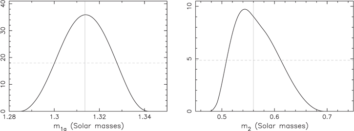
Figure 7. Probability density distribution of solution for mass m1a
in the HS Hya eclipsing binary (left panel) and mass m2 of the third component (right panel). The available data set from both photometric and spectroscopic observations used. The nonzero values correspond to the projection of five-dimensional parameter-space zone  containing all admissible solutions within 95% confidence limit. These results assume prograde motion of the third star in the system (i.e., J < 90°). The vertical solid line is the median value of the distribution, and the horizontal dashed line is the half-maximum level.
Download figure:
Standard image High-resolution imageFigure 8 shows the probability density distribution of our solution for the precession period Pν
(left panel) and mutual inclination J of the inner and outer orbits of HS Hya system (right panel); normalization of the ordinate uses units at the abscissa. The 95% confidence range can be formally expressed as  yr and
  degrees, where the highlighted value is median of the distribution. These intervals are quite large and result from absence of clear periodicity of the inclination data i1,j
(Figure 1). Nevertheless, most of the Pν
values are in between 600 and 800 yr, while the most likely values of J are in between 55° and 65°. The high inclination of the outer orbit is notable and corrects conclusions from several earlier studies (e.g., Davenport et al. 2021). We recall that this results is not in conflict with long-term stability of the HS Hya system via Kozai–Lidov process. This is because the expected tidal interaction of the stars in the compact inner binary produces fast precession of their pericenter, which halts onset of its eccentricity by gravitational perturbation due to the third component (one may recall the most classical high-inclination Algol system with basically J = 90°, see Baron et al. 2012). We explicitly verified this conclusion by using the simple nondissipative tidal model quoted in Soderhjelm (1984). For instance, the best-fitting solution shown in the top panels of Figure 6 that has J = 587 is stable when the parameter Dt
≥ 10−5 (taking into account just the tidal deformation of the binary components). Assuming equal properties of both stars in the eclipsing binary, this translates to k(2) ≥ 0.012 for their apsidal motion constant (a justifiable value, e.g., Claret & Gimenez 1995).
degrees, where the highlighted value is median of the distribution. These intervals are quite large and result from absence of clear periodicity of the inclination data i1,j
(Figure 1). Nevertheless, most of the Pν
values are in between 600 and 800 yr, while the most likely values of J are in between 55° and 65°. The high inclination of the outer orbit is notable and corrects conclusions from several earlier studies (e.g., Davenport et al. 2021). We recall that this results is not in conflict with long-term stability of the HS Hya system via Kozai–Lidov process. This is because the expected tidal interaction of the stars in the compact inner binary produces fast precession of their pericenter, which halts onset of its eccentricity by gravitational perturbation due to the third component (one may recall the most classical high-inclination Algol system with basically J = 90°, see Baron et al. 2012). We explicitly verified this conclusion by using the simple nondissipative tidal model quoted in Soderhjelm (1984). For instance, the best-fitting solution shown in the top panels of Figure 6 that has J = 587 is stable when the parameter Dt
≥ 10−5 (taking into account just the tidal deformation of the binary components). Assuming equal properties of both stars in the eclipsing binary, this translates to k(2) ≥ 0.012 for their apsidal motion constant (a justifiable value, e.g., Claret & Gimenez 1995).
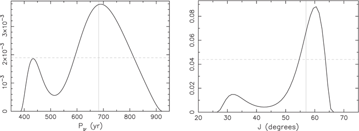
Figure 8. Probability density distribution of solution for precession period Pν
and mutual inclination J < 90° of inner and outer orbits of the HS Hya system. The available data set from both photometric and spectroscopic observations used. The nonzero values correspond to the projection of the five-dimensional parameter-space zone  containing all admissible solutions within 95% confidence limit. The vertical solid line is median value of the distribution, and the horizontal dashed line is the half-maximum level.
Download figure:
Standard image High-resolution imageFinally, Figure 9 shows probability density distribution for the epoch in which our model predicts onset of eclipses in the HS Hya anew. The 95% range can be written as  . The median value is close to the solution in Davenport et al. (2021), but the range is much larger. The earliest solution, though not very likely, could happen still in this century. The most likely values are in between 2100 and 2250.
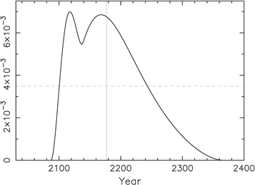
Figure 9. Solution for the forthcoming onset of the inner binary eclipses in HS Hya expressed by a probability density distribution resulting from the modeling fitting the available photometric and spectroscopic data. The vertical line denotes the medium value for which the cumulative probability is 0.5, and the horizontal dashed line is the half-maximum level.
Download figure:
Standard image High-resolution imageNext, we recall there is also a possibility for HS Hya architecture in which the third component moves in a retrograde sense (i.e., J > 90°). We extended the solution from Section 4.1, based on photometric data, by the two constraints C1 and C2 discussed above. Figure 10 shows again the projection of the 95% confidence level hyper-volume  onto the plane m2 and Pν
, together with a gray-scale indication of the density of possible solutions. As in the case of prograde solutions, the spectroscopic data importantly shrunk the zone of admissible solutions (compare with Figure 4). The formally best-fitting solution has
onto the plane m2 and Pν
, together with a gray-scale indication of the density of possible solutions. As in the case of prograde solutions, the spectroscopic data importantly shrunk the zone of admissible solutions (compare with Figure 4). The formally best-fitting solution has  (blue star on Figure 10), statistically equivalent to the best prograde solution. The fitted stellar masses m1a
= 1.313 M⊙ and m2 = 0.581 M⊙ are the same as in the prograde-solution space, the precession period is slightly longer Pν
= 742 yr. Figure 11 shows time dependence of i1 and i2 for the best-fitting retrograde solution. The longer Pν
values makes its periodicity not apparent over the five centuries shown.
(blue star on Figure 10), statistically equivalent to the best prograde solution. The fitted stellar masses m1a
= 1.313 M⊙ and m2 = 0.581 M⊙ are the same as in the prograde-solution space, the precession period is slightly longer Pν
= 742 yr. Figure 11 shows time dependence of i1 and i2 for the best-fitting retrograde solution. The longer Pν
values makes its periodicity not apparent over the five centuries shown.
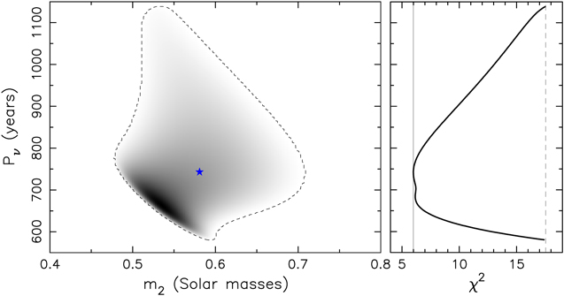
Figure 10. The same as in Figure 5, but now for configurations with the third star moving in a retrograde sense. The best-fitting solution (blue star) has m2 = 0.581 M⊙ and Pν
= 742 yr, and corresponds to  . In this case we also treated m1a
as a free parameter; the best-fitting solution has m1a
= 1.313 M⊙.
. In this case we also treated m1a
as a free parameter; the best-fitting solution has m1a
= 1.313 M⊙.
Download figure:
Standard image High-resolution image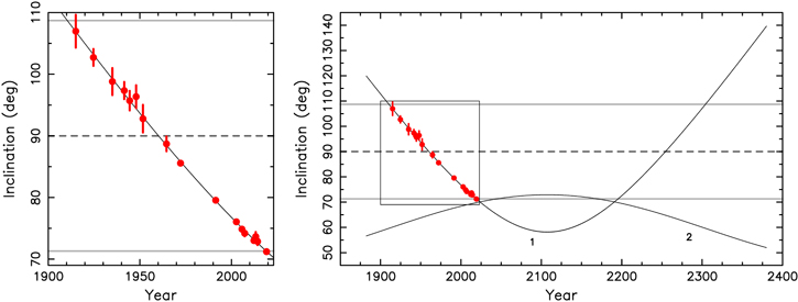
Figure 11. Inclination i1 (label 1) and i2 (label 2) of the inner (binary) and outer-component orbits of HS Hya over the next few centuries (the abscissa in years). Red symbols are data with uncertainties determined in Section 2.1. The left panel provides a zoom onto the century of data (see also the rectangle on the right panel) with only i1 shown. The solid lines are for the best-fitting model from Figure 5 (blue star) having m1a
= 1.313 M⊙, m2 = 0.581 M⊙, Pν
= 742 yr and J = 1312. As in the left panel of Figure 6, the third star never eclipses the inner binary, because the maximum i2 value is about 729.
Download figure:
Standard image High-resolution imageThe solution for m1a
is very similar to what is seen on the left panel of Figure 7, giving  (implying the same solution for m1b
as before). This is again a direct consequence of the constraint C1. Note that the inclination i1,j
data set is fairly solid near the epoch ts
= 1993.0 of the spectroscopic data, and thus does not allow too much variation in admissible inclination i1 value. Solutions for other parameters of interest, third component mass m2, precession period Pν
and the mutual angle J of inner and outer orbits, are now shown in the three panels of Figure 12. The full-range solution
(implying the same solution for m1b
as before). This is again a direct consequence of the constraint C1. Note that the inclination i1,j
data set is fairly solid near the epoch ts
= 1993.0 of the spectroscopic data, and thus does not allow too much variation in admissible inclination i1 value. Solutions for other parameters of interest, third component mass m2, precession period Pν
and the mutual angle J of inner and outer orbits, are now shown in the three panels of Figure 12. The full-range solution  matches that for the prograde configurations, and it is very satisfactory in view of the independent constraint from direct nondetection of the third component in the system. Precession period
  yr is now shifted to slightly longer values, as expected for retrograde configurations, while the orbital-plane mutual angle
  has less of the asymmetry seen for the prograde configurations. Because of longer Pν
values, the retrograde solution predicts onset of future HS Hya eclipses to
has less of the asymmetry seen for the prograde configurations. Because of longer Pν
values, the retrograde solution predicts onset of future HS Hya eclipses to  , with basically no solutions before 2150.
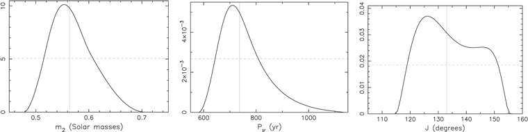
Figure 12. Solution for the mass m2 of the third component in the HS Hya system (left panels), precession period Pν (reflected in periodicity of i1 and i2; middle panels) and mutual angle J of the orbital planes, when both photometric and spectroscopic constraints are taken into account, and J is restricted to retrograde configurations (i.e., J > 90°). The plotted curve is a probability density distribution of the corresponding parameter within its 95% confidence interval. The vertical line denotes the medium value for which the cumulative probability is 0.5, the horizontal dashed line is half-maximum level.
Download figure:
Standard image High-resolution image
5. Discussion and Conclusions
Quantifying the range of admissible inclination i1 values at the time of spectroscopic observations, we could set realistic limits on the masses m1a and m1b of the stellar components in the eclipsing binary of HS Hya. The constraint on the mass m2 on the unseen stellar companion is even more interesting result from this study. Using just a dynamical model, we found it ranges from 0.47 to 0.68 M⊙. This is in a satisfactory agreement with absence of the third light in the HS Hya system at the <1% level.
The second principal result concerns the noncoplanarity of the inner and outer orbits of the HS Hya system (Figures 8 and 12). Here we would like to remind that the perception of a necessity to have a near-to-coplanar configuration in hierarchic triples may not be justified. Instead, modeling of Sterzik & Tokovinin (2002) suggests these triple systems may initially form in a nearly isotropic fashion as far as their orbital architecture is concerned if gravitational N-body interactions dominate their early formation (see, however, more complex formation channels involving gaseous environment in the birth cluster that may result in a more planar configurations of compact systems at preference, e.g., Tokovinin 2017, 2021). Subsequent evolution, dominated by an interplay between the gravitational interactions and tidal effects, may modify the initial orbital arrangement. The Kozai–Lidov mechanism may cause instability of some of the high-J initial systems. However, the degree of elimination of this category depends on the period of the inner binary. As shown by (Fabrycky & Tremaine 2007, their Figure 7), systems which start with sufficiently short periods P1 have a good chance to survive stable even if starting in a high-J state. Since the inner binary in the HS Hya system belongs to this class, its present large J value may not be in conflict with theoretical predictions.
HS Hya system will become eclipsing beyond the year 2100, and most likely only at the end of the 22nd century. However, useful information about this interesting triple system may be obtained much earlier through spectroscopic observations. Accurate-enough data may continue tracking the evolution of the inclination i1 of the binary, and eventually also the inclination i2 of the third-component orbit. Both may be constrained through fitting the amplitude of the respective radial velocity signal with P1 and P2 periods. For instance, the presently best-fitting prograde model in Figure 8 predicts i1 ≃ 683 by the end of this decade and another two degrees smaller in 2040. The radial velocity amplitude at the P1 period should thus decrease by more than 5% compared to the value determined by Torres et al. (1997). As the masses m1a
and m1b
are already constrained at the 2% level, these spectroscopic measurements should provide valuable information about i1 at those epochs. Similar measurement of i2 from radial velocity amplitude at the P2 period, see our constraint C2 in Section 4.2, may be more challenging, as it would require very precise spectroscopic observations spanning half a year. This is because the radial velocity amplitude at the P2 period is more than ten times smaller than that at the P1 period and variations of i2 are smaller than i1. Another potential dynamical effect one would hope to detect using the future spectroscopic observations is the advance in the outer orbit pericenter. However, the acceptable configurations predict, at maximum, a drift rate of a few degrees per decade (see also Equation (8)). The detection of this effect thus needs to wait for good spectroscopic data in the second half of this century only. In any case, strengthening the model with more data would be certainly useful and may allow more ambitious fits than here (such as fitting both masses m1a
and m1b
independently, or further constraining the solved-for parameters more tightly).
The question of prograde or retrograde motion of the third component in the HS Hya system could be resolved by high-quality interferometric observations. However, it is yet to be seen how challenging they are today. The two stars in the former eclipsing binary separate at a maximum angular distance of only ≃0.35 mas. Unfortunately, the ∼8.1 visual magnitude of the HS Hya system is likely too faint to perform accurate enough measurement of such a tiny angular distance with the currently existing instruments. The maximum extent of the outer-star orbit is comfortably large, more than 9 mas, however the low luminosity of the ≃0.5 M⊙ star in the close neighborhood of the binary seems to be an insurmountable obstacle at present. Unless quite more powerful instruments are available, the HS Hya system seems to be too challenging case for interferometric observations.
We thank R. Uhlař and M. Mašek for allowing us to use their unpublished photometric observations of HS Hya taken at Jílové near Prague (RU) and by the FRAM telescope operated at the Pierre Auger Observatory in Argentina (MM). The work of DV was partially supported by the Czech Science Foundation (grant 21-11058S). This work was partially based on observations collected at the European Organisation for Astronomical Research in the Southern Hemisphere under ESO programmes 091.D-0414(A), 082.D-0499(B), 086.D-0078(D), and 094.D-0056(A), and/or processed data created thereof.
Appendix: Newly Acquired Data of HS Hya System
A.1. Photometric Data
The new photometric data were taken at two ground-based observatories just after the paper Zasche & Paschke (2012) was published. Their motivation was to hunt for the last eclipses of HS Hya, before the inner binary will cease to be eclipsing. The first set was taken at the private observatory in Jílové near Prague (Czech Republic) owned by Robert Uhlař equipped with small 20 cm telescope and even smaller 35 mm refractor, during three, week to two-weeks long periods between 2012 April and 2014 March (these are the sets numbered 1–3 in Table 1). Unfortunately, the data were secured in poor conditions, sometimes over thin clouds, and always only low above horizon due to the geographical location of the observing station. The second set was taken using 30 cm FRAM telescope located in Argentina, a part of the Pierre Auger observatory, in 2014 April (the set numbered 4 in Table 1). All frames were obtained using CCD cameras and reduced in a standard way with dark frames and flat fields. In general, due to very shallow eclipses at that time, the scatter of the observations is about the same as the depth of the eclipse itself. This is reflected in larger assigned uncertainty in the inclination i1 determination (see Table 1).
For any future use we provide the new photometric data of HS Hya as the online-only CDS tables.
A.2. Spectroscopic Data
The new spectroscopic data were downloaded from the ESO Archive facility. In total, 17 new ESO spectra were used, 7 from FEROS spectrograph and 10 from HARPS spectrograph. We used the data already processed with the ESO routines. All FEROS spectra were obtained in 2013, with the exposure time of 200–250 s, while the HARPS spectra were taken from 2009 to 2015.
These data were subsequently rectified and the radial velocities manually measured on several prominent absorption lines like Ca, Fe, H or Si using the program ReSpefo. For sake of a comparison, we also applied the cross-correlation technique, as well as making use of the broadening function, both implemented in the code RaveSpan. The final values of RVs are then given as a weighted average of all these approaches combined.
The resulting RVs of stars in the inner binary of the HS Hya system from all the ESO spectra are also provided as the online-only CDS tables.