


ABSTRACT
This paper presents a possible generalization of the equation of state and Bernoulli's integral when a superposition of polytropic processes applies in space and astrophysical plasmas. The theory of polytropic thermodynamic processes for a fixed polytropic index is extended for a superposition of polytropic indices. In general, the superposition may be described by any distribution of polytropic indices, but emphasis is placed on a Gaussian distribution. The polytropic density–temperature relation has been used in numerous analyses of space plasma data. This linear relation on a log–log scale is now generalized to a concave-downward parabola that is able to describe the observations better. The model of the Gaussian superposition of polytropes is successfully applied in the proton plasma of the inner heliosheath. The estimated mean polytropic index is near zero, indicating the dominance of isobaric thermodynamic processes in the sheath, similar to other previously published analyses. By computing Bernoulli's integral and applying its conservation along the equator of the inner heliosheath, the magnetic field in the inner heliosheath is estimated, B ∼ 2.29 ± 0.16 μG. The constructed normalized histogram of the values of the magnetic field is similar to that derived from a different method that uses the concept of large-scale quantization, bringing incredible insights to this novel theory.
Export citation and abstract BibTeX RIS
1. INTRODUCTION
The majority of space and astrophysical plasmas are weakly coupled particle systems. Their thermal pressure  is similar to the thermodynamics of perfect gases (
 is the Boltzmann constant). Hence, one of the three thermodynamic variables—thermal pressure P, number density n, and temperature T—is always dependent on the other two. The two independent variables are typically taken to be (n, T) or (n, P).
In order to reduce the number of independent variables to one, an extra relation is needed, e.g.,  . Then, the functions P = P(n) and n = n(T) are derived from the implicit equations
  and
and  , respectively. A polytropic thermodynamic process is a certain type of relation—a power law—between the two independent quantities, that is,

where a is the polytropic index (Horedt 2004).
Given the polytropic relation (1), or the generalized polytropic relation  , the number of independent variables reduces to one. All three variables (n, T, P) become dependent on each other, but this dependence is not "global," namely, it does not characterize the whole plasma, but only a certain streamline of the plasma flow. In particular, a power law or general polytropic relation is also dependent on a parameter that retains a fixed value along a streamline, e.g., the parameter Π in
  or
or  (under some arrangement of the units); this parameter Π remains constant along a streamline but differs among different streamlines. This is the reason why (n, T) or (n, P) are not globally dependent parameters. In fact, there is no actual reduction in the degrees of freedom from two to one, since the one variable is always replaced by the new parameter Π, i.e.,
  or
or  . The only global relation is
  , which really reduces the number of degrees of freedom from three to two.
Figure 1 shows the arrangement of all the polytropic indices and the corresponding thermodynamic processes in space/astrophysical plasmas (for fixed polytropic index a or  ). The dependence of pressure P, temperature T, and entropy S on the volume V or density n is important for setting this arrangement:
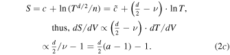
These inequalities are shown in Figure 1. (Here d denotes the spatial dimension and must not be confused with the effective dimensionality  , e.g., Livadiotis 2015a. The entropic dependence on T and n is taken from the Sackur–Tetrode entropic formula, e.g., Livadiotis & McComas 2013a; Livadiotis 2014.)

Figure 1. Polytropic spectrum: arrangement of thermodynamic processes along the interval of the (constant) polytropic index a or  Starting from
  (isochoric) and moving with increasing a (left to right), we find the four intervals of "Explosion," "Mild Explosion," "Sub-adiabatic," and "Super-adiabatic," which are characterized by 0, 1, 2, and 3 negative terms (noted in blue) out of the three {dS/dV, dT/dV, dP/dV}. The entropy S depends on the spatial dimension, which is taken to be d = 3. The adiabatic process corresponds to a = 1 + 2/d, thus a = 5/3 for d = 3.
Download figure:
Standard image High-resolution imageIn the last two decades the polytropic index of the solar wind has been estimated by analyzing various data sets of solar wind protons (e.g., Totten et al. 1995; Newbury et al. 1997; Kartalev et al. 2006; Nicolaou et al. 2014). Earlier, Winterhalter et al. (1984) estimated the polytropic index at the terrestrial bow shock by applying the MHD Rankine–Hugoniot conditions upstream and downstream of the shock. They estimated a polytropic index between 1.6 and 1.7, which is consistent with the adiabatic 5/3, while Zhuang & Russell (1981) found that a polytropic index a ≈ 2 fits the terrestrial bow shock better. As shown in Table 1, solar wind and planetary bow shocks are characterized by polytropic indices close to their adiabatic value. In fact, numerous analyses of space plasmas were performed using the adiabatic polytropic index, a = 5/3 (e.g., Zank 1999).
Table 1. Studies to Determine the Polytropic Index of the Solar Wind
| Study Reference | Resulting a | Data sets | Space Plasma |
|---|---|---|---|
| (1) Zhuang & Russell (1981) | 2 | ISEE-1 | Bow shock |
| (2) Tatrallyay et al. (1984) | 1.85 | Pioneer Venus Orbiter | Venus bow shock |
| (3) Winterhalter et al. (1984) | 1.6–1.7 | ISEE-1 | Bow shock |
| (4) Baumjohann & Paschmann (1989) | 1.67 ± 0.5, 1.4 | AMPTE/IRM | Plasma sheet |
| (5) Newbury et al. (1997) | 5/3, 2 | Pioneer Venus Orbiter | Solar wind |
| (6) Kartalev et al. (2006) | 0.5–2.5 | Wind | Solar wind |
| (7) Nicolaou et al. (2014) | 1.8 ± 2.4 | OMNI | Solar wind |
| (8) Totten et al. (1995) | 1.46, 1.58 | Helios-1 | Solar wind |
| (9) Osherovich et al. (1993) | 0.5, 0.6 | IMP-8 | Magnetic clouds |
| (10) Hammond et al. (1996) | 0.73, 0.78 | Ulysses/CMEs | CMEs |
| (11) Sckopke et al. (1981) | ∼0 | ISEE-1 and ISEE-2 | Magnetosheath |
| (12) Livadiotis et al. (2011) | −0.04 ± 0.07 | IBEX | Inner heliosheath |
| (13) Pang et al. (2015a) | −0.15, 0−1 | Cluster | Plasma sheet |
| (14) Nicolaou et al. (2015) | ∼0 | New Horizons | Jovian magnetosheath |
Note. The first two cases (1, 2) have polytropic indices 5/3 < a, noted in the region of "Super-adiabatic" processes. Cases (3–7) have polytropic indices close to a ∼ 5/3, noted as quasi-adiabatic processes. Case (8) refers to 1 < a < 5/3, noted as a "Sub-adiabatic" process. Studies of magnetic clouds (9) and CMEs (10) found polytropic indices 0 < a < 1, noted in the region of "Mild Explosion." The last four cases (11–14) indicate isobaric processes. (In case (12), see also Livadiotis & McComas 2012, 2013b; in case (13), see also Pang et al. 2015b. Note that the word "Terrestrial" has been ignored for those space plasmas for simplicity.)
Download table as: ASCIITypeset image
On the other hand, using the method of correlation maximization with the data derived from Livadiotis et al. (2011), Livadiotis & McComas (2013b) found that the polytropic index in the inner heliosheath is near zero (see also Livadiotis & McComas 2012; and Section 4 of the present paper). These anticorrelations of n–T, consistent with constant or quasi-constant thermal pressure P, were also found in the low-latitude boundary layer at the terrestrial magnetosheath (Sckopke et al. 1981), in the terrestrial central plasma sheet (Pang et al. 2015a, 2015b), and in the Jovian magnetosheath (Nicolaou et al. 2015). It is still unknown why thermodynamic processes in these space plasmas are isobaric (Figure 1).
Polytropic processes may vary along a flow streamline; thus, the polytropic index along a streamline may not have a fixed value. One example is the plasma flow near a shock. There are cases where the polytropic index of the plasma may have different values upstream and downstream of a shock (e.g., for the heliospheric termination shock, see Parker 1961; Nicolaou & Livadiotis 2016; or for any shock, see Livadiotis 2015a). Another example is when the polytropic index is quasi-constant along the same plasma streamline, i.e., varying randomly around some mean value following a Gaussian or some distribution (e.g., see Nicolaou et al. 2014). Slattery (1977) developed a generalized polytropic equation of state, called a "perturbed" polytropic equation of state, to describe the thermodynamic process of the matter inside the giant planets. According to this, the logarithm of pressure has an extra term that perturbs its polytropic behavior, that is, a polynomial expansion in powers of density (see also Horedt 2004). Finally, the superposition of polytropic indices is a topic that has not yet been investigated, either in theory or in applications.
The purpose of this paper is to study the generalized thermodynamic processes expressed as a random superposition of Gaussian polytropes. This involves the following:
- 1.Developing the theory, namely, the equation of state and Bernoulli's integral (the condition of energy conservation), first for a single polytrope and then for a superposition of polytropes with an arbitrary distribution of polytropic indices. Emphasis is placed on a Gaussian superposition of polytropes with all the derivations given analytically.
- 2.Applying the model of the Gaussian superposition of polytropes in the inner heliosheath. We find that the mean polytropic index is near zero, indicating an isobaric thermodynamic process and a concave-downward parabolic relation between the density and temperature (on a log–log scale). Then, the magnetic field in the inner heliosheath is estimated by applying Bernoulli's integral along the equator of the inner heliosheath. These estimated values are very similar to those derived from a different method, the large-scale quantization (Livadiotis 2015b). Finally, the values of density, temperature, polytropic index, and magnetic field help to determine the large-scale quantization constant to better precision.
The paper presents the analytical derivations of the equation of state and Bernoulli's integral in the case of a superposition of polytropes with application in the proton plasma of the inner heliosheath. First, Section 2 expounds the theory in the case of a fixed value of a polytropic index. The concept of invariant pressure under a polytropic thermodynamic process is explained. Next, in Section 3, the theory is extended for a superposition of polytropic indices. The superposition is characterized by some distribution of polytropic indices; here we consider a Gaussian distribution of polytropic indices around a mean value with some standard deviation. The equation of state and Bernoulli's integral are derived in detail. Section 4 shows the application of the Gaussian superposition of polytropes in the inner heliosheath. Section 5 describes the estimation of the magnetic field in the inner heliosheath by applying Bernoulli's integral along the equator of the inner heliosheath. A previous analysis, which was based on the concept of a large-scale quantization constant, had also revealed the magnetic field of the inner heliosheath. The findings of these two different approaches are surprisingly similar. Therefore, in Section 6, the findings are reversed, in order to derive the large-scale quantization constant to higher precision, using the magnetic field estimated by the present analysis. Finally, Section 7 summarizes the conclusions.
2. SINGLE POLYTROPE: EQUATION OF STATE AND BERNOULLI'S INTEGRAL
Consider a system of N particles with number density n, mass density  (particle mass m, total mass
  ), temperature T, and thermal pressure
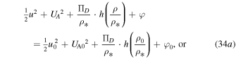
  that flows with bulk velocity u in a potential φ and magnetic field B. Then Bernoulli's integral for an incompressible fluid is
(μ is the permeability of the medium). Note that Bernoulli's integral is a condition of energy conservation (the one included in the Rankine–Hugoniot conditions, see Rankine 1870; Hugoniot 1887, 1889).
For two different points in the plasma flow streamline  and
and  , (3) gives
For a compressible fluid, the variation of the thermal term,  , is substituted by the integral
  .
.
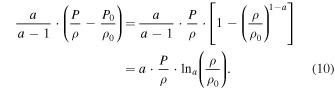
The generalized pressure,  , constitutes the invariant physical quantity that remains constant under a polytropic procedure; it is called the generalized polytropic invariant pressure, and it is defined by

where  is some characteristic density scale. The exponent a denotes the polytropic index (see Figure 1, Equations (2a)–(2c); and Livadiotis & McComas 2012). Assuming such a polytropic law, between the two different streamline points,

we obtain ![${\int }_{{\rho }_{0}}^{\rho }dP/\rho =[a/(a-1)]{P}_{0}{\rho }_{0}^{-a}({\rho }^{a-1}-{\rho }_{0}^{a-1})$](https://content.cld.iop.org/journals/0067-0049/223/1/13/revision1/apjs522835ieqn25.gif)
$](https://content.cld.iop.org/journals/0067-0049/223/1/13/revision1/apjs522835ieqn26.gif) . Hence, (4) becomes
. Hence, (4) becomes
The non-potential energy in the above equation can be written exclusively in terms of velocities:

where  is the Alfvén speed and
  is the characteristic thermal speed. Note that for a = 2 these two velocities can be summed like two different velocity components. This has been remarked by Zank et al. (2010), emphasizing that MHD Rankine–Hugoniot conditions are structurally identical to the usual hydrodynamic jump conditions with the isotropic magnetic field pressure contributing to the total pressure. Indeed, setting
  , the Rankine–Hugoniot conditions for the conservation of momentum and energy respectively become
 ![${\left[n\left({u}^{2}+\frac{1}{2}{U}^{2}\right)\right]}_{1}=$](https://content.cld.iop.org/journals/0067-0049/223/1/13/revision1/apjs522835ieqn30.gif)
![$\;{\left[n({u}^{2}+\frac{1}{2}{U}^{2})\right]}_{2}$](https://content.cld.iop.org/journals/0067-0049/223/1/13/revision1/apjs522835ieqn31.gif) and
and ![${\left[\frac{1}{2}{u}^{2}+{U}^{2}\right]}_{1}$](https://content.cld.iop.org/journals/0067-0049/223/1/13/revision1/apjs522835ieqn32.gif)
![$=\;{\left[\frac{1}{2}{u}^{2}+{U}^{2}\right]}_{2}$](https://content.cld.iop.org/journals/0067-0049/223/1/13/revision1/apjs522835ieqn33.gif) .
.
For adiabatic processes the thermal term becomes ![$[\gamma /(\gamma -1)]\cdot P/\rho $](https://content.cld.iop.org/journals/0067-0049/223/1/13/revision1/apjs522835ieqn34.gif) and coincides with the specific enthalpy. Indeed, the enthalpy of the system of N particles with f degrees of freedom each is
and coincides with the specific enthalpy. Indeed, the enthalpy of the system of N particles with f degrees of freedom each is 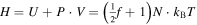 , where
  is the internal energy and
  is the product of pressure P and volume V of the system. The specific enthalpy is
  (where
  ), thus
  . In terms of the adiabatic index
  (where CP and CV are the heat capacities at constant pressure and constant volume, respectively), the specific enthalpy becomes
 ![${h}_{1}=[\gamma /(\gamma -1)]\cdot P/\rho $](https://content.cld.iop.org/journals/0067-0049/223/1/13/revision1/apjs522835ieqn42.gif) (where we substituted the ratio
(where we substituted the ratio  ). Hence, the integral (7b) becomes (Siscoe 1983)

Care must be shown for non-adiabatic processes,  , since the integral may be mistakenly thought to be given in terms of the enthalpy, which is true only for adiabatic
  (Kartalev et al. 2006).
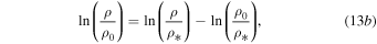
For isothermal processes a = 1, or even quasi-isothermal processes with  , Bernoulli's integral cannot be used as given in Equations (7a)–(7c), because the thermal term
 ![$[a/(a-1)]\;P/\rho $](https://content.cld.iop.org/journals/0067-0049/223/1/13/revision1/apjs522835ieqn47.gif) becomes infinite. As a solution to that problem, it could be mistakenly thought that for these processes the thermal term
becomes infinite. As a solution to that problem, it could be mistakenly thought that for these processes the thermal term ![$[a/(a-1)]\;P/\rho $](https://content.cld.iop.org/journals/0067-0049/223/1/13/revision1/apjs522835ieqn48.gif) takes a large value but remains constant at the same streamline, so it could be absorbed in the integral constant, i.e.,
takes a large value but remains constant at the same streamline, so it could be absorbed in the integral constant, i.e.,  ∼ constant. First, the thermal term is involved in Bernoulli's integral through the variation
 $](https://content.cld.iop.org/journals/0067-0049/223/1/13/revision1/apjs522835ieqn50.gif) (see Equation (7a)). This is proportional to
(see Equation (7a)). This is proportional to  , which does not grow to infinity for a → 1 because it turns to be indefinite (0/0). Second, it is well known that the thermal term is modified to
  . This can be easily shown as follows (e.g., Çengel et al. 2012):
  , so that Equation (7a) becomes


However, can Equations (7a)–(7c) be reduced to Equations (9a)–(9c) for a = 1? The answer is yes; this can be shown using the variation of the thermal term $](https://content.cld.iop.org/journals/0067-0049/223/1/13/revision1/apjs522835ieqn54.gif) and the polytropic law (6),
and the polytropic law (6),
The function  is the q-deformed natural logarithm (e.g., Silva et al. 1998; Yamano 2002; Livadiotis & McComas 2009; Livadiotis 2016), and its inverse function is the q-deformed exponential,
  . These are defined by
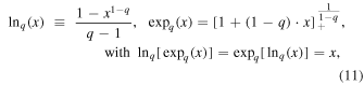
where the subscript "+" denotes the cut-off condition: ![${[x]}_{+}=x$](https://content.cld.iop.org/journals/0067-0049/223/1/13/revision1/apjs522835ieqn57.gif) if
if  and
and ![${[x]}_{+}=0$](https://content.cld.iop.org/journals/0067-0049/223/1/13/revision1/apjs522835ieqn59.gif) if
if  . The q-deformed logarithm and exponential functions recover to the ordinary logarithm
  and exponential
  for q → 1. Therefore, Equation (9a) becomes
(where  ). It can be easily shown that for any value of density
  , we have
which generalizes the respective identity of ordinary logarithms for a = 1,
Then, using the polytropic law (6), we obtain
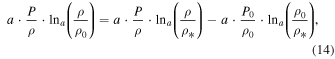
and thus Equation (14) is written as
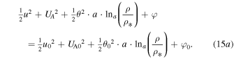
Finally, we end up with the formulation
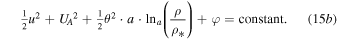
Both Equations (15a) and (15b) describe Bernoulli's integral for any value of a, where the scale  is arbitrary and not characteristic of the system (because of Equations (13a) and (13b)), and may represent the density units or be fixed to unity. Namely, the integral (15b) is reduced to Equation (9c) for a = 1 and to Equation (7c) for
  .
.
3. SUPERPOSITION OF POLYTROPES
3.1. The Multi-polytropic Equation of State
A possible generalization of Bernoulli's integral comes from a synthetic thermodynamic process that can be expressed as a superposition of polytropic processes. Given a density of polytropic indices, D(a), the generalized polytropic pressure,  , describes the physical quantity that remains invariant under thermodynamic processes of the pressure–density relation that generalizes Equation (5), that is
Then, Bernoulli's thermal term becomes
(where we set  ). As an example of D(a), we consider a Gaussian distribution of polytropic indices about the most frequent polytropic index a0, that is
Then, according to Equation (16), the generalized polytropic invariant pressure along the flow becomes
Therefore, the invariant pressure along the flow is given by
and it remains constant along streamlines of constant  . When
  , Equation (19a) recovers the case of single polytrope for
  , i.e.,
We may write the invariant pressure in terms of the arithmetic density n:

Substituting  and
and  , we obtain
(Based on the scales of mass density  and pressure
  , we have introduced the scales of (arithmetic) density
  and temperature
  .) Hence, the density–temperature relation is given by
In terms of the decimal logarithm,
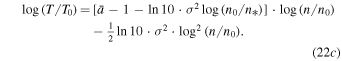
Hence,

with  ,
,  , and
, and  . This is a parabolic relation between the temperature and the density on logarithmic scales. Note that the density scale
  is not arbitrary, but all three parameters
  are characteristic of the proton population.
Therefore, the multi-polytropic equation of state is given by

or, in terms of the thermal pressure  and the invariant pressure
  ,
,

3.2. The Multi-polytropic Bernoulli's Integral
We rewrite Equation (24) in terms of mass density ρ,

and since  is constant along the streamlines,
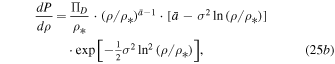
thus Bernoulli's thermal term Δ becomes
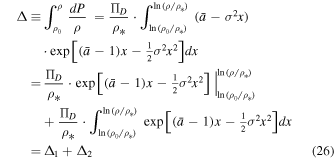
where we set  . Then,
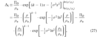
hence,
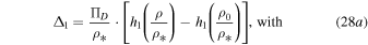

where we now set x ≡ ρ/ρ*; C1 is an arbitrary constant. Also,
hence,
where C2 is also an arbitrary constant. Both C1 and C2 may depend on  and σ.
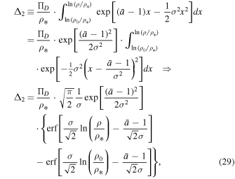
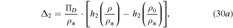
The term  becomes
Again, the function  is indefinite with respect to a constant,
  . A convenient choice is
i.e.,
Figure 2 shows Bernoulli's thermal term  as a function of the density ratio
  . We observe that as σ increases, the function
  becomes constant at high and low values of the density, while a local maximum appears at moderate densities near the characteristic density scale
  . Hence, the thermal term Δ has more effect on Bernoulli's integral for moderate densities near
  , while it may be ignored for more extreme densities. As σ decreases, the function
  approaches the standard case of a single polytropic index, where
  is given by a q-deformed logarithm for
  , according to Equation (11), which recovers the regular logarithm for
  = 1,
= 1,
Figure 2. Bernoulli's thermal term  is plotted against the density ratio
  . The plot is shown for various values of the mean polytropic index, (a)
  = 2, (b)
  = 1, (c)
  = 0.2, and of the standard deviation: σ = 2 (solid red), σ = 1 (dotted blue), σ = 0.7 (dashed green), σ = 15 (dash–dotted purple), σ = 0 (thin orange). We observe that as σ increases, a local maximum appears at densities near the characteristic scale
  , while the function becomes constant at higher and lower densities.
Download figure:
Standard image High-resolution imageThe approximations of the function  for small values of σ, or for small values of
  , are given by
where  ,
,  , and
, and  ,
,  (for n > 1).
The whole Bernoulli's integral becomes
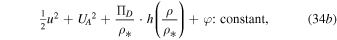
or, given Equation (25a),
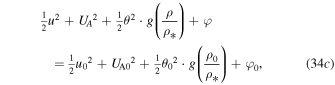
where

Finally, Figure 3 summarizes the analytical formulation of the function  that describes the thermal term in Bernoulli's integral.

Figure 3. Bernoulli's thermal term given by the function  for a Gaussian superposition (multi-polytrope) with non-isothermal
  or isothermal
  mean polytropic index, and its reduction to the single polytrope when
  .
.
Download figure:
Standard image High-resolution image4. GAUSSIAN SUPERPOSITION OF POLYTROPES IN THE INNER HELIOSHEATH
The Interstellar Boundary Explorer (IBEX) mission was launched in 2008 October to observe energetic neutral atom (ENA) emissions from the edge of the solar system where the subsonic solar wind interacts with the interstellar neutrals (McComas et al. 2009). IBEX images the sky via two ultrasensitive ENA detectors (IBEX-Hi, IBEX-Lo) and constructs  all-sky maps every ∼6 months, covering a broad energy range from ∼0.01 to ∼6 keV. Using ENA observations from the IBEX-Hi sensor with energies above ∼0.7 keV, Livadiotis et al. (2011) derived the sky maps of the (radially) average values of temperature, density, and other thermodynamic quantities of the ENA-source proton population in the inner heliosheath. This was developed by connecting the observed ENA flux to the kappa distribution of velocities of the source protons (see also Livadiotis et al. 2012, 2013).
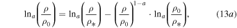
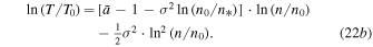
Livadiotis & McComas (2012, 2013b) showed the negative correlation between the values of temperature T and density n of the proton plasma along the equatorial streamline from the heliospheric nose toward the heliotail. More precisely, it was shown that the variations of T and n follow an isobaric polytropic index, i.e.,  (or
(or  ). Here, we show that the parabolic model (22d) is a better fit on the log–log scale of the observed values of T and n. The average polytropic index is still isobaric,
  , while we also derive the values of the polytropic standard deviation σ and the characteristic density scale
  . Since
  , the third coefficient in Equation (22d) is
  , thus the parabolic relation of
  is concave-downward. In addition, there is a characteristic density scale that separates the ENA-source plasma that is located near the equator from the ENA-source plasma that is located near the poles,
  (shown in Figure 9 of Livadiotis et al. 2011, and Figure 3 of Livadiotis & McComas 2012).
Next, we estimate the values of the triplet  for the proton plasma in the inner heliosheath. Figure 4 shows the fit of the parabolic relation Equation (22d) to the equatorial data of
  , from where we estimate the optimal values of the fitting parameters,
  ,
,  ,
,  . The value of σ is derived directly from
 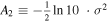 .
.
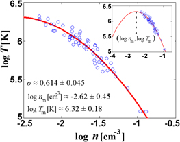
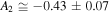
Figure 4. The parabolic fit between the density and temperature values (on a log–log scale) of the equatorial data of the inner heliosheath (derived from the analysis of Livadiotis et al. 2011). The square or curvature term, A2, is directly related to the standard deviation of polytropic indices, σ. The fit shows that there is a negative correlation between density and temperature values only for densities  (density units: cm−3); their correlation becomes positive for smaller densities.
Download figure:
Standard image High-resolution imageThe second term  can be used to derive the standard deviation, that is,
 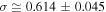 . The zeroth term,
  , is not useful as it does not directly depend on any of the triplet parameters
  . Both
  and
and  are included in
  , through the relation

The above linear relation is written as 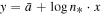 , where the values of the intercept
  and slope
  can be found from a second fitting, that of the linear relation between the known values of
  and
and  . Unfortunately, there is only one known pair of (x, y) as derived from the first fitting. We use the technique of the variation of the fitting parameters to produce more pairs of x and y.
This technique is useful when we want to investigate the correlation, if any, between the derived optimal values of the fitting parameters. Consider the case of fitting a model to M data points that leads to the optimal values of two modeling parameters, α and β. In order to examine the correlation between these parameters we need more than one pair of values. The technique of the variation of fitting parameters degenerates the pair of optimal values (α, β) into a whole set of N pairs, (α1, β1), ..., (αN, βN), so the relation between the parameters α and β can be examined. We describe the technique as follows.
If we remove one data point from the set of M data points, then we can derive the optimal parameter value from fitting the remaining (M − 1) data points. Thus, we may have M optimal parameter values, one for each of the combinations of removing m = 1 from M data points. Similarly, we can have  optimal values for all the combinations of removing m = 2 data points, and generally we can have
 ![${(}_{\;m}^{M})\equiv M!/[m!(M-m)!]$](https://content.cld.iop.org/journals/0067-0049/223/1/13/revision1/apjs522835ieqn146.gif) optimal values for all the combinations of removing m data points. Therefore, the number of all combinations of removing any number of data points less than or equal to m is
optimal values for all the combinations of removing m data points. Therefore, the number of all combinations of removing any number of data points less than or equal to m is  . Note that this number N is sufficiently large even when removing only a few data points, i.e., for M = 100 and m = 2 we have
  , and for m = 3 we have
  .
.
The estimated parameter values αi and βi (i = 1, ..., N ) are close to the initially estimated ones, α and β, and normally distributed about their averages  and
and  . Thus, the technique does not add information to the optimal values of the fitting parameters, but to the relation between the fitting parameters. (For an application of this technique, see Livadiotis et al. 2011, 2013.)
The above technique of the variation of the fitting parameters is applied to the  data shown in Figure 4. We produce 59 pairs of (xi, yi) values, where
  and
and  . Then their linearity is examined. A linear statistical model is fitted and, according to Equation (35),
  , the intercept is the mean polytropic index and the slope is the logarithm of the density scale.
Figure 5 shows the linear fitting, where we find  and
and 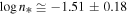 or
or 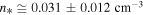 . (Compare with the value
 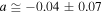 calculated with the method of maximized correlation in Livadiotis & McComas 2013b.) Then, substituting
  in Equation (22d), we find
 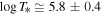 or
or  , while the invariant pressure is
  . Table 2 summarizes the results.
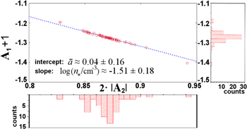
Figure 5. Application of the technique of the variation of the fitting parameters to determine the mean polytropic index  and the density scale
  . Using this technique we produce 59 pairs of the coefficients (
 ,
,  ,
,  ) of the parabolic fitting model used in Figure 4. Then we derive 59 pairs of (xi, yi) values, where
  and
and  . A second linear fitting on the (xi, yi) pairs determines the intercept, which is the mean polytropic index, and the slope, which is the logarithm of the density scale. Histograms of the x and y values are also shown.
Download figure:
Standard image High-resolution imageTable 2. Derived Parameters of the Gaussian Superposition of Polytropes in the Inner Heliosheath
| Thermodynamic Quantity | Estimated Value |
|---|---|
| Mean polytropic index |

|
| Polytropic standard deviation |

|
| Characteristic density scale |
|
| Characteristic temperature scale |
|
| Invariant pressure |

|
| Maximum temperature |
|
| Density at maximum temperature |

|
| Pressure at maximum temperature |
|
Download table as: ASCIITypeset image
Therefore, the inner heliosheath is likely characterized by Gaussian superposition of polytropes. The effective polytropic index,  , is given by
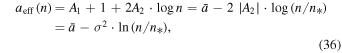
Figure 6 shows the three relations for the specific values of the triplet  , found for the proton plasma in the inner heliosheath (Table 2). The nonlinear relation between density and temperature leads to a density-dependent effective polytropic index. Therefore, different thermodynamic processes (e.g., adiabatic
  , isothermal
  , isobaric
  ; Livadiotis & McComas 2012) correspond to different densities.
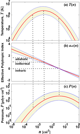
Figure 6. The effect of the polytropic superposition in the proton plasma of the inner heliosheath. (a) The temperature  , (b) the effective polytropic index
  , and (c) the thermal pressure
  are depicted as functions of density for the specific values of
  estimated for the inner heliosheath (red). Using the estimated errors
  , the 1σ deviations are also depicted (blue). Three special thermodynamic processes are indicated: adiabatic
  (for which
  is maximized), isothermal
  (for which
  is maximized), and isobaric
  (for which
  is maximized) (see also Figure 1).
Download figure:
Standard image High-resolution image5. ESTIMATION OF THE MAGNETIC FIELD IN THE INNER HELIOSHEATH
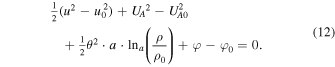
The constant of Bernoulli's integral can be found from its value at "infinity," i.e., in the direction of the hydrodynamic heliotail (downwind),
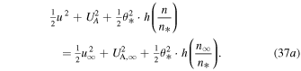
where the scale of the characteristic thermal speed,  , denotes the temperature
  in speed units. As was shown in Figure 2(c), the function h(x; a, σ) is negative for the values
  and
and  . Hence,
and substituting the Alfvén speed,
For u = 0 we derive the maximum possible magnetic field strength,
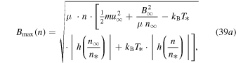
while for  we derive the minimum magnetic field,
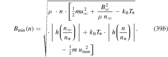
The speed  corresponds to the maximum possible, density-independent ion speed, for which the radicand in Equation (39b) is positive. Therefore, it depends on the rest of the parameter values, i.e.,
  . These extreme values, Bmin(n) and Bmax(n), determine the representative value of the average magnetic field,

The magnetic field is found to have values close to that given by Equations (38a) and (38b) for  , i.e.,
  . (This remark helps to estimate the uncertainty of
  , that is, the propagation error of all the parameters involved, including the uncertainty of the flow speed, which is taken as
  .) Figure 7(a) depicts the magnetic field of the inner heliosheath at the equator as a function of its plasma density, and for the values of
  ,
,  , a, and σ given in Table 2 and
  ,
,  , and
, and  given in Table 3. The magnetic field with the uncertainties, B(n) ± δB(n), is also shown. Once the magnetic field is determined, so are several other related plasma parameters. Figures 7(b) and (c) plot the Alfvén speed
  and the plasma beta parameter
 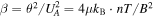 , respectively.

Figure 7. The estimated values of (a) the magnetic field, (b) the Alfvén speed, and (c) the plasma beta, for each value of density in the inner heliosheath. (These values are the radial averages along the heliocentric radius in the inner heliosheath, see Livadiotis et al. 2011.)
Download figure:
Standard image High-resolution imageTable 3. Parameters Involved in Bernoulli's Integral at "Infinity"
| Downwind Parameter | Value | Reference |
|---|---|---|
| Proton plasma density | 0.05 ± 0.03 cm−3 | Izmodenov (2009), Frisch et al. (2015), Zank et al. (2013) |
| Proton plasma speed | 26.3 ± 0.5 km s−1 | Möbius et al. (2004) |
| Magnetic field | 3 ± 0.5 μG | Izmodenov (2009), Heerikhuisen et al. (2014), Zank et al. (2013) |
Download table as: ASCIITypeset image
Having estimated the magnetic field strength as a function of the density in the inner heliosheath, it is now straightforward to construct the histogram of the values of the magnetic field that correspond to density data  (with N0 = 59) used in Figure 4 (derived from the analysis of Livadiotis et al. 2011). Applying Equation (39c) to
  , we derive the magnetic field strength values
  and their uncertainties
  . We avoid constructing directly the histogram of
  , because (i) the number of data N0 is not large enough to give a smooth and representative histogram and (ii) the uncertainties are also significant and thus must not be ignored. Therefore, we reproduce 1000 normally distributed data points, i.e.,
  for each of the original data points,
  . This technique produces
 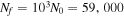 data points,
  .
.
Figure 8(a) shows the N0 data points of the estimated magnetic field,  . The Gaussian distribution
  is shown for the data point of largest density. Figure 8(b) shows the constructed normalized histogram of the magnetic field strength
  and its logarithm
  (inset). The mode of the histogram is located at B ≈ 1.7 μG. Interestingly, the logarithmic values of the magnetic field are normally distributed. Therefore, the representative average value of the magnetic field in the inner heliosheath is log B = 0.36 ± 0.03, or B = 2.29 ± 0.16 μG.

Figure 8. (a) Demonstration of the reproduction of 1000 normally distributed data points, i.e.,  for some original data point, B(n) ± δB(n). This technique produces Nf = 59,000 data points, that is, 1000 for each of the N0 = 59 original data points {Bi ± δBi}, i = 1, ..., N0, derived from Equation (39c). (b) Normalized histogram of all the Nf = 59,000 data points of the magnetic field B and its logarithm (inset). (c) Comparison with the normalized histogram of the magnetic field values of the inner heliosheath, which was derived from the usage of the large-scale-quantization constant in Livadiotis (2015b).
Download figure:
Standard image High-resolution imageThe normalized histogram of the magnetic field shown in Figure 8(b) is very similar to that constructed using a different method, the large-scale quantization. Livadiotis (2015b) derived the magnetic field values and their normalized histogram for the proton plasma in the inner heliosheath using (i) the density values of the whole sky (that is ∼1800 data points in contrast to the 59 equatorial data points) derived in Livadiotis et al. (2011), (ii) the value of the polytropic index a ≈ 0 found in Livadiotis & McComas (2013b), and (iii) the constancy of the fast magnetosonic energy over the plasma frequency (e.g., see Livadiotis & McComas 2014a). This histogram, with a mode also at B ≈ 1.7 μG, is shown in Figure 8(c). The matching of the two histograms in Figures 8(b) and (c) is intriguing for evaluation of the large-scale quantization theory, which is the topic of the next section.
6. LARGE-SCALE QUANTIZATION CONSTANT IN THE INNER HELIOSHEATH
Recent analyses of space plasmas revealed the existence of a new quantization constant ℏ*, similar to the Planck constant ℏ, but ∼12 orders of magnitude larger. Planck's constant constitutes the smallest possible phase-space parcel for individual and uncorrelated particles, while the new quantization constant describes the smallest possible phase-space parcel for collisionless particle systems characterized by local correlations (where correlations may be caused by Debye shielding, wave–particle long-range interactions, etc.). The majority of space plasmas throughout the heliosphere are such systems.
Local correlations are manifested by the presence of a correlation length between particles. This divides the system into an ensemble of clusters of correlated particles. The particles within each of these "correlation clusters" participate together in this new type of quantization. For example, the Debye length expresses a large-scale positional uncertainty among particles, thus assigning the smallest correlation length in plasmas (see Livadiotis & McComas 2014b). Thus, the standard quantization through the Planck constant  can occur to individual particles, and the large-scale quantization through the new constant
  applies only to clusters of correlated particles. The scheme in Figure 9 demonstrates how the large-scale quantization is related to the non-equilibrium statistics of space plasmas and the competition between correlations and collisions. The existence of correlations between particles shifts plasmas away from thermal equilibrium (Livadiotis 2015d) in stationary states described by kappa or kappa-like distributions (Livadiotis 2015c). These cannot embody the Boltzmann–Gibbs statistical mechanics, but rather the generalized framework of non-extensive statistical mechanics (Tsallis 2009). The stronger the correlation, the further the plasma resides from thermal equilibrium. On the other hand, collisions destroy correlations, returning plasmas to thermal equilibrium. Correlations, and thus the large-scale quantization, appear in collisionless plasmas, namely, in plasmas where the correlation length is smaller than the mean free path—the average collision length (Livadiotis 2014).
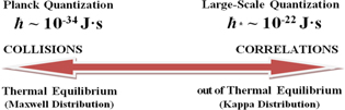
Figure 9. The non-equilibrium statistical behavior of space plasmas is related to the large-scale quantization constant. Both are caused by the presence of local correlations that survive in the collisionless plasma. (Taken from Livadiotis 2015b.)
Download figure:
Standard image High-resolution imageThe smallest energy E that can be transferred from a particle is related to the plasma frequency ω according to the well-known type of energy–frequency relation,  The amount of particle energy E that can be transferred away from the correlation cluster (e.g., the Debye sphere) sums the thermal and magnetic energies, leading to the magnetosonic energy
 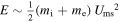 , where
  is the fast magnetosonic speed (mi, me are the ion/electron masses) (Livadiotis & McComas 2014a). Also, the frequency ω is typically given by the primary plasma frequency, ωpl. As a consequence, the value of
  can be approximated by
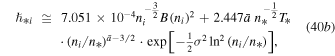
  , or
, or

where the units are  ,
,  ,
,  ,
,  also Te/Ti ≈ 1, and a is the mean polytropic index. Substituting Equation (23), and considering that a ∼
  , then we obtain
where the magnetic field  is taken from Equation (39c) (Section 5). Then, we derive a set of N0 = 59 values of
  (or
(or  ) with their uncertainties,
  .
.
Repeating the technique of Section 5, we reproduce 1000 normally distributed data points, i.e.,  for each original ith data point,
  hence, we end up with
  data points, namely,
  . Figure 10 shows the constructed normalized histogram of the derived values of the large-scale quantization constant,
  or
or  . The results reveal an accurate value of
  (Livadiotis & McComas 2013a, 2014b), i.e.,
 ![$\mathrm{log}{{\rm{\hslash }}}_{*}[{{\rm{J}}}_{{\rm{s}}}]=-21.84\pm 0.08$](https://content.cld.iop.org/journals/0067-0049/223/1/13/revision1/apjs522835ieqn250.gif) or
or  .
.

Figure 10. Using the magnetic field data {Bi ± δBi}, i = 1, ..., N0, derived from Equation (39c), as well as the respective density and temperature data, {ni, Ti}, we compute N0 = 59 values of the large-scale quantization constant,  , i = 1, ..., N0. Then, we multiply the number of data by 1000 using the technique explained in Figure 8(a), and finally we construct the normalized histogram of the Nf = 59,000 data points.
Download figure:
Standard image High-resolution imageIt must be noted that the objective of this section is not to show evidence for the existence of a large-scale quantization constant  . Whether the nature of
  is connected with a quantization or some other significant action/phase-space scale that characterizes plasmas is not important here. The important finding of this section is the value of this scale,
  , which is found to better precision. Evidence for quantization may be found elsewhere (Livadiotis & McComas 2013a, 2014a).
7. CONCLUSIONS
The paper has presented a possible generalization of Bernoulli's integral based on a synthetic thermodynamic process that can be expressed as a superposition of polytropic processes. First, the polytropic thermodynamic processes were shown for the case of a fixed value of a polytropic index. Then, the theory was extended for a superposition of polytropic indices. In general, the superposition may be described by any distribution of polytropic indices; here, a Gaussian distribution was considered, i.e., the polytropic indices were normally distributed around a mean value with some standard deviation. The theoretical development of the superposition of polytropic processes was the first objective of this paper, while next the theory was applied to the proton plasmas in the inner heliosheath.
In particular, we showed the following theoretical developments and applications in the inner heliosheath:
- 1.Development of the equation of state and Bernoulli's integral for a single polytrope and a superposition of polytropes, that is, a generalized polytropic thermodynamic process. In general, the superposition may be described by any distribution of polytropic indices. Emphasis was placed on the Gaussian superposition of polytropes, where all the generalized forms were derived analytically. The polytropic indices were normally distributed around a mean value with some standard deviation. The known linear density–temperature relation on a log–log scale now becomes a concave-downward parabola, where the parabolic curvature depends only on the standard deviation. The "invariant pressure" is the physical quantity that remains constant along the flow streamline of the generalized polytropic process. All the derived analytical forms, e.g., Bernoulli's integral (Equation (34b)), are expressed in terms of the invariant pressure.
- 2.Application of the model of the Gaussian superposition of polytropes to the proton plasma in the inner heliosheath, which led to a good fit of a concave-downward parabola relation to density and temperature data (on a log–log scale). The mean polytropic index is near zero (
 , ), indicating the dominance of isobaric thermodynamic processes (Table 2). Then, by computing Bernoulli's integral and applying its conservation along the equator of the inner heliosheath, the magnetic field in the inner heliosheath was estimated, B ≈ 2.29 ± 0.16 μG. Other relevant parameters were also estimated, e.g., Alfvén speed UA ≈ 102.5 km s−1 and plasma beta β ≈ 10 (Figure 7). Interestingly, the estimated magnetic field values are similar to those derived from a different method, the large-scale quantization (Livadiotis 2015b). Comparing the two methods helped to determine the large-scale quantization constant to better precision, namely, = −21.84 ± 0.08 or
.
, ), indicating the dominance of isobaric thermodynamic processes (Table 2). Then, by computing Bernoulli's integral and applying its conservation along the equator of the inner heliosheath, the magnetic field in the inner heliosheath was estimated, B ≈ 2.29 ± 0.16 μG. Other relevant parameters were also estimated, e.g., Alfvén speed UA ≈ 102.5 km s−1 and plasma beta β ≈ 10 (Figure 7). Interestingly, the estimated magnetic field values are similar to those derived from a different method, the large-scale quantization (Livadiotis 2015b). Comparing the two methods helped to determine the large-scale quantization constant to better precision, namely, = −21.84 ± 0.08 or
.


![$\mathrm{log}{{\rm{\hslash }}}_{*}[{\rm{J}}\;{\rm{s}}]$](https://content.cld.iop.org/journals/0067-0049/223/1/13/revision1/apjs522835ieqn258.gif)

The paper provides the complete theory of the superposition of polytropes for describing the flow along streamlines of space/astrophysical plasmas. The full strength and capability of this theory is thus available for the space physics/astrophysics community to study and to improve the modeling of polytropic thermodynamic processes. Moreover, the important findings of the application of the Gaussian superposition of polytropes in the inner heliosheath, e.g., the magnetic field estimations, will help in understanding the physics of the outer heliospheric boundary.